The VMC Survey

We derive the star formation history (SFH) for several regions of the Large Magellanic Cloud (LMC), using deep near-infrared data from the VISTA near-infrared $YJ\mbox{$K_{\rm s}$}$ survey of the Magellanic system (VMC). The regions include three almost-complete 1.4 deg² tiles located $\sim\!3.5^{\circ}$ away from the LMC centre in distinct directions. They are split into $21.0\arcmin\times 21.5\arcmin$ (0.12 deg²) subregions, and each of these is analysed independently. To this dataset, we add two $11.3\arcmin\times 11.3\arcmin$ (0.036 deg²) subregions selected based on their small and uniform extinction inside the 30 Doradus tile. The SFH is derived from the simultaneous reconstruction of two different colour–magnitude diagrams (CMDs), using the minimization code StarFISH together with a database of “partial models” representing the CMDs of LMC populations of various ages and metallicities, plus a partial model for the CMD of the Milky Way foreground. The distance modulus $(m\!-\!M)_{0}$ and extinction $A_{V}$ is varied within intervals $\sim\!0.2$ and $\sim\!0.5$ mag wide, respectively, within which we identify the best-fitting star formation rate ${\rm SFR}(t)$ as a function of lookback time $t$, age–metallicity relation (AMR), $(m\!-\!M)_{0}$ and $A_{V}$. Our results demonstrate that VMC data, due to the combination of depth and little sensitivity to differential reddening, allow the derivation of the space-resolved SFH of the LMC with unprecedented quality compared to previous wide-area surveys. In particular, the data clearly reveal the presence of peaks in the ${\rm SFR}(t)$ at ages $\mbox{$\log(t/{\rm yr})$}\simeq 9.3$ and $9.7$, which appear in most of the subregions. The most recent ${\rm SFR}(t)$ is found to vary greatly from subregion to subregion, with the general trend of being more intense in the innermost LMC, except for the tile next to the N11 complex. In the bar region, the ${\rm SFR}(t)$ seems remarkably constant over the time interval from $\mbox{$\log(t/{\rm yr})$}\simeq 8.4$ to $9.7$. The AMRs, instead, turn out to be remarkably similar across the LMC. Thanks to the accuracy in determining the distance modulus for every subregion – with typical errors of just $\sim\!0.03$ mag – we make a first attempt to derive a spatial model of the LMC disk. The fields studied so far are fit extremely well by a single disk of inclination $i=26.2\pm 2.0^{\circ}$, position angle of the line of nodes $\theta_{0}=129.1\pm 13.0^{\circ}$, and distance modulus of $\mbox{$(m\!-\!M)_{0}$}=18.470\pm 0.006$ mag (random errors only) up to the LMC centre. We show that once the $(m\!-\!M)_{0}$ values or each subregion are assumed to be identical to those derived from this best-fitting plane, systematic errors in the ${\rm SFR}(t)$ and AMR are reduced by a factor of about two.

1 Introduction

The VISTA near-infrared $YJ\mbox{$K_{\rm s}$}$ survey of the Magellanic system (VMC; Cioni et al. 2011) is performing deep near infrared imaging in the filters $Y$, $J$ and $K_{\rm s}$ for a wide area across the Magellanic system, using the VIRCAM camera (Dalton et al. 2006) on VISTA (Emerson et al. 2006). One of VMC’s main goals is the derivation of the complete spatially resolved star formation history (SFH) across the system. To this aim, the survey has been designed so that the photometry reaches magnitudes as deep as the oldest main sequence turn-off (MSTO), for both LMC and SMC, with signal-to-noise ratios of $\sim\!10$. Extensive pre-survey simulations of VMC images and its SFH-recovery by Kerber et al. (2009) indicated that this goal could be reached even in the most crowded areas of the LMC bar.

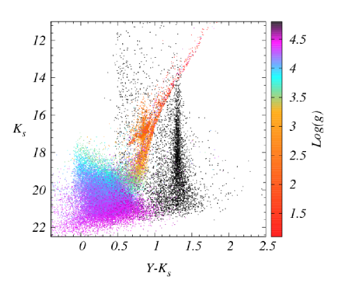
Figure 1: Simulated CMD for a 0.037 deg² region of moderate stellar density in the LMC. The black points show the distribution of the Milky Way foreground. The coloured dots show the LMC stars according to their surface gravity (in c.g.s. units).

Although the derivation of the SFH from photometry down to the old MSTO is now routinely performed for most galaxies in the Local Group (e.g., Orban et al. 2008; Noël et al. 2009; Williams et al. 2009; Hidalgo et al. 2011; Weisz et al. 2011, and references therein), this is effectively the first time that such a method has been tried using data from a near-infrared wide-area survey. The use of near-infrared filters has the obvious advantage that the CMDs are less affected by extinction and reddening (and their differential effects) than optical ones. On the other hand, they are much more affected by the presence of foreground Milky Way stars. Fig. 1 shows an example of a simulated colour–magnitude diagram (CMD) for the LMC field, derived as in Kerber et al. (2009) using the specifications of VMC, in which the different colours code the stellar gravities of the observed stars. The presence of two almost-vertical strips composed of Milky Way dwarfs is striking: there is a prominent one at $\mbox{$Y\!-\!K_{\rm s}$}\simeq 1.3$ mag, and a less defined one just redward of $\mbox{$Y\!-\!K_{\rm s}$}\simeq 0.5$ mag. These features partially overlap the red giant branch and helium burning sequences of LMC stars. Fortunately, they exhibit also a smooth and well understood behaviour as a function of Galactic coordinates, and do not affect in any way the interpretation of the stars on the LMC main sequence and turn-off.

First results from the VMC survey are described in Cioni et al. (2011), Miszalski et al. (2011a, b), and Gullieuszik et al. (2011). In this paper, we present the recovery of the SFH for part of the LMC using the first season of VMC data. The data and their preparation for this work are briefly described in Sect. 2. Sect. 3 presents the basic results regarding the star formation rate as a function of lookback time, ${\rm SFR}(t)$, and the age–metallicity relation, AMR. The minimization method employed allows us to estimate also the distance and extinction for each examined subregion. The geometry inferred for the LMC disk is discussed in Sect. 4. In Sect. 5 we adopt this revised geometry and revise the results for the ${\rm SFR}(t)$ and AMR, obtaining a significant reduction of the error bars. Finally, we draw some general conclusions, and compare our results with previous works.

2 The VMC data

The VMC survey and its initial data are thoroughly described in Cioni et al. (2011), to which we refer for all details. We have recovered the SFH from VISTA data for three VMC tiles located around the main body of the LMC and for which the VISTA imaging is most complete. Details about these tiles, and their sub areas, are presented in Table 1. Moreover we have used 2 small subregions in the more central 6_6 tile, which comprises 30 Doradus. The subregions were selected on the basis of the extinction maps derived by Tatton et al. (in prep.), as having a small and almost-constant extinction. Fig. 2 shows the location of all LMC tiles of the VMC survey (red rectangles). The black rectangles mark those used in this work.

Table 1: VMC tiles used in this work.

Tile name	$\alpha$ (J2000)	$\delta$ (J2000)	completion in $K_{\rm s}$-band	comments
4_3	04:55:19.5	$-$72:01:53	63%
6_6	05:37:40.0	$-$69:22:18	100%	30 Dor field
8_3	05:04:53.9	$-$66:15:29	75%
8_8	05:59:23.1	$-$66:20:28	90%	South Ecliptic Pole region

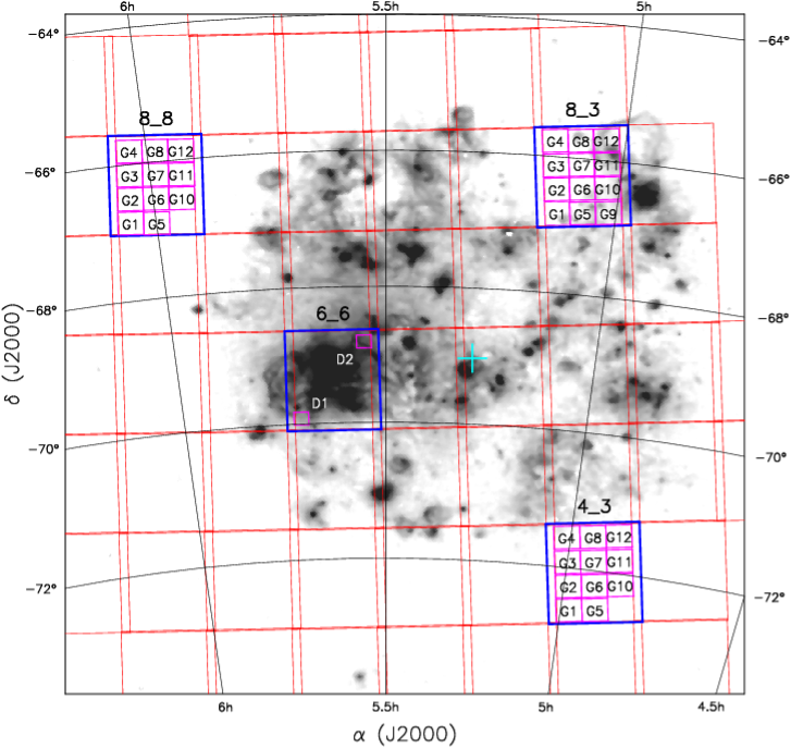
Figure 2: An H$\alpha$ image of the central LMC from the Southern H-Alpha Sky Survey Atlas (in gray; Gaustad et al. 2001), with VMC tiles marked by red rectangles. The blue and magenta rectangles show the positions of the tiles and subregions, respectively, considered in this work. The cyan cross marks the centre of the LMC as derived by Nikolaev et al. (2004).

We used the v1.0 VMC release pawprints. The pawprints were processed by the VISTA Data Flow System (VDFS, Emerson et al. 2004) in its pipeline (Irwin et al. 2004) and retrieved from the VISTA Science Archive (VSA, Hambly et al. 2004). We combined the calibrated pawprints into deep tiles with the SWARP tool (Bertin et al. 2002). The 4_3, 8_3, and 8_8 tiles, covering areas of $\sim 1.4$ deg² each, were subdivided into twelve subregions of $21.0\arcmin\times 21.5\arcmin$ ($\sim 0.12$ deg²), as illustrated in Fig. 2. In the 6_6 tile, the selected subregions are smaller ($11.3\arcmin\times 11.3\arcmin$ each, or $\sim 0.036$ deg²).

The pawprints contributing to corner subregion G9 (see Fig. 2) include a contribution from the “top” half of VIRCAM detector number 16 which is known to show a significantly worse signal-to-noise ratio than the other detectors because its pixel-to-pixel quantum efficiency seems to vary on short timescales making accurate flatfielding impossible. The effect is negligible in $K_{\rm s}$, small in $H$ and becomes more noticeable in the bluer bands, i.e. $J$, $Y$ and $Z$. Therefore subregions G9 of tiles 4_3 and 8_8 are not further considered. 8_3 is used as its signal-to-noise in G9, in the $Y$ band, was just $\sim 16$ % smaller than in neighbouring subregions.

2.1 Photometry and Artificial Star Tests

We performed point spread function (PSF) photometry using the IRAF DAOPHOT packages (Stetson 1987), generating photometric catalogues and CMDs. We used the PSF package to produce the PSF model (variable across the subregion), and the ALLSTAR package to perform the photometry using a radius of three pixels (2.5 pixels in the case of the 6_6 tile). We checked that our PSF photometry produced results consistent with those provided by VSA for the bulk of the observed stars. For the SFH-recovery work, PSF photometry was preferred to aperture photometry because it produced deeper catalogues, especially in the case of the highly crowded regions in the 6_6 tile.

Fig. 3 shows some examples of $K_{\rm s}$ vs. $Y\!-\!K_{\rm s}$ CMDs, for the subregion G3 of tiles 8_8, 8_3, and 4_3, and for the subregion D2 in the 6_6 tile.

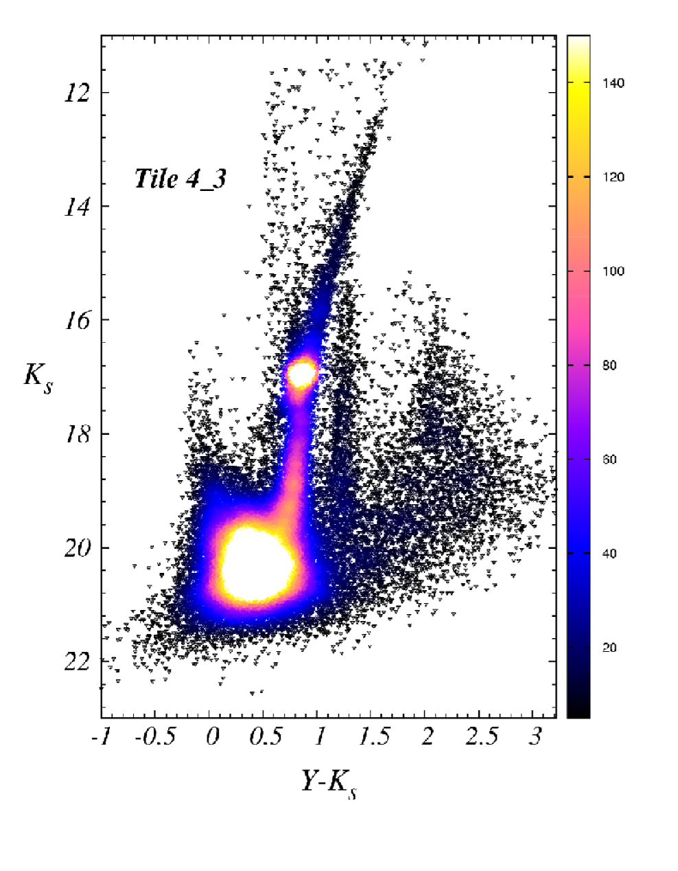
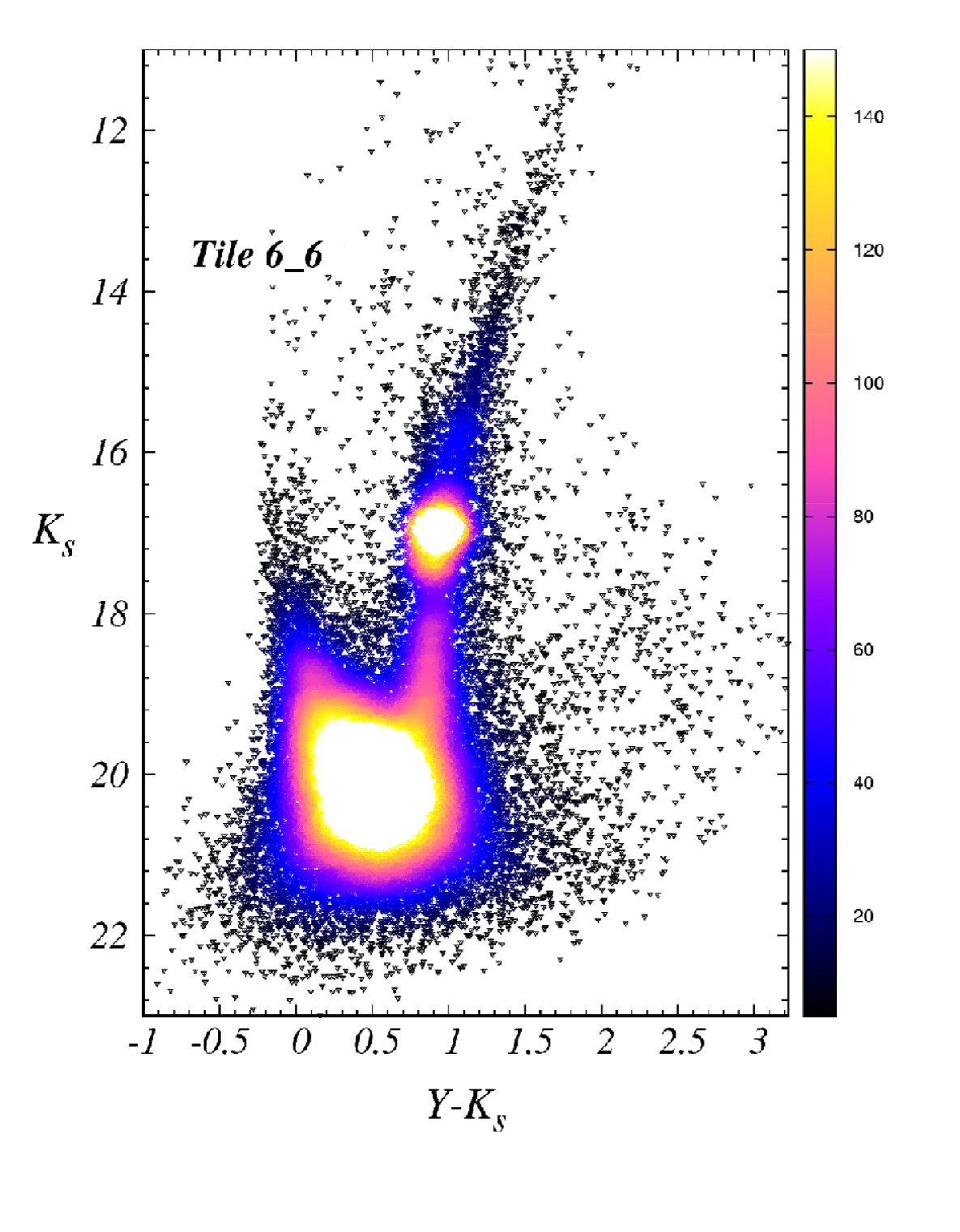
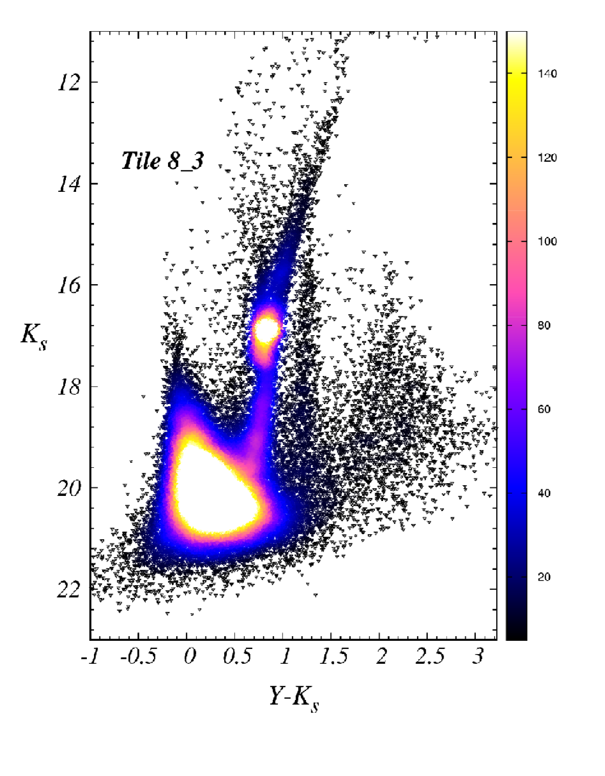
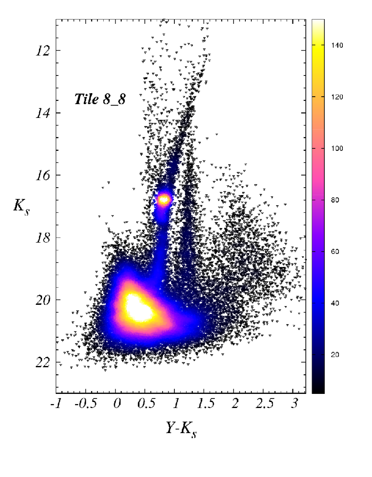
Figure 3: Examples of $K_{\rm s}$ vs. $Y\!-\!K_{\rm s}$ CMDs in subregions of the 4_3 (top left), 6_6 (top right), 8_3 (bottom left) and 8_8 (bottom right) tiles. An arbitrary color scale is used to highlight the CMD regions with a higher density of stars.

We have recovered the SFH using two CMDs simultaneously, namely $K_{\rm s}$ vs. $Y\!-\!K_{\rm s}$ and $K_{\rm s}$ vs. $J\!-\!K_{\rm s}$. We recall that the contamination by compact galaxies can be mostly prevented by simply eliminating objects with $\mbox{$J\!-\!K_{\rm s}$}>0.88$ mag and $\mbox{$Y\!-\!K_{\rm s}$}>1.56$ mag (see Kerber et al. 2009) from our data. This is done later in our analysis (see Sect. 3).

We have run large numbers of artificial star tests (ASTs) to estimate the incompleteness and error distribution of our data for each subregion and in every part of the CMD. For each subregion we ran $\sim\!2.8\times 10^{6}$ ASTs as described in Rubele et al. (2011), using a spatial grid with 30 pixels width and with a magnitude distribution proportional to the square of the magnitude. This latter choice allows us to better map completeness and errors in the less complete regions of the CMD.

Figure 4 shows an example, based on an 8_3 tile subregion, of the error distribution derived from ASTs in $Y$, $J$, and $K_{\rm s}$ versus the difference between the output and input magnitude. Fig. 5 shows an example, for a tile 8_8 subregion, of the completeness across the $K_{\rm s}$ vs. $J\!-\!K_{\rm s}$ CMD.

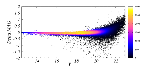
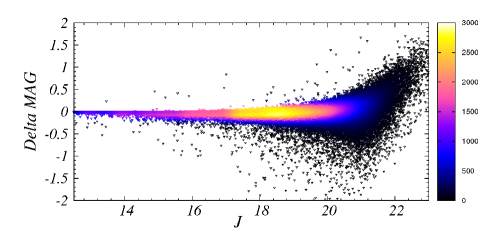
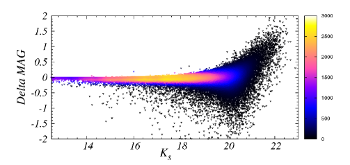
Figure 4: Examples of error distributions derived from the ASTs, in $Y$, $J$, $K_{\rm s}$ filters for a subregion of the 8_3 tile. An arbitrary color scale is used to highlight the regions with a higher density of stars.

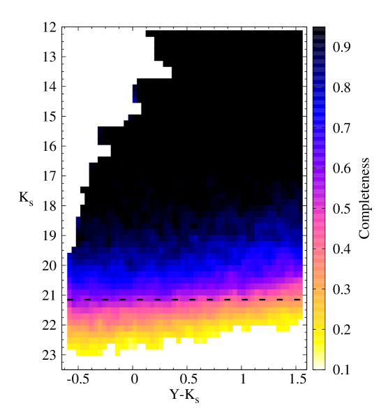
Figure 5: Example of completeness map derived from the ASTs on a $K_{\rm s}$ vs. $Y\!-\!K_{\rm s}$ CMD. The colours code the completeness level. The black dashed line shows the $5\sigma$ depth (or ${\rm S/N}=5$) in the $K_{\rm s}$ band.

2.2 Converting models and data to the same zeropoints

For the present work, we have converted large sets of theoretical stellar evolutionary models (see Marigo et al. 2008, and references therein) to the VISTA Vega magnitude system (Vegamag) which is itself derived from the 2MASS system, and where Vega has a magnitude equal to 0 in all filters. The procedure is thoroughly discussed in Girardi et al. (2002, 2008). The filter transmission curves employed are the official ones. The model isochrones, extinction coefficients, and other miscellaneous data, are retrievable via the web interface at http://stev.apd.inaf.it/cmd.

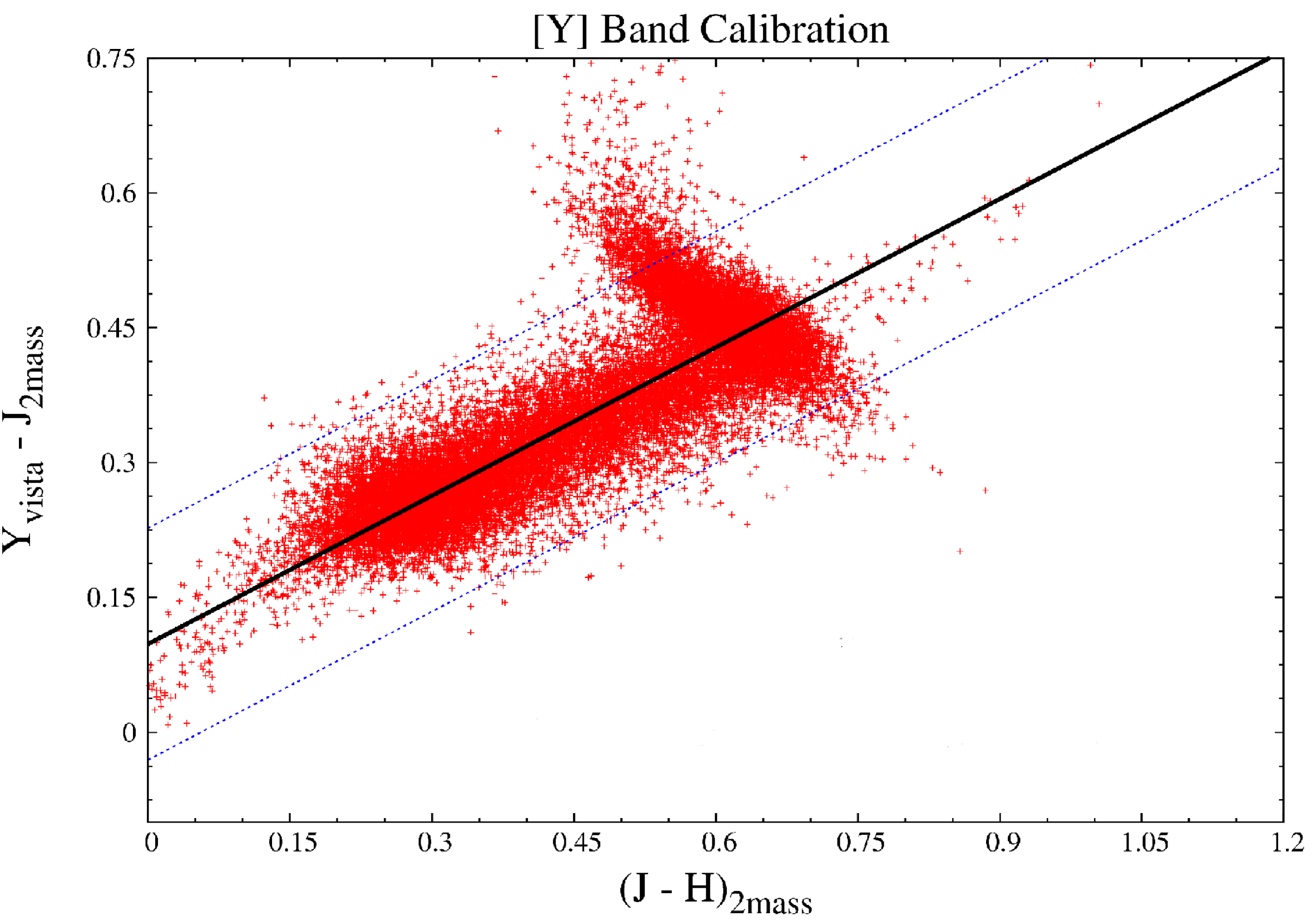
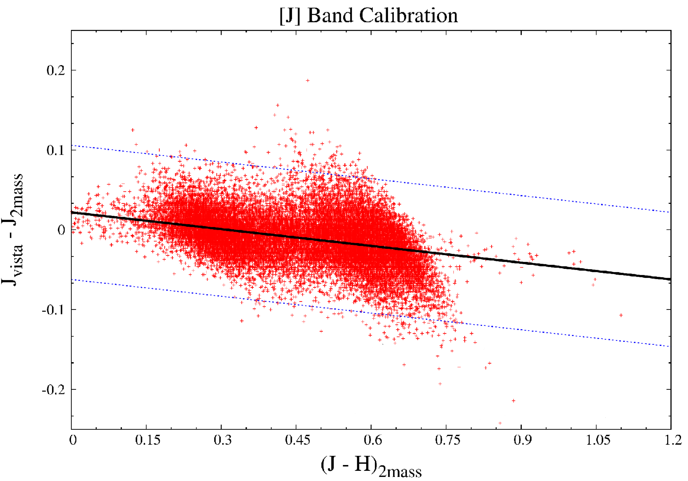
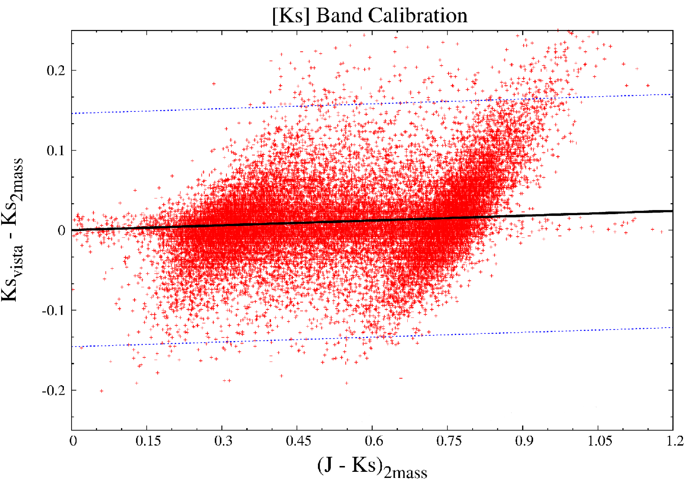
Figure 6: Calibration to the Vegamag system. The points show Milky Way model stars generated with the TRILEGAL model for an area of $\sim\!1.4$ deg², and convolved with the typical photometric errors of 2MASS. The dashed lines show the limits for the $3\sigma$ clipping. The continuous lines are the best-fitting linear relations with a fixed slope as in Eq. (1).

The photometric calibration of v1.0 VISTA pipeline processed pawprints by the pipeline processing group uses a similar approach to that for WFCAM data (Hodgkin et al. 2009) although the details of the colour equations are different for VISTA, and VISTA, like 2MASS, has a $K_{\rm s}$ filter whereas WFCAM has $K$.

The present zero point (ZP) calibration is based on using the 2MASS stars with $0<(\mbox{$J\!-\!K_{\rm s}$})_{\rm 2MASS}<1$ which fall on each detector in each pawprint to calculate their magnitudes on the VISTA system using the following linear fits for stars distributed all across the sky:

$$Y_{\rm VISTA}-J_{\rm 2MASS} = 0.550\,(J\!-H\!)_{\rm 2MASS}$$

$$J_{\rm VISTA}-J_{\rm 2MASS} = -0.070\,(J\!-\!H)_{\rm 2MASS}$$ (1)

$$\mbox{$K_{\rm s}$}_{\rm VISTA}-\mbox{$K_{\rm s}$}_{\rm 2MASS} = 0.020\,(J\!-\!K_{\rm s})_{\rm 2MASS}$$

with a small correction for mean extinction in the general area. The derived magnitudes of the 2MASS stars in the VISTA system are then used to calibrate each detector at each pointing by deriving the median ZP of each detector at that time. The $0<(\mbox{$J\!-\!K_{\rm s}$})_{\rm 2MASS}<1$ colour selection ensures that very blue and very red stars are not used in calibrating each tile.

The resulting VISTA magnitudes should then be on a Vegamag system assuming the colour relations used are accurate. However deviations from the true Vegamag zero points would result if these relations are not strictly linear, but have second-order terms, or inaccurate coefficients. Such second-order terms have been well characterized in WFCAM data by Hodgkin et al. (2009), but are not yet available for VIRCAM.

The current photometric calibration may thus not be precisely on the Vegamag system, especially in $Y$ where the greatest extrapolation from 2MASS $J$ is required. Therefore, before performing any detailed data–model comparison, we choose to convert the models to the same ZPs as the v1.0 data. This is done internally, without modifying the isochrones being distributed at http://stev.apd.inaf.it/cmd. Indeed, this procedure is the more convenient since future VISTA data releases may have different definitions of their ZPs.

To correct the observational ZPs we proceed as follows. We take the present stellar models and build the theoretical counterpart of the calibration data, using the TRILEGAL code (Girardi et al. 2005) to simulate field stars in the VISTA Vegamag system, and in 2MASS (using Maíz-Apellániz 2007 zeropoints). Photometric errors are added to the 2MASS data, following the error distributions inferred from Bonatto et al. (2004) in low-density regions of the sky. The derived simulations are shown in Fig. 6; they show colour ranges and distributions in the colour-colour plots which are very similar to those found in the real WFCAM data (see e.g. Hodgkin et al. 2009). Then, to the simulated data we fit a set of lines with the same slopes as in Eqs. (1). The outcome of the fitting is a set of constants, which are then interpreted as the ZP offsets between the VDFS pipeline v1.0 calibration and the Vegamag system of the stellar models. The offsets we find are equal to 0.099 mag in $Y$, 0.021 mag in $J$ and 0.001 mag in $K_{\rm s}$, with respect to the v1.0 calibration. These offsets are subtracted from our models before starting the SFH-recovery work.

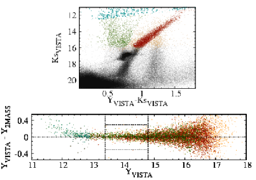
Figure 7: Verification of Eq. 1 when applied to real LMC data. The top panel shows stars in the 8_8 tile, in the $K_{\rm s}$ vs. $Y\!-\!K_{\rm s}$ diagram of VMC. Different colours are used for likely LMC giants (brown), likely Milky Way dwarfs (green), stars bright enough to be partially saturated (cyan), and stars for which 2MASS photometry is not available (black). The bottom panel shows the difference between the $Y$ magnitude as measured from VMC data, and as inferred from 2MASS photometry via the first Eq. (1), as a function of $Y$, for stars with both VISTA and 2MASS photometry. The vertical dashed lines denote the magnitude interval for which this comparison is the most significant, as discussed in the text.

The bulk of the stars shown in Fig. 6 are dwarfs in the solar vicinity. We check if applying this calibration method to the LMC result in any bias/offset in the calibration because of the nature of the stellar objects in the LMC tiles. To this aim we use the stars in the 8_8 tile for which we have both 2MASS and VISTA magnitudes, as ilustrated in Fig. 7. The top panel shows the $K_{\rm s}$ vs. $Y\!-\!K_{\rm s}$ diagram from VMC, which is used for a rough classification into likely Milky Way dwarfs and likely LMC giants. Then, we limit the sample to stars of intermediate brightness, so as to avoid including long-period variables and partly saturated objects in VMC at $\mbox{$K_{\rm s}$}<13.4$ mag, and stars with large photometric errors in 2MASS at $\mbox{$K_{\rm s}$}>14.8$ mag. The bottom panel plots the difference between the $Y$ magnitudes derived from VMC data and those derived from application of Eq. 1 to 2MASS photometry, as a function of $Y$. The $1\sigma$ dispersion at $13.4<\mbox{$K_{\rm s}$}<14.8$ is equal to $\simeq 0.065$ mag for both dwarfs and giants, and is likely dominated by the errors in 2MASS photometry. The offset between the two estimates of $Y$-band magnitude is just 0.005 mag for the likely LMC giants, and 0.019 mag for the likely Milky Way dwarfs. In both cases the offset is much smaller than the dispersion in the data, and less than the random errors we claim in the determination of the LMC distance moduli (see Sect. 4). Moreover, what is particularly reassuring in this comparison is that differences in the mean $Y$-band offsets between dwarfs and giants are just $\sim 0.01$ mag, despite the different color ranges comprised by both samples. We conclude that application of Eq. 1 in VMC field 8_8 does not appear to introduce any significant systematic error in the calibration.

3 The SFH recovery

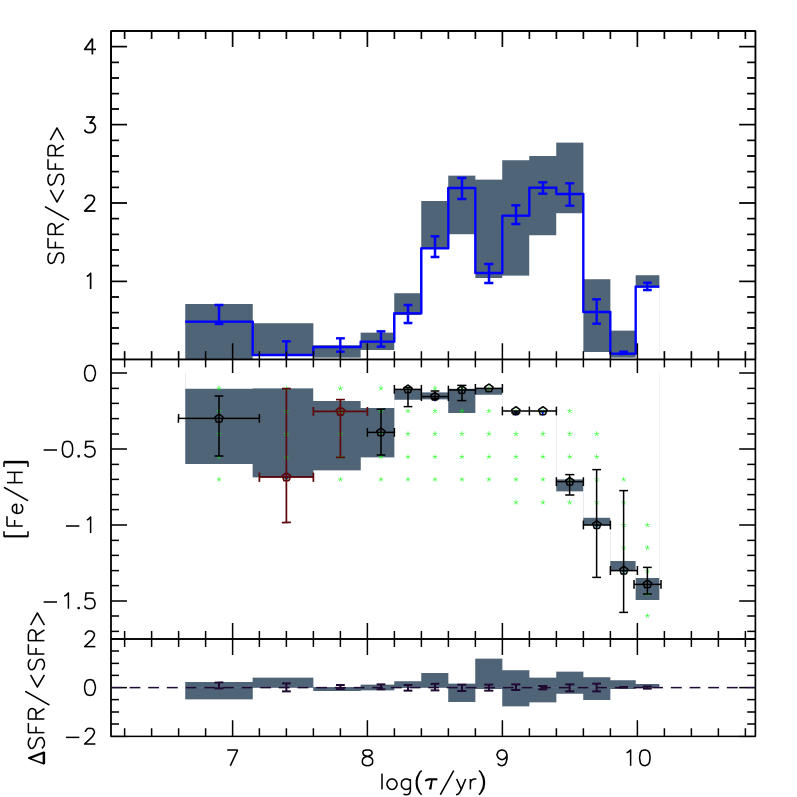
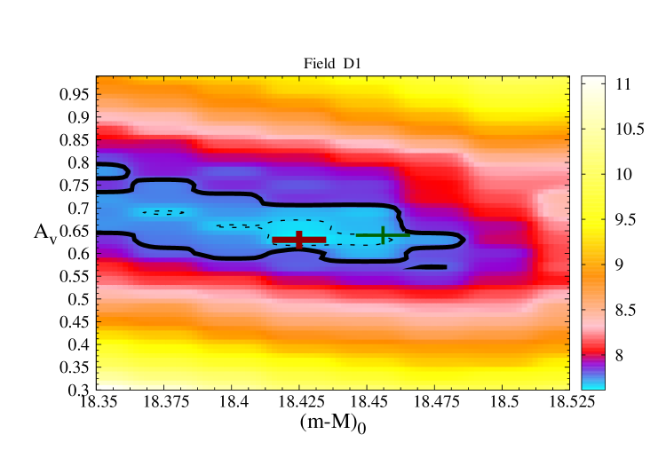
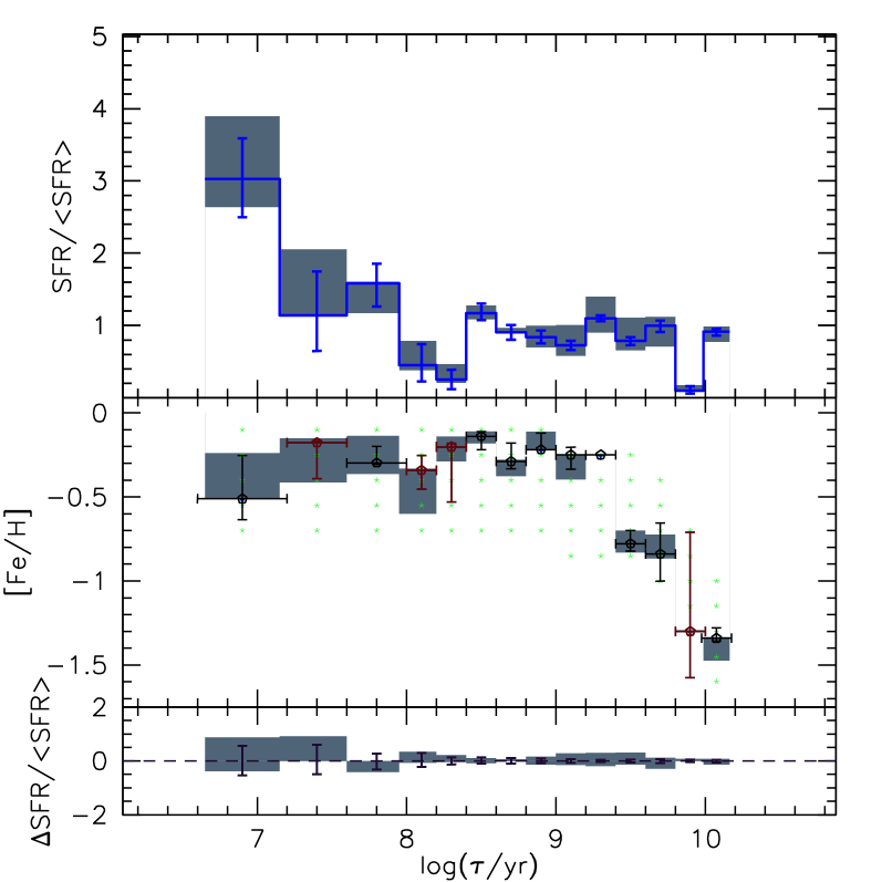
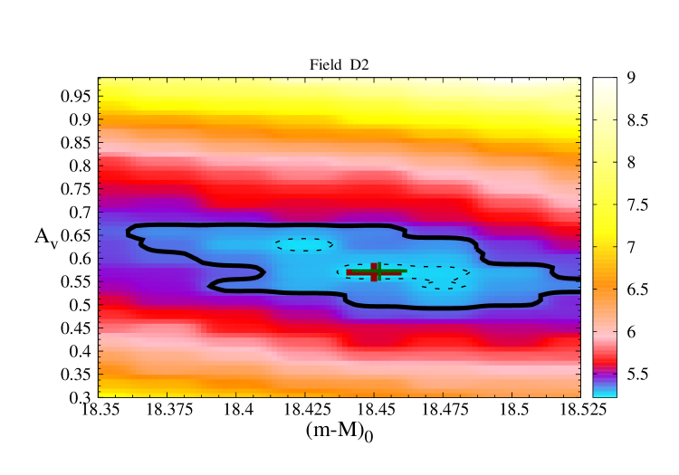
Figure 10: Same as Fig. 9 but for tile 6_6. Both subregions in this tile are presented.

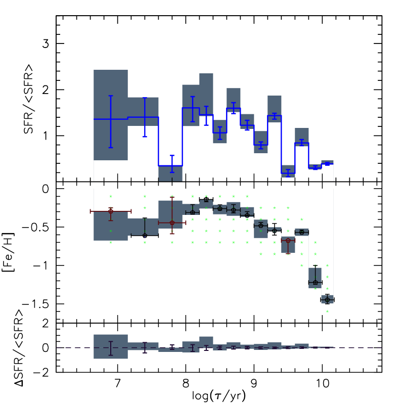
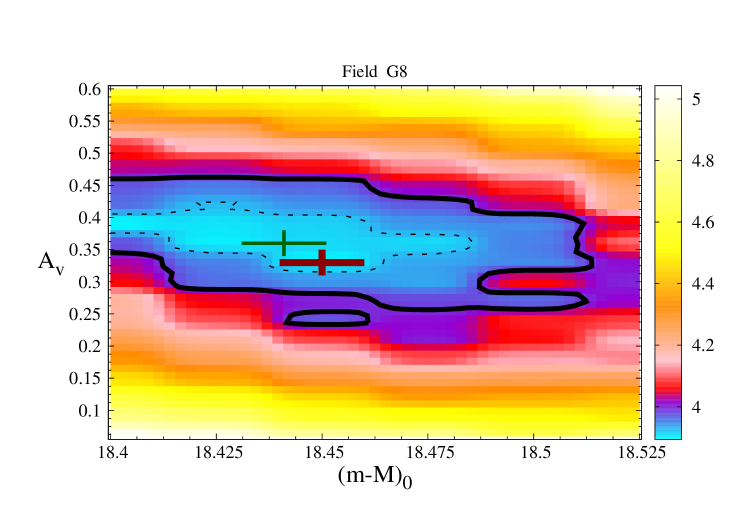
Figure 11: Same as Fig. 9 but for tile 8_3.

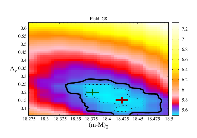
Figure 12: Same as Fig. 9 but for tile 8_8.

Our SFH-recovery work is largely based on Kerber et al. (2009), to which we refer for more details and basic tests of the algorithms. Here, we briefly mention the particular assumptions adopted in the present work. To recover the SFH we used a set of “stellar partial models” (SPMs), which are model representations of stellar populations covering small intervals of ages and metallicities, and observed at the same conditions of completeness and crowding as the real data. They are distributed over 14 age intervals that cover from $\log(t/{\rm yr})=6.6$ to $10.15$. They also follow five different AMRs located parallel on a [Fe/H] vs. age (or lookback time) plot. These AMRs cover those observed for stellar clusters (Olszewski et al. 1991; Mackey & Gilmore 2003; Grocholski et al. 2006; Kerber et al. 2007) and field stars (Harris & Zaritsky 2004, 2009; Cole et al. 2005; Carrera et al. 2008). Hence, LMC populations are described as linear combinations of 70 distinct SPMs. Table 2 shows their central values of $\log(t/{\rm yr})$ and [Fe/H]; they are also indicated as green starred points in Figs. 9–12. The width of each SPM is 0.15 dex in [Fe/H] and 0.2 dex in $\Delta\log(t)$, except for the 3 youngest age bins where we used $\Delta\log(t)$ widths of 0.6, 0.4 and 0.4 dex, respectively, and for the oldest age bin where we used 0.15 dex. Inside the age and [Fe/H] intervals of each SPM, the star formation rate is assumed to be constant.

The LMC populations are simulated using the Chabrier (2001) log-normal initial mass function, plus a 30 % binary fraction. The simulated binaries are non-interacting systems with primary/secondary mass ratios evenly distributed in the interval from 0.7 to 1.

Table 2: Grid of stellar partial models used in the SFH recovery.

$\log(t/{\rm yr})$	$\mbox{\rm[{\rm Fe}/{\rm H}]}_{1}$	$\mbox{\rm[{\rm Fe}/{\rm H}]}_{2}$	$\mbox{\rm[{\rm Fe}/{\rm H}]}_{3}$	$\mbox{\rm[{\rm Fe}/{\rm H}]}_{4}$	$\mbox{\rm[{\rm Fe}/{\rm H}]}_{5}$
6.9	$-$0.10	$-$0.25	$-$0.40	$-$0.55	$-$0.70
7.4	$-$0.10	$-$0.25	$-$0.40	$-$0.55	$-$0.70
7.8	$-$0.10	$-$0.25	$-$0.40	$-$0.55	$-$0.70
8.1	$-$0.10	$-$0.25	$-$0.40	$-$0.55	$-$0.70
8.3	$-$0.10	$-$0.25	$-$0.40	$-$0.55	$-$0.70
8.5	$-$0.10	$-$0.25	$-$0.40	$-$0.55	$-$0.70
8.7	$-$0.10	$-$0.25	$-$0.40	$-$0.55	$-$0.70
8.9	$-$0.10	$-$0.25	$-$0.40	$-$0.55	$-$0.70
9.1	$-$0.25	$-$0.40	$-$0.55	$-$0.70	$-$0.85
9.3	$-$0.25	$-$0.40	$-$0.55	$-$0.70	$-$0.85
9.5	$-$0.25	$-$0.40	$-$0.55	$-$0.70	$-$0.85
9.7	$-$0.40	$-$0.55	$-$0.70	$-$0.85	$-$1.00
9.9	$-$0.70	$-$0.85	$-$1.00	$-$1.15	$-$1.30
10.075	$-$1.00	$-$1.15	$-$1.30	$-$1.45	$-$1.60

To the 70 SPMs corresponding to LMC populations, we add a partial model that describes the Milky Way foreground. The latter is simulated with the TRILEGAL code (Girardi et al. 2005) using the standard calibration for the Milky Way components, and for the same central coordinates and area as the VMC observations.

All SPMs including the LMC ones are built with the aid of the TRILEGAL code, in the form of well populated and deep photometric catalogues. They are then displaced by a true distance modulus, $(m\!-\!M)_{0}$, and the extinction plus reddening implied by the $V$-band extinction, $A_{V}$. Subsequently, the SPMs are degraded by applying the distributions of completeness and photometric errors derived from the ASTs.

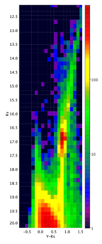
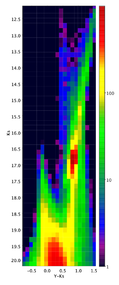
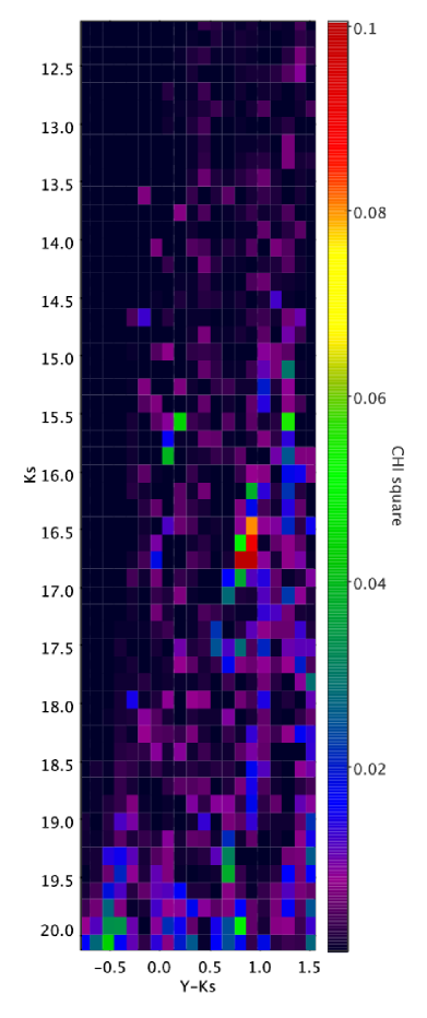
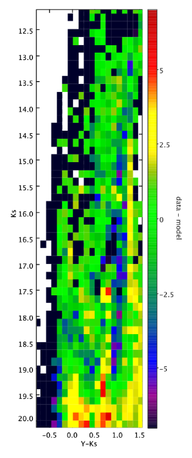
Figure 8: Examples of Hess diagrams obtained during a typical run of StarFISH – in this case, for subregion G1 of tile 8_3, with $\mbox{$(m\!-\!M)_{0}$}=18.48$ mag and $\mbox{$A_{V}$}=0.32$ mag. From left to right we show Hess diagrams for (a) the original VMC data, within the magnitude and colour limits used in this work, (b) the best-fitting model derived by StarFISH, (c) the $\chi^{2}$ map, that is the fractional contribution of each CMD bin to the total $\chi^{2}$, (d) the difference between data and best-fitting model. In panels (a), (b) and (d), the scale is in units of stars per CMD bin.

Using these SPMs we have recovered the SFH assuming a wide range in the values for $A_{V}$ and $(m\!-\!M)_{0}$. The $A_{V}$ vs. $(m\!-\!M)_{0}$ grid is regularly spaced by 0.03 mag and 0.025 mag, respectively, with limits: from 0.06 to 0.60 mag in $A_{V}$, in all three outer disk tiles; and from 18.40 to 18.55 mag in $(m\!-\!M)_{0}$ in tile 8_3, 18.40 to 18.53 in 4_3 and 18.28 to 18.50 in the 8_8 tile. For the 6_6 tile we used limits from 0.30 to 0.99 mag in $A_{V}$, and from 18.40 to 18.53 mag in $(m\!-\!M)_{0}$. The different limits reflect the fact that the different tiles are effectively found to be at different mean values of $A_{V}$ and $(m\!-\!M)_{0}$, as revealed by our initial explorative work using a much coarser grid of $A_{V}$ vs. $(m\!-\!M)_{0}$ values.

The SFH was recovered simultaneously using two CMDs, $K_{\rm s}$ vs. $J\!-\!K_{\rm s}$ with limits $-$0.52 to 0.88 mag in colour and 12.10 to 20.45 in magnitude, and $K_{\rm s}$ vs. $Y\!-\!K_{\rm s}$  with limits $-$0.82 to 1.56 mag in colour and 12.10 to 20.15 in magnitude. In tile 6_6 we used $\mbox{$K_{\rm s}$}=20$ mag as the faintest limit in all CMDs. These limits in colour and magnitude allow us to separate the LMC stars from most contaminating galaxies (see as an example Fig. 3 where most of the galaxies are clearly well separated up to $K_{s}=19.5$ mag and located in the faintest and redder part of the CMDs) and to derive the SFH using CMD regions with completeness greater than 70% in all cases.

The StarFISH code (Harris & Zaritsky 2001) is used to find the combination of SPMs that best fits the observed CMD, as illustrated in Fig. 8. The parameter describing the goodness-of-fit is the $\chi^{2}$-like statistic defined by Dolphin (2002). The final result of StarFISH are the weights of each partial model, which can be directly translated into the star formation rate (that is, the stellar mass formed per unit time, in $\mbox{$M_{\odot}$}\,{\rm yr}^{-1}$) as a function of lookback time, SFR$(t)$, and into a mean AMR, $\mbox{\rm[{\rm Fe}/{\rm H}]}(t)$ (see Kerber et al. 2009; Rubele et al. 2011, for details). We recall that StarFISH includes a method to drift outside of local minima in the parameter space (Harris & Zaritsky 2001), which we extensively tested using simulated VMC data (Kerber et al. 2009). Thus, we are quite confident that the SFH solutions we find are unique and the best-fitting ones.

Figures 9 to 12 show examples of the best-fitting ${\rm SFR}(t)$ and AMR (left panels), and the $\chi^{2}$ solution map as a function of $A_{V}$ and $(m\!-\!M)_{0}$ (right panels), in a subregion of each investigated tile. In the $\chi^{2}$ solution map, the black dashed and continuous lines illustrate the confidence error limit at $1\sigma$ and $3\sigma$, respectively.

In each one of these figures, the top left panel shows the $\mbox{${\rm SFR}(t)$}/\langle\mbox{${\rm SFR}(t)$}\rangle$ (blue histograms) with stochastic errors (blue errors bars) and the systematic ${\rm SFR}(t)$ variations inside the confidence level region of $1\sigma$ (gray shaded region). The middle left panels show the best-fitting AMR recovered (red and black points) together with its stochastic errors (red or black vertical bars). Red points show the median metallicity for when the ${\rm SFR}(t)$ reaches zero values inside its $3\sigma$ limit; black points are the same as red ones but for the cases in which the star formation is clearly detected, i.e. ${\rm SFR}(t)$ is non-zero inside the $3\sigma$ limit. The systematic AMR variations inside the $1\sigma$ confidence level are shown as the shaded region. The green points indicate the centres of the SPMs used for the recovery of the SFH (see Sect. 2). The bottom left panel illustrates the variation of the ${\rm SFR}(t)$ solution considering stochastic (dark violet line) and systematic errors (shaded regions).

We have completed the recovery of the SFH in 12 subregions in tiles 8_3, and 11 in 4_3, another 11 in 8_8, plus two small regions in 6_6. All results are illustrated in the Appendix. Subregions G9 in tiles 4_3 and 8_8 present photometry of lower quality, caused by the low $Y$ and $J$ sensitivity in the upper part of VIRCAM detector number 16. This effect is strong for these two bands for tile 4_3, which will not be further considered in this work. In tile 8_8 the effect is weak but could influence the SFH results, so we decided to show/use in this work only the derived parameters, distance modulus and extinction, but not the ${\rm SFR}(t)$ and AMR.

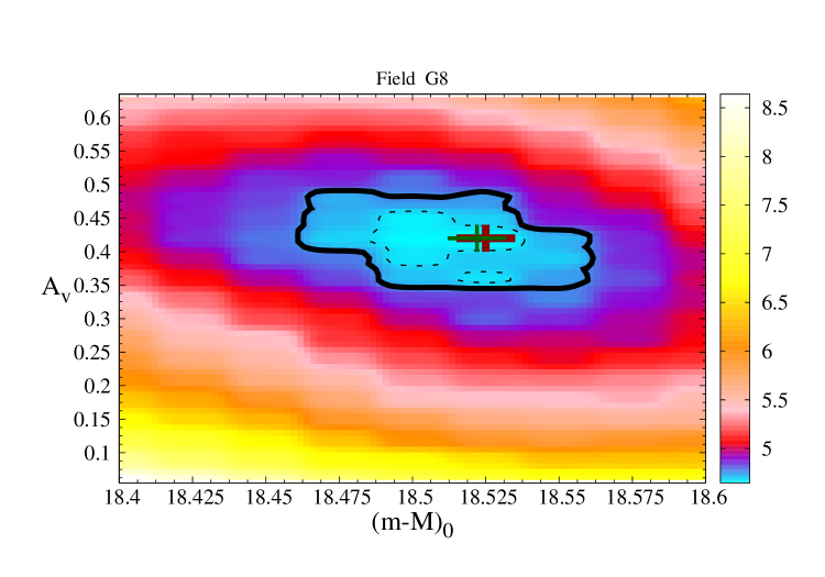
Figure 9: Example of the best-fitting solution in a subregion of tile 4_3. Left panel: The top part presents $\mbox{${\rm SFR}(t)$}/\langle\mbox{${\rm SFR}(t)$}\rangle$ (histograms) with stochastic errors (bars) and systematic variations (shaded regions) vs. $\log(t/{\rm yr})$. The central part shows the best-fitting AMR recovered (red and black points; red is used in age bins for which the ${\rm SFR}(t)$ is close to zero) with stochastic errors (red or black vertical bars) and systematic variations (shaded regions). The green dots indicate the central values of [Fe/H] and $\log(t/{\rm yr})$ of the SPMs. The bottom part shows the variation of the ${\rm SFR}(t)$ solution with stochastic errors (dashed line and bars) and systematic errors (shaded regions). Right panel: map of the $\chi^{2}$ values (as indicated by the colour scale) as a function of $A_{V}$ and $(m\!-\!M)_{0}$ with $1\sigma$ (dashed lines) and $3\sigma$ (continuous line) contours. The red cross marks the position of the best-fitting model. The green cross marks the position of the best model at the distance of the best-fitting LMC plane.

4 Distance modulus and extinction

As clearly illustrated in the right panels of Figs. 9 to 12, the SFH recovery provides estimates of the distance modulus and extinction, $(m\!-\!M)_{0}$ and $A_{V}$, for each subregion. These can be used to probe the LMC disk geometry, as well as to build reddening maps.

We evaluated the $A_{V}$ and $(m\!-\!M)_{0}$ values in each subregion as the average value inside the 68% confidence level (1$\sigma$) of the best-fitting solution, and its error from the width of this interval. Then, we compared our results with values obtained in Zaritsky et al. (2004) for the $A_{V}$ parameter, and Nikolaev et al. (2004), van der Marel & Cioni (2001), van der Marel et al. (2002), Olsen & Salyk (2002) and Subramanian & Subramaniam (2010) for $(m\!-\!M)_{0}$. Table 3 presents the results for all subregions considered. The parameters $A_{V}^{\rm CS}$ and $A_{V}^{\rm HS}$ are the $A_{V}$ values from Zaritsky et al. (2004) in the case of cool and hot stars, respectively, whereas $A_{V}^{\rm TW}$ and $(m\!-\!M)_{0}^{\rm TW}$ are the $A_{V}$ and $(m\!-\!M)_{0}$ values found in this work. In the table we also compare results for $(m\!-\!M)_{0}$ obtained in this work with those derived from geometric models of the LMC, namely: Nikolaev et al. (2004) in the case of $i=30.7^{\circ}$ and $\theta_{0}=151.0^{\circ}$ (where $i$ is the inclination and $\theta_{0}$ the position angle of line of nodes), and van der Marel & Cioni (2001) and van der Marel et al. (2002) with parameters $i=34.7^{\circ}$, $\theta_{0}=122.5^{\circ}$ and $\theta_{0}=129.9^{\circ}$, respectively.

Table 3: $(m\!-\!M)_{0}$ values obtained in this work: $(m\!-\!M)_{0}^{\rm TW}$ from the best-fitting SFH and $(m\!-\!M)_{0}^{\rm BFTW}$ from the best-fitting LMC disk. Also, $A_{V}$ values obtained in this work ($A_{V}^{\rm TW}$) compared to those from Zaritsky et al. (2004) for cool ($A_{V}^{\rm CS}$) and hot ($A_{V}^{\rm HS}$) stars.

Tile	Subregion	$\alpha$ (J2000)	$\delta$ (J2000)	$(m\!-\!M)_{0}^{\rm TW}$	$(m\!-\!M)_{0}^{\rm BFTW}$	$A_{V}^{\rm TW}$	$A_{V}^{\rm CS}$	$A_{V}^{\rm HS}$
		(deg)	(deg)	(mag)	(mag)	(mag)	(mag)	(mag)
4_3	G1	74.64	$-$72.62	$18.55\;(-0.03,+0.02)$	18.532	$0.219\;(-0.039,+0.021)$	0.42$\pm$0.32	0.73$\pm$0.43
	G2	74.81	$-$72.27	$18.52\;(-0.04,+0.03)$	18.527	$0.360\;(-0.090,+0.060)$	0.36$\pm$0.32	0.57$\pm$0.42
	G3	74.99	$-$71.92	$18.52\;(-0.02,+0.03)$	18.523	$0.295\;(-0.055,+0.064)$	0.43$\pm$0.32	0.50$\pm$0.37
	G4	75.16	$-$71.56	$18.50\;(-0.03,+0.02)$	18.518	$0.372\;(-0.042,+0.048)$	0.46$\pm$0.30	0.54$\pm$0.36
	G5	73.54	$-$72.57	$18.55\;(-0.01,+0.01)$	18.535	$0.372\;(-0.042,+0.048)$	0.66$\pm$0.34	0.87$\pm$0.37
	G6	73.73	$-$72.22	$18.53\;(-0.01,+0.02)$	18.530	$0.440\;(-0.050,+0.040)$	0.62$\pm$0.32	0.84$\pm$0.38
	G7	73.93	$-$71.87	$18.53\;(-0.01,+0.02)$	18.526	$0.354\;(-0.054,+0.036)$	0.42$\pm$0.30	0.62$\pm$0.41
	G8	74.11	$-$71.51	$18.51\;(-0.01,+0.01)$	18.521	$0.410\;(-0.050,+0.040)$	0.48$\pm$0.29	0.52$\pm$0.38
	G10	72.67	$-$72.16	$18.54\;(-0.02,+0.03)$	18.533	$0.240\;(-0.060,+0.060)$	0.60$\pm$0.32	0.89$\pm$0.41
	G11	72.87	$-$71.81	$18.55\;(-0.03,+0.02)$	18.529	$0.440\;(-0.081,+0.069)$	0.45$\pm$0.31	0.74$\pm$0.40
	G12	73.08	$-$71.45	$18.55\;(-0.03,+0.02)$	18.524	$0.373\;(-0.073,+0.077)$	0.59$\pm$0.34	0.66$\pm$0.38
6_6	D1	85.64	$-$69.92	$18.43\;(-0.05,+0.02)$	18.456	$0.650\;(-0.056,+0.033)$	0.50$\pm$0.38	0.68$\pm$0.42
	D2	83.27	$-$68.81	$18.44\;(-0.01,+0.01)$	18.450	$0.600\;(-0.040,+0.050)$	0.44$\pm$0.34	0.55$\pm$0.39
8_3	G1	76.90	$-$66.83	$18.48\;(-0.03,+0.05)$	18.453	$0.286\;(-0.016,+0.043)$	0.45$\pm$0.32	0.57$\pm$0.44
	G2	77.00	$-$66.48	$18.44\;(-0.01,+0.04)$	18.448	$0.321\;(-0.051,+0.038)$	0.38$\pm$0.30	0.52$\pm$0.46
	G3	77.10	$-$66.13	$18.44\;(-0.04,+0.03)$	18.443	$0.324\;(-0.054,+0.095)$	0.35$\pm$0.26	0.49$\pm$0.41
	G4	77.20	$-$65.77	$18.47\;(-0.02,+0.05)$	18.438	$0.237\;(-0.057,+0.032)$	0.39$\pm$0.28	0.54$\pm$0.41
	G5	76.09	$-$66.80	$18.44\;(-0.02,+0.03)$	18.456	$0.360\;(-0.030,+0.030)$	0.41$\pm$0.32	0.54$\pm$0.45
	G6	76.19	$-$66.44	$18.42\;(-0.03,+0.03)$	18.451	$0.372\;(-0.042,+0.048)$	0.38$\pm$0.28	0.48$\pm$0.46
	G7	76.29	$-$66.09	$18.44\;(-0.04,+0.04)$	18.446	$0.360\;(-0.030,+0.030)$	0.33$\pm$0.26	0.45$\pm$0.41
	G8	76.40	$-$65.74	$18.45\;(-0.05,+0.03)$	18.441	$0.366\;(-0.066,+0.053)$	0.40$\pm$0.30	0.52$\pm$0.41
	G9	75.25	$-$66.76	$18.45\;(-0.03,+0.02)$	18.460	$0.420\;(-0.030,+0.030)$	0.37$\pm$0.26	0.63$\pm$0.48
	G10	75.38	$-$66.40	$18.46\;(-0.02,+0.04)$	18.455	$0.276\;(-0.066,+0.054)$	0.33$\pm$0.26	0.51$\pm$0.48
	G11	75.50	$-$66.05	$18.42\;(-0.03,+0.05)$	18.450	$0.412\;(-0.082,+0.067)$	0.34$\pm$0.28	0.39$\pm$0.43
	G12	75.62	$-$65.70	$18.44\;(-0.04,+0.03)$	18.445	$0.303\;(-0.093,+0.057)$	0.33$\pm$0.27	0.54$\pm$0.46
8_8	G1	90.83	$-$66.86	$18.40\;(-0.05,+0.05)$	18.389	$0.239\;(-0.118,+0.121)$	0.25$\pm$0.20	0.67$\pm$0.49
	G2	90.73	$-$66.51	$18.38\;(-0.06,+0.04)$	18.384	$0.238\;(-0.117,+0.122)$	0.31$\pm$0.23	0.83$\pm$0.45
	G3	90.64	$-$66.16	$18.35\;(-0.05,+0.05)$	18.379	$0.202\;(-0.111,+0.128)$	0.35$\pm$0.26	0.92$\pm$0.43
	G4	90.55	$-$65.81	$18.35\;(-0.05,+0.05)$	18.375	$0.188\;(-0.067,+0.082)$	0.40$\pm$0.26	0.95$\pm$0.41
	G5	89.99	$-$66.90	$18.40\;(-0.02,+0.03)$	18.393	$0.198\;(-0.077,+0.072)$	0.27$\pm$0.22	0.60$\pm$0.50
	G6	89.90	$-$66.54	$18.38\;(-0.05,+0.03)$	18.388	$0.213\;(-0.062,+0.087)$	0.31$\pm$0.25	0.77$\pm$0.47
	G7	89.81	$-$66.19	$18.39\;(-0.04,+0.04)$	18.384	$0.173\;(-0.053,+0.066)$	0.36$\pm$0.27	0.84$\pm$0.45
	G8	89.73	$-$65.84	$18.41\;(-0.04,+0.04)$	18.379	$0.176\;(-0.085,+0.064)$	0.39$\pm$0.25	0.90$\pm$0.44
	G10	89.08	$-$66.57	$18.39\;(-0.02,+0.01)$	18.393	$0.186\;(-0.036,+0.024)$	0.36$\pm$0.29	0.76$\pm$0.47
	G11	89.00	$-$66.22	$18.41\;(-0.01,+0.01)$	18.388	$0.146\;(-0.055,+0.034)$	0.36$\pm$0.27	0.77$\pm$0.41
	G12	88.93	$-$65.87	$18.41\;(-0.04,+0.04)$	18.383	$0.100\;(-0.040,+0.050)$	0.40$\pm$0.28	0.81$\pm$0.48

4.1 Fitting the LMC disk plane

For all the 36 subregions (see Table 3) distributed in four VMC tiles in which we have derived the SFH, we obtain independent determinations of the distance modulus and reddening. The good accuracy of each distance determination allows us to fit a disk plane geometry to the LMC disk. To perform this fit we considered the following five free parameters: the equatorial coordinates for the LMC centre, ${\alpha_{\rm c}}$ and ${\delta_{\rm c}}$; the distance modulus to the LMC centre, $(m\!-\!M)_{0}^{\rm centre}$; the disk inclination on the plane of the sky, $i$ (where $i=0^{\circ}$ means a face-on disk); and the position angle of the line of nodes, $\theta_{0}$.

In practice, to fit the LMC disk plane we used four different choices for (${\alpha_{\rm c}}$, ${\delta_{\rm c}}$) in accordance with previous determinations of the LMC disk geometry proposed by different authors (Table 4). This procedure simplified the search for the best-fitting plane, and allowed us to check the dependence of the results for the remaining three parameters with the adopted coordinates for the LMC centre.

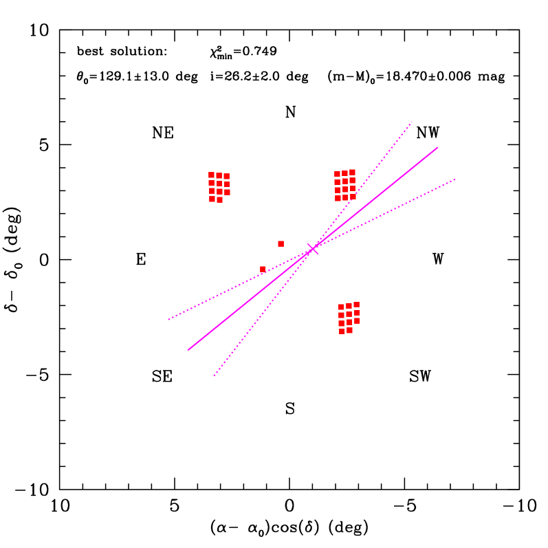
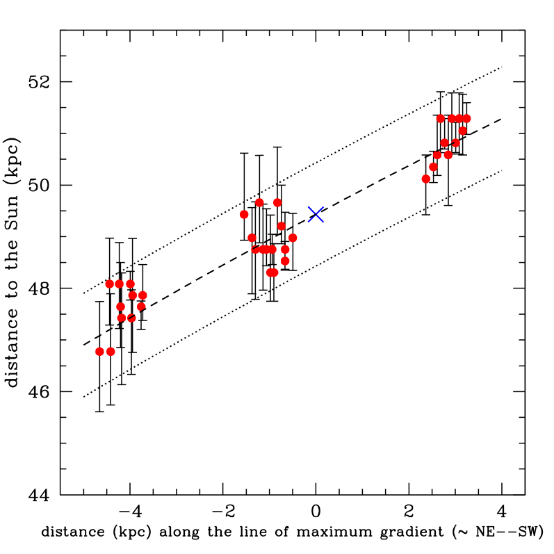
Figure 13: Best-fitting model of the LMC disk using as centre of the LMC the coordinates derived by Nikolaev et al. (2004, cross). Left panel: the line of nodes (solid line) and the 36 tile subregions (red squares) as projected on the sky. The disk parameters are shown in the figure, as well as the uncertainties in the position angle of the line of nodes (dotted lines). Right panel: distance to these subregions projected onto the line perpendicular to the line of nodes, i.e. the line of the maximum LMC disk gradient ($\sim$ NE–SW direction).

Figure 13 illustrates the best-fitting model for a specific choice for (${\alpha_{\rm c}}$,${\delta_{\rm c}}$), in this case that adopted by Nikolaev et al. (2004). The left panel shows the results of the LMC disk as projected on the sky, whereas the right panel presents the projection along the line perpendicular to the line of nodes, i.e., the line of the maximum gradient for the LMC disk. As can be seen in this figure, all fields studied so far are fit extremely well by a single disk with the following parameters: $i=26.2\pm 2.0^{\circ}$, $\theta_{0}=129.1\pm 13.0^{\circ}$ and $\mbox{$(m\!-\!M)_{0}^{\rm centre}$}=18.470\pm 0.006$ mag. The errors in each parameter correspond to the 68% confidence level, and are computed using the bootstrapping technique, where 50 resamples (for the set of $(m\!-\!M)_{0}$ values) are generated while accounting for the individual errors in each measurement. Table 5 summarizes the final results for the LMC disk geometry, revealing that these results are quite insensitive to the adopted (${\alpha_{\rm c}}$, ${\delta_{\rm c}}$) values. A comparison between Tables 4 and 5 shows that we recover a disk significantly less inclined than other authors, who tend to find $i$ values close to $\sim 35^{\circ}$ (with the exception of one value from Subramanian & Subramaniam 2010). Regarding $\theta_{0}$, our values are well inside the wide range – from $122.5^{\circ}$ to $163.7^{\circ}$ – found in the literature.

The distances we recover to the LMC centre, $(m\!-\!M)_{0}^{\rm centre}$, are in good agreement with most of the determinations in the recent past, which as demonstrated by Schaefer (2008), tend to cluster extremely well (and suspiciously well, from a statistical point of view) around the value of $\mbox{$(m\!-\!M)_{0}$}=18.50\pm 0.10$ mag adopted by the HST Key Project on the distance scale (Freedman et al. 2001). Regarding our distance determinations, we recall that they are derived in an objective way from the global fitting of the CMD, and not from any particular set of favoured distance indicators. Despite the good agreement with the “standard” distance values, we recognize that this particular result could be affected by systematic errors in the stellar evolution models and/or photometric ZPs, and should be verified by means of independent methods. This is beyond the scope of the present work. Forthcoming papers will use different distance indicators on VMC data (in particular the RR Lyrae and red clump stars), to further discuss this issue.

Table 4: LMC disk parameters from the literature.

${\alpha_{\rm c}}$ (J2000)	${\delta_{\rm c}}$ (J2000)	$i$	$\theta_{0}$	Reference	distance indicator
(deg)	(deg)	(deg)	(deg)
79.40	$-$69.03	$30.7\pm 1.1$	$151.0\pm 2.4$	Nikolaev et al. (2004)	Cepheids (MACHO + 2MASS)
82.25	$-$69.50	$34.7\pm 6.2$	$122.5\pm 8.3$	van der Marel & Cioni (2001)	AGB stars (DENIS + 2MASS)
81.90	$-$69.87	$34.7\pm 6.2^{*}$	$129.9\pm 6.0$	van der Marel et al. (2002)	carbon stars (kinematics)
79.91	$-$69.45	$35.8\pm 2.4$	$145\pm 4$	Olsen & Salyk (2002)	red clump (CTIO 0.9m $VI$ photom.)
79.91	$-$69.45	$23.0\pm 0.8$	$163.7\pm 1.5$	Subramanian & Subramaniam (2010)	red clump (OGLE III $VI$ photom.)
79.91	$-$69.45	$37.4\pm 2.3$	$141.2\pm 3.7$	Subramanian & Subramaniam (2010)	red clump (MCPS $VI$ photom.)

^∗Fixed to the van der Marel & Cioni (2001) value.

Table 5: Our best-fitting models for the LMC disk, for different choices of ${\alpha_{\rm c}}$ and ${\delta_{\rm c}}$.

${\alpha_{\rm c}}$(J2000)	${\delta_{\rm c}}$(J2000)	$i$	$\theta_{0}$	$(m\!-\!M)_{0}^{\rm centre}$	$\chi^{2}_{\rm{min}}$
(deg)	(deg)	(deg)	(deg)
79.40	$-$69.03	$26.2\pm 2.0$	$129.1\pm 13.0$	$18.470\pm 0.006$	0.749
82.25	$-$69.50	$26.2\pm 1.9$	$126.4\pm 10.1$	$18.466\pm 0.006$	0.785
81.90	$-$69.87	$26.2\pm 2.0$	$130.9\pm 8.9$	$18.470\pm 0.005$	0.750
79.91	$-$69.45	$26.2\pm 1.7$	$129.6\pm 10.1$	$18.471\pm 0.006$	0.769

4.2 Extinction values

The spatial resolution adopted in the present work is too coarse to allow the derivation of detailed extinction maps. However, a first comparison with other works is advisable for the sake of validating our results, and is particularly interesting because previous extinction maps are mainly based on optical data.

Table 3 presents the $A_{V}$ values derived in this work, $A_{V}^{\rm TW}$, in comparison to those derived from the Magellanic Cloud Photometric Survey (MCPS) data by Zaritsky et al. (2004), in the case of cool and hot stars ($A_{V}^{\rm CS}$ and $A_{V}^{\rm HS}$, respectively). Note that our results represent mean values for an entire subregion, in contrast to the star-by-star values derived by Zaritsky et al. (2004). This explains why their error bars are intrinsically much longer.

In regions with low stellar density, our $A_{V}$ values are much smaller than those of Zaritsky et al. (2004), in particular if we consider the $A_{V}^{\rm HS}$. Better agreement is present if we consider denser regions, in particular in the two subregions of the 6_6 tile. We note that Haschke et al. (2011) find a similar discrepancy between their $A_{V}$ values, derived from both the red clump and RR Lyrae $V\!-\!I$ colours from OGLE III data, and those from Zaritsky et al. (2004). Haschke et al. (2011) obtained, for a wide area over the LMC, a mean colour excess $\mbox{$E_{V\!-\!I}$}=0.09\pm 0.07$ mag that translates into $\mbox{$A_{V}$}=0.22\pm 0.17$ mag, in good general agreement with our values. The reddening issue will be further discussed in a forthcoming VMC paper.

5 Discussion and conclusions

5.1 Reducing SFH errors

We have recovered the SFH in four VMC tiles across the LMC evaluating simultaneously their best-fitting ${\rm SFR}(t)$, AMR, $A_{V}$ and $(m\!-\!M)_{0}$, and their stochastic and systematic errors inside the 68% confidence level in each subregion for each tile. We find clear indications that these LMC regions are distributed, to a first approximation, across a single disk plane.

We can take advantage of this latter conclusion to further improve the SFH results. Indeed, the uncertainties in both $(m\!-\!M)_{0}$ and $A_{V}$ contribute to the systematic errors in the derived ${\rm SFR}(t)$ and AMR. If we assume that this distance is exactly known and defined by the best-fitting disk, only the range of $A_{V}$ values is left to be explored, and the errors are expected to decrease. We therefore make this assumption of a known distance, given by the plane defined in the first row of Table 4, for each subregion in each tile. SFH-recovery is re-done by exploring the same range of $A_{V}$ values as before, while the errors are re-computed.

Figure 14 illustrates the typical results of this exercise. Note that, in addition to illustrating the effect of assuming a known distance, the figure also presents the total results added over all subregions in a tile – in this case, the 8_8 tile. The same general features are observed in every single subregion we examined.

It is striking in Fig. 14 that in both cases (with unknown/known distance) we derive about the same mean ${\rm SFR}(t)$ and AMR, but the error bars are significantly reduced when the distance is known. For the oldest age bins, the error bars are reduced by a factor of about 2. This exercise clearly indicates the potential of exploring the SFH over wide areas in the LMC: we can take advantage of known correlations between parameters over large scales (in this case, $(m\!-\!M)_{0}$), to improve the SFH obtained in small regions of the galaxy.

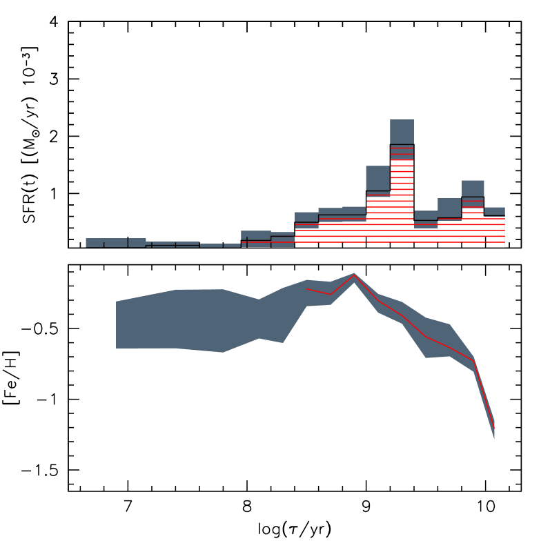
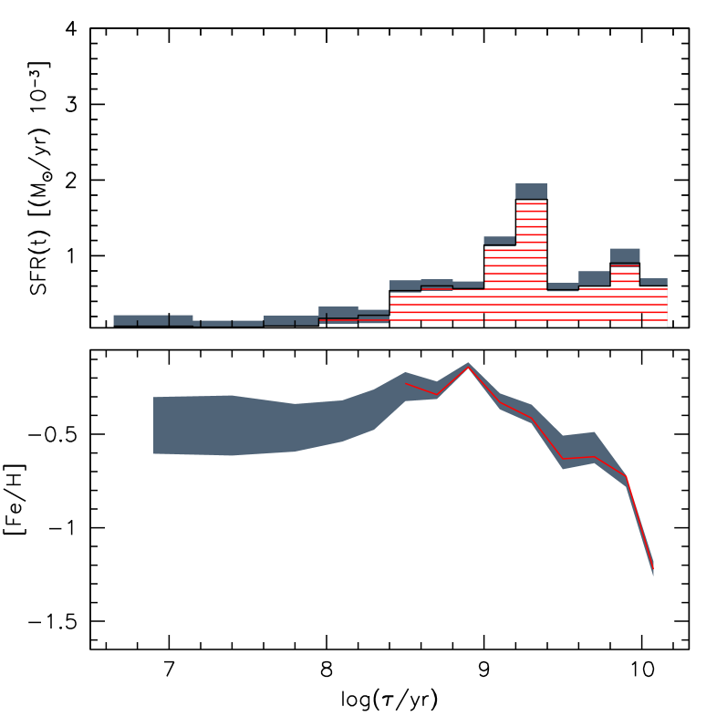
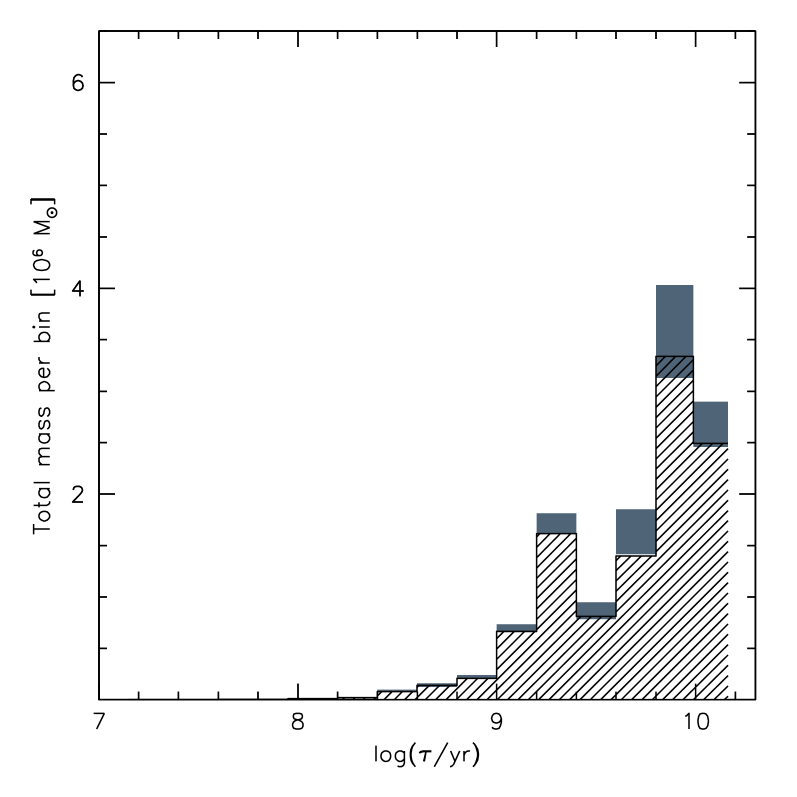
Figure 14: Total ${\rm SFR}(t)$ and AMR derived for tile 8_8, resulting from the addition of the SFH values for all subregions. Left panels: The ${\rm SFR}(t)$ as a function of $\log(t/{\rm yr})$ (red shaded histogram) and its systematic variations (gray), together with the mean AMR in all age bins in which the ${\rm SFR}(t)$ is non-negligible (red line) and its systematic variations (gray). These results are obtained assuming that both $(m\!-\!M)_{0}$ and $A_{V}$ are free parameters. The middle panels show the same but using a fixed $(m\!-\!M)_{0}$ – obtained from the best-fitting disk geometry – and assuming that only $A_{V}$ is a free parameter. The right panel shows the total stellar mass formed inside each $\log(t/{\rm yr})$ bin (shaded histogram) together with the systematic variations (gray area).

5.2 The stellar mass formation history

In the following subsections we comment on the global results for each tile, starting from those with the best photometry. Before doing that, we call attention to the rightmost panels in Figs. 14–17, which show the distribution of total mass of formed stars along the age bins defined in this work. These plots indicate that the star formation at young ages represents, as a rule, just a minor fraction of the total stellar mass formed in the LMC. For all tiles studied so far, most of the star formation has occurred at ages $\mbox{$\log(t/{\rm yr})$}\!>\!9.5$ ($t\!>\!3$ Gyr), whereas just $\la\!9$ % has occurred at ages $\mbox{$\log(t/{\rm yr})$}<9.0$. Therefore, even strong peaks detected with high significance in the ${\rm SFR}(t)$ at young ages, may not represent major events in the formation of stellar mass in the LMC.

Another remarkable feature in these panels is the modest size of the systematic errors, especially at the oldest age bins where one could have expected them to be significant because of the incompleteness and larger photometric errors at the level of the oldest MSTOs. Instead, both random and systematic errors keep modest because of the large numbers of stars sampled by VMC, as anticipated by Kerber et al. (2009). Summing the values in the right panels in Fig. 14–17, one can estimate the total stellar mass formed for every analised region of the LMC, with errors of just $\la\!20$ %. The main limitation of these estimates are ptobably in the uncertainties in the initial mass function, which determines the fraction of total mass going into faint, undetectable main sequence stars.

5.3 Tile 8_8

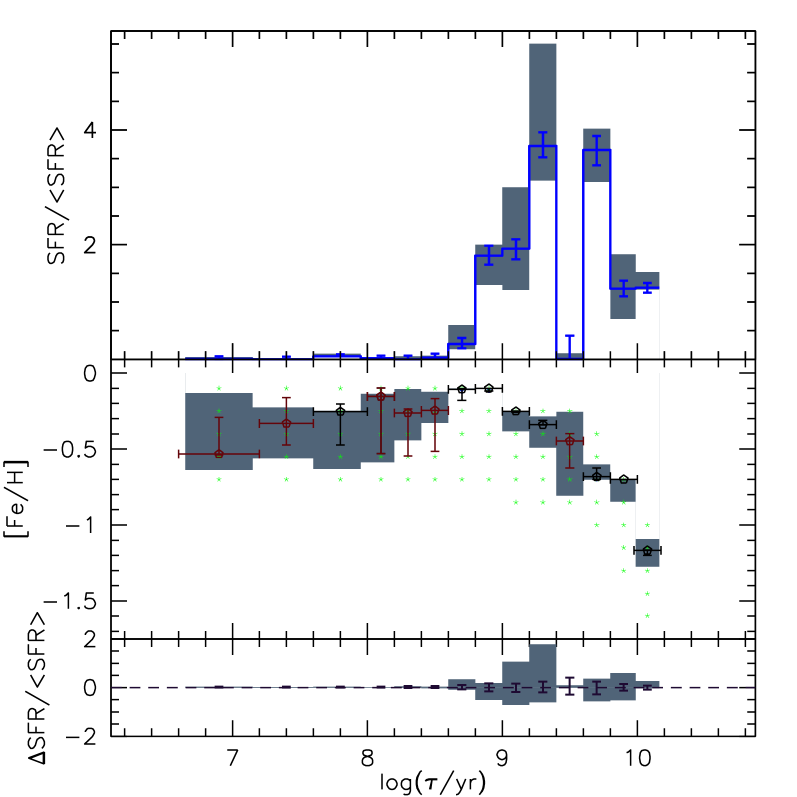
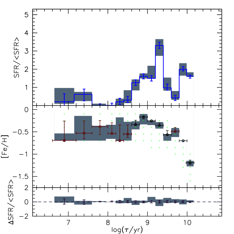
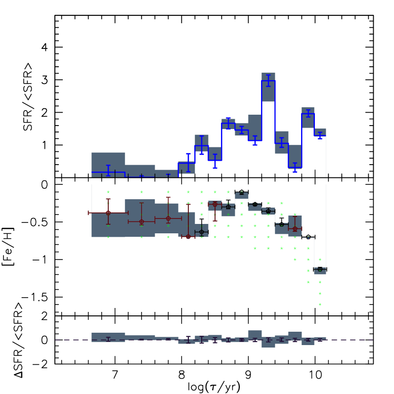
(a) ${\rm SFR}(t)$ and AMR of subregions G4, G8, and G12

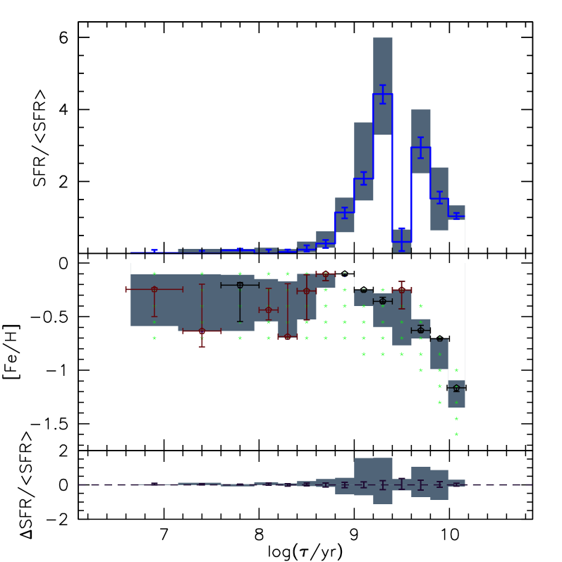
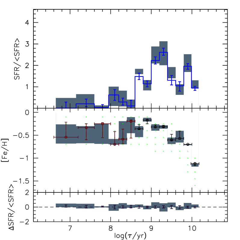
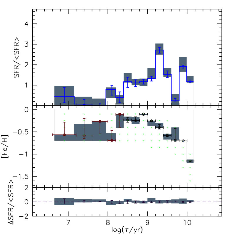
(b) ${\rm SFR}(t)$ and AMR of subregions G3, G7 and G11

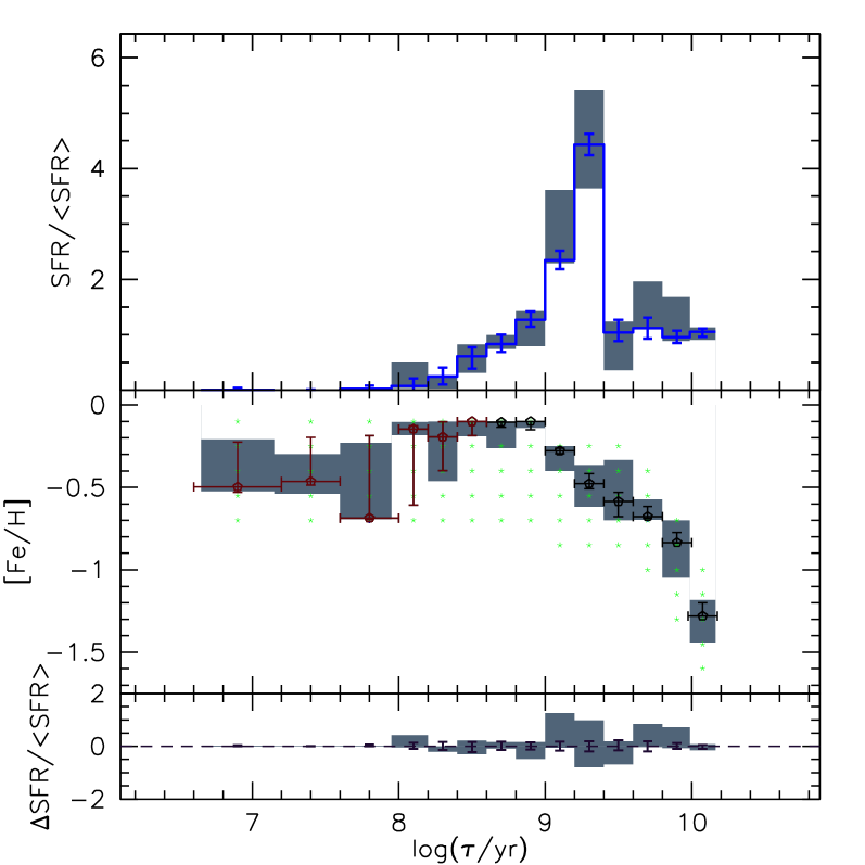
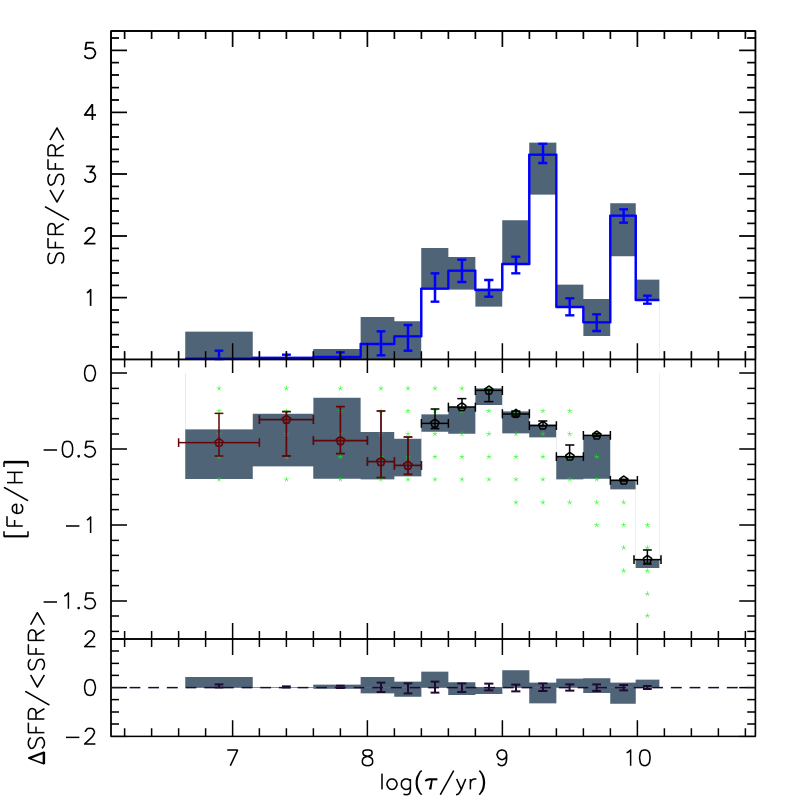
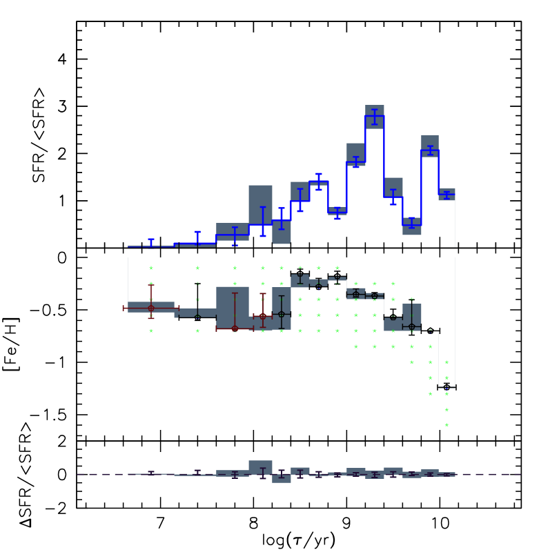
(c) ${\rm SFR}(t)$ and AMR of subregions G2, G6 and G10

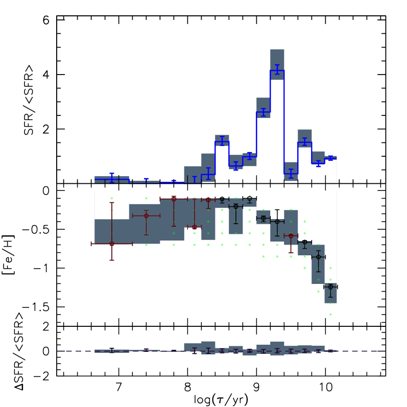
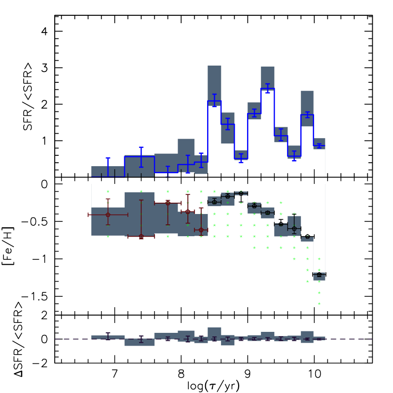
(d) ${\rm SFR}(t)$ and AMR of subregions G1 and G5

Figure 18: SFH for the subregions of the 8_8 tile. The panel are disposed in the same way as seen in the sky, with North to the top and West to the right (see Fig. 2). The bottom right panels represent subregions closer to the LMC centre.

This tile represents on average $\mbox{$A_{V}$}\!\sim\!0.2$ mag and $\mbox{$(m\!-\!M)_{0}$}\!\sim\!18.39$ mag. Considering old stellar populations, the ${\rm SFR}(t)$ (Fig. 14) is similar from subregion to subregion. This is more evident comparing the different panels in Fig. 18. In addition to the oldest star formation detected at $\mbox{$\log(t/{\rm yr})$}>10.0$, which appears with $\mbox{\rm[{\rm Fe}/{\rm H}]}\!\sim\!-1.0$ dex, it is possible to see evidence for two other main star formation (SF) episodes:

1. The first happened at $\mbox{$\log(t/{\rm yr})$}=9.9$ and has $\mbox{\rm[{\rm Fe}/{\rm H}]}\!\sim\!-0.70$ dex. It may have formed up to 31 % of the total stellar mass in this tile.

2. The second is more recent and occurred between $\mbox{$\log(t/{\rm yr})$}=9.1$ and 9.3, with an average $\mbox{\rm[{\rm Fe}/{\rm H}]}\!\sim\!-0.42$ dex. This metallicity coincides with the values found in LMC intermediate age clusters of similar age (Kerber et al. 2007; Olszewski et al. 1991; Mackey & Gilmore 2003; Grocholski et al. 2006). Although it appears as a very prominent peak in the ${\rm SFR}(t)$ plot (left and middle panels), it represents just 21 % of the total mass formed in this tile (right panel).

In addition, examination of Fig. 18 reveals the presence of a third peak in the ${\rm SFR}(t)$ at $\mbox{$\log(t/{\rm yr})$}=8.5-8.7$ , which is well evident only in subregions G1, G5, G6, and marginally seen also in G7, G10, G11 and G12. These are also the innermost subregions of this tile. Therefore, there is a clear indication that this more recent SF episode did not occur outside of a given radius in the LMC disk.

The SF for ages less than $\mbox{$\log(t/{\rm yr})$}=8.3$ seems to be negligible in this tile. It was not possible to evaluate the AMR of the youngest stellar populations, because of the very low ${\rm SFR}(t)$ at all ages $\mbox{$\log(t/{\rm yr})$}<8.3$.

5.4 Tile 8_3

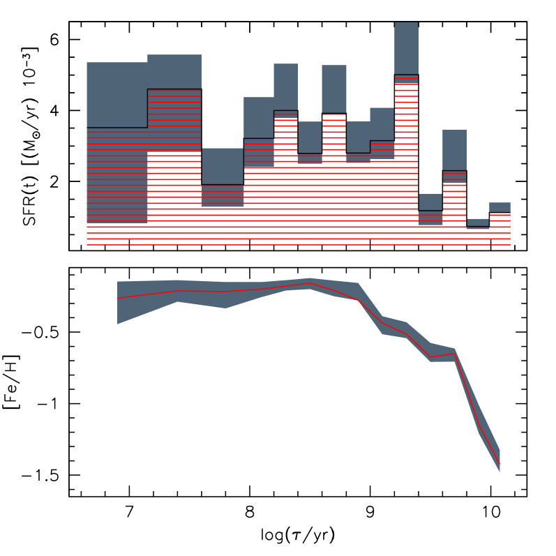
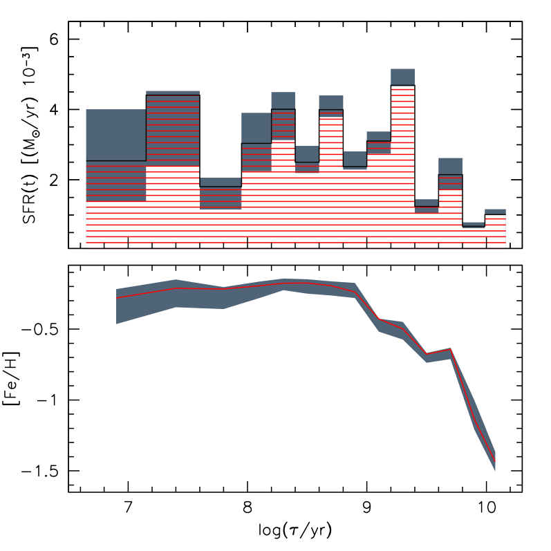
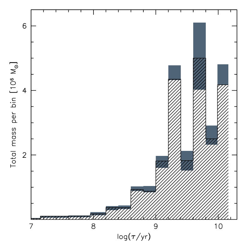
Figure 15: Total ${\rm SFR}(t)$ and AMR in tile 8_3. Colours and lines are as in Fig. 14.

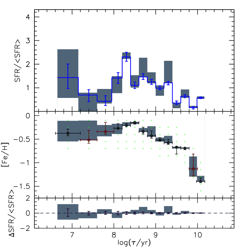
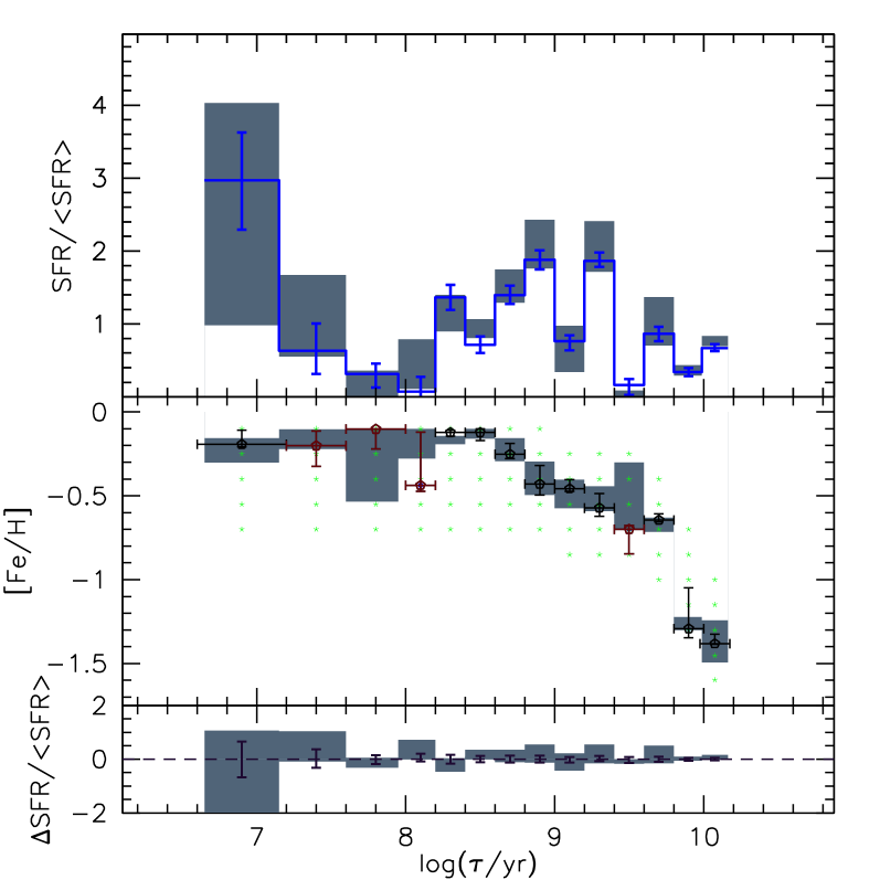
(a) ${\rm SFR}(t)$ and AMR of subregions G4, G8 and G12

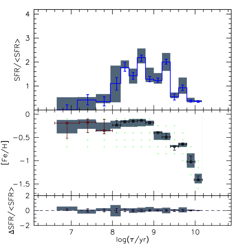
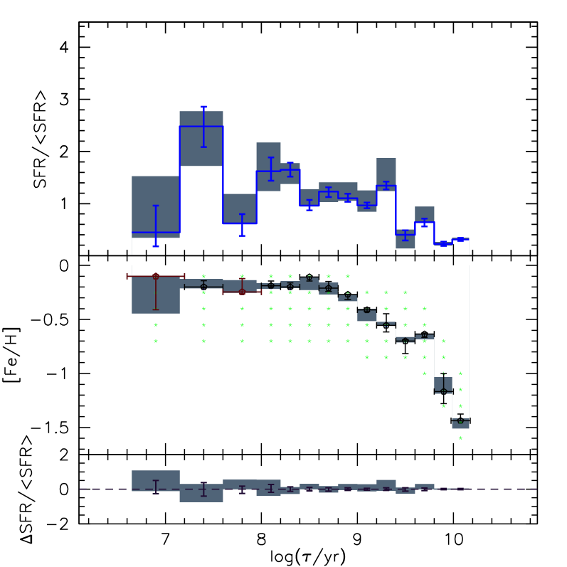
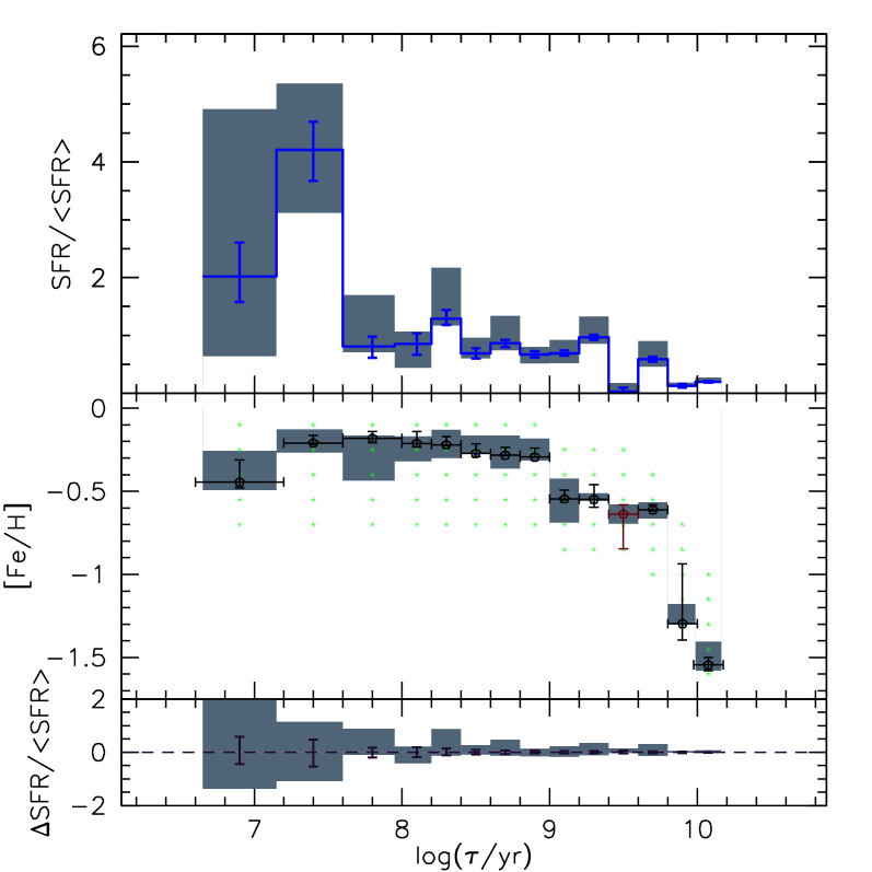
(b) ${\rm SFR}(t)$ and AMR of subregions G3, G7 and G11

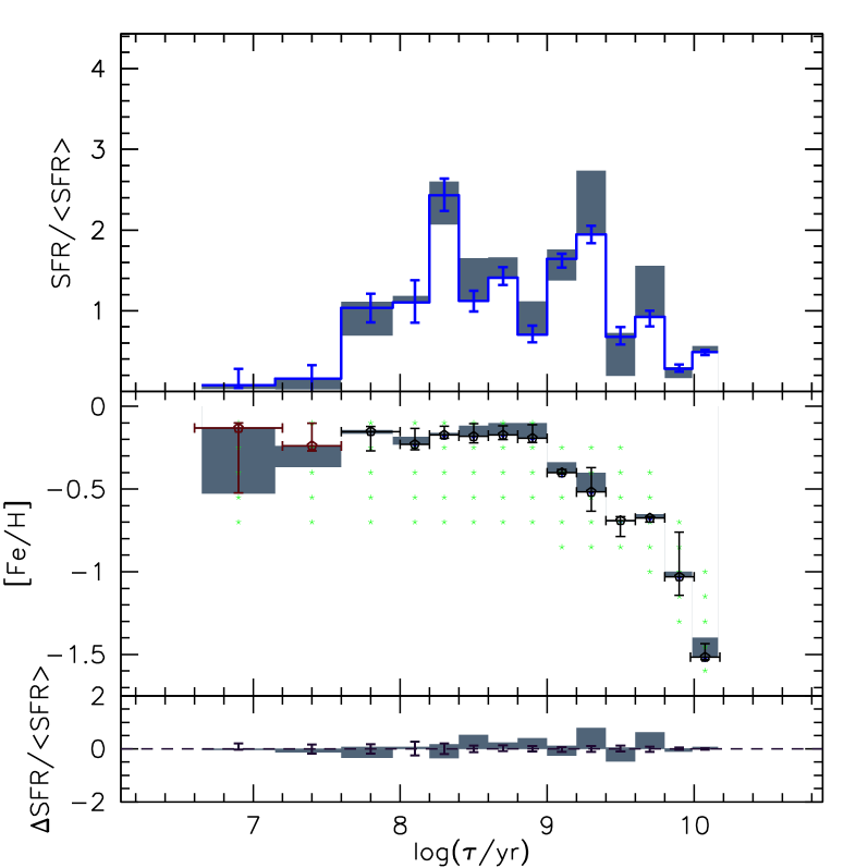
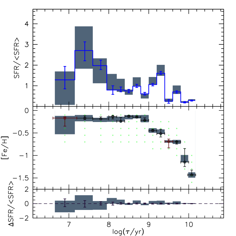
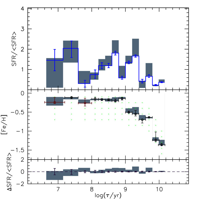
(c) ${\rm SFR}(t)$ and AMR of subregions G2, G6 and G10

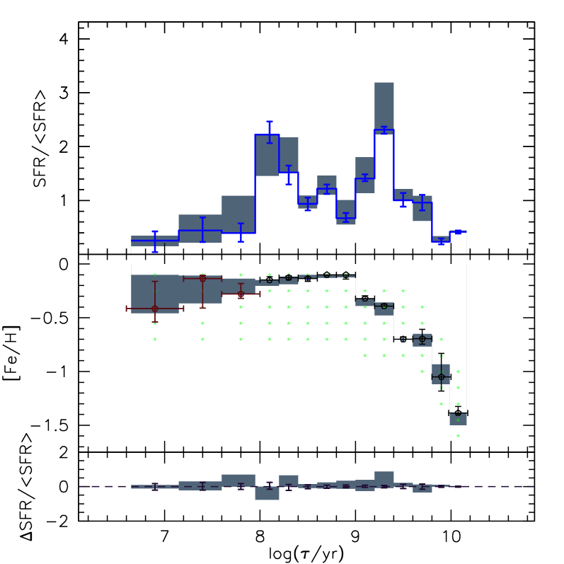
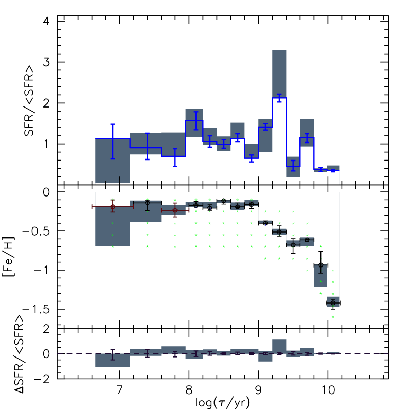
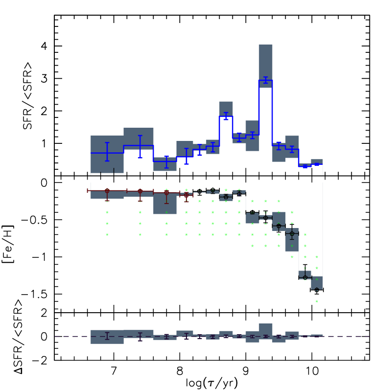
(d) ${\rm SFR}(t)$ and AMR of subregions G1, G5 and G9

Figure 19: Same as in Fig. 18, but for the SFH for the 8_3 tile. The bottom left panels represent subregions closer to the LMC centre.

In this tile the typical $A_{V}$ and $(m\!-\!M)_{0}$ values are $\sim\!0.33$ and $\sim\!18.45$ mag, respectively. Fig. 15 shows the total ${\rm SFR}(t)$ and AMR in the same way as for tile $8\_8$. Note the prominent, and almost constant ${\rm SFR}(t)$ over the most recent couple of Gyr. This young SF changes significantly from subregion to subregion, as revealed by Fig. 19. SF for ages $\mbox{$\log(t/{\rm yr})$}<8$ is present in most of the subregions in the West part of this tile (from G5 to G12), although with large error bars. This recent ${\rm SFR}(t)$ can be associated to the presence of gas in the proximity of N11, the second-most most proficient star-forming region in the LMC, which falls next to the Western border of the 8_3 tile.

As for the tile 8_8, in addition to the oldest star formation detected at $\mbox{$\log(t/{\rm yr})$}>10.0$ with $\mbox{\rm[{\rm Fe}/{\rm H}]}\!\sim\!-1.0$ dex, it is also possible to identify two main SF episodes:

1. The first at $\mbox{$\log(t/{\rm yr})$}=9.7$ and with a $\mbox{\rm[{\rm Fe}/{\rm H}]}\!\sim\!-0.65$ dex, which formed 22 % of the stellar mass.

2. The second between $\mbox{$\log(t/{\rm yr})$}=9$ and 9.4 and with an average $\mbox{\rm[{\rm Fe}/{\rm H}]}\!\sim\!-0.47$ dex, forming about 27 % of the stellar mass.

The total AMR seems to change little from subregion to subregion (see Fig. 19), and shows small variations also for the young stellar population.

5.5 Tile 4_3

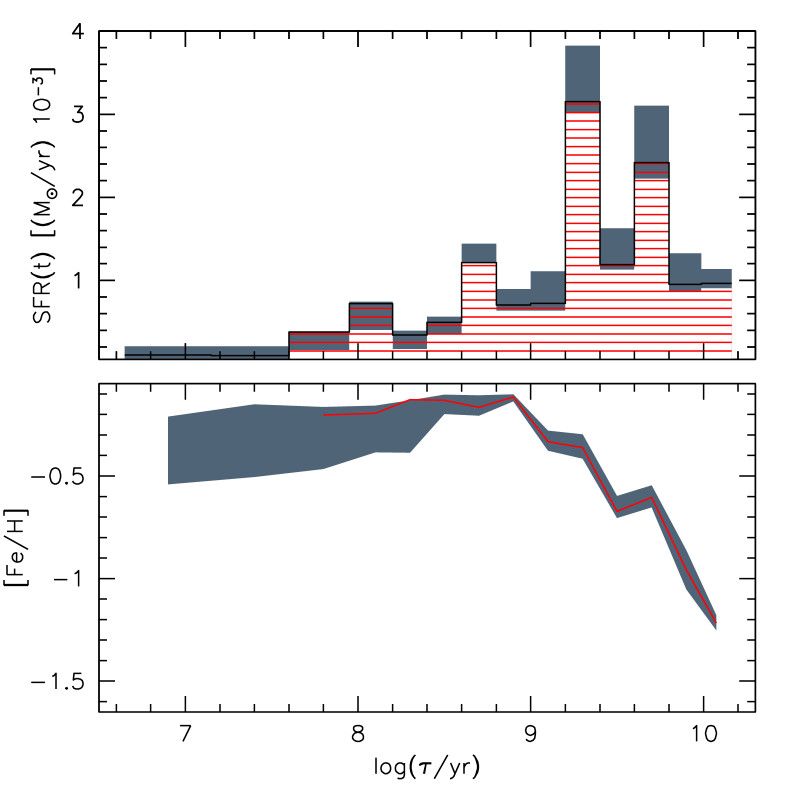
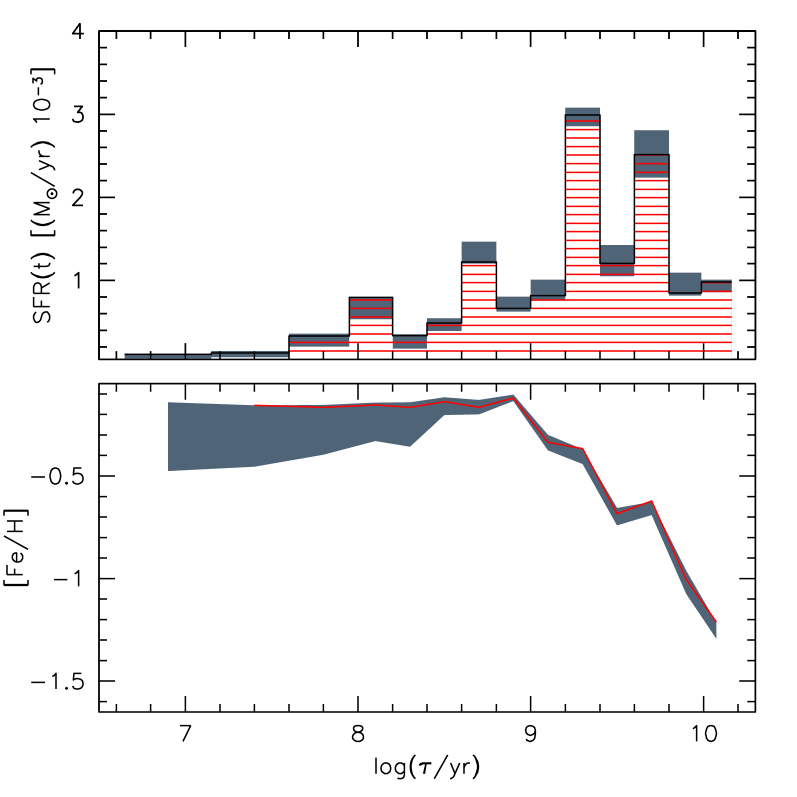
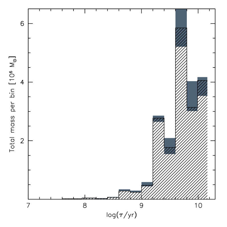
Figure 16: Total ${\rm SFR}(t)$ and AMR in tile 4_3. Colours and lines are as in figure 14.

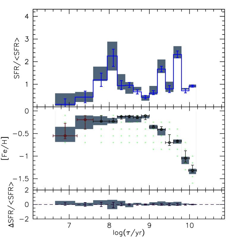
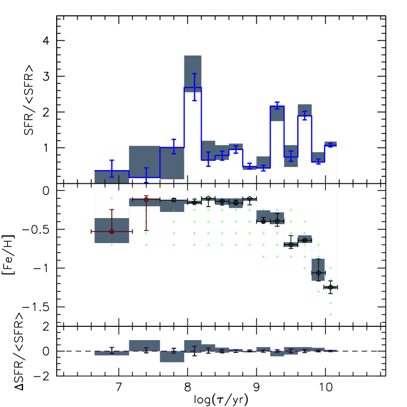
(a) ${\rm SFR}(t)$ and AMR of subregions G4, G8 and G12

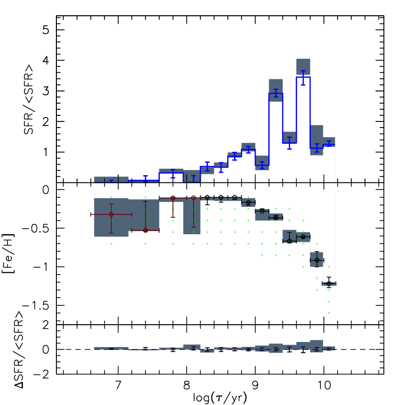
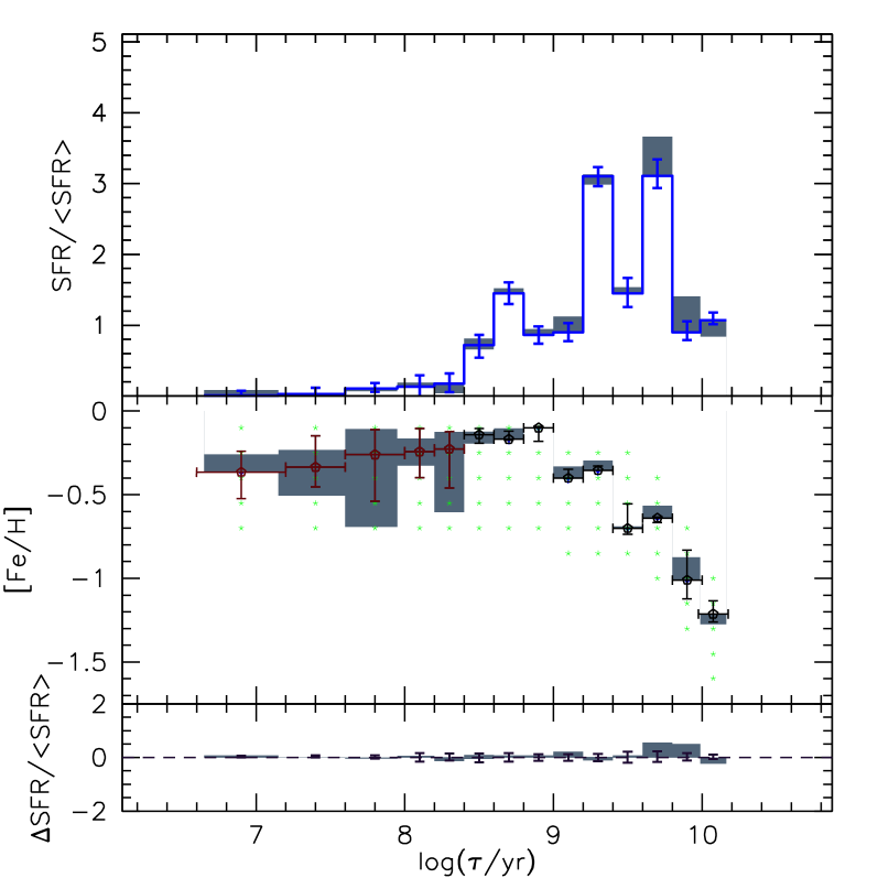
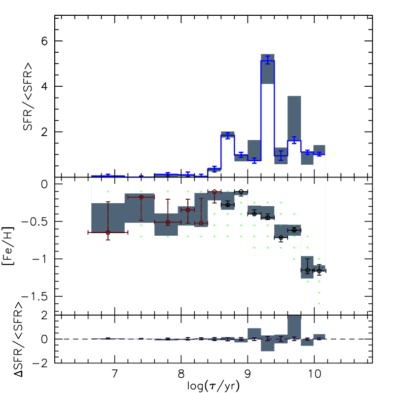
(b) ${\rm SFR}(t)$ and AMR of subregions G3, G7 and G11

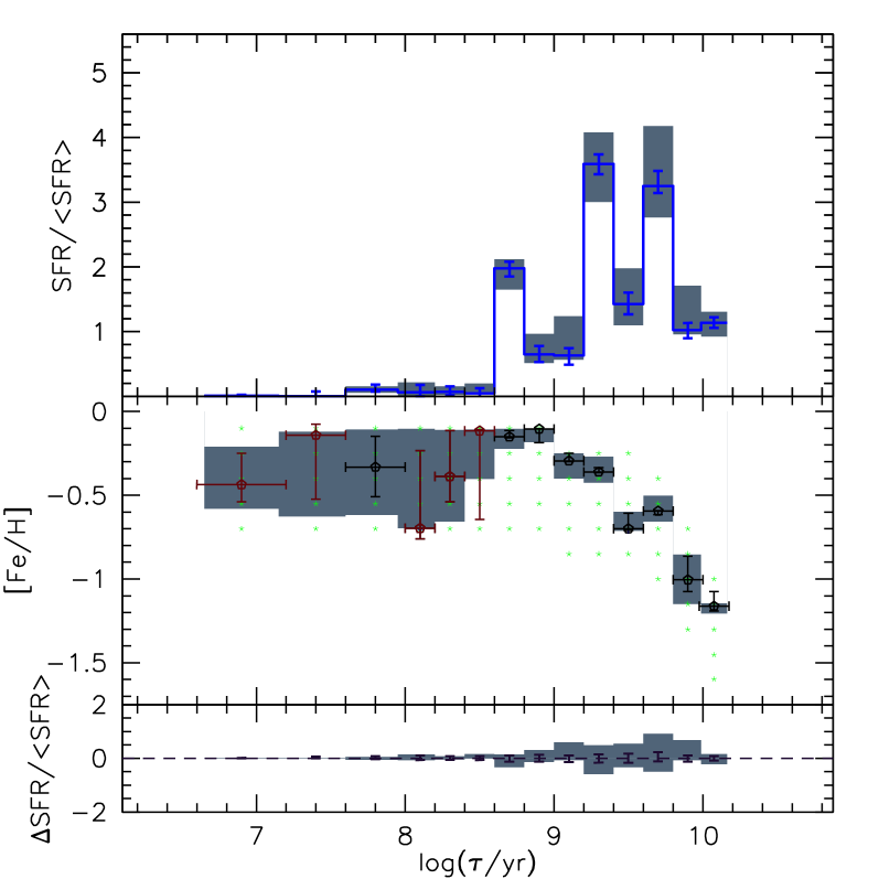
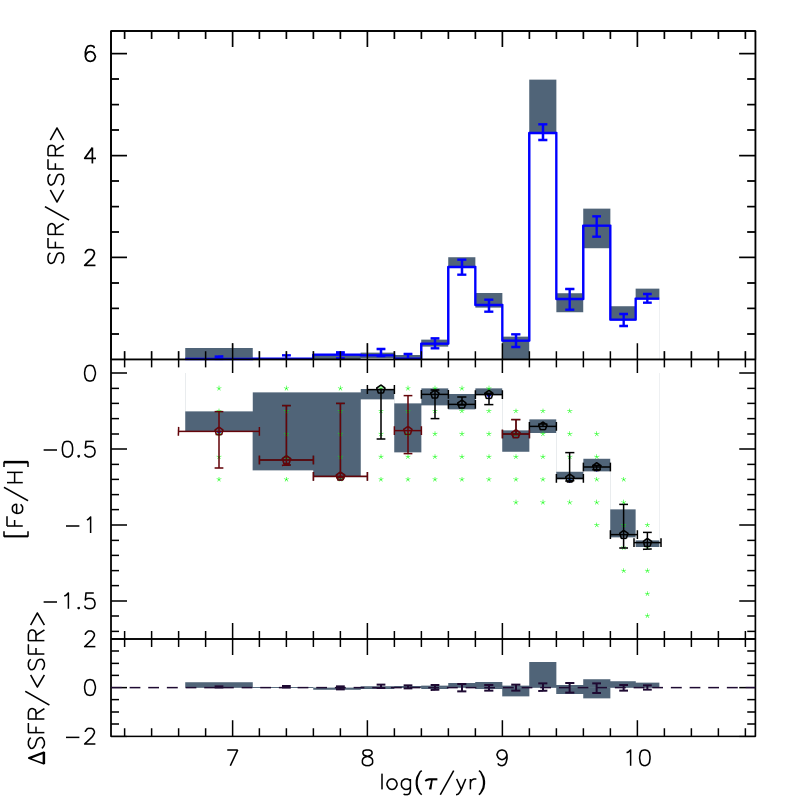
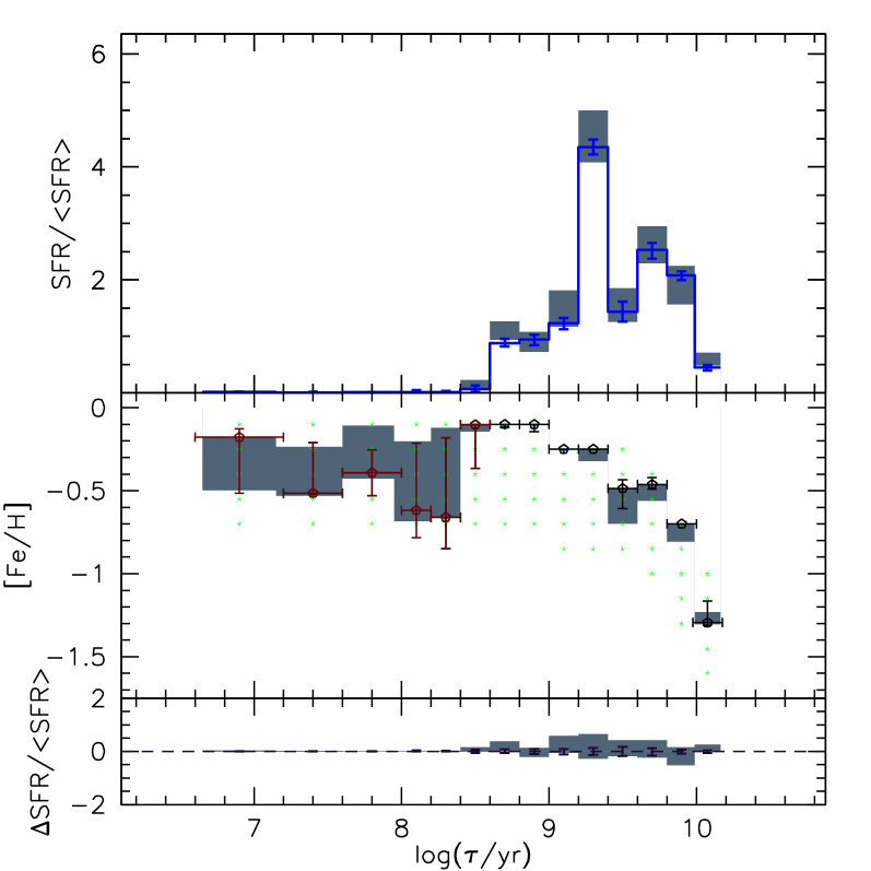
(c) ${\rm SFR}(t)$ and AMR of subregions G2, G6 and G10

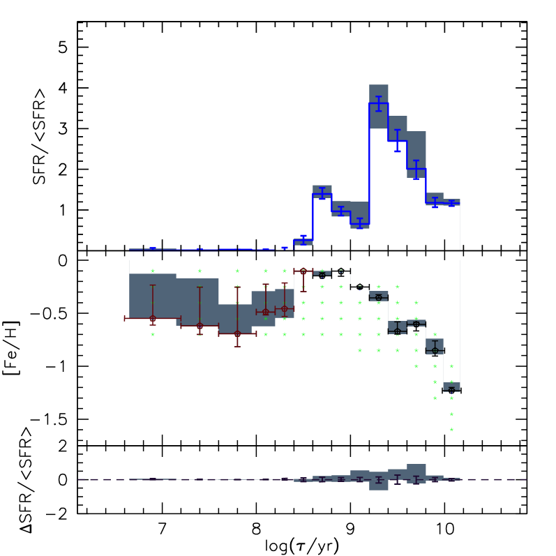
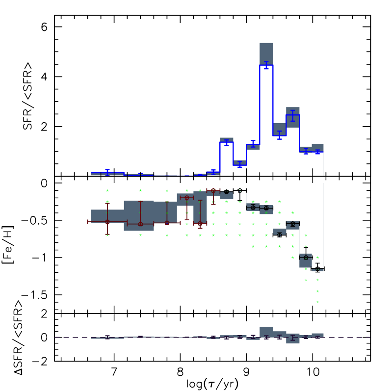
(d) ${\rm SFR}(t)$ and AMR of subregions G1 and G5

Figure 20: Same as in Fig. 18, but for the SFH for the 4_3 tile. The top left panels represent subregions closer to the LMC centre.

This tile presents average $A_{V}$ and $(m\!-\!M)_{0}$ values close to $\sim\!0.33$ and $\sim\!18.54$ mag, respectively. Fig. 16 shows the total ${\rm SFR}(t)$ and AMR. The SF of the young stellar population ($\mbox{$\log(t/{\rm yr})$}<8$) is as weak as in the 8_8 tile, whereas the SF in the older stellar population appears similar in most subregions (see Fig. 20). In addition to the oldest period of star formation at $\mbox{$\log(t/{\rm yr})$}\!>\!10.0$ with $\mbox{\rm[{\rm Fe}/{\rm H}]}\!\sim\!-1.0$ dex, it is possible to deduce three main peaks in the ${\rm SFR}(t)$:

1. The first at $\mbox{$\log(t/{\rm yr})$}=9.7$ and with $\mbox{\rm[{\rm Fe}/{\rm H}]}\!\sim\!-0.62$ dex, forming 31 % of the stellar mass in the tile.

2. The second at $\mbox{$\log(t/{\rm yr})$}=9.3$ and with an average $\mbox{\rm[{\rm Fe}/{\rm H}]}\!\sim\!-0.35$ dex, forming 15 % of the stellar mass.

3. The youngest at $\mbox{$\log(t/{\rm yr})$}=8.7$ with average $\mbox{\rm[{\rm Fe}/{\rm H}]}\!\sim\!-0.18$ dex. Although this peak appears evident in the ${\rm SFR}(t)$ plot, it represents just a modest 1.5 % of the stellar mass.

Note that the young SFR, with $\mbox{$\log(t/{\rm yr})$}\la 9$, is concentrated in subregions G4 and G8 (see Fig. 20), which are those more centrally located over the LMC disk. Regarding the two oldest peaks in the ${\rm SFR}(t)$  they are very similar to those derived for the 8_3 tile, supporting a good degree of mixing among older stellar populations across the LMC disk (see also Harris & Zaritsky 1999, 2009; Cioni et al. 2000; Cioni 2009; Nikolaev & Weinberg 2000; Blum et al. 2006; Carrera et al. 2011).

The AMR is well evaluated for all ages $\mbox{$\log(t/{\rm yr})$}>7.6$, where the ${\rm SFR}(t)$ is non negligible.

5.6 Tile 6_6

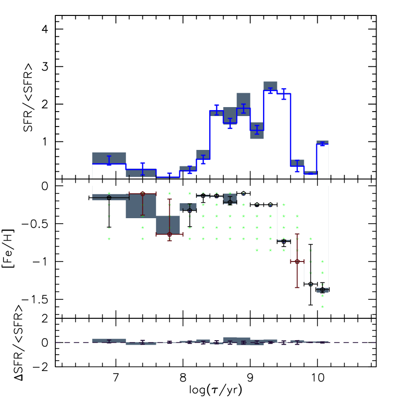
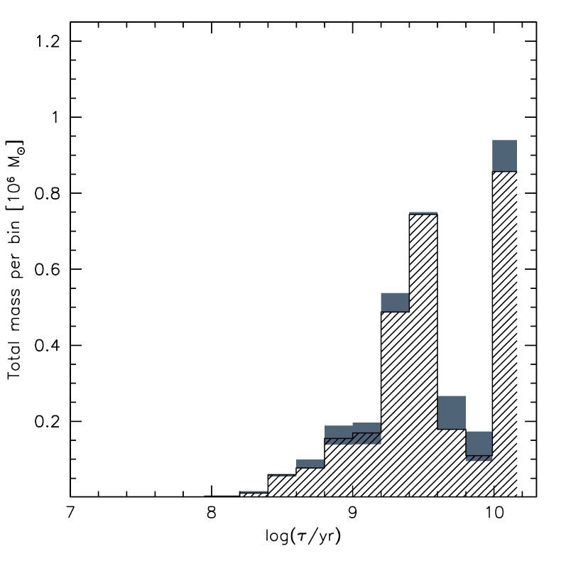
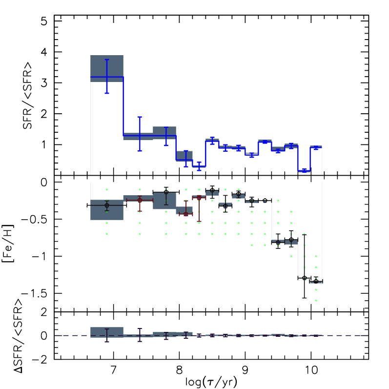
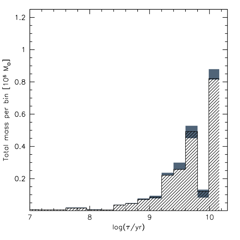
Figure 17: SFH results for subregions D1 (top panels) and D2 (bottom panels) in tile 6_6, assuming a fixed distance. The left panels must be compared to the left panels in Fig. 10, to illustrate the effect of fixing the distance. The right panels show the total mass formed per age bin.

In this tile we have recovered the SFH for the two small subregions D1 and D2, located on opposite sides of the tile and away from the 30 Doradus regions. Fig. 17 shows their SFHs as rederived after assuming a known distance. Since both regions are substantially different, their results have not been added as for the other tiles.

Subregion D1 is the most crowded and has some superposition with the LMC bar. Its best-fitting SFH solution presents a $\chi^{2}$ larger than those typically found in any other subregion analysed in this work, probably because of the larger photometric errors and/or higher differential extinction. Note also the larger $A_{V}$ values we find in both D1 and D2, with respect to other tiles: $\mbox{$A_{V}^{\rm TW}$}=0.65\;(-0.06,+0.03)$ mag for D1 and $\mbox{$A_{V}^{\rm TW}$}=0.60\pm 0.03$ mag for D2. For comparison, the $A_{V}$ values obtained by Zaritsky et al. (2004) in D1 and D2 are $\mbox{$A_{V}^{\rm CS}$}=0.50\pm 0.38$ mag (cool stars) and $\mbox{$A_{V}^{\rm HS}$}=0.68\pm 0.42$ mag (hot stars), $\mbox{$A_{V}^{\rm CS}$}=0.44\pm 0.34$ mag (cool stars) and $\mbox{$A_{V}^{\rm HS}$}=0.55\pm 0.39$ mag (hot stars), respectively, in good agreement with values derived here.

Despite the larger degree of crowding in this tile, the number of stars available in each subregion is very high and allows derivation of a very accurate SFH, as shown by the small error bars in Fig. 17, especially at the oldest ages. If we compare the ${\rm SFR}(t)$ of the two subregions for ages older than $\mbox{$\log(t/{\rm yr})$}=8.0$ the results are similar, with the oldest SF peak at $\mbox{$\log(t/{\rm yr})$}=10.1$, an age gap at $\mbox{$\log(t/{\rm yr})$}=9.9$, and a remarkably continuous ${\rm SFR}(t)$ between $\mbox{$\log(t/{\rm yr})$}\simeq 9.7$ and $\mbox{$\log(t/{\rm yr})$}=8.4$. According to the right panels in Fig. 17, 64 and 53 % of the total mass has been formed in this latter age interval, for subregions D1 and D2 respectively. It is tempting to associate this prolonged period of SF with the formation of the LMC bar. The gap in the ${\rm SFR}(t)$ for ages $\mbox{$\log(t/{\rm yr})$}=9.9$ has already been noticed before, and is extensively commented on Harris & Zaritsky (2009) as a main period of quiescent SF between $\sim 5$ and $\sim 12$ Gyr ago. Previous results regarding this feature (including Olsen 1999; Holtzman et al. 1999; Smecker-Hane et al. 2002; Harris & Zaritsky 2009) were based on deep HST data covering very small regions of the LMC bar. It is remarkable, and very encouraging, that the same feature can now be detected in ground-based data.

The ${\rm SFR}(t)$ for ages younger than $\mbox{$\log(t/{\rm yr})$}=8.0$ is more intense in D2, which is the subregion closer to both the 30 Dor complex and to the LMC centre.

5.7 The Magellanic interaction history and SFH peaks

We here discuss the present observational results on the two oldest peaks in the ${\rm SFR}(t)$ of the LMC in the context of the past interaction history of the LMC with the SMC and the Galaxy. These peaks are remarkable in the ${\rm SFR}(t)$ plots of outer disk tiles (4_3, 8_3 and 8_8), and correspond to the formation of $\sim 15$ % to 30 % of the total stellar mass each. A previous numerical model on chemical and dynamical evolution of the LMC showed that the star formation history of the LMC strongly depends on the LMC–SMC–Galaxy interaction history (e.g., Bekki & Chiba 2005). The model showed that the LMC–SMC tidal interaction for the last few Gyr can significantly enhance the SF in the LMC owing to the stronger tidal interaction between the LMC and the SMC (see their Fig. 9). The observed second peak at $\mbox{$\log(t/{\rm yr})$}=9.3$ ($\sim 2$ Gyr ago) can therefore correspond to the epoch when the mutual distance between the LMC and the SMC becomes significantly smaller so as to interact rather violently. The model also showed that the SFR of the LMC has peaks at 5.5 Gyr and 6.5 Gyr ago, which correspond to the epochs when the LMC strongly interacted with the Galaxy. Therefore, the observed first peak in the SFR at $\mbox{$\log(t/{\rm yr})$}=9.7$ ($\sim 5$ Gyr ago) might well correspond to the epoch when the LMC started its strong tidal interaction with the Galaxy. Given that there is no SFR peak for $\mbox{$\log(t/{\rm yr})$}>9.7$, it would be possible that the first SFR peak can contain fossil information as to when the LMC was accreted onto the Galaxy and commenced its tidal interaction with the Galaxy.

Some regions in tiles 4_3 and 8_3 show significant ${\rm SFR}(t)$ peaks at $\mbox{$\log(t/{\rm yr})$}=8.0\sim 8.2$, which however represent the formation of just a tiny fraction of their total stellar mass ($\sim 0.25$ % in 4_3 and 1.6 % in 8_3; see Figs. 16 and 15). It is possible that these episodes of enhanced ${\rm SFR}(t)$ are triggered by the last strong LMC–SMC interaction, which occurred roughly at this epoch according to previous numerical simulations (e.g., Gardiner & Noguchi 1996). The present study has also revealed that [Fe/H] appears to decrease after $\mbox{$\log(t/{\rm yr})$}\sim 8.1$ (see also van Loon et al. 2005) in spite of enhanced SFRs in some regions (e.g., tile $6\_6$). This result is intriguing, because canonical closed-box chemical evolution models predict increase in [Fe/H] of stars with time. If the observed apparent decrease in [Fe/H] is real (e.g., $\Delta\mbox{\rm[{\rm Fe}/{\rm H}]}\sim 0.2$ between $\mbox{$\log(t/{\rm yr})$}=8.2$ and $\mbox{$\log(t/{\rm yr})$}=7.0$ in the tile $6\_6$), then this means the following two possibilities. One is that the metal-poor gas, initially in the outer part of the LMC, was transferred to the inner regions to be converted into stars more metal-poor than the existing ones; the other is that the metal-poor gas was accreted by the LMC from outside (e.g., the Galactic Halo or the SMC) and then converted into metal-poor stars.

A number of observations showed that stellar populations in the LMC have a shallow radial metallicity gradient. For the $\sim 0.047$ dex kpc^-1 gradient derived from AGB stars (Cioni 2009, but see also Feast et al. 2010), two different regions with a difference in radial distances of $\sim 4$ kpc can have $\Delta\mbox{\rm[{\rm Fe}/{\rm H}]}\sim 0.2$ dex. Therefore it is not unlikely that star formation from gas initially in the outer part of the LMC can be responsible for the decrease in [Fe/H] in the AMR for some regions of the LMC. The second possibility ( metal-poor gas being accreted from outside the LMC), which is more intriguing than the first, is strongly supported by a previous dynamical model that showed gas-transfer between the LMC and the SMC $\sim 0.2$ Gyr ago (Bekki & Chiba 2007). The model clearly showed that the outer part of the SMC’s gas disk can be stripped by the LMC–SMC tidal interaction and finally be accreted efficiently onto the LMC. Given that the SMC has a metallicity that is significantly smaller than that of the LMC, new stars formed from gas transferred from the SMC inevitably have smaller metallicities and thus explain the observed young and metal-poor stars in the LMC.

Recently Olsen et al. (2011) found that about 5% of the LMC AGB stars have line-of-sight velocities that appear to oppose the sense of rotation of the LMC disk. They have also found an association of the kinematically distinct population with the peculiar gaseous arm in the LMC and accordingly claimed that the stars and the peculiar arm can originate from the SMC. These accreted SMC populations in the LMC clearly support the second possibility. However, it is still unclear how much of the SMC gas needs to be accreted onto the LMC so as to quantitatively explain the observed metallicities of young metal-poor stars in the LMC. It is doubtlessly worthwhile for future theoretical studies to investigate this issue by using sophisticated chemodynamical simulations of the LMC and the SMC for the most recent 0.2 Gyr.

So far we have considered only a scenario in which the LMC and the SMC have had bound orbits around the Galaxy for the last $\sim 6$ Gyr. It is however observationally unclear whether these bound orbits are consistent with recent proper motion results of the MCs. Recent HST proper motion studies of the LMC (e.g., Kallivayalil et al. 2006) have shown that the LMC has a high velocity ($\sim 380$ km s^-1), which suggests that the LMC passed by the Galaxy for the first time about 0.2 Gyr ago (e.g., Besla et al. 2007). On the other hand, the latest ground-based observational studies of the proper motions of the MCs have shown that the LMC has a lower velocity (300–340 km s^-1; e.g. Costa et al. 2009; Vieira et al. 2010). Recent numerical simulations of the past orbit of the LMC (and the SMC) demonstrated that the LMC is bound to the Galaxy for at least $\sim 5$ Gyr if the LMC’s velocity is less than 360 km s^-1 (Bekki 2011). The observational results by Kallivayalil et al. (2006) and Vieira et al. (2010) are around this limit and are barely consistent with each other, implying that more observational data sets are required to provide strong constraints on the orbital history of the LMC.

5.8 Concluding remarks

This work demonstrates that SFH-recovery in VMC data works as well as expected (Kerber et al. 2009), and produces sensible results for the values of distance and reddening in every $\sim\!0.12$ deg² subregion analysed. Moreover, we show that we can take advantage of the correlation between the parameters of different subregions – in our case, the distances – to improve the SFH results, notably reducing the final error bars. It is obvious that the same techniques can be further improved by taking advantage of other correlations – e.g., of the smoothness of the old SFH over large scales, which is also evident in this work.

These aspects will be fully explored as more data from the survey is considered. We note that the present results refer to just a small subset of the VMC: four tiles covering less than 5.6 deg², with some subregions deliberately left out of the analysis because of either problems with the photometry (in VIRCAM detector 16 of each tile), or of the large and variable extinction (as for most of the 30 Dor region). The VMC $K_{\rm s}$-band imaging has been 100 % completed in only one of these tiles. The final survey area as planned will include 116 deg² covering the entire LMC, and additional 45 deg² over the SMC, 20 deg² over the Bridge, and a small subset (3 deg²) of the Stream. The perspectives for deriving detailed and reliable spatially resolved SFHs all across the Magellanic system, seem very promising.

Appendix A SFH results for each subregion

For the sake of completeness, this appendix presents the SFH results for all subregions of all tiles. All SFH data, including tables and figures, are available on the VMC main site, http://star.herts.ac.uk/ mcioni/vmc/, and are regularly updated as the survey and analysis proceed.