A gap in the spectrum of the Neumann-Laplacian on a periodic waveguide

Abstract

Abstract

We will study the spectral problem related to the Laplace operator in a singularly perturbed periodic waveguide. The waveguide is a quasi-cylinder with contains periodic arrangement of inclusions. On the boundary of the waveguide we consider both Neumann and Dirichlet conditions. We will prove that provided the diameter of the inclusion is small enough in the spectrum of Laplacian opens spectral gaps, i.e. frequencies that does not propagate through the waveguide. The existence of the band gaps will verified using the asymptotic analysis of elliptic operators.

35P05; 34E05; 34E10; 76M45

1 Introduction

The main goal in this paper is to study the spectral properties of the Neumann-Laplacian on the periodic singularly perturbed periodic quasi-cylinder $\Omega(\epsilon)$:

$$-\Delta u^{\epsilon}(x) = \lambda^{\epsilon}u^{\epsilon}(x),\ x\in\Omega(\epsilon),$$ (1)

$$\partial_{n}u^{\epsilon}(x) = 0,\ x\in\partial\Omega(\epsilon).$$ (2)

This spectral problem should be interpreted as a singular perturbation of the same problem in the straight cylinder $\Omega=\omega\times{\mathbb{R}}\subset{\mathbb{R}}^{3}$.

The quasi-cylinder $\Omega(\epsilon)$ is a periodic set which depends on a small parameter $\epsilon>0$. It is obtained from the straight cylinder $\Omega$ by a periodic nucleation of small voids with diameter of order $\epsilon$ (see fig. 1a and fig 1b, respectively). We remark that without lost of generality we have reduced the period to one by rescaling.

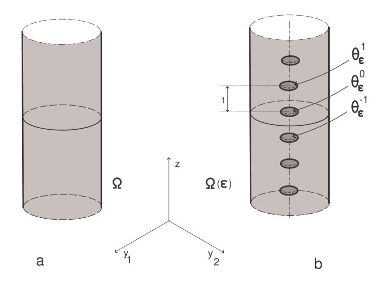
Figure 1: A cylinder and a quasi-cylinder with periodic family of voids

It is known (e.g. [28]) that the spectrum $\sigma$ of the Neumann-Laplacian in the straight cylinder $\Omega$ implies the continuous spectrum $\sigma_{c}$ which is the closed positive real semi-axis $\overline{\mathbb{R}_{+}}$, and the point spectrum is empty. In particular, for any real $\mu>0$ the functions, or oscillating waves,

$$e^{\pm i\sqrt{\mu}z},$$ (3)

give rise to a singular Weyl sequence of the problem operator $A$ at the point $\mu\in\overline{\mathbb{R}_{+}}$ (cf. §9.1 in [1]).

The structure of the spectrum $\sigma(\epsilon)$ in the perturbed quasi-cylinder $\Omega(\epsilon)$ is much more complicated. Owing to the Gel’fand transform [10] (see Section 2) and the Floquet-Bloch theory (see e.g. [13, 21]) the spectrum $\sigma(\epsilon)$ of the Neumann-Laplacian is endowed with the band-gap structure. Namely, the essential spectrum $\sigma(\epsilon)=\sigma_{e}(\epsilon)$ is a union of closed connected segments $\Upsilon_{n}(\epsilon)\subset\overline{\mathbb{R}_{+}}$:

$$\sigma(\epsilon)=\bigcup_{n\in\mathbb{N}}\Upsilon_{n}(\epsilon).$$

We obtain a spectral gap in the spectrum if there exist an interval in the positive real semi-axis which is free of the spectrum, see the left part of fig. 2. However, when the segments overlap each other (see the right part of fig.2), no spectral gap opens.

Here we note that the essential spectrum $\sigma_{e}(\epsilon)$ coincides with the continuous spectrum provided none of the segments $\Upsilon_{n}(\epsilon)$ collapses to a single point, which becomes an eigenvalue of the operator $A(\epsilon)$ with infinite multiplicity, and belongs to the point spectrum while the discrete spectrum is still empty. A negative answer to this possibility is still an open question and the authors can only prove the following: For any $t>0$ there exists $\epsilon_{t}>0$ such that $\sigma_{p}(\epsilon)\cap[0,t]=\emptyset$ when $\epsilon\in(0,\epsilon_{t}]$. We do not pay any attention to this incomplete result and therefore always speak in this paper about the essential spectrum.

Figure 2: The gap between the first and second bands, while a gap between the second and the fourth band is covered by the third one

In the literature the existence of spectral gaps is mainly investigated for periodic media which are infinite in all directions while the coefficients of differential operators, both in scalar and matrix case, are usually assumed to be contrasting (see e.g. [5, 6, 9, 11, 30] for scalar problems and [4, 19] for systems). Much less results are obtained for periodic waveguides, which are infinite in one direction only. In this case spectral gaps ought to be opened by varying the shape of the periodicity cell only which is in accordance with the results in the known engineering practise.

There are two useful approaches to fulfil the goal. The first one utilises the asymptotic analysis of the spectrum for the associated model problem in the periodicity cell, like we do in the present paper. This approach has been realised for the Dirichlet-Laplacian in papers [29, 7, 20, 2] and others. We emphasise that our results for the Neumann-Laplacian are completely new and require different techniques.

The second approach is based on the application of sharp parameter-dependent estimates provided by Korn’s inequalities, usually weighted and anisotropic, see e.g. [22, 17, 18] and others. On one hand, this approach does not require a precise description of the dependence of the cell shape perturbation on the small geometric parameter, but, in contrast to the first approach, one can only prove the existence of one or several spectral gaps without any information on the position and width of the gaps.

Combining of the above-mentioned approaches one could get much more elaborated results by using their advantages. However, we cannot examine here the whole spectrum and to our knowledge there does not exist any results of this type. Here indeed we discuss only the first spectral gap.

To prove or to disprove the existence of a gap between the segments $\Upsilon_{1}(\epsilon)$ and $\Upsilon_{2}(\epsilon)$ (cf. fig. 2), we employ the method of compound asymptotic expansions [14] to the associated model spectral problems in the periodicity cell

$$\varpi_{\epsilon}=\varpi\setminus\overline{\theta_{\epsilon}^{0}},\quad\varpi=\omega\times(0,1)$$ (4)

of the quasi-cylinder (5). The straight cylinder with the small void $\theta^{0}_{\epsilon}$ (see the two-dimensional dummy in fig. 3b) is nothing but a good example of a domain with the singularly perturbed boundary $\partial\varpi_{\epsilon}=\partial\varpi\cup\partial\theta_{\epsilon}^{0}$. The asymptotic analysis of the eigenvalues for the Laplace operator have been developed at a great extend in [15, 25, 8, 16, 12, 23, 24] and many others. However, the dependence of the model problem on the dual variable $\eta\in[0,2\pi)$ of the Gel’fand transform brings a serious complication to both, the formal asymptotic procedures and the justification since, instead of a single spectral problem, we have to deal with a family of spectral problems dependent on the real parameter $\eta\in[0,2\pi)$ (see Section 3 and Section 4 for more details).

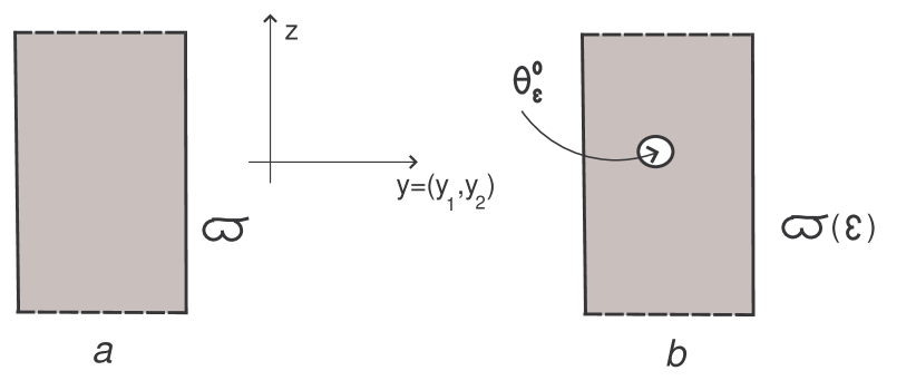
Figure 3: The two-dimensional dummy of the periodicity cell

2 Preliminaries and notations

2.1 The quasi-cylinder and the Gel’fand transform

The purpose of this section is to explain what do we mean by a periodic quasi-cylinder. There are several ways to describe it; but here we start with the straight cylinder which is the cartesian product of a bounded Lipschitz domain $\omega\subset\mathbb{R}^{2}$ and the real line: $\Omega=\omega\times\mathbb{R}$.

Consider now a fixed bounded smooth domain $\theta$ with the coordinate origin $\xi=0$ in its interior. We introduce the family of sets $\theta^{j}_{\epsilon}$ by defining

$$\theta^{j}_{\epsilon}=\{x=(y_{1},y_{2},z):\ (y_{1},y_{2},z-j)\in\theta^{0}_{\epsilon}\},\theta^{0}_{\epsilon}=\{x:\xi=\epsilon^{-1}(x-x^{0})\in\theta\},$$

where $x^{0}\in\varpi=\omega\times(0,1)$. Note that the diameter of the set $\theta^{j}_{\epsilon}$ is of order $\epsilon$.

The quasi-cylinder $\Omega(\epsilon)$ is a periodic set which depends on a small parameter $\epsilon>0$ and it will be obtained from the straight cylinder $\Omega$ excluding the sets $\overline{\theta^{j}_{\epsilon}}$ from it (see fig. 1a and fig 1b, respectively). In other words, the quasi-cylinder can be written as

$$\Omega(\epsilon)=\Omega\setminus\bigcup_{j\in\mathbb{Z}}\overline{\theta^{j}_{\epsilon}}.$$ (5)

We call the set $\varpi(\epsilon)=\varpi\setminus\theta^{0}_{\epsilon}$ in (4) as the periodicity cell of the quasi-cylinder. Note that the cylinder $\Omega$ can be viewed as a quasi-cylinder with the straight periodicity cell $\varpi$ as in (4).

We recall here the definition of the Gel’fand transform [10]:

$$v(y,z)\mapsto\,V(y,z,\eta)=\frac{1}{\sqrt{2\pi}}\sum_{j\in\mathbb{Z}}e^{-i\eta j}v(y,z+j),$$ (6)

where $(y,z)\in\Omega(\epsilon)$ on the left, $\eta\in[0,2\pi)$ and $(y,z)\in\varpi(\epsilon)$ on the right. As it is well known this operator is an isometric isomorphism from $L^{2}(\Omega(\epsilon))$ onto $L^{2}(0,2\pi;L^{2}(\varpi(\epsilon)))$ and an isomorphism between the Sobolev spaces $H^{1}(\Omega(\epsilon))$ and $L^{2}(0,2\pi;H^{1}_{\eta}(\varpi(\epsilon)))$ (see e.g. [21, 13]). Here $L^{2}(0,2\pi;L^{2}(\varpi(\epsilon)))$ consists of $L^{2}(\varpi(\epsilon))$-valued (complex) $L^{2}$-functions on $[0,2\pi]$. Similarly, the space $L^{2}(0,2\pi;H^{1}_{\eta}(\varpi(\epsilon)))$ contains those $H^{1}_{\eta}(\omega(\epsilon))$-valued (complex) $L^{2}$-functions on $[0,2\pi]$. Finally we have denoted by $H^{1}_{\eta}(\varpi(\epsilon))$ the space of Sobolev functions $f$ which are quasi-periodic in the $z$-variable, i.e. such that function $(y,z)\mapsto e^{-i\eta z}f(y,z)$ is 1-periodic in $z$.

2.2 The relationship between waves and Floquet waves in the straight cylinder

Before going into the asymptotic analysis of the spectral problem in the periodic quasi-cylinder we will study the relationship of the standard wave solutions and Floquet waves for the Neumann-Laplacian in the cylinder $\Omega$. They are the solutions of the differential equation

$$-\Delta_{x}u(x)=\lambda u(x),\ x\in\Omega\,,$$ (7)

supplied with the Neumann conditions on the boundary

$$\partial_{n}u(x)=0,\ x\in\partial\Omega\,.$$ (8)

Applying the Gel’fand transform to (7) and (8) we obtain the model problem in the periodicity cell $\varpi$ with the dual Gel’fand parameter $\eta\in[0,2\pi)$, namely, the differential equation

$$-\Delta_{x}U(x,\eta)=\Lambda(\eta)U(x,\eta),\ (y,z)\in\varpi,$$ (9)

the Neumann condition on the lateral boundary of $\gamma=\partial\varpi$

$$\partial_{n}U(x;\eta)=0,\ x\in\gamma,$$ (10)

and the quasi-periodicity conditions on the opposite ends of the cylindrical cell $\varpi=\omega\times(0,1)$:

$$U(y,0)=e^{-i\eta}U(y,1),\ \partial_{z}U(y,0)=e^{-i\eta}\partial_{z}U(y,1),\ y\in\omega.$$ (11)

Let $\Lambda_{p}$ be an eigenvalue and let $U_{p}$ be the corresponding eigenfunction of the model spectral problem (8)-(11), then the Floquet wave can be written as

$$\Omega\ni(y,z)\mapsto e^{i\eta[z]}U_{p}(y,z-[z])$$ (12)

where $[z]\in\mathbb{Z}$ stands for the entire part of the real number $z$. Notice that function (12) is smooth due to the quasi-periodicity conditions (11) and it becomes a solution of the homogeneous problem (7) with the spectral parameter $\lambda=\Lambda_{p}$.

Any function of the type (12) must be obtained from the standard waves

$$(y,z)\mapsto e^{i\zeta z}V_{q}(y)$$ (13)

in the cylinder $\Omega$, where $\zeta\in\mathbb{R}$ is the dual Fourier variable and $V_{q}$ is an eigenfunction of the model problem

$$-\Delta_{y}V(y)=MV(y),\quad y\in\omega\,,\quad\partial_{n}V(y)=0,y\in\partial\omega$$ (14)

on the cross-section $\omega$. Notice that the wave solution (13) with $q=1$ and $V_{1}(y)=const$ corresponds to the eigenvalue $M_{1}=0$ and coincides with the wave solution (3) where

$$\mu=\zeta^{2}$$

stands for the parameter in the Helmholtz operator $\Delta_{x}+\mu$. The main difference between formulae (12) and (13) follows from the role played by the parameters $\eta\in[0,2\pi)$ and $\zeta\in\mathbb{R}$.

We write the wave solution (13) as follows:

$$e^{i\zeta z}V_{q}(y)=e^{i(\zeta-2\pi m)[z]}e^{i(\zeta-2\pi m)(z-[z])}e^{2\pi miz}V_{q}(y)$$ (15)

where $m=[(2\pi)^{-1}\zeta]$ is the maximal integer such that $2\pi m\leq\zeta$. Now we denote the first multiplier on the right of (15) by $e^{i\eta[z]}$ and the remaining part by $U_{p}(y,z-[z])$ so that

$$U_{p}(y,z) = e^{i\eta z}e^{2\pi miz}V_{q}(y),$$ (16)

$$\eta = \zeta-2\pi m\in[0,2\pi).$$

Since $e^{2\pi miz}$ is 1-periodic in $z$, we see that the function $U_{p}$ satisfies the quasi-periodicity conditions (11). In other words, (15) implies the Floquet representation (12) of the wave solution (13) with the ingredients (16).

Relationship (16) helps us to list all eigenpairs $\{\Lambda_{p},U_{p}\}$ of the model problem in the straight cell $\varpi$ in terms of the eigenvalues

$$0=M_{1}<M_{2}\leq M_{3}\leq\ldots$$ (17)

and eigenfunctions $\{V_{1},\,V_{2},\,V_{3},\dots\}$ of the model problem (14). Namely, there holds the relations

$$\Lambda_{q,m}(\eta)=M_{q}+(\eta+2\pi m)^{2},\quad q\in{\mathbb{N}},\,m\in\mathbb{Z}.$$ (18)

We emphasise that the eigenvalues $\Lambda_{q,m}(\eta)$ are now enumerated with two indexes so that it is necessary to reorder them to get the monotone increasing unbounded sequence

$$\Lambda_{1}(\eta)\leq\Lambda_{2}(\eta)\leq\cdots\leq\Lambda_{k}(\eta)\leq\cdots.$$ (19)

The lowest dispersion curve (18) in fig. 4a, corresponding to the smallest eigenvalue $M_{1}=0$ of the Neumann problem in $\omega$, divides into an infinite family of smooth finite curves which by above formulae are joined to the lattice in fig 4b. In the sequel we are mainly interested in the couple of lowest curves in the lattice which are redrawn in fig 5.a,

$$\Lambda^{0}_{+}(\eta):=\Lambda_{0,0}(\eta)=\eta^{2},\ \Lambda^{0}_{-}(\eta):=\Lambda_{0,-1}(\eta)=(\eta-2\pi)^{2}.$$ (20)

We shall use the notation (20) throughout the paper.

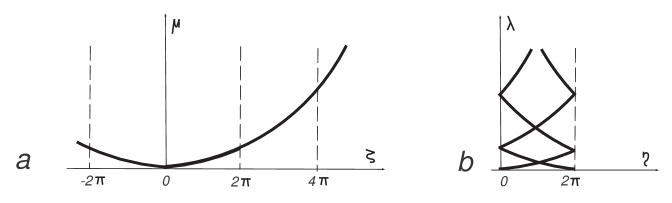
Figure 4: The lowest dispersion curve and the lattice frame made from it

The variational formulation of problem (9)-(11) reads as

$$(\nabla_{x}U,\nabla_{x}V)_{\varpi}=\Lambda(\eta)(U,V)_{\varpi}\,,V\in H^{1}_{\eta}(\varpi)\,.$$ (21)

Since for any real parameter $\eta$ the bilinear form on the left-hand side of (21) is symmetric, closed and positive, we can associate with it a self-adjoint positive operator in the Lebesque space $L^{2}(\varpi)$ [1, Thm. 10.1.2]. Moreover, the compact embedding $H^{1}(\varpi)\subset L^{2}(\varpi)$ and Theorems 10.1.5 and 10.2.2 in [1] ensure that indeed the spectrum of this operator is discrete and forms an unbounded non-negative sequence (19) which is constructed from (17).

2.3 Perturbation of the dispersion curves

In the perturbed periodicity cell $\varpi_{\epsilon}$ the both dispersion curves (20) experience a perturbation and, in principle, there can occur two different situations pictured in fig. 5.b. and 5.c. First, the dispersion curves $[0,2\pi)\ni\eta\to\Lambda_{\pm}^{\epsilon}(\eta)$ may still intersect so that the spectral segments $\Upsilon_{1}(\epsilon)$ and $\Upsilon_{2}(\epsilon)$ touch each other and the gap between them is closed. The second possibility is that the graphs of the functions

$$\eta\mapsto\Lambda^{\epsilon}_{1}(\eta),\,\eta\mapsto\Lambda^{\epsilon}_{2}(\eta)$$

do not intersect and the area overshadowed in fig. 5c projects into a gap between segments $\Upsilon_{1}(\epsilon)$ and $\Upsilon_{2}(\epsilon)$. In the sequel we will describe when the gap appears and indicate asymptotically its position and width.

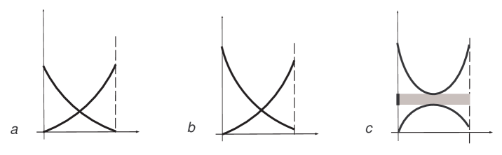
Figure 5: Unperturbed (a), intersecting (b) and disjoint (c) curves

Before proceeding with the problem statement, the formal asymptotic analysis and the justification, we note that the gap opens only under the condition

$$M_{1}+\pi^{2}<M_{2}.$$ (22)

Otherwise, the segment $\Upsilon_{2}(\epsilon)$, which corresponds to the perturbed eigenvalues in (18) with $q=2$ and $m=0,-1$ covers the gap opened between the segments $\Upsilon_{1}(\epsilon)$ and $\Upsilon_{3}(\epsilon)$ (see fig.6) which are now generated by eigenvalues in (18) with $q=1$ and $m=0,-1$.

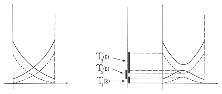
Figure 6: Overlapping bands. The dotted lines correspond to the perturbation of the lowest curves in fig. 5.a.

However, the rescaling performed in the very beginning rescales also eigenvalues. To see this, assume that the period $l$ of the void nucleation is bigger than one. Now the rescaling diminishes the size of the cross-section, i.e. the change of the variables $(y,z)\to(y^{\prime},z^{\prime})=(l^{-1}y,l^{-1}z)$ yields the shrunken cross-section

$$\omega^{\prime}=\{y^{\prime}\in\mathbb{R}^{2}:\ ly^{\prime}\in\omega\}.$$

Simultaneously, eigenvalues of the model problem in $\omega$ changes into the eigenvalues $M_{1}^{\prime}=0$ and $M_{2}^{\prime}=l^{2}M_{2}$ of the model problem in the shrunken cross-section $\omega^{\prime}$. By choosing $l$ large enough we fulfil the condition (22) for $M_{1}^{\prime}$. In other words, posing the small voids $\theta_{\epsilon}^{0}$ with a sufficiently large period may open a gap in the essential spectrum, where as if the period of the voids is sufficiently small first triple of the spectral bands surely overlap.

Assuming condition (22) we study the spectral problem (1)-(2). Applying the Gel’fand transform (6) to problem (1)-(2), we obtain the model spectral problem in the periodicity cell $\varpi_{\epsilon}$ depending on $\eta\in[0,2\pi)$:

$$-\Delta U^{\epsilon}(y,z) = \Lambda^{\epsilon}(\eta)U^{\epsilon}(y,z),\ (y,z)\in\varpi_{\epsilon}\,,$$ (23)

$$\partial_{n}U^{\epsilon}(x) = 0,\ x\in\gamma\cup\partial\theta(\epsilon)\,,$$ (24)

$$U^{\epsilon}(y,0)=e^{-i\eta}U^{\epsilon}(y,1), \partial_{z}U^{\epsilon}(y,0)=e^{-i\eta}\partial_{z}U^{\epsilon}(y,1),\ y\in\gamma_{0}.$$ (25)

As above, using Theorem 10.1.2 [1] we associate with these spectral problems a family of unbounded positive self-adjoint operators $T^{\epsilon}(\eta)$ on $L^{2}(\varpi_{\epsilon})$ with discrete spectra, i.e., the eigenvalue sequences

$$0\leq\Lambda^{\epsilon}_{1}(\eta)\leq\Lambda^{\epsilon}_{2}(\eta)\leq\cdots\leq\Lambda^{\epsilon}_{k}(\eta)\leq\cdots\rightarrow\infty.$$

The immediate objective becomes to construct asymptotics for these eigenvalues as $\epsilon\to+0$.

2.4 Mixed boundary value problem

Although all the calculations are presented for the Neumann conditions on the boundary of the quasi-cylinder $\Omega(\epsilon)$, we also discuss slight modifications, which are needed to adapt our calculations to the mixed boundary value problem

$$-\Delta u^{\epsilon}(x) = \lambda^{\epsilon}u^{\epsilon}(x),\ x\in\Omega(\epsilon)\,,$$

$$\partial_{n}u^{\epsilon}(x) = 0,\ x\in\partial\Omega(\epsilon)\setminus\partial\Omega=\cup_{j\in\mathbb{Z}}\partial\theta^{j}_{\epsilon}\,,$$ (26)

$$u^{\epsilon}(x) = 0,x\in\partial\Omega\,.$$

We emphasise that the asymptotic procedure of [14] employed here is not sensitive to the type of boundary conditions on the lateral part of the boundary $\partial\omega\times(0,1)$ of the periodicity cell is employed. However, the change of the boundary condition from Neumann to Dirichlet on the surfaces of small voids crucially simplifies the asymptotic analysis. In this way our paper becomes much more technical than [20] and [2], where the Dirichlet problem was considered in the regularly and singularly perturbed periodicity cells. The particular conclusions on the geometrical characteristics of the gap are also different.

3 The formal asymptotic procedure

In this section we present a calculation which furnishes an asymptotic formula for the first two eigenvalues (20). In order to simplify the presentation we start with considering the case when the eigenvalues for the model problem are simple, e.g. when the Gel’fand dual variable $\eta$ is not equal to $\pi$. Notice that the dispersion curves in fig. 5a intersect each other just at $\eta=\pi$, and we examine this situation in the end of this section.

In Sections 3.3 and 3.4 we give detailed calculations of the boundary layers and a regular terms which lead to a direct formula for the main correction term in the asymptotics of the eigenvalues. With this asymptotic formula we are then able to consider also the case $\eta\approx\pi$ although at $\eta=\pi$ where the model problem has a multiple eigenvalue. As a result, in Section 3.5 we derive a system of two linear algebraic equations from which we can find out the perturbation terms in the asymptotics of the eigenvalues when $\eta$ approximately equal to $\pi$.

To make the necessary conclusion for the case $\eta\approx\pi$, we will apply the trick proposed in [20] and introduce the additional deviation parameter $\psi$ in the representation

$$\eta=\pi+\psi\epsilon^{3}\,.$$ (27)

With the help of this new variable $\psi\in[-\psi_{0},\psi_{0}]$ we can write the asymptotic formulae at the $c\epsilon^{3}$-neighbourhood of the point $\eta=\pi$.

We emphasise here the following difference in the notation: In Sections (3.1)-(3.4) we set

$$\Lambda_{+}^{\epsilon}(\eta) = \Lambda_{1}^{\epsilon}(\eta),\,\Lambda_{-}^{\epsilon}(\eta)=\Lambda_{2}^{\epsilon}(\eta),\,\eta\in[0,\pi),$$ (28)

$$\Lambda_{+}^{\epsilon}(\eta) = \Lambda_{2}^{\epsilon}(\eta),\,\Lambda_{-}^{\epsilon}(\eta)=\Lambda_{1}^{\epsilon}(\eta),\,\eta\in(\pi,2\pi),$$

while in Section (3.5)

$$\Lambda_{+}^{\epsilon}(\eta)=\Lambda_{2}^{\epsilon}(\eta),\,\Lambda_{-}^{\epsilon}(\eta)=\Lambda_{1}^{\epsilon}(\eta),\,\eta=\pi.$$ (29)

The evident difference in the notations (28) and (29) helps to keep similar asymptotic formulae in both cases.

Calculations in Sections 3.1-3.4 are given for the Neumann problem (1)-(2) in such a way that they can easily adopted for the mixed boundary value problem (2.4). Namely, the eigenpair of the problem (14) $\{M_{1}=0$, $V_{1}=const\}$ must be replaced by the first eigenpair $\{M_{1},V_{1}\}$ of the Dirichlet problem

$$-\Delta_{y}V(y)=MV(y),\,y\in\omega,\qquad V(y)=0,\,y\in\partial\omega\,.$$ (30)

Notice that the eigenvalue $M_{1}$ is positive and simple while the corresponding eigenfunction $V_{1}$ can be chosen positive inside the cross-section $\omega$.

3.1 Asymptotic expansions

To describe the asymptotic behaviour of two first eigenvalues $\Lambda^{\epsilon}_{\pm}(\eta)$, we accept the following ansatz:

$$\Lambda^{\epsilon}_{\pm}(\eta)=\Lambda^{0}_{\pm}(\eta)+\epsilon^{3}\Lambda^{\prime}_{\pm}(\eta)+\widetilde{\Lambda}^{\epsilon}_{\pm}(\eta),$$ (31)

where $\Lambda^{0}_{\pm}(\eta)$ is the eigenvalue (20) of problem (7)-(9), $\Lambda^{\prime}_{\pm}(\eta)$ is a correction term and $\widetilde{\Lambda}^{\epsilon}_{\pm}(\eta)$ a small remainder to be evaluated and estimated.

According to general asymptotic method in domains with singular perturbations of the boundaries (see e.g. [14]) the corresponding asymptotic ansatz for eigenfunctions reads as follows

$$U^{\epsilon}_{\pm}(x;\eta) = U^{0}_{\pm}(x;\eta)+\epsilon\chi(x)W^{1}_{\pm}(\epsilon^{-1}(x-x^{0});\eta)$$ (32)

$$+ \epsilon^{2}\chi(x)W^{2}_{\pm}(\epsilon^{-1}(x-x^{0});\eta)+\epsilon^{3}U^{\prime}_{\pm}(x;\eta)+\widetilde{U}^{\epsilon}_{\pm}(x;\eta).$$

The functions $W^{j}_{\pm}$ are of boundary layer type and $\chi$ is a smooth cut-off function which equals one in a neighbourhood of the point $x^{0}$ and vanishes in the vicinity of the boundary $\partial\varpi$. The functions $U^{0}_{\pm}$ are the first two eigenfunctions of the unperturbed problem (cf. formula (16)), namely

$$U^{0}_{+}(x;\eta)=e^{i\eta z}V_{1}(y),\quad U^{0}_{-}(x;\eta)=e^{i(\eta-2\pi)z}V_{1}(y),$$ (33)

where $V_{1}$ is the first eigenfunction of the Laplace operator on the cross-section, normalised in $L^{2}(\varpi)$. Clearly, both the functions (33) meets the quasi-periodicity conditions (11). Note that in the case of the Neumann boundary conditions on $\partial\Omega$ the function $V_{1}$ is just a constant. One readily verifies that since $M_{1}=0$ is the first eigenvalue of the Laplacian on the cross-section in the Neumann case, the first couple of eigenvalues of the unperturbed problem take the form (20).

3.2 The boundary layers

The boundary layer $W^{1}_{\pm}$ depends on the “fast” variables (“stretched“ coordinates)

$$\xi=(\xi_{1},\xi_{2},\xi_{3})=\epsilon^{-1}(x-x^{0})$$

and is needed to compensate for that the main regular term $U^{0}_{\pm}$ in the expansion does not fulfil the Neumann type boundary condition

$$\partial_{n(x)}u(x)=0,\,x\in\partial\theta_{\epsilon}.$$

By the Taylor formula applied to the function $U^{0}_{\pm}$ in the ”slow“ variables $x$, we have

$$\partial_{n(\xi)}U^{0}_{\pm}(x;\eta)=n(\xi)\cdot\nabla_{x}U^{0}_{\pm}(x^{0})+O(\epsilon),\,x\in\partial\theta_{\epsilon}.$$

Thus $W^{1}_{\pm}$ ought to be a solution of the exterior Neumann problem

$$\Delta_{\xi}W^{1}_{\pm}(\xi) = 0,\ \xi\in\mathbb{R}^{3}\setminus\bar{\theta}\,,$$ (34)

$$\partial_{n(\xi)}W^{1}_{\pm}(\xi) := G^{1}_{\pm}(\xi)=-n(\xi)\cdot\nabla_{x}U^{0}_{\pm}(x^{0};\eta),\ \xi\in\partial\theta.$$

Since $\int_{\partial\theta}n_{k}(\xi)\,ds(\xi)=0$ for $k=1,2,3,$ the function $G^{1}_{\pm}$ satisfies the orthogonality condition

$$\int_{\partial\theta}G^{1}_{\pm}(\xi)\,ds_{\xi}=0.$$

Thus, the problem (34) admits a solution which decays faster at infinity than the fundamental solution $\Phi(\xi)=(4\pi|\xi|)^{-1}$ of the Laplace operator in ${\mathbb{R}}^{3}$. Moreover, the solution has the asymptotic behaviour

$$W^{1}_{\pm}(\xi)=\sum_{j,k=1}^{3}Q_{jk}\frac{\partial\Phi}{\partial\xi_{k}}(\xi)\frac{\partial U^{0}_{\pm}}{\partial x_{j}}(x^{0};\eta)+O(|\xi|^{-3})$$ (35)

where $Q=(Q_{jk})_{j,k=1,2,3}$ is the matrix of the virtual mass for the set $\overline{\theta}\subset\mathbb{R}^{3}$, which is symmetric and negatively definite for any subset $\theta$ with a positive volume (see [26, Appendix G]).

Remark 3.1

As shown in [26, Appendix G] (see also [14]) the representation

$$Q=-\mathbb{I}_{3}\textrm{meas}_{3}(\theta)+\widetilde{Q}$$ (36)

is valid, where $\mathbb{I}_{3}$ is the $3\times 3$ identity matrix and $\widetilde{Q}$ is non-positive. The latter is still negative definite in the case $\textrm{meas}_{3}(\theta)\neq 0$; but degenerates for a straight crack.

In order to find the appropriate boundary value problem for the second boundary layer term $W^{2}_{\pm}$ we take into account a quadratic polynomial in the Taylor formula for $U_{\pm}^{0}$:

$$\partial_{a}U^{0}_{\pm}(x;\eta)=\sum_{j=1}^{3}a_{j}\frac{\partial U^{0}_{\pm}}{\partial x_{j}}(x^{0};\eta)+\frac{1}{2}\sum_{j,k=1}^{3}\partial_{a}(x_{j}x_{k})\frac{\partial^{2}U^{0}_{\pm}}{\partial x_{j}\partial x_{k}}(x^{0};\eta)+O(|x-x^{0}|^{2}).$$

In this way, we conclude that the second boundary layer term $W^{2}_{\pm}$ should satisfy the following exterior Neumann problem:

$$-\Delta_{\xi}W^{2}_{\pm}(\xi) = 0,\ \xi\in\Xi=\mathbb{R}^{3}\setminus\overline{\theta},$$

$$\partial_{n(\xi)}W^{2}_{\pm}(\xi) = -\frac{1}{2}\sum_{j,k=1}^{3}\frac{\partial(\xi_{j}\xi_{k})}{\partial n(\xi)}\frac{\partial^{2}U^{0}_{\pm}}{\partial x_{j}\partial x_{k}}(x^{0};\eta),\ \xi\in\partial\theta.$$

The function $W^{2}_{\pm}$ admits the representation

$$W^{2}_{\pm}(\xi)=c_{\pm}\rho^{-1}+O(\rho^{-2}),\quad\rho=|\xi|\to\infty\,.$$ (37)

To calculate the coefficient $c_{\pm}$ in (37) we use the Green formula in the domain $\Xi_{R}=B_{R}(0)\setminus\overline{\theta}$ where $B_{R}(0)$ is a ball of radius $R$ centred at $\xi=0$ to obtain

$$0=\int_{\Xi_{R}}\Delta_{\xi}W^{2}_{\pm}(\xi)\,d\xi = \int_{\partial\Xi_{R}}\partial_{n(\xi)}W^{2}_{\pm}(\xi)ds_{\xi}$$

$$= \int_{\mathbb{S}_{R}}\frac{\partial W^{2}_{\pm}}{\partial\rho}(\xi)ds_{\xi}+\int_{\partial\theta}\partial_{n(\xi)}W^{2}_{\pm}(\xi)ds_{\xi}$$

$$= \int_{\mathbb{S}_{R}}\frac{\partial W^{2}_{\pm}}{\partial\rho}(\xi)\,ds_{\xi}$$

$$- \frac{1}{2}\sum_{j,k=1}^{3}\frac{\partial^{2}U^{0}_{\pm}}{\partial x_{j}\partial x_{k}}(x^{0})\int_{\partial\theta}\frac{\partial(\xi_{j}\xi_{k})}{\partial n(\xi)}\,ds_{\xi}\,.$$

Notice that on the sphere $\mathbb{S}_{R}=\partial B_{R}(0)$ we have $\partial_{n(\xi)}=\partial_{\rho}$.

Applying the asymptotic expansion (37), we see that in (3.2)

$$\lim_{R\to+\infty}\int_{\mathbb{S}_{R}}\frac{\partial W^{2}_{\pm}}{\partial\rho}(\xi)\,ds_{\xi}=\lim_{R\to+\infty}\int_{\mathbb{S}_{R}}\left(-\frac{c_{\pm}}{\rho^{2}}+O(\rho^{-3})\right)\,ds_{\xi}=-4\pi c_{\pm}\,.$$

Using the Green formula again but now inside $\theta$, note that the normal becomes inward then, we derive the relation

$$- \frac{1}{2}\sum_{j,k=1}^{3}\frac{\partial^{2}U^{0}_{\pm}}{\partial x_{j}\partial x_{k}}(x^{0})\int_{\partial\theta}\partial_{n(\xi)}(\xi_{j}\xi_{k})\,ds_{\xi}$$

$$= \frac{1}{2}\sum_{j,k=1}^{3}\frac{\partial^{2}U^{0}_{\pm}}{\partial x_{j}\partial x_{k}}(x^{0})\int_{\theta}\Delta(\xi_{j}\xi_{k})\,d\xi=\sum_{j=1}^{3}\frac{\partial^{2}U^{0}_{\pm}}{\partial x_{j}^{2}}(x^{0})\textrm{meas}_{3}(\theta)$$

$$= \Delta U^{0}_{\pm}(x^{0})\textrm{meas}_{3}(\theta)=-\Lambda_{\pm}^{0}(\eta)U^{0}_{\pm}(x^{0})\textrm{meas}_{3}(\theta)\,.$$

In the last equality we also have used the fact that $U^{0}_{\pm}$ is the eigenfunction of the unperturbed problem corresponding to the eigenvalue $\Lambda^{0}_{\pm}(\eta)$ ( see (9)).

Collecting the above results we finally obtain the formula

$$4\pi c_{\pm}=-\Lambda^{0}_{\pm}(\eta)U^{0}_{\pm}(x^{0})\textrm{meas}_{3}\theta.$$ (39)

3.3 The regular correction

For the calculation of the main correction term $\Lambda_{\pm}^{\prime}(\eta)$ in the asymptotic expansion of $\Lambda^{\epsilon}_{\pm}(\eta)$ we substitute the asymptotic ansätze (31) and (32) into the spectral problem (23)-(24). By (35), (37) and (39) the boundary layer terms $W^{1}_{\pm}(\epsilon^{-1}(x-x^{0});\eta)$ and $W^{2}_{\pm}(\epsilon^{-1}(x-x^{0});\eta)$ have the following behaviour:

$$W^{1}_{\pm}\left(\frac{1}{\epsilon}(x-x^{0});\eta\right) = \epsilon^{2}\sum_{j,k=1}^{3}Q_{jk}\frac{\partial\Phi}{\partial x_{k}}(x-x^{0})\frac{\partial U^{0}_{\pm}}{\partial x_{j}}(x^{0};\eta)$$

$$+ O(\epsilon^{3}|x-x^{0}|^{-3}),$$

$$W^{2}_{\pm}(\epsilon^{-1}(x-x^{0});\eta)=\epsilon c_{\pm}|x-x^{0}|^{-1}+O(\epsilon^{2}|x-x^{0}|^{-2})\,.$$ (41)

Hence we notice that in (32) the contribution of the boundary layer terms written in the ”slow“ variables looks as follows:

$$\epsilon^{1}W^{1}_{\pm}(\epsilon^{-1}(x-x^{0});\eta)+\epsilon^{2}W^{2}_{\pm}(\epsilon^{-1}(x-x^{0});\eta)=\epsilon^{3}w_{\pm}(x;\eta)+O(\epsilon^{4}|x-x^{0}|^{-3})\,.$$ (42)

In other words, the main regular correction is of order $\epsilon^{3}$. We write the term $w_{\pm}(x)$ as a sum

$$w_{\pm}(x)=w^{1}_{\pm}(x)+w^{2}_{\pm}(x),$$ (43)

where

$$w^{1}_{\pm}(x)=-\sum_{j,k=1}^{3}Q_{jk}\frac{\partial U^{0}_{\pm}}{\partial x_{j}}(x^{0})\frac{x_{k}-x_{k}^{0}}{4\pi|x-x^{0}|^{3}},\,w^{2}_{\pm}(x)=\frac{c_{\pm}}{|x-x^{0}|}.$$ (44)

Now substituting the asymptotic ansatz (32) for $U^{\epsilon}_{\pm}$ in the equation (23) we get, using that $U^{0}_{\pm}$ is the solution of unperturbed problem,

$$-\Delta_{x}U^{\epsilon}_{\pm}(x;\eta) = \Lambda^{0}_{\pm}(\eta)U^{0}_{\pm}(x;\eta)-\epsilon^{3}\Delta_{x}(\chi(x)w_{\pm}(x;\eta)+U^{\prime}_{\pm}(x;\eta))$$

$$+O(\epsilon^{4}|x-x^{0}|^{-3}).$$

On the other hand, since $\Lambda^{\epsilon}_{\pm}(\eta)$ is assumed to be an eigenvalue, we also have the relationship

$$-\Delta_{x}U^{\epsilon}_{\pm}(x;\eta) = (\Lambda^{0}_{\pm}(\eta)+\epsilon^{3}\Lambda^{\prime}_{\pm}(\eta))(U^{0}_{\pm}(x;\eta)+\epsilon^{3}(\chi(x)w_{\pm}(x)+U^{\prime}_{\pm}(x;\eta)))$$

$$+O(\epsilon^{4}|x-x^{0}|).$$

Thus, setting the coefficients on $\epsilon^{3}$ equal, we obtain the following equation:

$$-\left(\Delta_{x}+\Lambda^{0}_{\pm}(\eta)\right)U^{\prime}_{\pm}(x;\eta)=\Lambda^{\prime}_{\pm}(\eta)U^{0}_{\pm}(x;\eta)$$ (45)

$$+\left(\Delta_{x}+\Lambda^{0}_{\pm}(\eta)\right)\left(\chi(x)w_{\pm}(x;\eta)\right),\quad x\in\varpi$$

with the boundary and quasi-periodicity conditions

$$\partial_{n}U^{\prime}_{\pm}(x;\eta) = 0,\,x\in\gamma,$$ (46)

$$U^{\prime}_{\pm}(y,0;\eta) = e^{-i\eta}U^{\prime}_{\pm}(y,1;\eta),\,y\in\gamma_{0},$$ (47)

$$\partial_{z}U^{\prime}_{\pm}(y,0;\eta) = e^{-i\eta}\partial_{z}U^{\prime}_{\pm}(y,1;\eta),\,y\in\gamma_{0}.$$

By the Fredholm alternative the boundary value problem (45)-(47) has a solution $U^{\prime}_{\pm}$ if and only if the right hand side of the equation (45) is orthogonal to the eigenfunction $U^{0}_{\pm}$ in $L^{2}(\varpi)$. The normalisation $\left\|U^{0}_{\pm};L^{2}(\varpi)\right\|=1$ then yields the expression for the correction term

$$\Lambda^{\prime}_{\pm}(\eta) = \Lambda^{\prime}_{\pm}(\eta)\int_{\varpi}\overline{U^{0}_{\pm}(x;\eta)}U^{0}_{\pm}(x;\eta)\,dx$$

$$= -\int_{\varpi}\overline{U^{0}_{\pm}(x;\eta)}\left(\Delta_{x}+\Lambda^{0}_{\pm}(\eta)\right)\left(\chi(x)w_{\pm}(x;\eta)\right)\,dx\,.$$

Recalling that the functions in (44) are harmonic, we have

$$(\Delta_{x}+\Lambda^{0}_{\pm}(\eta))(\chi(x)w_{\pm}(x;\eta))=O(|x-x^{0}|^{-2}).$$

Hence the last integral in (3.3) converges absolutely, and therefore it can be calculated as a limit of an integral over the set $\varpi\setminus B_{r}(x^{0})$ as $r\to+0$. Since the cut-off function $\chi$ vanishes at the boundary of $\varpi$ we obtain by the Green formula that

$$\Lambda^{\prime}_{\pm}(\eta)=-\lim_{r\to+0}\int_{{\mathbb{S}}_{r}}\left(\overline{U^{0}_{\pm}(x;\eta)}\partial_{n(x)}w_{\pm}(x;\eta)-w_{\pm}(x;\eta)\overline{\partial_{n(x)}U^{0}_{\pm}(x;\eta)}\right)\,ds.$$ (49)

Substituting $w_{\pm}$ in (49) we get

$$\Lambda^{\prime}_{\pm}(\eta)=K_{1}+K_{2}+K_{3}+K_{4}$$

where

$$K_{j} = -\lim_{r\to 0}\int_{\mathbb{S}_{r}(x^{0})}\overline{U^{0}_{\pm}(x;\eta)}\partial_{n(x)}w^{j}_{\pm}(x;\eta)ds_{x},\,j=1,2,$$

$$K_{j+2} = \lim_{r\to 0}\int_{\mathbb{S}_{r}(x^{0})}w^{j}_{\pm}(x;\eta)\overline{\partial_{n(x)}U^{0}_{\pm}(x;\eta)}ds_{x},\,j=1,2.$$

The term $K_{1}$ is computed by a direct integration:

$$K_{1} = \sum_{j,k=1}^{3}Q_{jk}\frac{\partial U^{0}_{\pm}}{\partial x_{j}}(x^{0};\eta)\lim_{r\to+0}\int_{{\mathbb{S}}_{r}(0)}\overline{U^{0}_{\pm}(x^{0}+x;\eta)}\partial_{n(x)}\frac{x_{k}}{4\pi|x|^{3}}\,ds_{x}$$

$$= \sum_{j,k=1}^{3}Q_{jk}\frac{\partial U^{0}_{\pm}}{\partial x_{j}}(x^{0};\eta)\lim_{r\to+0}\int\limits_{{\mathbb{S}}_{r}(0)}\overline{U^{0}_{\pm}(x^{0}+x;\eta)}\left(\frac{2x_{k}}{4\pi r^{4}}\right)\,ds_{x}$$

$$= \frac{2}{3}(\nabla_{x}U_{\pm}^{0}(x^{0};\eta))^{\top}Q\nabla_{x}\overline{U_{\pm}^{0}(x^{0};\eta)}\,.$$

Since $\partial_{n(x)}w^{2}_{\pm}(x;\eta)=-\partial_{\rho}\left(c_{\pm}\rho^{-1}\right)+O(\rho^{-3})$ on ${\mathbb{S}}_{r}(x^{0})$ (see (37) we have

$$K_{2}=\lim_{r\to 0}\int_{{\mathbb{S}}_{r}(x^{0})}\overline{U^{0}_{\pm}(x;\eta)}\frac{\partial}{\partial\rho}\left(\frac{c_{\pm}}{|x|}\right)\,d\varphi\\ =-\lim_{r\to 0}\int_{{\mathbb{S}}_{r}(x^{0})}\overline{U^{0}_{\pm}(x;\eta)}c_{\pm}r^{-2}d\varphi=-4\pi c_{\pm}\overline{U^{0}_{\pm}(x^{0};\eta)}.$$

For the computation of $K_{3}$ we write

$$w^{1}_{\pm}(x)\overline{\partial_{n(x)}U^{0}_{\pm}(x;\eta)}=\sum_{j,k=1}^{3}Q_{jk}\frac{\partial U^{0}_{\pm}}{\partial x_{j}}(x^{0};\eta)\frac{x_{k}-x_{k}^{0}}{4\pi|x-x^{0}|^{4}}(x-x^{0})\overline{\nabla_{x}U^{0}_{\pm}(x;\eta)}\,.$$

This yields us

$$K_{3} = \sum_{j,k=1}^{3}Q_{jk}\frac{\partial U^{0}_{\pm}}{\partial x_{j}}(x^{0};\eta)\lim_{\rho\to 0}\int\limits_{{\mathbb{S}}_{\rho}(0)}\frac{x_{k}^{2}}{4\pi|x|^{4}}\overline{\frac{\partial U^{0}_{\pm}}{\partial x_{k}}(x^{0}+x;\eta)}\,ds_{x}$$

$$= \frac{1}{3}\nabla_{x}U^{0}_{\pm}(x^{0};\eta)^{\top}Q\overline{\nabla_{x}U^{0}_{\pm}(x^{0};\eta)}\,.$$

Finally, it is easy to see that

$$K_{4}=-\lim_{\rho\to+0}\int_{{\mathbb{S}}_{\rho}(x^{0})}\frac{c}{|x-x^{0}|}\overline{\partial_{n(x)}U^{0}_{\pm}(x;\eta)}\,ds=0\,.$$

Collecting the previous results we finally obtain the formula for the main asymptotic correction term

$$\Lambda^{\prime}_{\pm}(\eta)=F_{\pm}(\eta)$$

where

$$F_{\pm}(\eta) = \nabla_{x}U^{0}_{\pm}(x^{0};\eta)^{\top}Q\overline{\nabla_{x}U^{0}_{\pm}(x^{0};\eta)}$$

$$+ \left(M_{1}+(\eta-\pi\pm\pi)^{2}\right)\left|U^{0}_{\pm}(x^{0};\eta)\right|^{2}\textrm{meas}_{3}(\theta)\,.$$

The remainder $\widetilde{\Lambda}^{\epsilon}_{\pm}(\eta)$ in the asymptotic expansion (31) will be estimated in $\S 4$. Note that $F_{+}(\pi)=F_{-}(\pi)$ and denote it by $F_{0}$, so that

$$F_{0}=\nabla_{x}U^{0}_{\pm}(x^{0};\pi)^{\top}Q\overline{\nabla_{x}U^{0}_{\pm}(x^{0};\pi)}+\left(M_{1}+\pi^{2}\right)\left|U^{0}_{\pm}(x^{0};\pi)\right|^{2}\textrm{meas}_{3}(\theta).$$ (50)

3.4 Perturbation: $\eta\approx\pi$

In this section we will study the behaviour of the eigenvalues $\Lambda^{\epsilon}_{\pm}(\eta)$ when $\eta$ is close to $\pi$. For the unperturbed problem, i.e. when $\epsilon=0$, the eigenvalue $\Lambda_{\pm}^{0}(\pi)=M_{1}+\pi^{2}$ has multiplicity two. Due to this change of the multiplicity our analysis becomes slightly different. However, we may use the previous calculations.

In the vicinity of $\eta=\pi$ we apply the formula (27). In this case the asymptotic ansätze (31) and (32) are still valid but their entries depend on the deviation parameter $\psi$. Moreover the main regular part of the expansion becomes the linear combination of the eigenfunctions $U^{0}_{+}$ and $U^{0}_{-}$:

$$\mathbf{U}^{0}_{\pm}(x;\pi,\psi) = a_{1}^{\pm}(\psi)U^{0}_{+}(x;\pi)+a_{2}^{\pm}(\psi)U^{0}_{-}(x;\pi)$$

$$= \left(a_{1}^{\pm}(\psi)e^{\pi iz}+a_{2}^{\pm}(\psi)e^{-\pi iz}\right)V_{1}(y)$$

where the coefficient vector $\mathbf{a}^{\pm}(\psi)=(a_{1}^{\pm}(\psi),a_{2}^{\pm}(\psi))^{\top}$ is to be determined. Without loss of generality we may assume that $|\mathbf{a}^{\pm}|=1$. By the same argument as in the previous section, we have the boundary layers $\mathbf{W}^{1}$and $\mathbf{W}^{2}$ as in (3.3) and (41). However, in this case they are the linear combinations

$$\mathbf{W}^{j}(\xi;\pi,\psi) = a^{\pm}_{1}(\psi)W^{j}_{+}(\xi;\pi)+a^{\pm}_{2}(\psi)W^{j}_{-}(\xi;\pi),\,j=1,2.$$ (51)

Then equation (45) takes the form

$$(-\Delta_{x} - \Lambda^{0}(\pi))\mathbf{U}^{\prime}_{\pm}(x;\pi,\psi)=\Lambda^{\prime}(\pi,\psi)\mathbf{U}^{0}_{\pm}(x;\pi,\psi)$$

$$- \left(-\Delta_{x}-(M_{1}+\pi^{2})\right)\left(\chi(x)\mathbf{w}(x;\pi,\psi)\right),\ x\in\varpi\setminus x^{0},$$

where the $\mathbf{w}(x;\pi,\psi)$ is calculated for the boundary layer terms (51) according to the formulae (42) and (43). The boundary and quasi-periodicity conditions (46) and (47) turn into following:

$$\partial_{n}\mathbf{U}^{\prime}_{\pm}(x;\pi,\psi) = 0,\quad x\in\gamma,$$ (52)

$$\mathbf{U}^{\prime}_{\pm}(y,0;\pi,\psi) = e^{-i\pi}\mathbf{U}^{\prime}_{\pm}(y,1;\pi,\psi)-i\psi e^{-i\pi}\mathbf{U}^{0}_{\pm}(y,1;\pi,\psi),y\in\gamma_{0}$$ (53)

$$\partial_{z}\mathbf{U}^{\prime}_{\pm}(y,0;\pi,\psi) = e^{-i\pi}\partial_{z}\mathbf{U}^{\prime}_{\pm}(y,1;\pi,\psi)-i\psi e^{-i\pi}\partial_{z}\mathbf{U}^{0}_{\pm}(y,1;\pi,\psi),y\in\gamma_{0}.$$

Note that the extra terms on the right-hand side of (53) is due to the original quasi-periodicity conditions (25) and the Taylor formula

$$e^{-i(\pi+\psi\epsilon^{3})}=e^{-i\pi}(1-i\psi\epsilon^{3}+O(\epsilon^{6})),\,\epsilon\to 0.$$

To find $\Lambda^{\prime}(\pi,\psi)$ we multiply equation (3.4) by $\overline{U^{0}_{+}(x;\pi)}$ and integrate over $\varpi$

$$\int_{\varpi}\overline{U^{0}_{+}(x;\pi)}(-\Delta_{x} - \Lambda^{0}(\pi))\mathbf{U}^{\prime}_{\pm}(x;\pi,\psi)\,dx=\Lambda^{\prime}(\pi,\psi)a_{1}^{\pm}(\psi)$$

$$- \int_{\varpi}\overline{U^{0}_{+}(x;\pi)}\left(-\Delta_{x}-(M_{1}+\pi^{2})\right)(\chi(x)\mathbf{w}(x;\pi,\psi))\,dx.$$

The integral on the right can be calculated in a similar way as in the previous section and it will provide the formula

$$- \int_{\varpi}\overline{U^{0}_{+}(x;\pi)}\left(-\Delta_{x}-(M_{1}+\pi^{2})\right)\left(\chi(x)\mathbf{w}(x;\pi,\psi)\right)\,dx=a_{1}^{\pm}(\psi)F_{0}+$$

$$+ a_{2}^{\pm}(\psi)\left(\nabla_{x}U^{0}_{-}(x^{0};\pi)^{\top}Q\overline{\nabla_{x}U^{0}_{+}(x^{0};\pi)}-(M_{1}+\pi^{2})U^{0}_{-}(x^{0};\pi)\overline{U^{0}_{+}(x^{0};\pi)}\right)$$

$$= a_{1}^{\pm}(\psi)F_{0}+a_{2}^{\pm}(\psi)F_{1},$$

where $F_{0}$ is given in (50) and

$$F_{1} = \nabla_{x}U^{0}_{-}(x^{0};\pi)^{\top}Q\overline{\nabla_{x}U^{0}_{+}(x^{0};\pi)}$$

$$+ (M_{1}+\pi^{2})U^{0}_{-}(x^{0};\pi)\overline{U^{0}_{+}(x^{0};\pi)}\textrm{meas}_{3}(\theta).$$

The integral on the left hand side of (3.4) is calculated by means of the Green formula

$$\int_{\varpi}\overline{U^{0}_{+}(x;\pi)}(-\Delta_{x}-\Lambda^{0}(\pi))\mathbf{U}^{\prime}_{\pm}(x;\pi,\psi)\,dx$$

$$=\int_{\partial\varpi}(\mathbf{U}^{\prime}_{\pm}(x;\pi,\psi)\overline{\partial_{n}U^{0}_{+}(x;\pi)}-\partial_{n}\mathbf{U}^{\prime}_{\pm}(x;\pi,\psi)\overline{U^{0}_{+}(x;\pi)})\,ds_{x}=:I\,.$$

For calculating this surface integral we take into account the Neumann conditions (52) for $\mathbf{U}^{\prime}_{\pm}$ and (10) for $U^{0}_{+}$ on $\gamma$, the quasi-periodicity conditions (11) and (53) to obtain

$$I= \int_{\gamma}\big{(}-\overline{\partial_{z}U^{0}_{+}(y,0;\pi)}\mathbf{U}^{\prime}_{\pm}(y,0;\pi,\psi)+\overline{U^{0}_{+}(y,0;\pi)}\partial_{z}\mathbf{U}^{\prime}_{\pm}(y,0;\pi,\psi)\big{)}dy$$

$$+ \int_{\gamma}\big{(}\overline{\partial_{z}U^{0}_{+}(y,1;\pi)}\mathbf{U}^{\prime}_{\pm}(y,1;\pi,\psi)-\overline{U^{0}_{+}(y,0;\pi)}\partial_{z}\mathbf{U}^{\prime}_{\pm}(y,1;\pi,\psi)\big{)}dy$$

$$= 2\pi\psi a_{1}^{\pm}(\psi)\int_{\gamma}|V_{1}(y)|^{2}\,dy=2\pi\psi a_{1}^{\pm}(\psi).$$

In last equality we have used the normalisation condition for $V_{1}$ and the trivial equality $\|U^{0}_{+};L^{2}(\varpi)\|=\|V_{1};L^{2}(\gamma)\|$.

Thus the first equation for $\Lambda^{\prime}(\pi,\psi)$ takes form

$$a_{1}^{\pm}(\psi)(F_{0}-2\pi\psi)+a_{2}^{\pm}(\psi)F_{1}=\Lambda^{\prime}(\pi,\psi)a_{1}^{\pm}(\psi).$$

Applying the same procedure for $U^{0}_{-}$, we get the second equation

$$-a_{1}^{\pm}(\psi)\overline{F_{1}}+a_{2}^{\pm}(\psi)(F_{0}+2\pi\psi)=\Lambda^{\prime}(\pi,\psi)a_{2}^{\pm}(\psi).$$

Finally, we have noticed that the coefficients $a_{1}^{\pm}(\psi)$ and $a_{2}^{\pm}(\psi)$ satisfy the system of algebraic equations written in the matrix form

$$\left(\begin{matrix}-2\pi\psi+F_{0}&F_{1}\\ -\overline{F_{1}}&2\pi\psi+F_{0}\end{matrix}\right)\left(\begin{matrix}a_{1}^{\pm}(\psi)\\ a_{2}^{\pm}(\psi)\end{matrix}\right)=\Lambda^{\prime}_{\pm}(\pi;\psi)\left(\begin{matrix}a_{1}^{\pm}(\psi)\\ a_{2}^{\pm}(\psi)\end{matrix}\right).$$ (56)

In other words, the main asymptotic corrections to the eigenvalues $\Lambda^{0}_{\pm}(\eta)$ are eigenvalues of the matrix on the left-hand side of (56). At the end a simple computation provides us the formula

$$\Lambda^{\prime}_{\pm}(\pi,\psi)=F_{0}\pm\sqrt{4\pi^{2}\psi^{2}+|F_{1}|^{2}}\,,$$ (57)

where $F_{0}$ and $F_{1}$ are given in (50) and (3.4). We emphasise that in the case $F_{1}\neq 0$ the graphs of the eigenvalues $\Lambda^{\epsilon}_{\pm}(\pi+\psi\epsilon^{3})$ given by (31) and (57) look like the ones in fig. 5c.

3.5 Final formulas

For the Neumann problem (1)-(2) we have $M_{1}=0$, $V_{1}(y)=\textrm{meas}_{2}(\omega)^{-\frac{1}{2}}$ and

$$U^{0}_{\pm}(x;\pi)=e^{\pm i\pi z}(\textrm{meas}_{2}(\omega))^{-\frac{1}{2}}.$$

Substituting these into the formulae (50) and (3.4) we obtain

$$F_{0}=\pi^{2}\frac{Q_{33}+\textrm{meas}_{3}(\theta)}{\textrm{meas}_{2}(\omega)},\,|F_{1}|=\pi^{2}\frac{-Q_{33}+\textrm{meas}_{3}(\theta)}{\textrm{meas}_{2}(\omega)}.$$

By Remark 3.1 it follows that $-Q_{33}>\textrm{meas}_{3}(\theta)$ and hence

$$F_{0}<0,\,|F_{1}|>0.$$ (58)

However, for the mixed boundary value problem (2.4)

$$U^{0}_{\pm}(x;\pi)=e^{\pm i\pi z}V_{1}(y),$$

where $\{M_{1},V_{1}\}$ is the first eigenpair of the Dirichlet problem (30). In this case the coefficients $F_{0}$ and $F_{1}$ are

$$F_{0} = \nabla_{y}V_{1}(y^{0})^{\top}Q^{\prime}\nabla_{y}V_{1}(y^{0})+(M_{1}+\pi^{2}(Q_{33}+\textrm{meas}_{3}(\theta))|V_{1}(y^{0})|^{2}$$ (59)

$$F_{1} = e^{-2\pi iz_{0}}\big{[}\nabla_{y}V_{1}(y^{0})^{\top}Q^{\prime}\nabla_{y}V_{1}(y^{0})+(M_{1}-\pi^{2}(Q_{33}-\textrm{meas}_{3}(\theta))|V_{1}(y^{0})|^{2}\big{]}$$

$$- i2\pi e^{-2\pi iz_{0}}\{Q_{31}\frac{\partial V_{1}}{\partial y_{1}}(y^{0})+Q_{32}\frac{\partial V_{1}}{\partial y_{2}}(y^{0})\}V_{1}(y^{0})$$

where $Q^{\prime}$ is the $2\times 2$ upper left block of the virtual mass matrix $Q$ for the set $\overline{\theta}\subset\mathbb{R}^{3}$.

4 Justification of the asymptotics and existence of a spectral gap

In this section we will first estimate the difference $\Lambda_{\pm}^{\epsilon}(\eta)-\Lambda_{\pm}^{0}(\eta)$ outside the $C\epsilon^{\frac{7}{2}}$-neighbourhood of the point $\eta=\pi$ and show that the perturbed eigenvalues $\Lambda_{\pm}^{\epsilon}(\eta)$ are close to the eigenvalues of the unperturbed problem. This is a rather standard step in the asymptotic analysis of eigenvalues in singularly perturbed domains. The second step is more elaborated.

In order to prove the opening of the spectral gap we have to derive approriate estimates of the remainder in the asymptotic expansion of $\Lambda_{\pm}^{\epsilon}(\eta)$ constructed in section 3 inside the $C\epsilon^{\frac{7}{2}}$-neighbourhood of the point $\eta=\pi$. To this end, apply the following classical lemma on ”near eigenvalues and eigenvectors“ (see [27] and also, e.g., [1, Ch. 5]).

Lemma 4.1.

Let ${\cal B}$ be a selfadjoint, positive, and compact operator in Hilbert space ${\cal H}$ with the inner product $(\cdot,\cdot)_{\cal H}$. If there exists a number $b>0$ and an element ${\cal W}\in{\cal H}$ such that $\|{\cal W}\|_{\cal H}=1$ and $\|{\cal BW}-b{\cal W};{\cal H}\|=\tau\in(0,b)$, then the segment $[b-\tau,b+\tau]$ contains at least one eigenvalue of ${\cal B}$.

4.1 $\eta$ far from $\pi$

In this section we will prove the following theorem

Theorem 4.2.

For any $\alpha>0$ there exist $C,\,C(\alpha)>0$ and $\epsilon_{\alpha}>0$, such that for all $\epsilon\in[0,\epsilon_{\alpha})$

$$\Lambda_{k}^{0}(\eta)-C_{\alpha}\epsilon^{3-\alpha}\leq\Lambda_{k}^{\epsilon}(\eta)\leq\Lambda_{k}^{0}(\eta)+C\epsilon^{3},\,k=1,2.$$

The following lemma is a direct consequence of the one-dimensional Hardy inequality: if $u(b)=0$, then

$$\int_{a}^{b}|u(r)|^{2}\,dr\leq 4\int_{a}^{b}|\partial_{r}u(r)|^{2}r^{2}\,dr\,.$$

Lemma 4.3.

There exists a positive constant $C=C(\theta,\varpi,x^{0})$ such that the following inequality holds:

$$\left\|(r+\epsilon)^{-1}u;L^{2}(\varpi_{\epsilon})\right\|^{2}\leq C\left(\left\|\nabla_{x}u;L^{2}(\varpi_{\epsilon})\right\|^{2}+\|u;L^{2}(\varpi\setminus\mathcal{U})\|^{2}\right)\,,$$

where $r=|x-x_{0}|$ and $\mathcal{U}\subset\varpi$ is a fixed neighbourhood of the point $x^{0}$, independent of $\epsilon$.

We also need an a priori estimate for the eigenfunctions of the problem (23)-(25) in the singularly perturbed domain $\varpi_{\epsilon}$. The method developed in [14] gives such estimates in weighted Kondratiev norms

$$\left\|u^{\epsilon};V_{\beta}^{l}(\varpi_{\epsilon})\right\|^{2}=\sum_{k=0}^{l}\int_{\varpi_{\epsilon}}r^{2(\beta-l+k)}\left|\nabla_{x}^{k}u^{\epsilon}(x)\right|^{2}\,dx\,.$$ (60)

and the step-weighted norms

$$\left\|U^{\epsilon};V_{\beta,0}^{2}(\varpi_{\epsilon})\right\|=\left(\|\nabla_{x}U^{\epsilon};V^{1}_{\beta}(\varpi_{\epsilon})\|^{2}+\|U^{\epsilon};V^{0}_{\beta-1}(\varpi_{\epsilon})\|^{2}\right)^{1/2}.$$ (61)

For the Neumann problem, the latter norm provides asymptotically sharp estimates and we formulate this estimate with references to the general result in [14, Ch. 4 and 5] and paper [3] where the detailed explanation of the method is given for a concrete boundary value problem.

Lemma 4.4.

Let $U^{\epsilon}$ be an eigenfunction of problem (23)-(25) with the eigenvalue $\Lambda^{\epsilon}$. For any $\beta\in(-\frac{1}{2},\frac{1}{2})$ the inequality

$$\left\|U^{\epsilon};V^{2}_{\beta,0}(\varpi_{\epsilon})\right\|\leq C_{\beta}\Lambda_{\epsilon}\left\|U^{\epsilon};L^{2}(\varpi_{\epsilon})\right\|$$

is valid while a constant $C_{\beta}$ is independent of $U^{\epsilon}$ and $\epsilon\in(0,\epsilon_{0}],\,\epsilon_{0}>0$. At the same time $C_{\beta}\to+\infty$ as $\beta\to\pm\frac{1}{2}$.

Proof of Theorem 4.2:

According to the max-min principle (cf. [1, Thm. 10.2.2])

$$\Lambda_{k}^{\epsilon}(\eta)=\sup_{E_{k}}\inf_{u\in E_{k}}\frac{\|\nabla_{x}u;L^{2}(\varpi_{\epsilon})\|^{2}}{\|u;L^{2}(\varpi_{\epsilon})\|^{2}}\,,$$ (62)

where supremum is taken over all subspaces $E_{k}\subset H^{1}_{\eta}(\varpi_{\epsilon})$ with co-dimension $k-1$. Every such $E_{k}$ contains the linear combination of eigenfunctions $v=a_{1}U_{1}^{0}+a_{2}U_{2}^{0}+\ldots+a_{k}U_{k}^{0}$ with $|a_{1}|^{2}+\cdot+|a_{k}|^{2}=1$, so in the case $c_{k}\epsilon^{3}\leq 1$ we conclude

$$\Lambda_{k}^{\epsilon}(\eta) \leq\frac{\|\nabla_{x}v;L^{2}(\varpi_{\epsilon})\|^{2}}{\|v;L^{2}(\varpi_{\epsilon})\|^{2}}\leq\frac{\|\nabla_{x}v;L^{2}(\varpi)\|^{2}}{\|v;L^{2}(\varpi)\|^{2}-\|v;L^{2}(\theta_{\epsilon})\|^{2}}$$

$$\leq\frac{|a_{1}|^{2}\Lambda^{0}_{1}(\eta)+|a_{2}|^{2}\Lambda^{0}_{2}(\eta)+\ldots+|a_{k}|^{2}\Lambda^{0}_{k}(\eta)}{|a_{1}|^{2}+|a_{2}|^{2}+\ldots+|a_{k}|^{2}-c_{k}\epsilon^{3}}\leq\frac{\Lambda_{k}^{0}(\eta)}{1-c_{k}\epsilon^{3}}$$

$$\leq \Lambda^{0}_{k}(\eta)(1+C_{k}\epsilon^{3}).$$

Next we give a proof of the first inequality of the statement for $\Lambda^{\epsilon}_{1}$. By the minimum principle [1, Thm. 10.2.1], we have

$$\Lambda_{1}^{0}(\eta)=\inf_{v\in H^{1}_{\eta}(\varpi)}\frac{\left\|\nabla_{x}v;L^{2}(\varpi)\right\|^{2}}{\left\|v;L^{2}(\varpi)\right\|^{2}}.$$

Replacing $v$ by the eigenfunction $u_{1}^{\epsilon}$ normalised to 1 in $L^{2}(\varpi_{\epsilon})$ is not possible and we construct an extension of function $u_{1}^{\epsilon}$ as follows. Consider the function $w(\epsilon^{-1}(x-x^{0}))=u_{1}^{\epsilon}(x)$ which can be written as

$$w(\xi)=w^{\perp}(\xi)+w_{0},$$

where $w^{\perp}$ is orthogonal to 1 in $L^{2}(\partial\theta)$. Since $\partial\theta$ is smooth, function $w^{\perp}$ can be extended to a function $\widetilde{w}^{\perp}\in H^{1}(\theta)$ by some fixed continuous linear extension operator such that the inequality

$$\|\nabla_{\xi}\widetilde{w}^{\perp};L^{2}(\theta)\| \leq C\|w^{\perp};H^{1}(B_{R}\setminus\theta)\|$$

$$\leq C\|\nabla_{\xi}w^{\perp};L^{2}(B_{R}\setminus\theta)\|=C\|\nabla_{\xi}w;L^{2}(B_{R}\setminus\theta)\|$$

is valid. Setting $\widetilde{u}_{1}^{\epsilon}(x):=\widetilde{w}^{\perp}(\epsilon^{-1}(x-x^{0}))+w_{0}$ we derive from (4.1)

$$\|\nabla_{x}\widetilde{u}^{\epsilon}_{1};L^{2}(\theta_{\epsilon})\|\leq C\|\nabla_{x}u^{\epsilon}_{1};L^{2}(B_{R\epsilon}\setminus\theta_{\epsilon})\|.$$

Now we have

$$\Lambda_{1}^{0}(\eta) \leq \frac{\left\|\nabla_{x}u_{1}^{\epsilon};L^{2}(\varpi_{\epsilon})\right\|^{2}+\left\|\nabla_{x}\widetilde{u}_{1}^{\epsilon};L^{2}(\theta_{\epsilon})\right\|^{2}}{\left\|u_{1}^{\epsilon};L^{2}(\varpi_{\epsilon})\right\|^{2}+\left\|\widetilde{u}_{1}^{\epsilon};L^{2}(\theta_{\epsilon})\right\|^{2}}$$

$$\leq {\Lambda_{1}^{\epsilon}(\eta)+\left\|\nabla_{x}\widetilde{u}_{1}^{\epsilon};L^{2}(\theta_{\epsilon})\right\|^{2}}$$

$$\leq \Lambda_{1}^{\epsilon}(\eta)+C\left\|\nabla_{x}u_{1}^{\epsilon};L^{2}(B_{R\epsilon}\setminus\theta_{\epsilon})\right\|^{2}$$

Owing to Lemma 4.4 and the definitions (60) and (61) we have

$$\|\nabla_{x}u^{\epsilon}_{1};L^{2}(B_{R\epsilon)}\setminus\theta_{\epsilon})\|^{2} \leq c\epsilon^{2(1-\beta)}\|\tau^{\beta-1}\nabla_{x}u^{\epsilon}_{1};L^{2}(B_{R\epsilon}\setminus\theta_{\epsilon})\|^{2}$$

$$\leq c\epsilon^{2(1-\beta)}\|u^{\epsilon}_{1};V_{\beta,0}^{2}(\varpi_{\epsilon})\|^{2},$$

where we can take $\beta=-\frac{1}{2}+\frac{\alpha}{2}\in(-\frac{1}{2},\frac{1}{2})$ and obtain the first estimate. The second inequality for the eigenvalues $\Lambda_{k}^{\epsilon}(\eta)$ is proved in a similar manner but with an application of the max-min principle.

4.2 $\eta\approx\pi$

Theorem 4.2 ensures the following statement: For any small positive $\eta_{0}$ and $m_{0}$ one can find $\epsilon_{0}=\epsilon(\eta_{0},m_{0})>0$ such that for all $\epsilon\in[0,\epsilon_{0})$ and $\eta\in(\pi-\eta_{0},\pi+\eta_{0})$ the interval $(M_{1}+(\pi-\eta_{0})^{2}-m_{0},M_{1}+(\pi-\eta_{0})^{2}+m_{0})$ contains either two simple eigenvalues, or one eigenvalue with multiplicity two.

The immediate objective becomes to justify the asymptotics of the eigenvalues constructed in Section 3.

In Hilbert space ${\cal H}^{\epsilon}(\eta):=H^{1}_{\eta}(\varpi_{\epsilon})$ with scalar product

$$(u,v)_{H^{1}_{\eta}(\varpi_{\epsilon})}=(\nabla_{x}u,\nabla_{x}v)_{\varpi_{\epsilon}}$$

we define the operator $\mathcal{B}^{\epsilon}(\eta)$ by the formula

$$(\mathcal{B}^{\epsilon}(\eta)u,v)_{{\cal H}^{\epsilon}(\eta)}=(u,v)_{\varpi_{\epsilon}},\,u,v\in{\cal H}^{\epsilon}(\eta)\,.$$ (64)

The operator is self-adjoint, positive and compact. Thus the spectrum of $\mathcal{B}^{\epsilon}(\eta)$ consists of the point $\beta_{0}=0$ implying the essential spectrum and of the positive decreasing sequence of eigenvalues

$$\beta_{1}^{\epsilon}(\eta)\geq\beta_{2}^{\epsilon}(\eta)\geq\ldots\geq\beta_{j}^{\epsilon}(\eta)\geq\ldots$$ (65)

The variational formulation of the spectral problem (23)

$$(\nabla U^{\epsilon},\nabla V)_{\varpi^{\epsilon}}=\Lambda^{\epsilon}(\eta)(U^{\epsilon},V)_{\varpi_{\epsilon}},\,V\in{\cal H}^{\epsilon}(\eta),$$

gives the following relationship between the eigenvalues of the operator $\mathcal{B}^{\epsilon}(\eta)$ and the boundary value problem (23)-(25)

$$\Lambda_{j}^{\epsilon}(\eta)=\beta_{j}^{\epsilon}(\eta)^{-1}\,.$$ (66)

The relationship (66) turns the sequence (65) into the sequence (19).

We now apply Lemma 4.1 to the operator (64). To this end we set

$$b_{\pm} = (\ell_{\pm})^{-1}=(\Lambda_{\pm}^{0}(\pi)+\epsilon^{3}\Lambda^{\prime}_{\pm}(\pi,\psi))^{-1},$$ (67)

$$\mathcal{V}_{\pm}(x) = \|\mathcal{U}_{\pm};{\cal H}^{\epsilon}(\pi+\psi\epsilon^{3})\|^{-1}\mathcal{U}_{\pm}(x),$$

where

$$\mathcal{U}_{\pm}(x) = X_{\epsilon}(x)\mathbf{U}^{0}_{\pm}(x;\pi,\psi)+(1-X_{\epsilon}(x))\mathbf{P}^{0}_{\pm}(x^{0};\pi,\psi)$$

$$+ \chi_{\theta}(x)\mathcal{W}_{\pm}(x;\pi,\psi)+\epsilon^{3}X_{\epsilon}(x)\mathbf{U}^{\prime}_{\pm}(x;\pi,\psi)+\epsilon^{6}\mathbf{U}^{\prime\prime}(x;\psi),$$

and

$$\mathbf{P}^{0}_{\pm}(x;\pi,\psi) = \mathbf{U}^{0}_{\pm}(x^{0};\pi,\psi)+\sum_{j=1}^{3}x_{j}\frac{\partial\mathbf{U}^{0}_{\pm}}{\partial x_{j}}(x^{0};\pi,\psi)$$

$$+ \frac{1}{2}\sum_{j,k=1}^{3}x_{j}x_{k}\frac{\partial^{2}\mathbf{U}^{0}_{\pm}}{\partial x_{j}x_{k}}(x^{0};\pi,\psi),$$

$$\mathcal{W}_{\pm}(x;\pi,\psi) = \epsilon\mathbf{W}^{1}_{\pm}(\epsilon^{-1}(x-x^{0});\pi,\psi)+\epsilon^{2}\mathbf{W}^{2}_{\pm}(\epsilon^{-1}(x-x^{0});\pi,\psi)\,.$$

Here the cut-off function $X_{\epsilon}$ is defined by

$$X_{\epsilon}(x)=1-\chi_{\theta}(\epsilon^{-1}(x-x^{0}))$$

where $\chi_{\theta}\in C_{0}^{\infty}(\mathbb{R}^{3})$ is such that $\chi_{\theta}=1$ in the neighbourhood of the set $\overline{\theta}$. The term $\mathbf{U}^{\prime\prime}\in H^{1}(\varpi)$ in the sum is added to satisfy the quasi-periodicity condition (25) with $\eta=\pi^{2}+\epsilon^{3}\psi$. Due to the definition of the functions $W^{1}_{\pm}$, $W^{2}_{\pm}$, $X_{\epsilon}$, $U^{\prime\prime}$ and $\chi_{\theta}$ the function $\mathcal{V}_{\pm}$ belongs to space $\mathcal{H}^{\epsilon}(\pi+\psi\epsilon^{3})$.

To use Lemma 4.1 we have to verify that $b_{\pm}=(\ell_{\pm})^{-1}$ and $\left\|U^{0}_{\pm};{\mathcal{H}^{\epsilon}(\pi+\psi\epsilon^{3})}\right\|$ are separated from zero, and then we have to estimate

$$\tau_{\pm}=\left\|\mathcal{BW}_{\pm}-b\mathcal{W}_{\pm};{\mathcal{H}^{\epsilon}(\pi+\psi\epsilon^{3})}\right\|$$

for $\epsilon>0$ small enough. We proceed with the following assertion

Lemma 4.5.

For all $\epsilon>0$ there holds the inequality

$$\left|\left\|\mathcal{U}_{\pm};{\mathcal{H}^{\epsilon}(\pi+\psi\epsilon^{3})}\right\|-(M_{1}+\pi^{2})^{1/2}|\mathbf{a}^{\pm}|_{{\mathbb{C}}^{2}}\right|\leq c\epsilon^{3/2}(1+\epsilon^{3/2}\psi).$$ (69)

Proof 4.6.

Since $\mathbf{U}^{0}_{\pm}(x;\pi,\psi)=a_{1}^{\pm}(\psi)U^{0}_{+}(x)+a_{2}^{\pm}(\psi)U^{0}_{-}(x)$, $|\mathbf{a}^{\pm}|_{\mathbb{C}^{2}}=1$, is a solution of the problem (9)-(11) for $\eta=\pi+\psi\epsilon^{3}$, we have

$$\left\|\nabla_{x}\mathbf{U}_{\pm}^{0};L^{2}(\varpi)\right\|^{2}=(M_{1}+\pi^{2}).$$

The expression on left-hand side of the inequality (69) is estimated by the sum of the expressions

$$\left\|\nabla_{x}\mathbf{U}_{\pm}^{0};{L^{2}(\theta_{\epsilon})}\right\|,$$

$$\left\|(1-X_{\epsilon})(\mathbf{U}^{0}_{\pm}-\mathbf{P}^{0}_{\pm};{{\cal H}^{\epsilon}(\pi+\psi\epsilon^{3})}\right\|,\left\|\chi_{\theta}\mathbf{W}_{\pm};{{\cal H}^{\epsilon}(\pi+\psi\epsilon^{3})}\right\|,$$

$$\left\|\epsilon^{3}X_{\epsilon}\mathbf{U}^{\prime}_{\pm};{{\cal H}^{\epsilon}(\pi+\psi\epsilon^{3})}\right\|,\left\|\epsilon^{6}\mathbf{U}^{\prime\prime};{{\cal H}^{\epsilon}(\pi+\psi\epsilon^{3})}\right\|.$$

To process the first two norms it is sufficient to observe that the supports of the functions $\nabla_{x}X_{\epsilon}$ and $1-X_{\epsilon}$ are contained in a ball of radius $O(\epsilon)$, where the Taylor formula

$$\left|\mathbf{U}^{0}_{\pm}(x;\pi,\psi)-\mathbf{P}^{0}_{\pm}(x;\pi,\psi)\right|\leq c\left|x-x^{0}\right|^{3}\leq C\epsilon^{3}\,$$ (70)

is valid.

For the estimation of the norm $\left\|\chi_{\theta}\mathbf{W}_{\pm};{{\cal H}^{\epsilon}(\pi+\psi\epsilon^{3})}\right\|$ we have to take into account the behaviour of the function $\mathbf{W}_{\pm}$ at infinity. A direct calculations leads to the estimate

$$\left\|\chi_{\theta}\mathbf{W}_{\pm};{\cal H}^{\epsilon}(\pi+\psi\epsilon^{3})\right\|^{2} \leq c\epsilon^{6}\left(\int_{c\epsilon}^{C}(r^{-6}+(1+|\psi|\epsilon^{3})^{2}r^{-4})r^{2}\,dr\right)|\mathbf{a}^{\pm}|^{2}\leq$$

$$\leq c\epsilon^{3}(1+\epsilon^{3/2}|\psi|)^{2}.$$

Finally, using that $\mathbf{U}^{\prime}_{\pm},\mathbf{U}^{\prime\prime}\in H^{1}(\varpi)$, we get the bound for the last two norms which proves the statement.

Under the restriction $\epsilon^{3/2}|\psi|\in(0,\psi_{0}]$ we conclude inequalities

$$\ell_{\pm}\geq c_{\ell}>0,\qquad\left\|{\cal U}_{\pm};{{\cal H}^{\epsilon}(\pi+\psi\epsilon^{3})}\right\|\geq c_{\cal U}>0\,,$$

with some positive constants $c_{\ell}$ and $c_{\cal U}$, depending on $\psi_{0}$, $\varpi$ and $\theta$ only.

For the estimation of $\tau$ we use the formula for the norm

$$\tau = \left\|\mathcal{B}^{\epsilon}(\pi+\psi\epsilon^{3})\mathcal{V}_{\pm}-\ell_{\pm}\mathcal{V}_{\pm};\mathcal{H}^{\epsilon}(\pi+\psi\epsilon^{3})\right\|$$

$$= \max_{Z}\left|\left({\cal B}^{\epsilon}(\pi+\psi\epsilon^{3})\mathcal{V}_{\pm}-\ell_{\pm}\mathcal{V}_{\pm},Z\right)_{{\cal H}^{\epsilon}(\pi+\psi\epsilon^{3})}\right|$$

$$\leq c_{\ell}^{-1}c_{\mathcal{U}}^{-1}\max|T_{\pm}(Z)|\,.$$

Here the maximum is calculated over all functions $Z\in{\cal H}^{\epsilon}(\pi+\psi\epsilon^{3})$ with the unit norm, and $T_{\pm}$ stands for

$$T_{\pm}(Z) = \left(\nabla_{x}{\cal U}_{\pm},\nabla_{x}Z\right)_{L^{2}(\varpi_{\epsilon})^{3}}$$

$$- (\Lambda_{\pm}^{0}+\epsilon^{3}\Lambda^{\prime}_{\pm}(\pi,\psi))({\cal U}_{\pm},Z)_{L^{2}(\varpi_{\epsilon})}.$$

$T_{\pm}(Z)$ can be now represented as a sum of the expressions

$$S^{(1)}_{\pm}(Z) = (-(\Delta_{x}+\Lambda^{0}_{\pm})\mathbf{U}^{0}_{\pm},X_{\epsilon}Z)_{\varpi_{\epsilon}}=0,$$

$$S_{\pm}^{(2)}(Z) = (-[\Delta_{x},X_{\epsilon}](\mathbf{U}^{0}_{\pm}-\mathbf{P}^{0}_{\pm}),Z)_{\varpi_{\epsilon}},$$

$$S_{\pm}^{(3)}(Z) = \epsilon(-\Delta_{x}\mathbf{W}^{1}_{\pm},\chi_{\theta}Z)_{\varpi_{\epsilon}}-(\epsilon\partial_{n}\mathbf{W}^{1}_{\pm}-\nabla_{x}\mathbf{U}^{0}_{\pm}(x^{0};\pi,\psi)^{\top}n,Z)_{\partial\theta_{\epsilon}}$$

$$+ \epsilon^{2}(-\Delta_{x}\mathbf{W}^{2}_{\pm},\chi_{\theta}Z)_{\varpi_{\epsilon}}-(\epsilon^{2}\partial_{n}\mathbf{W}^{2}_{\pm},Z)_{\partial\theta_{\epsilon}}$$

$$- \frac{1}{2}\big{(}\sum_{j,k=1}^{3}\partial_{n}(x_{j}x_{k})\frac{\partial^{2}\mathbf{U}^{0}_{\pm}}{\partial x_{j}\partial x_{k}}(x^{0};\pi,\psi),Z\big{)}_{\partial\theta_{\epsilon}}$$

$$S_{\pm}^{(4)}(Z) = (-[\Delta_{x},\chi_{\theta}](\epsilon\mathbf{W}^{1}_{\pm}+\epsilon^{2}\mathbf{W}^{2}_{\pm}),Z)_{\varpi_{\epsilon}}$$

$$- (\Lambda^{0}_{\pm}+\epsilon^{3}\Lambda^{\prime}_{\pm})(\epsilon\mathbf{W}^{1}_{\pm}+\epsilon^{2}\mathbf{W}^{2}_{\pm},\chi_{\theta}Z)_{\varpi_{\epsilon}}$$

$$S^{(5)}_{\pm}(Z) = \epsilon^{3}(-(\Delta_{x}+\Lambda^{0}_{\pm}+\Lambda^{\prime}_{\pm})\mathbf{U}^{\prime}_{\pm}+\mathcal{F}_{1},Z)_{\varpi\epsilon}$$

$$S^{(6)}_{\pm}(Z) = \epsilon^{3}(-[\Delta_{x},X_{\epsilon}]\mathbf{U}^{\prime}_{\pm},Z)_{\varpi_{\epsilon}}-\epsilon^{6}\Lambda^{\prime}_{\pm}(\mathbf{U}^{\prime}_{\pm},X_{\epsilon}Z)_{\varpi_{\epsilon}}+\epsilon^{6}(\nabla_{x}\mathbf{U}^{\prime\prime},\nabla_{x}Z)_{\varpi_{\epsilon}}$$

$$- \epsilon^{6}(\Lambda^{0}_{\pm}+\epsilon^{3}\Lambda^{\prime}_{\pm})(\mathbf{U}^{\prime\prime},Z)_{\varpi_{\epsilon}}$$

Here $\mathcal{F}_{1}$ denotes the last term in equation (3.4). The expressions (4.2) can be divided into three types:

• the terms which appears due to the multiplication the function $U^{0}_{\pm}$ by the cut-off function,

• the terms which stem from the asymptotic boundary layers and

• finally, from terms which are asymptotic smooth corrections of $U^{\prime}_{\pm}$.

To estimate the first type of terms it is enough to observe that the supports of $\nabla_{x}X_{\epsilon}$ and $1-X_{\epsilon}$ are included in a ball of radius $O(\epsilon)$, and to apply the Taylor formula (70) in this ball. Hence the Hölder inequality gives us the upper bound

$$c\epsilon^{7/2}\|Z;{H^{1}(\varpi_{\epsilon})}\|$$

for first type terms.

Components of the third type, except for the surface integrals, are evaluated in the same manner owing to the additional multiplier $\epsilon^{3}$. The surface integral $\left(\partial_{n}\mathbf{U}^{\prime}_{\pm},Z\right)_{\partial\theta_{\epsilon}}$ can be estimated by the trace inequality and the asymptotic behaviour of the function $\mathbf{U}^{\prime}_{\pm}$ in the vicinity of the point $x^{0}$ which provides us the point wise estimate $|\mathbf{U}^{\prime}_{\pm}(x)|\leq c\log|x-x^{0}|$.

Now it is suffices to estimate the contribution coming from the asymptotic boundary layer terms. For this assessment we use the main parts of the functions $\mathbf{W}^{1}_{\pm}$ and $\mathbf{W}^{2}_{\pm}$. Let us denote by

$$\epsilon\mathbf{W}^{1}_{\pm}(\xi;\pi,\psi)+\epsilon^{2}\mathbf{W}^{2}_{\pm}(\xi;\pi,\psi)=\epsilon^{3}\mathbf{w}^{0}_{\pm}(x)+\widetilde{\mathbf{w}}_{\pm}(x).$$

The asymptotic behaviour of $\mathbf{w}^{0}$ in the neighbourhood of $x^{0}$ is $|x-x^{0}|^{-2}$ and $\widetilde{\mathbf{w}}_{\pm}(x)=O(\epsilon^{4})$. Thus by Lemma 4.3, or more precisely by the Hardy-type inequality,

$$\left|\Lambda^{0}_{\pm}(\pi)(\chi\widetilde{\mathbf{w}}_{\pm},Z)_{\varpi_{\epsilon}}+\epsilon^{3}\Lambda^{\prime}_{\pm}(\pi,\psi)(\chi\mathbf{w}^{0}_{\pm},Z)_{\varpi_{\epsilon}}\right|$$

$$\leq c\epsilon^{7/2}\||x-x^{0}|^{-1}Z;{L_{2}(\varpi_{\epsilon})}\|$$

$$\leq c\epsilon^{7/2}\|Z;{H^{1}(\varpi_{\epsilon})}\|.$$

The evaluation of the remaining terms shall be made at the expense of an additional factor $\epsilon^{3}$, or due to the replacement of $\mathbf{w}^{0}_{\pm}$ by $\widetilde{\mathbf{w}}_{\pm}$ leads to an improvement in the estimates.

Collecting obtained inequalities we obtain that $\tau\leq c\epsilon^{7/2}$. Thus by Lemma 4.4 the operator ${\cal}B^{\epsilon}(\pi+\psi\epsilon^{3})$ has just two eigenvalues $\beta_{\pm}(\pi+\psi\epsilon^{3})$ in the interval $[\ell_{\pm}^{-1}-c\epsilon^{3/2},\ell_{\pm}^{-1}+c\epsilon^{3/2}]$.

Now the relationship (66) of the spectral parameters of the operator ${\mathcal{B}}$ gives the result.

Theorem 4.7.

There exist $C>0$, $\epsilon_{0}>0$ and $\psi_{0}>0$ such that for all $\epsilon\in(0,\epsilon_{0}]$ under the condition $|\psi|\epsilon^{3/2}<\psi_{0}$ the problem (7)-(9) with $\eta=\psi+\pi\epsilon^{3}$ has two eigenvalues satisfying the inequality

$$\left|\Lambda^{\epsilon}_{\pm}(\pi+\psi\epsilon^{3})-M_{1}-\pi^{2}-\epsilon^{3}\Lambda^{\prime}_{\pm}(\pi,\psi)\right|\leq C\epsilon^{7/2}\,,$$

where $\Lambda^{\prime}_{\pm}$ is taken from (57).

4.3 The detection of the gap.

To detect a gap in the spectrum we apply the results of previous computations. First, if $|\eta-\pi|>\psi_{0}\epsilon^{3/2}$ with $\psi_{0}>0$, then by means of Theorem 4.2 we will show that the interval

$$(M_{1}+\pi^{2}+(F_{0}-|F_{1}|)\epsilon^{3}+c\epsilon^{7/2},M_{1}+\pi^{2}+(F_{0}+|F_{1}|)\epsilon^{3}-c\epsilon^{7/2})$$ (72)

is free of spectrum. Otherwise, in the case $|\eta-\pi|\leq\psi_{0}\epsilon^{3/2}$ we make use of much more elaborated asymptotic result of Theorem 4.6 to show that in the interval (72) there is no eigenvalues. This provides us the existence of the spectral gap.

To realise this scheme, we first observe that, if with some $\psi_{0}>0$

$$\eta\in(0,\pi-\psi_{0}\epsilon^{3/2}]\cup[\pi+\psi_{0}\epsilon^{3/2},2\pi)\,,$$

then by Theorem 4.2

$$\Lambda_{1}^{\epsilon}(\eta)\leq\Lambda^{0}_{1}(\eta)+C\epsilon^{3}\leq M_{1}+\pi^{2}-2\pi|\psi_{0}\epsilon^{3/2}|+\psi_{0}^{2}\epsilon^{3}+C\epsilon^{3}$$ (73)

and choosing $\delta\in(0,\frac{1}{2}]$ in Theorem 4.2

$$\Lambda_{2}^{\epsilon}(\eta)\geq\Lambda_{2}^{0}(\eta)-C\epsilon^{3-\alpha}\geq M_{1}+\pi^{2}+2\pi|\psi_{0}\epsilon^{3/2}|+\psi_{0}^{2}\epsilon^{3}-C\epsilon^{3-\alpha}\,.$$ (74)

Because of the terms $\pm 2\pi\psi_{0}\epsilon^{\frac{3}{2}}$ on the right hand side of (73) and (74) we may choose $\epsilon>0$ so small that

$$\Lambda_{1}^{\epsilon}(\eta)<M_{1}+\pi^{2}+(F_{0}-|F_{1}|)\epsilon^{3}+c\epsilon^{7/2}$$

and

$$\Lambda_{2}^{\epsilon}(\eta)>M_{1}+\pi^{2}+(F_{0}+|F_{1}|)\epsilon^{3}-c\epsilon^{7/2}\,,$$

and therefore the interval (72) does not include any eigenvalues.

If $\eta=\pi+\psi\epsilon^{3}\in[\pi-\psi_{0}\epsilon^{3/2},\pi+\psi_{0}\epsilon^{3/2}]$, then by Theorem 4.6 we have

$$\Lambda_{1}^{\epsilon}(\eta) \leq M_{1}+\pi^{2}+\epsilon^{3}\left(F_{0}-\sqrt{|F_{1}|^{2}+4\pi^{2}\psi^{2}}\right)+c\epsilon^{7/2}$$

$$\leq M_{1}+\pi^{2}+(F_{0}-|F_{1}|)\epsilon^{3}+c\epsilon^{7/2}$$

and

$$\Lambda_{2}^{\epsilon}(\eta) \geq M_{1}+\pi^{2}+\epsilon^{3}\left(F_{0}+\sqrt{|F_{1}|^{2}+4\pi^{2}\psi^{2}}\right)-c\epsilon^{7/2}$$

$$\geq M_{1}+\pi^{2}+(F_{0}+|F_{1}|)\epsilon^{3}-c\epsilon^{7/2}$$

so interval (72) also is free of eigenvalues and we can formulate the main result of the paper.

Theorem 4.8.

Assume that $|F_{1}|>0$. Then there exist positive numbers $\epsilon_{0}$ and $c_{0}$ such that, for $\epsilon\in(0,\epsilon_{0}]$, the essential spectrum of the problem (1)-(2) or (2.4) has a gap of length $\ell(\epsilon)$,

$$\left|\ell(\epsilon)-2|F_{1}|\epsilon^{3}\right|<2c_{0}\epsilon^{7/2}$$

located just after the first segment $\Upsilon_{1}(\epsilon)$. Moreover, the gap includes the interval

$$(M_{1}+\pi^{2}+(F_{0}-|F_{1}|)\epsilon^{3}-c_{0}\epsilon^{7/2},M_{1}+\pi^{2}+(F_{0}+|F_{1}|)\epsilon^{3}+c_{0}\epsilon^{7/2})\,.$$

4.4 Asymptotic formulae for the position and size of the spectral gap

We proceed with discussing the Neumann problem (1)-(2). Based on the relations (58) we first conclude that the condition $|F_{1}|>0$ of Theorem 4.7 is always fulfilled, so that the gap $I(\epsilon)=(A_{-}(\epsilon),A_{+}(\epsilon))$ opens in the spectrum. Moreover, its length is

$$2\pi^{2}\epsilon^{3}\frac{\textrm{meas}_{3}(\theta)-Q_{33}}{\textrm{meas}_{2}(\omega)}+O(\epsilon^{\frac{7}{2}}),$$

where the endpoints admit the asymptotic form

$$A_{-}(\epsilon) = \pi^{2}+2\pi^{2}\epsilon^{3}\frac{Q_{33}}{\textrm{meas}_{2}(\omega)}+O(\epsilon^{\frac{7}{2}}),$$

$$A_{+}(\epsilon) = \pi^{2}+2\pi^{2}\epsilon^{3}\frac{\textrm{meas}_{3}(\theta)}{\textrm{meas}_{2}(\omega)}+O(\epsilon^{\frac{7}{2}}).$$

Since $Q_{33}<0$ (see Remark 3.1), the gap covers the point $\pi^{2}$.

For the mixed boundary value problem (2.4) let $y^{0}$ be the maximum point of the positive eigenfunction $V_{1}$. Then $\nabla_{y}V_{1}(y^{0})=0$ and the formula (59) leads to a similar simple situation as for the Neumann problem, because then the number

$$e^{2\pi iz_{0}}F_{1} = \nabla_{y}V_{1}(y^{0})^{\top}Q^{\prime}\nabla_{y}V_{1}(y^{0})+(M_{1}+\pi^{2}(\textrm{meas}_{3}(\theta)-Q_{33}))|V_{1}(y^{0})|^{2}$$

$$- 2\pi i\big{(}Q_{31}V_{1}(y^{0})\frac{\partial V_{1}(y^{0})}{\partial y_{1}}+Q_{32}V_{1}(y^{0})\frac{\partial V_{1}(y^{0})}{\partial y_{2}}\big{)}$$

$$= (M_{1}+\pi^{2}(\textrm{meas}_{3}(\theta)-Q_{33})|V_{1}(y^{0})|^{2}$$

is for surely positive. The interval $I(\epsilon)$ has the endpoints

$$A_{-}(\epsilon) = M_{1}+\pi^{2}+2\pi^{2}\epsilon^{3}Q_{33}|V_{1}(y^{0})|^{2}+O(\epsilon^{\frac{7}{2}}),$$

$$A_{+}(\epsilon) = M_{1}+\pi^{2}+2\epsilon^{3}(M_{1}+\pi^{2}\textrm{meas}_{3}(\theta))|V_{1}(y^{0})|^{2}+O(\epsilon^{\frac{7}{2}})$$

and its length is

$$2\epsilon^{3}(M_{1}+\pi^{2}(\textrm{meas}_{3}(\theta)-Q_{33}))|V_{1}(y^{0})|^{2}+O(\epsilon^{\frac{7}{2}}).$$

The point $M_{1}+\pi^{2}$ is contained in the interval $I(\epsilon)$.

Theorem 4.7 ensures the opening of the in the case $|F_{1}|>0$. However, in the mixed boundary value problem varying the position of the point $y^{0}$ in $\omega$ we may come across the relation $F_{1}=0$. In this case the asymptotic formulae obtained here do not allow us to conclude the existence of the gap in the spectrum.

To show that there exist points for which $|F_{1}|=0$, we assume that $Q_{12}=Q_{13}=0$, for example due to the central symmetry of the set $\theta$. Then the expression

$$e^{2\pi iz_{0}}F_{1}=\nabla_{y}V_{1}(y^{0})^{\top}Q^{\prime}\nabla_{y}V_{1}(y^{0})+(M_{1}+\pi^{2}(\textrm{meas}_{3}(\theta)-Q_{33}))|V_{1}(y^{0})|^{2}$$

is real. Moreover,if $y^{0}$ is the maximum point of $V_{1}$, then the expression is positive; but it becomes negative when $y^{0}$ locates close to the boundary $\partial\omega$ where the homogeneous Dirichlet condition is imposed. This is due to the fact that the second term, which is positive, diminishes, while the first term remains strictly negative all the time according to Remark 3.1, because the normal derivative $\partial_{n}V_{1}$ is negative everywhere on $\partial\omega$. Hence there must be a subset in $\omega$ where $F_{1}=0$. To prove or disprove the existence of a spectral gap one needs to construct higher order terms in the asymptotic ansätze.

Acknowledgements

The first author was supported by the Chebyshev Laboratory under RF government grant 11.G34.31.0026. The second author was supported by Russian Foundation on Basic Research grant 09-01-00759.

References

- [1] M. S. Birman and M. Z. Solomyak, Spectral Theory of Self-Adjoint Operators in Hilbert Space, Reidel Publishing Company, Dordrecht, 1986.
- [2] G. Cardone, S. A. Nazarov and C. Perugia, A gap in the continuous spectrum of a cylindrical waveguide with a periodic perturbation of the surface, Math. Nachr., vol. 24 (2009).
- [3] A. Campbell and S.A. Nazarov, An asymptotic study of a plate problem by a rearrangement method. Application to the mechanical impedance, RAIRO Model. Math. Anal. Numer. 32 (1998), No. 5, pp. 579-610.
- [4] N. Filonov, Gaps in the spectrum of the Maxwell operator with periodic coefficients, Comm. Math. Physics 240 (2003), pp. 161-170.
- [5] A. Figotin and P. Kuchment, Band-gap structure of spectra of periodic dielectric and acoustic media. I. Scalar model, SIAM J. Appl. Math. 56 (1996), pp. 68-88.
- [6] L. Friedlander, On the density of states of periodic media in the large coupling limit, Comm. Partial Diff. Equations. 27 (2002), pp. 355-380.
- [7] L. Friedlander and M. Solomyak, On the spectrum of narrow periodic waveguides, Russ. J. Math. Phys. (2) 15 (2008), pp. 238-242.
- [8] R.R. Gadyl’shin, Asymptotic form of the eigenvalue of a singularly perturbed elliptic problem with a small parameter in the boundary condition, Differents. Uravneniya 22 (1986), pp. 640-652 (in Russian).
- [9] E.L. Green, Spectral theory of Laplace-Beltrami operators with periodic metrics, J. Diff. Eqs. 133 (1997), pp. 15-29.
- [10] I.M. Gelfand, Expansions in eigenfunctions of an equation with periodic coefficients, Dokl. Acad. Nauk SSSR, 73 (1950), pp. 1117-1120 (in Russian).
- [11] R. Hempel and K. Lineau, Spectral properties of the periodic media in large coupling limit, Comm. Partial Diff. Eqs. 25 (2000), pp. 1445-1470.
- [12] I.V. Kamotskii, S.A. Nazarov, Spectral problems in singularly perturbed domains and self-adjoint extensions of differential operators, Trans. Am. Math. Soc. Ser. 2., vol. 199 (2000), pp. 127-181.
- [13] P. Kuchment, Floquet theory for partial differential equations, Birkhäuser Verlag, Basel, 1993.
- [14] V. G. Mazya, S. A. Nazarov and B. A. Plamenevskii, Asymptotic theory of elliptic boundary value problems in singularly perturbed domains, Birkhäuser Verlag, Basel, 2000.
- [15] V. G. Mazya, S.A. Nazarov and B.A. Plamenevskii, Asymptotic expansions of the eigenvalues of boundary value problems for the Laplace operator in domains with small holes, Izv. Akad. Nauk SSSR. Ser. Mat. 48 (1984), No. 2, pp. 347–371. (English transl.: Math. USSR Izvestiya. 24 (1985), pp. 321–345)
- [16] V.G. Mazya, S.A. Nazarov, Singularities of solutions of the Neumann problem at a conical point, Sibirsk. Mat. Zh. 30 (1989), No. 3, pp. 52-63. (English transl.: Siberian Math. J. 30 (1989), No. 3, pp. 387–396)
- [17] S.A. Nazarov, A gap in the essential spectrum of the Neumann problem for an elliptic system in a periodic domain, Funkt. Anal. i Prilozhen. 43 (2009), No. 3, pp. 92–95. (English transl.: Funct. Anal. Appl. 43 (2009), No. 3)
- [18] S.A. Nazarov, On the plurality of gaps in the spectrum of a periodic waveguide, Mat. sbornik. 201 (2010), No. 4, pp. 99–124. (English transl.: Sb. Math. 201 (2010), No. 4)
- [19] S.A. Nazarov, A gap in the essential spectrum of an elliptic formally self-adjoint system of differential equation, Diff. Eqs. 46 (2010), No. 5, pp. 730–741.
- [20] S.A. Nazarov, Opening a gap in the continuous spectrum of a periodically perturbed waveguide, Mathematical Notes 87 (2010), No. 5, pp. 959–980.
- [21] S.A. Nazarov, B.A. Plamenevsky, Elliptic problems in domains with piecewise smooth boundaries, Moscow: Nauka. 1991. 336 p. (English transl.: Walter de Gruyter, Berlin, 1994.)
- [22] S.A. Nazarov, K. Ruotsalainen, J. Taskinen, Essential spectrum of a periodic elastic waveguide may contain arbitrarily many gaps, Appl. Anal., vol. 90 (2010), No.1, pp. 109–124.
- [23] S.A. Nazarov, J. Sokolowski, Spectral problems in shape optimization. Singular boundary perturbations, Asymptotic Analysis 56 (2008), No. 3-4, pp. 159–196.
- [24] S.A. Nazarov, J. Sokolowski, Shape sensitivity analysis of eigenvalues revisited, Control and Cybernetics 37 (2008), No. 4, pp. 999–1012.
- [25] S. Ozawa, Asymptotic property of an eigenfunction of the Laplacian under singular variation of domains – the Neumann condition, Osaka J. Math. 22(4) (1985), pp. 39-655.
- [26] G. Pólya and G. Szegö, Isoperimetric inequalities in mathematical physics, Princeton University Press, N.J., 1951.
- [27] M.I. Visik and L.A. Ljusternik, Regular degeneration and boundary layer of linear differential equations with small parameter, Amer. Math. Soc. Transl. 20 (1962), pp. 239-364.
- [28] C.H. Wilcox,Scattering Theory for Diffraction Gratings, Springer, New York, 1979.
- [29] K. Yoshitomi, Band Gap of the Spectrum in Periodically Curved Quantum Waveguides, J. Differ. Equations 142(1) (1998), pp. 123-166.
- [30] V. V. Zhikov, On gaps in the spectrum of some divergence elliptic operators with periodic coefficients, Algebra i Analiz, 16:5 (2004), pp. 34-58 (in Russian).