Quantifying reversibility in a phase-separating lattice gas: an analogy with self-assembly.

Abstract

We present dynamic measurements of a lattice gas during phase separation, which we use as an analogy for self-assembly of equilibrium ordered structures. We use two approaches to quantify the degree of ‘reversibility’ of this process: firstly, we count events in which bonds are made and broken; secondly, we use correlation-response measurements and fluctuation-dissipation ratios to probe reversibility during different time intervals. We show how correlation and response functions can be related directly to microscopic (ir)reversibility and we discuss time-dependence and observable-dependence of these measurements, including the role of fast and slow degrees of freedom during assembly.

I Introduction

Self-assembly Whitesides and Grzybowski (2002); Glotzer and Solomon (2007); Halley and Winkler (2008) is the spontaneous formation of complex ordered equilibrium structures from simpler component particles. The range of possible structures includes novel crystals Leunissen et al. (2005); Grzybowski et al. (2009); Chung et al. (2010); Romano et al. (2010), viral capsids Fox et al. (1998); Hagan and Chandler (2006), and colloidal molecules Wilber et al. (2007); Kraft et al. (2009); Sacanna et al. (2010). Self-assembly is viewed as a promising alternative technology to current fabrication techniques, offering a bottom-up approach to design and manufacture Ariga et al. (2008). For example, experimental work has used DNA to generate a backbone for potential nanofabrication Kershner et al. (2009); Rothemund (2006); potential applications of artificial viral capsids include inert vaccines and drug delivery Brown et al. (2002); and the potential range of self-assembled structures available through control of particle shape and interactions have been discussed extensively Hagan and Chandler (2006); Glotzer and Solomon (2007); Wilber et al. (2007). Self-assembly has even been considered for the potential regeneration of human organs and tissues Stupp (2010). However a key challenge for design and control of self-assembly processes is that even in systems where the equilibrium states are known, the conditions which lead to effective assembly remain poorly understood and there remains no general theoretical approach to support experimental advances.

A major step towards such a theoretical approach has been the recognition of the importance of reversibility in the assembly process Whitesides and Boncheva (2002); Hagan and Chandler (2006); Jack et al. (2007); Rapaport (2008); Whitelam et al. (2009). As a system evolves from an initially disordered state it makes bonds between the constituent particles. If structures form which are not typical of equilibrium configurations then they must anneal before the system arrives at equilibrium. When bonds between particles are too strong, thermal fluctuations are insufficient to break incorrect bonds before additional particles aggregate, and the system becomes trapped in long-lived kinetically frustrated states. To avoid this problem and achieve effective self-assembly, bonds must be both made and broken as the system evolves in time. In this sense, self-assembling systems are typically reversible on short time scales, even though they change macroscopically on long timescales.

Recent work Jack et al. (2007); Rapaport (2008); Klotsa and Jack (2011); Grant et al. (2011) has sought to quantify this qualitative idea by making dynamic measurements of reversibility. We will compare two approaches in a simple lattice gas model where particles assemble into clusters and the effectiveness of self-assembly is identified by the presence (or absence) of under-coordinated particles in the clusters. Firstly, we count individual bonding and unbonding events and compare their relative frequencies by defining dynamical flux and traffic observables Grant et al. (2011). Then we use measurements of responses to an applied field to probe ‘reversibility’, using fluctuation-dissipation theory Cugliandolo et al. (1997a, b); Crisanti and Ritort (2003) combined with measurements of out-of-equilibrium correlation functions. We relate measurements of fluctuation dissipation ratios (FDRs) Crisanti and Ritort (2003) to the reversibility of self-assembly, extending the analysis of Jack et al. (2007); Klotsa and Jack (2011). In particular, we derive a formula for the response that elucidates its relation to microscopic reversibility and to measurements of flux and traffic Grant et al. (2011). We discuss how these results affect the idea Jack et al. (2007); Klotsa and Jack (2011) that measurements of reversibility on short time scales might be used to predict long-time behaviour.

II The Model

II.1 Definition

We use an Ising lattice gas as a simple model system for self-assembly. While this model appears much simpler than more detailed models of crystallisation Leunissen et al. (2005); Romano et al. (2010) or viral capsid self-assembly Hagan and Chandler (2006); Rapaport (2008), previous work has shown that it mirrors many of the physical phenomena that occur in model self-assembling systems, particularly kinetic trapping Whitelam et al. (2009); Hagan et al. (2011); Grant et al. (2011).

At low temperatures, the equilibrium state of the lattice gas consists of large dense clusters of particles, but efficient assembly of these clusters requires reversible bonding in order to avoid kinetic trapping (particularly aggregation into ramified fractal structures Meakin (1983)).

The model consists of a lattice, each site of which may contain at most one particle, and the energy of the system is

$$E=-\frac{\epsilon_{\mathrm{b}}}{2}\sum_{p}n_{p}$$ (1)

where the summation is over all particles, $\epsilon_{\mathrm{b}}$ is the interaction strength, and $n_{p}$ the number of occupied nearest neighbours of particle $p$. We consider $N=1638$ particles on a square lattice of dimension $d=2$ and linear size $L=128$. The relevant system parameters are the density $\rho=N/L^{d}\approx 0.1$ and the bond strength $\epsilon_{\mathrm{b}}/T$ (or equivalently, the reduced temperature $T/\epsilon_{\mathrm{b}}$). The phase diagram is shown in Fig. 1, indicating the single fluid phase and the region of liquid-gas coexistence which occurs when $\sinh^{4}(\epsilon_{\rm b}/2T)>(1-(2\rho-1)^{8})^{-1}$Baxter (2002). At the density $\rho=0.1$ at which we work, the binodal is located at $T/\epsilon_{\mathrm{b}}=0.547$, and below this temperature the system separates into high and low density phases at equilibrium (the critical point for the model is at $\rho_{c}=0.5$, $T_{c}/\epsilon_{\mathrm{b}}=0.567$). For the analogy with self-assembly that we are considering, we are interested in behaviour at fairly low densities, as in Hagan and Chandler (2006); Wilber et al. (2007); Rapaport (2008); Whitelam et al. (2009); Klotsa and Jack (2011). All of the data that we show is taken at $\rho=0.1$ but the same qualitative behaviour is found for lower densities too. (At higher densities, we find that clusters of particles start to percolate through the system. We do not consider this regime since it would corresponds to gelation in the self-assembling systems, and this is not relevant for the systems we have in mind.)

Figure 1: a) Exact phase diagram for the lattice gas Baxter (2002). At high temperature the system equilibrates in a single fluid phase while below the binodal it separates into high and low density phases. b) Plot of yield $n_{4}(t)$ against reduced temperature $T/\epsilon_{\mathrm{b}}$, for $t=10^{4}$ and $10^{6}$ MCS. For this range of times, the yield is maximised at $T/\epsilon_{\mathrm{b}}\approx 0.35$. The equilibrium yield is shown (labelled ‘eqbm’): as $t\rightarrow\infty$ the yield approaches this result. The binodal at $T/\epsilon_{\mathrm{b}}=0.547$ is shown as a vertical line.

We use a Monte Carlo (MC) scheme to simulate the diffusive motion of particles as they assemble. Our central assumptions are (i) that clusters of $n$ particles diffuse with rates proportional to $1/n$, and (ii) that bond-making is diffusion-limited (that is, bond-making rates depend weakly on the bond strength $\epsilon_{\mathrm{b}}/T$ while bond-breaking rates have an Arrhenius dependence on $\epsilon_{\mathrm{b}}/T$.) Our simulations begin from a random arrangement of particles, and we simulate dynamics at fixed bond strength $\epsilon_{\mathrm{b}}/T$. The dynamics are based on the ‘cleaving’ algorithm Whitelam and Geissler (2007) which makes cluster moves in accordance with detailed balance and ensures physically realistic diffusion. We propose clusters of particles to be moved by picking a seed particle at random: each neighbour of that particle is added to the cluster with probability $1-\exp\left(-\lambda\epsilon_{\mathrm{b}}/T\right)$ where $\lambda$ is a parameter that determines the relative likelihood of cluster rearrangement and cluster motion. We take $\lambda=0.9$ (see below). The cluster to be moved is built up by recursively adding neighbours of those particles in the cluster: each possible bond is tested once.

In addition, a maximum cluster size $n_{\rm max}$ is chosen for each proposed move, and the move may be accepted only if the size of the cluster to be moved is less than $n_{\mathrm{max}}$. We choose $n_{\mathrm{max}}$ to be a real number, greater than unity, distributed as $P(n_{\mathrm{max}}>n)=1/n^{2}$. The result is that clusters of $n$ particles have a diffusion constant $D\propto 1/n$, consistent with Brownian dynamics: see Whitelam and Geissler (2007) for full details.

Having generated a cluster, one of the four lattice directions is chosen at random, and we attempt to move the cluster a single lattice spacing in that direction, rejecting any moves which cause particles to overlap. Finally, the proposed cluster move is accepted with probability $P_{\rm a}$, which depends on its energy change $\Delta E$. For $\Delta E\neq 0$, we take a Metropolis formula $P_{\rm a}=\mathrm{min}\{1,\exp[(\lambda-1)\Delta E/T])\}$ while for $\Delta E=0$ we take $P_{\rm a}=\alpha$ with $\alpha=0.9$ a constant (see below). (Note that the definition of the energy in this model means that $\Delta E/\epsilon_{\mathrm{b}}$ is an integer, which ensures that $P_{\mathrm{a}}$ is monotonic in $\Delta E$ for all values of $\epsilon_{\mathrm{b}}$ that we consider: cases where $\Delta E/\epsilon_{\mathrm{b}}$ is non-integer are discussed in Sec. III.3.) Simulation time, $t$, is measured in Monte Carlo sweeps (MCS), with $1\mathrm{MCS}$ corresponding to $N$ attempted MC moves; the time associated with a single attempted MC move is therefore $\delta t=1/N$. We note that the constants $\alpha$ and $\lambda$ within this algorithm may be chosen freely between 0 and 1, while still preserving detailed balance. Our MC algorithm mimics diffusive cluster motion most closely when $\alpha$ and $\lambda$ are close to unity. However, when evaluating response functions (see below), the MC transition rates should be differentiable functions of any perturbing fields: this may not be the case if either $\alpha$ and $\lambda$ is equal to unity. We therefore take $\alpha=0.9$ and $\lambda=0.9$.

II.2 Effectiveness of self-assembly

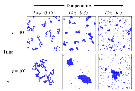
Figure 2: Snapshots of configurations at three representative temperatures. At $\epsilon_{\mathrm{b}}/T=0.15$ (low temperature), long-lived fractal clusters survive to form a stable gel-like structure, which we identify as kinetically frustrated. At $\epsilon_{\mathrm{b}}/T=0.5$ (a higher temperature) and for long times, the system fully phase separates into a large cluster surrounded by a dilute gas. However, the large cluster is not close-packed and a large proportion of particles remain in small clusters: this is therefore poor assembly. At $\epsilon_{\mathrm{b}}/T=0.35$ (intermediate temperature) the majority of the particles are in large clusters having few defects, which we identify as good assembly.

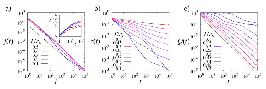
Figure 3: Plots of the flux $f(t)$ and traffic $\tau(t)$, and their ratio $Q(t)$. The flux varies little across the temperature range considered while the traffic depends much more strongly on the temperature. In the kinetic trapping regime $T/\epsilon_{\mathrm{b}}\lesssim 0.2$, the ratio $Q$ remains relatively large throughout the trajectories, while the good assembly and high-temperature regimes are associated with reversible evolution and small values of $Q$.

In studying the lattice gas we have in mind a system self-assembling (or phase separating) into an ordered phase such as a crystal, coexisting with a dilute fluid. In the ordered phase, particles have a specific local co-ordination environment. In the lattice gas model, we take this local environment to be that a particle has all neighbouring sites occupied. We define the ‘assembly yield’, $n_{4}(t)$, as the proportion of particles with the maximal number of $4$ bonds to neighbouring particles. In Fig. 1b we plot the average yield at two fixed times. We observe a maximum at a reduced temperature that we denote by $T^{*}/\epsilon_{\mathrm{b}}$: the value of $T^{*}$ depends only weakly on time $t$. The system shows three qualitative kinds of behaviour. To illustrate this, we show snapshots from our simulations in Fig. 2, at three representative bond strengths. For strong bonds, there is a decrease in yield as the system becomes trapped in kinetically frustrated states. For weak bonds, the system is already close to equilibrium at $t=10^{6}$ but the final state has a relatively low value of $n_{4}(t)$. In the language of self-assembly, we interpret this as a poor quality product. Based on Figs. 1 and 2, we loosely identify the kinetically trapped regime as $T/\epsilon_{\mathrm{b}}<0.2$ and the regime of weak bonding and poor assembly as $T/\epsilon_{\mathrm{b}}\geq 0.5$. However, we emphasise that these regimes are separated by smooth crossovers and not sharp transitions. In the following, we use $T/\epsilon_{\mathrm{b}}=0.15,0.35,0.5$ as representative state points for kinetic trapping, good assembly and poor assembly, respectively.

Thus, despite the simplicity of the lattice gas, it captures the kinetic trapping effects and the non-monotonic yield observed in more physically realistic model systems Hagan and Chandler (2006); Wilber et al. (2007); Whitelam et al. (2009); Jack et al. (2007); Rapaport (2008); Klotsa and Jack (2011); Grant et al. (2011). We emphasise that the kinetically trapped states we find are closely related to diffusion-limited aggregates Meakin (1983), while the ‘assembled’ states are compact clusters. The changes in cluster morphology on varying bond strength are discussed further in Hagan et al. (2011) but in this article we concentrate on the dynamical reversibility of assembly Whitesides and Boncheva (2002); Jack et al. (2007); Rapaport (2008); Klotsa and Jack (2011) and not on the structure of the clusters. We include in Fig. 1 the equilibrium behaviour for systems of this size, which we obtain by running dynamical simulations starting from a fully phase-separated state in which a single large cluster contains all particles. As $t\rightarrow\infty$, the yield must approach its equilibrium result: the laws of thermodynamics state that if we wait long enough then the highest quality assembly (or the lowest energy final state) will be at the lowest temperature.

III Measuring Reversibility

III.1 Flux-Traffic Ratio

We now turn to measurements of reversibility and their relation to kinetic trapping effects and the non-monotonic yield shown in Fig. 1. We follow Grant et al. (2011) in considering the net rate of energy changing events at a microscopic level, the flux, in proportion to the total rate of energy changing events, the traffic (see also Lecomte et al. (2007); Garrahan et al. (2009); Baiesi et al. (2009)). We count an event (or ‘kink’) whenever a particle changes its number of neighbours: the number of times that particle $i$ increases its number of bonds between times $t$ and $t+\Delta t$ is $K^{+}_{p}(t,\Delta t)$, with $K^{-}_{p}(t,\Delta t)$ the number of times the particle decreases its number of bonds. We then average and normalise by the time interval

$$k^{\pm}(t,\Delta t)=\frac{1}{\Delta t}\langle K_{p}^{\pm}(t,\Delta t)\rangle.$$ (2)

Here and throughout, averages $\langle\dots\rangle$ run over the stochastic dynamics of the system and over a distribution of initial configurations where particle positions are chosen independently at random. In the limit $\Delta t\rightarrow 0$, then the $k^{\pm}(t,\Delta t)$ converge to the rates for bond-breaking ($+$) and bond-making ($-$) events, which we denote by $k^{\pm}(t)$. The flux, $f(t)=k^{+}(t)-k^{-}(t)$ is the net rate of bond-making and the traffic is the total rate of all events $\tau(t)=k^{+}(t)+k^{-}(t)$. (In contrast to Grant et al. (2011), we focus here on rates for making and breaking bonds and not on the total numbers of bonds made or broken.)

We also define a flux-traffic ratio

$$Q(t)=\frac{f(t)}{\tau(t)}$$ (3)

which provides a dimensionless measure of the instantaneous reversibility of a system, consistent with the qualitative description of reversibility due to Whitesides Whitesides and Boncheva (2002). The inverse of the flux-traffic ratio $1/Q(t)$ is the number of energy changing events per net bonding event. In a system at equilibrium $f(t)=0$ and so $Q(t)=0$ also. For a system quenched to $T=0$, our MC dynamics does not permit bonds to be broken so particles never increase their energy: hence $k^{-}(t)=0$ and $Q(t)=1$. In systems that have been quenched, we expect to see a value between these two limits, $0<Q(t)<1$: the smaller the flux-traffic ratio the ‘more reversible’ the system, while large flux-traffic ratios permit more rapid assembly.

In Fig. 3 we plot the flux $f(t)$, traffic $\tau(t)$, and their ratio $Q(t)$ at a range of bond strengths, $2<\epsilon_{\mathrm{b}}/T<10$. In all cases, the flux decreases towards zero as the system evolves towards equilibrium. On this logarithmic scale, the temperature-dependence of the flux appears quite weak, although the difference between different bond strengths may be up to an order of magnitude. Given that the ‘integrated flux’ ${\cal F}(t)=\int_{0}^{t}\mathrm{d}t^{\prime}f(t^{\prime})$ Grant et al. (2011)(Fig.3a inset) is always less than the maximal number of possible bonds ($4$ in this case), it is clear that $f(t)\lesssim t^{-1}$ at long times.

In contrast to the flux, the traffic shows a large variation with bond strength. Weaker bonds are more easily broken and result in more traffic. Combining flux and traffic, the ratio $Q(t)$ is less than $0.1$ throughout the good assembly regime, and decreases approximately as $t^{-1}$ while good assembly is taking place. The regime of kinetic trapping is characterised by larger values of $Q(t)$ and weaker time dependence. Similar results were found in Ref. Grant et al. (2011), where a similar ratio denoted by $\tilde{M}$ was used to compare total numbers of bond-breaking and bond-making events. Compared to $\tilde{M}$, the ratio $Q(t)$ depends only on the state of the system at time $t$ and not on its history: this will be useful in making contact with other measures of reversibility to be discussed below. The ratio $1/Q(t)$ is in the range $10-1000$ during optimal assembly, indicating (as in Grant et al. (2011)) that the system makes many steps forwards and backwards before it achieves a single step of net progress towards the assembled state. In this sense, good assembly requires significant reversibility, as argued above.

III.2 ‘Flux relation’ between correlation and response functions

In designing and controlling self-assembly processes, it would be useful if reversibility could be measured and controlled, to avoid kinetic trapping effects. While flux and traffic observables are not readily measured except in simple simulation models, we now show how correlation and response functions can be used to reveal similar information (see also Jack et al. (2007); Klotsa and Jack (2011)). These functions can be measured without the requirement to identify specific bonding and unbonding events; in some cases correlations and responses can also be calculated experimentally Jabbari-Farouji et al. (2007); Maggi et al. (2010); Oukris and Israeloff (2010).

At equilibrium, fluctuation dissipation theorems (FDTs) Chandler (1987) allow the response of a system to an external perturbation to be calculated from correlation functions measured in the absence of the perturbation. Away from equilibrium, such comparisons may be used for a classification of aging phenomena Crisanti and Ritort (2003) and may also be useful for estimating the degree of (ir)reversibility in self-assembling systems Jack et al. (2007); Klotsa and Jack (2011).

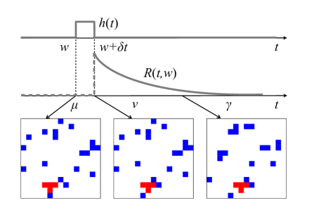
Figure 4: Procedure for measuring the impulse response. The system is initialised in a random configuration. After a waiting time, $w$, a perturbation is applied for a single MC move during which the system attempts a move from configuration $\mu$ to $\nu$. The field is then switched off and the system allowed to evolve until time $t$, at which point its configuration is denoted by $\gamma$. The typical response of the system is indicated, together with snapshots of showing how particles might move through the system. (The cluster that moves in the step while the perturbation is applied is highlighted in red.)

Figure 5: Data for $\tilde{S}_{\Delta t}(t,w)$, $\tilde{R}_{\Delta t}(t,w)$ and $\tilde{\Delta}_{\Delta t}(t,w)$ at three representative temperatures. The data are obtained at fixed $w=10^{3}$ MCS, while the time $t$ is varied. The deviation between correlation $S(t,w)$ and response $R(t,w)$ is small in both good assembly and poor assembly regimes, but significant in the kinetically frustrated regime. We emphasise that the correlation and response functions are associated with perturbations to particle bond strengths: that is, $A=B=n_{p}$ in the definitions of $S$ and $R$.

We first consider the general case for measurement of a response function in a system with MC dynamics. Fig. 4 illustrates our notation and the procedure used. The system is initialised at $t=0$ and evolves up to time $w$, when a perturbing field of strength $h$ is switched on. A single MC move is attempted with the field in place, after which the field is switched off. The system evolves with unperturbed dynamics up to a final time $t$ at which an observable $A$ is measured. In general, the response function depends on the two times $t$ and $w$ and gives the change in the average value of $A$, in response to the small field $h$. As indicated in Fig. 4, we use Greek letters to represent configurations of the system. (Recall that $\delta t$ is the time associated with a single MC move.)

The MC scheme may be specified through the probabilities $P^{0}(\nu\leftarrow\mu)$ for transitions from configuration $\mu$ to $\nu$ in a single attempted move. However, it is convenient to work with transition rates $W^{0}(\nu\leftarrow\mu)=(\delta t)^{-1}P^{0}(\nu\leftarrow\mu)$. We also define $\rho_{w}(\mu)$ as the probability that the system is in the specific configuration $\mu$ at time $w$, and the propagator $G^{0}_{t}(\nu\leftarrow\mu)$ as the probability that a system initially in state $\mu$ will evolve to state $\nu$ over a specified time period $t$. The superscripts $0$ indicate that no perturbation is being applied to the system: we use a superscript $h$ if the field is applied. [It follows that $\rho_{w}(\mu)=\sum_{\kappa}G^{0}_{w}(\mu\leftarrow\kappa)\rho_{0}(\kappa)$ where $\rho_{0}(\kappa)$ is the probability of initial condition $\kappa$ in the dynamical simulations.]

With these definitions, the average value of the observable $A$ at time $t$ is

$$\langle A(t)\rangle=\sum_{\gamma\mu\nu}A(\gamma)G^{0}_{u}(\gamma\leftarrow\nu)P^{h}(\nu\leftarrow\mu)\rho_{w}(\mu),$$ (4)

where $A(\gamma)$ is the value of $A$ in configuration $\gamma$ and we introduce $u\equiv t-w-\delta t$ for compactness of notation. (Since we use Greek letters to represent configurations, there should be no confusion between $A(\gamma)$ and $\langle A(t)\rangle$, the former being a property of configuration $\gamma$ and the latter a time-dependent average.) The definition of the (impulse) response is

$$R(t,w)\equiv\frac{T}{\delta t}\frac{\partial\langle A(t)\rangle}{\partial h},$$ (5)

where the derivative is evaluated at $h=0$. Hence,

$$R(t,w)=T\sum_{\gamma\nu\mu}A(\gamma)G^{0}_{u}(\gamma\leftarrow\nu)\frac{\partial}{\partial h}W^{h}(\nu\leftarrow\mu)\rho_{w}(\mu).$$ (6)

We assume that the system obeys detailed balance with respect to an energy function $E^{h}=E^{0}-hB$ where $E^{0}$ is the energy of the unperturbed system and $B$ is the conjugate observable to the field $h$. It is convenient to define a connected correlation function

$$C(t,w)=\langle\delta A(t)\delta B(w)\rangle$$ (7)

(here and throughout we use the notation $\delta O=O-\langle O\rangle$ for all observables $O$). We also define

$$S(t,w)\equiv\frac{\partial}{\partial w}C(t,w).$$ (8)

[The MC dynamics evolves in discrete time steps: the interpretation of the time-derivative is discussed in Appendix A.] At equilibrium, one has the FDT

$$R^{\mathrm{eq}}(t,w)=S^{\mathrm{eq}}(t,w).$$ (9)

Out of equilibrium, we define

$$\Delta(t,w)\equiv S(t,w)-R(t,w)$$ (10)

as a deviation between the response of the actual system and the response of an equilibrated system with the same correlation functions.

Various out-of-equilibrium expressions for response functions may be derived: see for example Baiesi et al. (2009); Seifert and Speck (2010); Corberi et al. (2010) where different representations are defined and compared with each other. In Appendix A.1, we give a proof of (9) and we derive the general relation

$$\Delta(t,w)=\sum_{\gamma\nu\mu}[A(\gamma)-\langle A(t)\rangle]G_{u}(\gamma\leftarrow\nu)F(\nu,\mu)J^{0}_{w}(\nu,\mu)$$ (11)

where

$$F(\nu,\mu)=T\frac{\partial}{\partial h}\ln W^{h}(\mu\leftarrow\nu)$$ (12)

and

$$J^{0}_{w}(\mu,\nu)=W^{0}(\nu\leftarrow\mu)\rho_{w}(\mu)-W^{0}(\mu\leftarrow\nu)\rho_{w}(\nu)$$ (13)

is the probability current between configurations $\mu$ and $\nu$ at time $w$. We will see below that the probability current $J^{0}$ plays a central role in quantifying irreversibility and deviations from equilibrium.

The formula (11) is general for discrete time Markov processes obeying detailed balance (the generalisation to Markov jump processes in continuous time is straightforward). We emphasise that (11) is a representation of (6), valid whenever detailed balance holds. As such, it is mathematically equivalent to several other representations that have been derived elsewhere: for example, the ‘asymmetry’ function discussed by Lippiello et al. Lippiello et al. (2005); Corberi et al. (2010) plays a role similar to $\Delta(t,w)$ in the case of Langevin processes. The purpose of (11) is to make contact between reversibility and deviations from FDT in self-assembling systems, as we now discuss. Further details of the relation between (11) and previous analyses Chatelain (2004); Ricci-Tersenghi (2003); Lippiello et al. (2005); Baiesi et al. (2009); Seifert and Speck (2010); Corberi et al. (2010) are discussed in Sec. III.7 below.

III.3 Energy correlation and response functions in the lattice gas

We now turn to response functions in the lattice gas. We consider how a single particle in the lattice gas responds if the strength of its bonds are increased. To this end, we write the energy in the presence of perturbing fields $h_{p}$ as $E^{h}=\sum_{p}[\frac{1}{2}\epsilon_{\mathrm{b}}-h_{p}]n_{p}$ where the sum runs over all particles, as in (1). We measure the response of $\langle n_{p}\rangle$ to the field $h_{p}$, by taking the observables $A$ and $B$ of the previous section both equal to the number of bonds $n_{p}$ for a specific particle $p$. Thus $R(t,w)=\frac{T}{\delta t}\frac{\partial\langle n_{p}\rangle}{\partial h_{p}}$. Given the energy function $E^{h}$, there is still considerable freedom to choose the MC rates $W^{h}$ while preserving detailed balance.

In Lippiello et al. (2005); Baiesi et al. (2009); Corberi et al. (2010), it was mathematically convenient to take $W^{h}(\nu\leftarrow\mu)=W^{0}(\nu\leftarrow\mu)\mathrm{e}^{h[B(\mu)-B(\nu)]/2}$. Here our dynamics we are motivated by the central assumptions (i) and (ii) of Sec. II.1, which indicate that rates for bond-making and cluster diffusion should depend only weakly on perturbations to the particle bond strengths. We therefore include all $h$-dependence in the probability $P_{\mathrm{a}}^{h}$ of accepting an MC move, as follows. If the change in the unperturbed energy for an MC move is $\Delta E^{0}$ and the change in the perturbation is $\Delta V=-\sum_{p}h_{p}\Delta n_{p}$ then for $\Delta E^{0}\neq 0$ we take take $P_{\mathrm{a}}^{h}=\mathrm{min}(1,\mathrm{e}^{(\lambda-1)\Delta E^{0}/T-\Delta V/T})$ while for $\Delta E^{0}=0$ we take $P_{\mathrm{a}}^{h}=2\alpha/(1+\mathrm{e}^{\Delta V/T})$. It is easily verified that this choice is compatible with detailed balance and reduces to the unperturbed probabilities $P_{\mathrm{a}}$ if $\Delta V=0$. Further, coupling the field $h_{p}$ only to the acceptance probability ensures that the perturbation affects the rates for bond-breaking and bond-making but does not affect the rates for diffusion of whole clusters.

We use a straightforward generalisation of the ‘no-field’ method Chatelain (2004); Ricci-Tersenghi (2003) to allow efficient measurement of the response: see Appendix A.2 for details. To attain good statistics, we consider responses in which the perturbing field $h$ acts not just for one MC move but for a time interval $\Delta t=10$ MC sweeps. Since we are working at leading order in $h$, the response to such a perturbation is simply

$$R_{\Delta t}(t,w)\equiv\frac{\delta t}{\Delta t}\sum_{j=0}^{(\Delta t/\delta t)-1}R(t,w+j\delta t).$$ (14)

The relevant correlation function in this case is $C(t,w)=\langle\delta n_{p}(t)\delta n_{p}(w)\rangle$ where $\delta n_{p}(t)=n_{p}(t)-\langle n_{p}(t)\rangle$ as usual. It is convenient to define normalised correlation and response functions

$$\tilde{S}_{\Delta t}(t,w) =\frac{1}{{\cal N}_{\Delta t}(w)}[C(t,w+\Delta t)-C(t,w)]$$ (15)

$$\tilde{R}_{\Delta t}(t,w) =\frac{1}{{\cal N}_{\Delta t}(w)}R_{\Delta t}(t,w)$$ (16)

with ${\cal N}_{\Delta t}(w)=C(w+\Delta t,w+\Delta t)-C(w+\Delta t,w)$ so that $\tilde{S}_{\Delta t}(w+\Delta t,w)=1$. We also define

$$\tilde{\Delta}_{\Delta t}(t,w)=\tilde{S}_{\Delta t}(t,w)-\tilde{R}_{\Delta t}(t,w).$$ (17)

In all cases, the subscript $\Delta t$ indicates that these functions generalise the $R(t,w)$, $S(t,w)$ and $\Delta(t,w)$ of the previous section, while the tilde indicates normalisation. For small $\Delta t$, the dependence of these functions on $\Delta t$ is weak, but numerical calculation of the response is easier for larger $\Delta t$.

In Fig. 5 we show numerical results for correlation and response functions. At $T/\epsilon_{\mathrm{b}}=0.5$, clusters of particles are growing in the system, which is far from global equilibrium. However, as found in Jack et al. (2007); Klotsa and Jack (2011) for several other self-assembling systems, the deviations from FDT are small because the time-evolution is nearly reversible (recall Fig. 3). On the other hand, at $T/\epsilon_{\mathrm{b}}=0.15$, the particles are aggregating in disordered clusters and the time evolution is far from reversible with unbonding events being rare.

The potential utility of this result was discussed in Jack et al. (2007); Klotsa and Jack (2011): it means that straightforward measurements on short time scales can be used to predict long-time assembly yield, by exploiting links between correlation-response measurements and reversibility. In what follows, we explore in more detail how the deviation function $\Delta$ couples to microscopic irreversibility during assembly.

III.4 Interpretation of $\Delta(w+\delta t,w)$ as a flux

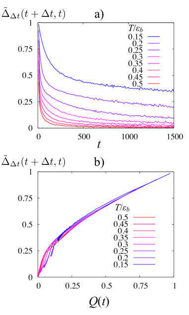
Figure 6: a) The deviation from FDT measured immediately after perturbation, $\tilde{\Delta}_{\Delta t}(t+\Delta t,t)$, $\Delta t=10$. At temperatures above $T^{*}$, $\tilde{\Delta}_{\Delta t}(t+\Delta t,t)$ decreases quickly with $t$, while at low temperatures it remains significant throughout the early times. In the construction of $\Delta(t,w)$ we take the observables to be $A=B=n_{p}$ as discussed in the main text. (b) Parametric plot of $\tilde{\Delta}_{\Delta t}(t+\Delta t,t)$ against the flux-traffic ratio $Q(t)$, for $0<t<1500$. The relationship between these two quantities depends very weakly on temperature, indicating the close relation between them.

In this section, we concentrate on quantities that can be written in the form

$$Z(t)=\sum_{\mu\nu}z(\nu,\mu)J^{0}_{t}(\nu,\mu)$$ (18)

where $J^{0}_{w}$ is the probability current, defined in (13). In contrast to straightforward one-time observables like $\langle A(t)\rangle=\sum_{\mu}A(\mu)\rho_{t}(\mu)$, we will show that observables like $Z(t)$ are currents, time-derivatives and fluxes: they measure deviations from instantaneously reversible behaviour, measured at time $t$.

To this end, we generalise the analysis of “kinks” in Sec. III.1 by defining $\langle K^{\nu\mu}(t,\Delta t)\rangle$ as the average number of MC transitions from state $\mu$ to state $\nu$ between times $t$ and $t+\Delta t$. The associated kink rate is $k^{\nu\mu}(t)=(\delta t)^{-1}\langle K^{\nu\mu}(t,\delta t)\rangle$. It follows from the definition of the $k$s that

$$k^{\nu\mu}(t)-k^{\mu\nu}(t)=J^{0}_{t}(\nu,\mu)$$ (19)

Thus, the probability current $J^{0}_{t}$ gives the difference between the probabilities of forward and reverse MC transitions between states $\mu$ and $\nu$, which clarifies its connection to irreversibility. At equilibrium, one has $J^{0}_{t}(\nu,\mu)=0$ for all states $\mu$ and $\nu$: thus, $J^{0}_{t}$ measures deviations from equilibrium. However, measuring (or even representing) $J^{0}_{t}$ is a near-impossible task in a system where the number of possible states $\mu$ is exponentially large in the system size.

Instead, one makes a specific choice of the $z(\nu,\mu)$, in which case (18) shows that $Z(t)$ is a projection of the current $J^{0}_{t}$ onto the observables of the system. For example, if $z(\nu,\mu)=A(\nu)$ then $Z(t)=\frac{\partial}{\partial t}\langle A(t)\rangle$ is a time derivative that clearly vanishes at equilibrium (or in any steady state). Other choices for $z(\nu,\mu)$ become relevant in out-of-equilibrium settings. For example, the flux $f(t)$ in Sec. III.1 is obtained by setting $z(\nu,\mu)=1$ if the transition $\mu\to\nu$ involves an increase in the number of bonds of particle $p$, with $z(\nu,\mu)=0$ for all other $\mu,\nu$. (The structure of (18) together with this choice of $z$ ensures that $f(t)$ acquires negative contributions from MC transitions where particle $p$ experiences a decrease in its number of bonds, as required.) Similarly the particle current in exclusion processes is obtained by taking $z(\nu,\mu)=1$ for transitions $\mu\to\nu$ where a particle hops to the right, and zero for all other pairs. Clearly, these observables monitor the breaking of time-reversal symmetry, as is the case for all observables $Z(t)$.

To relate deviations from FDT to irreversible events, we first consider the case $t=w+\delta t$, so that the perturbation $h$ is applied for just one MC move and then the response is measured immediately. In this case (11) reduces to

$$\Delta(w+\delta t,w)=\sum_{\nu,\mu}z_{\Delta}(\nu,\mu)J_{w}^{0}(\nu,\mu)$$ (20)

as in (18), with

$$z_{\Delta}(\nu,\mu)=[A(\nu)-\langle A(w+\delta t)\rangle]F(\nu,\mu).$$ (21)

The function $F(\nu,\mu)$ was defined in (12) and measures the effect of the perturbation $h$ on the transition rate from $\nu$ to $\mu$. The factor $A(\nu)-\langle A(w+\delta t)\rangle$ indicates whether configuration $\nu$ has a high or a low value of the observable $A$, compared to the average of $A$ at the measurement time $w+\delta t$.

For the case considered in Sec. III.3 and Fig. 5, where the perturbation is coupled to the energy of particle $p$, one has $A(\nu)=n_{p}(\nu)$ and

$$F(\nu,\mu)=[n_{p}(\nu)-n_{p}(\mu)]\Theta(E^{0}(\mu)-E^{0}(\nu))$$ (22)

where $\Theta(x)$ is the step function, defined such that $\Theta(0)=\frac{1}{2}$. The step function appears because if a proposed MC move results in a decrease in the bare energy, the acceptance probability does not depend on the perturbing field $h_{p}$. Clearly, $F(\nu,\mu)$ is finite only if particle $p$ changes its energy between states $\mu$ and $\nu$: the same is true for $z_{\Delta}(\mu,\nu)$.

Thus, (20) indicates that the deviation $\Delta(t,w)$ measured at $t=w+\delta t$ reflects the imbalance between rates of bond-making and bond-breaking for particle $p$. In this respect it is similar to the flux $f(w)$: however, the weights given to different bond-making and bond-breaking processes differ between $\Delta(w+\delta t,w)$ and $f(w)$, due to the different forms of $z(\nu,\mu)$ in the two cases. Thus, while these quantities reflect similar physics, the details of their behaviour is different. To see the relationship between the immediate response $\Delta(w,w+\delta t)$ and the flux $f(t)$ from Sec. III.1, we present Fig. 6 which shows that the two quantities have similar time and temperature-dependence and therefore reveal similar information about the (ir)reversibility of the dynamical bonding and unbonding processes.

III.5 Time intervals for reversibility

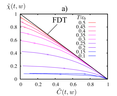
Figure 7: Integrated correlation-response plot showing the response $\tilde{\chi}(t,w)$ and correlation $\tilde{C}(t,w)$. The correlation and response functions are associated with observables $A=B=n_{p}$, as in previous figures. The data is shown for a fixed $t=10^{4}$ MCS and and $0\leq w<t$. The $\times$ symbol indicates the points where $w=10^{3}$: impulse responses associated with this time are shown in Fig. 5.

We now consider the deviation $\Delta(t,w)$ for $t>w+\delta t$. From (11), we see that $\Delta(t,w)$ can be written in the form (18) if we take

$$z(\nu,\mu)=[\mathcal{P}^{A}_{u}(\nu)-\langle A(t)\rangle]F(\nu,\mu).$$ (23)

where

$${\cal P}^{A}_{u}(\nu)=\sum_{\gamma}A(\gamma)G^{0}_{u}(\gamma\leftarrow\nu)$$ (24)

is the propensity Widmer-Cooper et al. (2004) of observable $A$ for configuration $\nu$ after a time $u$. That is, ${\cal P}^{A}_{u}(\nu)$ is the value of $A$ that is obtained by an average over the dynamics of the system, for a fixed initial condition $\nu$ and a fixed time $u$. (Recall $u=t-w-\delta t$.)

Comparing (23) with (21), the difference is the replacement of $A(\nu)$ by the propensity. At equilibrium, one expects $\mathcal{P}^{A}_{u}(\nu)-\langle A(t)\rangle$ to decay towards zero as $u$ increases, since the system forgets its memory of the configuration $\nu$ and “regresses back to the mean”. (That is, the propensities for different fixed initial conditions all converge to the same average value at long times.) Out of equilibrium, this may not be the case: if a configuration $\nu$ has a more ordered structure than another configuration $\nu^{\prime}$ then these configurations may have different propensities for order even at much later times. Loosely, a system in $\nu$ has a ‘head start’ along the route to assembly, and the system does not forget the memory of this head start as assembly proceeds.

Fig. 5 shows that for the correlation and response functions considered here, the deviation $\Delta(t,w)$ decays only very slowly with time $t$. The $t$-dependence of this function comes through a weighted sum of propensities: it is therefore clear that these propensities do not regress quickly to the mean. In contrast, one may write the correlation as

$$S(t,w)=\sum_{\nu\mu}[{\cal P}_{u}^{A}(\nu)-\langle A(t)\rangle][n_{p}(\nu)-n_{p}(\mu)]\\ \times W^{0}(\nu\leftarrow\mu)\rho_{w}(\mu)$$ (25)

whose $t$-dependence also comes from the propensity. Fig. 5 shows that this function does decay quite quickly with $t$, although it does not reach zero on the time scales considered here.

Our conclusion is the following. For configurations $\nu$ that are typical at time $w$, the propensity ${\cal P}_{u}^{A}(\nu)$ has a ‘fast’ contribution that decays quickly with time $u$, as well as a ‘slow’ contribution that depends weakly on $u$ and reflects the ‘head start’ of $\nu$ along the route to the assembled product. The fast contribution reflects rapid bond-making and bond-breaking events that do not lead directly to assembly while the ‘slow’ contribution is a non-equilibrium effect that measures assembly progress and also dominates the deviation $\Delta(t,w)$ that we have defined here. By contrast $S(t,w)$ picks up contributions from both slow and fast contributions. The utility of the FDR is that for suitable $w$, it couples to the irreversible bond-making behaviour that is most relevant for self-assembly.

To illustrate this balance of fast and slow degrees of freedom, and also to make contact with previous studies Crisanti and Ritort (2003); Jack et al. (2007); Klotsa and Jack (2011) of FDRs, we define an integrated (and normalised) response

$$\tilde{\chi}(t,w)=\frac{1}{C(t,t)}\int_{w}^{t}\!\mathrm{d}w^{\prime}R(t,w^{\prime})$$ (26)

and we also normalise the correlation as

$$\tilde{C}(t,w)=\frac{C(t,w)}{C(t,t)}$$ (27)

It is conventional to display these correlations functions in a parametric form Crisanti and Ritort (2003). Specifically, making a parametric plot of $\tilde{\chi}(t,w)$ against $\tilde{C}(t,w)$, for fixed $t$ and varying $w$, the gradient is $-X(t,w)$. It has been emphasised several times Sollich et al. (2002); Jack et al. (2006); Russo and Sciortino (2010) that plotting data for fixed $w$ and varying $t$ is not in general equivalent to this procedure and may give misleading results, especially if $C(t,t)$ has significant time-dependence, as it does in these systems. Plotting data at fixed $t$ as in Fig. 7, it is apparent that the high temperature systems are the most reversible, with $X(t,w)\approx 1$. To understand the connection with Fig. 5, note that the time interval $t-w$ increases from right to left in Fig. 7: when $t-w$ is large then the deviation $\Delta(t,w)$ has a larger fractional contribution to $S(t,w)$, so that the curves are steepest (most reversible) when $t-w$ is small and least steep (least reversible) when $t-w$ is large. We find that parametric plots depend weakly on the fixed values of $t$ used but we do not show this data, for brevity: see for example Ref. Klotsa and Jack (2011) for an analysis of $t$-dependence in a system of crystallising particles.

Physically, we attribute the $w$-dependence of $X(t,w)$ to the fact that fast degrees of freedom (like dimer formation and breakage in the vapour phase) quickly relax to a quasiequilibrium state Hagan et al. (2011) where probability currents $J^{0}$ associated with this motion are small. It is only much slower degrees of freedom (like the gradual growth/assembly of large clusters) for which probability currents remain significant on long time scales, and lead to long-time contributions to $\Delta(t,w)$.

Compared to the simple flux-traffic ratio $Q(t)$ considered in Sec. III.1, the normalised deviation $1-X(t,w)=\Delta(t,w)/S(t,w)$ has the same effect of comparing a generalised flux $\Delta(t,w)$ with a normalisation $S(t,w)$ that reflects the traffic in the system. However, the effect of the time difference $t-w$ is that while $\Delta(t,w)$ decays slowly with time $t$ then $S(t,w)$ decays quite quickly. Thus, as $t$ increases, the deviation $1-X(t,w)$ becomes increasingly sensitive to the deviations from reversibility, since the fluctuations of fast (reversible) degrees of freedom regress back to the mean while the slow (irreversible) ones remain significant. For this reason, the FDR $X(t,w)$ is a more sensitive measure of irreversibility than the flux-traffic ratio discussed in Sec. III.1.

III.6 Responses to different perturbations

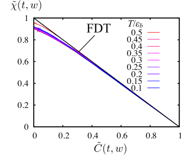
Figure 8: Integrated correlation-response plot a site dependent perturbation. That is, we take the observables $A=B=\rho_{i}$ as described Sec. III.6, and in contrast to previous figures where $A=B=n_{p}$. The data is shown for fixed $t=10^{4}$ with $\times$ symbols indicating $w=10^{3}$, as in Fig. 7. The relaxation of the observable $\rho_{i}$ is diffusive and depends weakly on the bond strength, so the dependence on $T/\epsilon_{\mathrm{b}}$ is much weaker than in Fig. 7 and the deviations from FDT behaviour are smaller.

We remark that the observables used in measuring correlation and response functions may strongly affect the results. Most relevant is the extent to which the response function couples to the slow, irreversible degrees of freedom and the fast, reversible ones. To illustrate this, we compare the results of the previous section with a different response function. We take the observables $A$ and $B$ of Sec. III.2 both equal to the occupancy $\rho_{i}=0,1$ of a specific site $i$ on the lattice. The effect of the perturbation on the MC dynamics is the same as that described in Sec. III.3, except that the perturbed energy $E^{h}=E^{0}+V$ with $V=\sum_{i}h_{i}\rho_{i}$, where the sum runs over sites of the lattice.

Unlike the bond numbers $n_{p}$ which change only when bonds are made and broken, the site occupancies $\rho_{i}$ also change as clusters diffuse through the system. When bonds are strong, the site correlation functions decay faster than the bond correlation functions considered above. Therefore, since the site response is coupling to fast degrees of freedom, we expect to see ‘more reversible’ behaviour: this is borne out by Fig. 8 where the FDRs are much closer to the equilibrium value (unity) than the FDRs shown in Fig. 7. This is consistent with recent results of Russo and Sciortino Russo and Sciortino (2010) who observed a similar effect, and with earlier studies of observable-dependence of FDRs Sollich et al. (2002); Mayer et al. (2003); Jack et al. (2006) (see however Mayer and Sollich (2005) in which some fast degrees of freedom do not relax to quasiequilibrium).

Similar correlation and response measurements in an Ising lattice gas were also considered by Krząkała Krzakala (2005), but the dynamical scheme used in that work means that clusters of particles do not diffuse: in that case the site degrees of freedom $\rho_{i}$ are not able to reach quasi-equilibrium and one does observe significant deviations from FDT for this observable.

We end this section by briefly considering these correlation and response functions for large $t$. In this limit, standard arguments Crisanti and Ritort (2003) indicate that both correlation and response functions have contributions from well-separated fast and slow sectors, with the contributions from the fast sector obeying FDT. In coarsening systems like this one then there is no response in the slow sector. Thus, for large enough times, the parametric plot has a segment with $X=1$ for large $C$ and small $\chi$; for smaller $C$ then $X=0$ so the parametric plot has a plateau where the value of $\chi(t,w)$ depends only on equilibrium properties of the system. However, we emphasise that the approach to this large-$t$ limit is very slow and applies only after all clusters in the system are annealed into compact clusters. This limit is therefore irrelevant for analysing the kinetic trapping phenomena on which we focus in this article.

III.7 Relation to previous analyses of non-equilibrium response

We have emphasised throughout this article that our main purpose is to use correlation and response measurements to measure reversibility in assembling systems. Many other studies have considered such measurements in a variety of other contexts – here we make connections between our methodology and some other results from the literature.

One recent area of interest has been the use of ‘no-field’ measurements of response functions. Here, the aim is to develop formulae for the response that can be evaluated in Monte Carlo simulations without the introduction of any direct perturbation Chatelain (2004); Ricci-Tersenghi (2003); Lippiello et al. (2005); Jack et al. (2006); Corberi et al. (2010). In fact, we use such a straightforward generalisation of the method of Chatelain (2004) to measure responses in this paper, as discussed in Appendix A.2.

Our analysis in Sec. III.2 is concerned not so much with measurement of the response, but with the physical interpretation of deviations from FDT. Our result is therefore in the same spirit as Cugliandolo et al. (1997a, b); Crisanti and Ritort (2003); Lippiello et al. (2005); Jack et al. (2007); Baiesi et al. (2009); Seifert and Speck (2010). In particular, Baiesi et al Baiesi et al. (2009) relate the FDT to ‘flux’ and ‘traffic’ observables that separate reversible and irreversible behaviour, but they use a different approach to ours. Full details are given in Appendix. A.3 but in our notation, their central result is

$$R(t,w)=\frac{1}{2}\left[\frac{\partial}{\partial w}\langle A(t)B(w)\rangle+\langle A(t)\mathcal{T}(w)\rangle\right]$$ (28)

where $\mathcal{T}(w)$ measures the $h$-dependence of the amount of dynamical activity (traffic) between times $w$ and $w+\delta t$. The second term is therefore associated with traffic while the first term is a correlation between $A(t)$ and the ‘excess entropy production’ at time $w$: it is therefore related to a flux. However, neither of the correlation functions in (28) may be written in the form of (18) so they do not vanish at equilibrium. The key point is that in equilibrated (reversible) systems, the terms in (28) are both non-zero and equal to each other. So while (28) does involve a separation of terms symmetric and anti-symmetric under time reversal, the resulting correlation functions are not fluxes in the form of (18) and do not provide the same direct measurement of the deviation from reversibility given by $\Delta(t,w)$ in (11).

In another relation to irreversible behaviour, the analysis of Refs. Lippiello et al. (2005); Corberi et al. (2010) identifies an ‘asymmetry’ measurement which in our notation is

$$\mathcal{A}(t,w)=R(t,w)-\frac{1}{2}[S(t,w)+S(w,t)]$$ (29)

It follows from the fluctuation dissipation theory that this quantity vanishes in a system with time-reversal symmetry. Comparison with (10) also illustrates the similarity between $\mathcal{A}(t,w)$ and the deviation $\Delta(t,w)$. However, $\mathcal{A}(t,w)$ differs from $\Delta(t,w)$ since the deviation $\Delta(t,w)$ is a projection of $J^{0}_{w}$ and hence vanishes if the system is behaving reversibly at time $w$, regardless of what happens at later times. On the other hand, $\mathcal{A}(t,w)$ vanishes only if all trajectories between times $w$ and $t$ are equiprobable with their time-reversed counterparts. That is, time-reversal symmetry must hold throughout the interval between $w$ and $t$, and not just at time $w$.

IV Outlook

We have analysed the extent to which ideas of reversible bond-making are applicable to a phase separating lattice gas, which we used as a simplified model for a self-assembling system. The data of Figs. 1, 3 and 7 further support the idea that this system is relevant for studying self-assembly, since similar results have been presented for more detailed models of self-assembling systems Hagan and Chandler (2006); Jack et al. (2007); Rapaport (2008); Klotsa and Jack (2011); Grant et al. (2011).

The flux/traffic measurements of Sec. III.1 provide an intuitive picture of reversibility, while the picture based on the correlation-response formalism is more subtle. However, the central result (11) demonstrates an explicit link between measurements of response functions and irreversibility of bonding. Also, Figs. 5 and 7 do indicate that information about both short-time reversible and long-time irreversible behaviour can be obtained by considering the behaviour of correlation and response functions.

It has been argued that correlation-response measurements on short time scales might be used to predict long-term assembly yield, and even to control assembly processes. The work presented here places this objective on a firmer theoretical footing, and highlights the importance of using the right observable when probing irreversibility (compare Figs. 7 and 8); the interplay between fast ‘quasiequilibrated’ degrees of freedom and slow ‘irreversible’ bonding Hagan et al. (2011) also highlights the importance of choosing the right time scale for measuring these functions and predicting long-time assembly quality.

Appendix A Derivations of representations for response functions

A.1 Deviation function $\Delta(t,w)$

In this Section, we derive equation (11) which gives the deviation between the response $R(t,w)$ and the correlation function $S(t,w)$. Starting from (6), conservation of probability for the MC transition probabilities implies that $P^{h}(\mu\leftarrow\mu)=1-\sum_{\nu(\neq\mu)}P^{h}(\nu\leftarrow\mu)$, with a similar relation for the rates $W^{h}$. Using this in (6) gives

$$R(t,w)=T\sum_{\gamma,\nu\neq\mu}A(\gamma)G_{u}(\gamma\leftarrow\nu)\frac{\partial}{\partial h}J^{h}_{w}(\mu,\nu)$$ (30)

with

$$J^{h}_{w}(\mu,\nu)=W^{h}(\nu\leftarrow\mu)\rho_{w}(\mu)-W^{h}(\mu\leftarrow\nu)\rho_{w}(\nu)$$ (31)

which has the structure of a flux in probability from configuration $\mu$ to configuration $\nu$. This is related Seifert and Speck (2010) to an expression for the response originally due to Agarwal Agarwal (1972).

We now assume that the system obeys detailed balance:

$$W^{h}(\mu\leftarrow\nu)\mathrm{e}^{-E^{h}(\nu)/T}=W^{h}(\nu\leftarrow\mu)\mathrm{e}^{-E^{h}(\mu)/T}$$ (32)

where $E^{h}(\mu)=E^{0}(\mu)-hB(\mu)$ as defined in Sec. III.2. Hence, one has $\frac{\partial}{\partial h}\ln W^{h}(\nu\leftarrow\mu)=\Delta B(\nu,\mu)/T+\frac{\partial}{\partial h}\ln W^{h}(\mu\leftarrow\nu)$ with $\Delta B(\nu,\mu)=B(\nu)-B(\mu)$, so that

$$T\frac{\partial}{\partial h}J^{h}_{w}(\mu,\nu)=\Delta B(\nu,\mu)W^{0}(\nu\leftarrow\mu)\rho_{w}(\mu)\\ +TJ^{0}_{w}(\nu,\mu)\frac{\partial}{\partial h}\ln W^{h}(\mu\leftarrow\nu).$$ (33)

Inserting (33) into (30) gives two contributions to the response. The first contribution is $\frac{1}{\delta t}\langle A(t)[B(w+\delta t)-B(w)]\rangle$. In the notation of the main text, this is equal to $S(t,w)+\langle A(t)\rangle\frac{\partial}{\partial w}\langle B(w)\rangle$ where the time derivative is interpreted as a change between $w$ and $w+\delta t$, normalised by the time $\delta t$ for a single MC move. (Recall that we took time to be discrete in these MC models.)

At equilibrium, $J^{0}=0$ and $\frac{\partial}{\partial w}\langle B(w)\rangle=0$ so the only contribution to the response is $S(t,w)$ and the FDT (9) holds. The non-equilibrium contributions to $R(t,w)$ can be collected together to obtain (11) if one notes (i) that that $\sum_{\gamma}G^{0}_{u}(\gamma\leftarrow\nu)=1$ which follows from conservation of probability and the definition of $G^{0}$ and (ii) that

$$\sum_{\mu\nu}F(\nu,\mu)J^{0}_{w}(\nu,\mu)=\frac{\partial}{\partial w}\langle B(w)\rangle,$$ (34)

which follows from the detailed balance property of the $W^{h}$.

A.2 ‘No-field’ formula for the response

Another useful representation of the response function expresses it in terms of directly observable quantities in unperturbed simulations Chatelain (2004); Ricci-Tersenghi (2003) (this is the ‘path weight’ representation of Seifert and Speck (2010)).

The original ‘no-field’ method requires an extension for our system since the cluster MC algorithm we use means that the same transition $\nu\leftarrow\mu$ may take place via several possible computational routes. (For example, two MC moves may start from different seed particles but result in the same cluster being moved in the same direction). We use $P(\nu\xleftarrow{C}\mu)$ to represent the probability of an MC move from $\mu$ to $\nu$ by some route $C$. For $\nu\neq\mu$, the route $C$ is the choice of seed particle and sequence of steps by which the moving cluster is generated. If $\nu=\mu$ the route $C$ may involve the proposal of a move that is then rejected, or the proposal of a move where the cluster size exceeds $n_{\mathrm{max}}$, or would result in multiple-occupancy of a site.

Starting from (6), one writes

$$R(t,w)=T\sum_{\gamma,\nu,\mu,C}A(\gamma)G^{0}_{u}(\gamma\leftarrow\nu)\mathcal{R}(\nu,C,\mu)\\ \times P^{0}(\nu\xleftarrow{C}\mu)\rho_{w}(\mu).$$ (35)

where $\mathcal{R}(\nu,C,\mu)=\frac{1}{\delta t}\frac{\partial}{\partial h}\log W^{h}(\nu\xleftarrow{C}\mu)$. This result may be written as a simple expectation value

$$R(t,w)=T\langle A(t)\mathcal{R}(w)\rangle$$ (36)

where the key point is that the observable ${\cal R}(\nu,C,\mu)$ may be evaluated for any attempted MC move so that the correlation function in (36) may be calculated directly from an MC simulation with $h=0$. [This is in contrast to the current $J^{0}_{w}(\nu,\mu)$ which depends on the whole ensemble of evolving systems, so that the formula (30) cannot be evaluated directly by MC simulation.]

For the dynamical method described in this paper, the observable ${\cal R}(\nu,C,\mu)$ is given by ${\cal R}=[n_{p}(\nu)-n_{p}(\mu)]\Theta(E^{0}(\mu)-E^{0}(\nu))$ if the move is accepted, as in the main text $\Theta(0)=\frac{1}{2}$. If the move is rejected either because the cluster size $n$ exceeds $n_{\rm max}$ or the move would have resulted in overlapping particles ${\cal R}=0$. If however the move is legal but rejected when testing the move acceptance probability $P_{\rm a}$, then ${\cal R}=-[n_{p}(\nu)-n_{p}(\mu)]\Theta(E^{0}(\mu)-E^{0}(\nu))\times P_{\rm a}/(1-P_{\rm a})$.

A.3 An alternative formula for the response

In this section we clarify the connections between our results and those of Baiesi et al. Baiesi et al. (2009). The central identity in the derivation of Appendix A.1 is $\frac{\partial}{\partial h}\ln W(\nu\leftarrow\mu)=\Delta B(\nu,\mu)/T+\frac{\partial}{\partial h}\ln W(\mu\leftarrow\nu)$. Rearranging, one may write

$$\frac{\partial}{\partial h}\ln W(\nu\leftarrow\mu)=\Delta B(\nu,\mu)/2T\\ +\frac{1}{2}\frac{\partial}{\partial h}\ln[W(\mu\leftarrow\nu)W(\nu\leftarrow\mu)]$$ (37)

and substitution into (6) leads to

$$R(t,w)=\frac{1}{2}\sum_{\gamma\mu\nu}A(\gamma)G_{u}(\gamma\leftarrow\nu)\\ \times[\Delta B(\nu,\mu)+{\cal T}(\nu,\mu)]W(\nu\leftarrow\mu)\rho_{w}(\mu)$$ (38)

with ${\cal T}(\nu,\mu)=T\frac{\partial}{\partial h}\ln[W(\mu\leftarrow\nu)W(\nu\leftarrow\mu)]$. Equ. (38) is the translation of the central result of Baiesi et al. Baiesi et al. (2009) into our notation.

The key point here is that the two terms in square brackets in (38) have different symmetry properties. By definition of the first term, $\Delta B(\nu,\mu)=-\Delta B(\mu,\nu)$. Time-reversal of the trajectory flips the roles of $\nu$ and $\mu$ so that $\Delta B$ is ‘anti-symmetric under time-reversal’ and is related to the entropy current Baiesi et al. (2009). This means that the average of $\Delta B$ is zero in a time-reversal symmetric system. (Note however that $\Delta B$ itself is a fluctuating quantity and not zero in general: this is different from the probability current $J^{0}_{w}$ which is an ensemble-averaged property without fluctuations and is strictly equal to zero if time-reversal holds.) On the other hand ${\cal T}(\nu,\mu)={\cal T}(\mu,\nu)$ so ${\cal T}$ is ‘symmetric under time-reversal’ and measures dynamical activity, or traffic.

Despite the links between Equ. (38) and time-reversal symmetries, neither of the terms in (38) may be written as a flux in the form of (18). Noting that $S(t,w)$ is a connected correlation function, one may write

$$R(t,w)=\frac{1}{2}\left[S(t,w)+\langle A(t)\mathcal{T}(w)\rangle+\langle A(t)\rangle\frac{\partial}{\partial w}\langle B(w)\rangle\right]$$ (39)

where the final term vanishes in the non-equilibrium steady states considered in Baiesi et al. (2009) while $\mathcal{T}(w)$ is given by $(\delta t)^{-1}{\cal T}(\nu,\mu)$, evaluated with $\nu$ and $\mu$ being the configurations at times $w+\delta t$ and $w$ respectively. The key point is that the first two terms on the right hand side of (39) are equal to each other and both are non-zero at equilibrium. Hence neither of them is directly identifiable as a flux that is sensitive only to deviations from reversibility. Combining the first and third terms on the right hand side of (39) yields (28) of the main text.

References

- Whitesides and Grzybowski (2002) G. Whitesides and B. Grzybowski, Science 295, 2418 (2002).
- Glotzer and Solomon (2007) S. C. Glotzer and M. J. Solomon, Nat Mater 6, 557 (2007).
- Halley and Winkler (2008) J. D. Halley and D. A. Winkler, Complexity 14, 10 (2008).
- Leunissen et al. (2005) M. Leunissen, C. Christova, A. Hynninen, C. Royall, A. Campbell, A. Imhof, M. Dijkstra, R. van Roij, and A. van Blaaderen, Nature 437, 235 (2005).
- Grzybowski et al. (2009) B. A. Grzybowski, C. E. Wilmer, J. Kim, K. P. Browne, and K. J. M. Bishop, Soft Matter 5, 1110 (2009).
- Chung et al. (2010) S. Chung, S. Shin, C. Bertozzi, and J. De Yoreo, Proc. Natl. Acad. Sci. (USA) 107, 16536 (2010).
- Romano et al. (2010) F. Romano, E. Sanz, and F. Sciortino, J. Chem. Phys. 132, 184501 (2010).
- Fox et al. (1998) J. Fox, G. Wang, J. Speir, N. Olson, J. Johnson, T. Baker, and M. Young, Virology 244, 212 (1998).
- Hagan and Chandler (2006) M. F. Hagan and D. Chandler, Biophys. J. 91, 42 (2006).
- Wilber et al. (2007) A. W. Wilber, J. P. K. Doye, A. A. Louis, E. G. Noya, M. A. Miller, and P. Wong, J. Chem. Phys. 127, 085106 (2007).
- Kraft et al. (2009) D. J. Kraft, J. Groenewold, and W. K. Kegel, Soft Matter 5, 3823 (2009).
- Sacanna et al. (2010) S. Sacanna, W. T. M. Irvine, P. M. Chaikin, and D. J. Pine, Nature 464, 575 (2010).
- Ariga et al. (2008) K. Ariga, J. P. Hill, M. V. Lee, A. Vinu, R. Charvet, and S. Acharya, Sci. Technol. Adv. Mater. 9, 014109 (2008).
- Kershner et al. (2009) R. J. Kershner, L. D. Bozano, C. M. Micheel, A. M. Hung, A. R. Fornof, J. N. Cha, C. T. Rettner, M. Bersani, J. Frommer, P. W. K. Rothemund, et al., Nat Nano 4, 557 (2009).
- Rothemund (2006) P. W. K. Rothemund, Nature 440, 297 (2006).
- Brown et al. (2002) W. L. Brown, R. A. Mastico, M. Wu, K. G. Heal, C. J. Adams, J. B. Murray, J. C. Simpson, J. M. Lord, A. W. Taylor-Robinson, and P. G. Stockley, Intervirology 45, 371 (2002).
- Stupp (2010) S. I. Stupp, Nano Letters 10, 4783 (2010).
- Whitesides and Boncheva (2002) G. M. Whitesides and M. Boncheva, Proc. Natl. Acad. Sci. U.S.A. 99, 4769 (2002).
- Jack et al. (2007) R. L. Jack, M. F. Hagan, and D. Chandler, Phys. Rev. E 76, 021119 (2007).
- Rapaport (2008) D. C. Rapaport, Phys. Rev. Lett. 101, 186101 (2008).
- Whitelam et al. (2009) S. Whitelam, E. H. Feng, M. F. Hagan, and P. L. Geissler, Soft Matter 5, 1251 (2009).
- Klotsa and Jack (2011) D. Klotsa and R. L. Jack, Soft Matter 7, 6294 (2011).
- Grant et al. (2011) J. Grant, R. L. Jack, and S. Whitelam, J. Chem. Phys. 135, 214505 (2011).
- Cugliandolo et al. (1997a) L. F. Cugliandolo, J. Kurchan, and L. Peliti, Phys. Rev. E 55, 3898 (1997a).
- Cugliandolo et al. (1997b) L. F. Cugliandolo, D. S. Dean, and J. Kurchan, Phys. Rev. Lett. 79, 2168 (1997b).
- Crisanti and Ritort (2003) A. Crisanti and F. Ritort, J. Phys. A 36, R181 (2003).
- Hagan et al. (2011) M. F. Hagan, O. M. Elrad, and R. L. Jack, J. Chem. Phys. 135, 104115 (2011).
- Meakin (1983) P. Meakin, Phys. Rev. Lett. 51, 1119 (1983).
- Baxter (2002) R. J. Baxter, Exactly solved models in statistical mechanics (Academic Press, 2002).
- Whitelam and Geissler (2007) S. Whitelam and P. L. Geissler, J. Chem. Phys. 127, 154101 (2007).
- Lecomte et al. (2007) V. Lecomte, C. Appert-Rolland, and F. van Wijland, J. Stat. Phys. 127 (2007).
- Garrahan et al. (2009) J. P. Garrahan, R. L. Jack, V. Lecomte, E. Pitard, K. van Duijvendijk, and F. van Wijland, J. Phys. A 42, 075007 (2009).
- Baiesi et al. (2009) M. Baiesi, C. Maes, and B. Wynants, Phys. Rev. Lett. 103, 010602 (2009).
- Jabbari-Farouji et al. (2007) S. Jabbari-Farouji, D. Mizuno, M. Atakhorrami, F. C. MacKintosh, C. F. Schmidt, E. Eiser, G. H. Wegdam, and D. Bonn, Phys. Rev. Lett. 98, 108302 (2007).
- Maggi et al. (2010) C. Maggi, R. DiLeonardo, J. C. Dyre, and G. Ruocco, Phys. Rev. B 81, 104201 (2010).
- Oukris and Israeloff (2010) H. Oukris and N. E. Israeloff, Nature Physics 6, 135 (2010).
- Chandler (1987) D. Chandler, Introduction to Modern Statistical Mechanics (OUP, 1987).
- Seifert and Speck (2010) U. Seifert and T. Speck, EPL 89, 10007 (2010).
- Corberi et al. (2010) F. Corberi, E. Lippiello, A. Sarracino, and M. Zannetti, Phys. Rev. E 81, 011124 (2010).
- Lippiello et al. (2005) E. Lippiello, F. Corberi, and M. Zannetti, Phys. Rev. E 71, 036104 (2005).
- Chatelain (2004) C. Chatelain, J. Stat. Mech.: Theory Exp. 2004, P06006 (2004).
- Ricci-Tersenghi (2003) F. Ricci-Tersenghi, Phys. Rev. E 68, 065104 (2003).
- Widmer-Cooper et al. (2004) A. Widmer-Cooper, P. Harrowell, and H. Fynewever, Phys. Rev. Lett. 93, 135701 (2004).
- Sollich et al. (2002) P. Sollich, S. Fielding, and P. Mayer, J. Phys.: Condens. Matter 14, 1683 (2002).
- Jack et al. (2006) R. L. Jack, L. Berthier, and J. P. Garrahan, J. Stat. Mech.: Theory Exp. 2006, P12005 (2006).
- Russo and Sciortino (2010) J. Russo and F. Sciortino, Phys. Rev. Lett. 104, 195701 (2010).
- Mayer et al. (2003) P. Mayer, L. Berthier, J. P. Garrahan, and P. Sollich, Phys. Rev. Lett. 68, 016116 (2003).
- Mayer and Sollich (2005) P. Mayer and P. Sollich, Phys. Rev. E 71, 046113 (2005).
- Krzakala (2005) F. Krzakala, Phys. Rev. Lett. 94, 077204 (2005).
- Agarwal (1972) G. S. Agarwal, Z. Phys. A 252, 25 (1972).