Optimal Forwarding in Delay Tolerant Networks with Multiple Destinations

Abstract

We study the trade-off between delivery delay and energy consumption in a delay tolerant network in which a message (or a file) has to be delivered to each of several destinations by epidemic relaying. In addition to the destinations, there are several other nodes in the network that can assist in relaying the message. We first assume that, at every instant, all the nodes know the number of relays carrying the packet and the number of destinations that have received the packet. We formulate the problem as a controlled continuous time Markov chain and derive the optimal closed loop control (i.e., forwarding policy). However, in practice, the intermittent connectivity in the network implies that the nodes may not have the required perfect knowledge of the system state. To address this issue, we obtain an ODE (i.e., a deterministic fluid) approximation for the optimally controlled Markov chain. This fluid approximation also yields an asymptotically optimal open loop policy. Finally, we evaluate the performance of the deterministic policy over finite networks. Numerical results show that this policy performs close to the optimal closed loop policy.

I Introduction

Delay tolerant networks (DTNs) [1] are sparse wireless ad hoc networks with highly mobile nodes. In these networks, the link between any two nodes is up when these are within each other’s transmission range, and is down otherwise. In particular, at any given time, it is unlikely that there is a complete route between a source and its destination.

We consider a DTN in which a short message (also referred to as a packet) needs to be delivered to multiple (say $M$) destinations. There are also $N$ potential relays that do not themselves “want” the message but can assist in relaying it to the nodes that do. At time $t=0$, $N_{0}$ of the relays have copies of the packet. All nodes are assumed to be mobile. In such a network, a common technique to improve packet delivery delay is epidemic relaying [2]. We consider a controlled relaying scheme that works as follows. Whenever a node (relay or destination) carrying the packet meets a relay that does not have a copy of the packet, then the former has the option of either copying or not copying. When a node that has the packet meets a destination that does not, the packet can be delivered.

We want to minimize the delay until a significant fraction (say $\alpha$) of the destinations receive the packet; we refer to this duration as delivery delay. Evidently, delivery delay can be reduced if the number of carriers of the packet is increased by copying it to relays. Such copying can not be done indiscriminately, however, as every act of copying between two nodes incurs a transmission cost. Thus, we focus on the problem of the control of packet forwarding.

Related work: Analysis and control of DTNs with a single-source and a single-destination has been widely studied. Groenevelt et al. [3] modeled epidemic relaying and two-hop relaying using Markov chains. They derived the average delay and the number of copies generated until the time of delivery. Zhang et al. [4] developed a unified framework based on ordinary differential equations (ODEs) to study epidemic routing and its variants.

Neglia and Zhang [5] were the first to study the optimal control of relaying in DTNs with a single destination and multiple relays. They assumed that all the nodes have perfect knowledge of the number of nodes carrying the packet. Their optimal closed loop control is a threshold policy - when a relay that does not have a copy of the packet is met, the packet is copied if and only if the number of relays carrying the packet is below a threshold. Due to the assumption of complete knowledge, the reported performance is a lower bound for the cost in a real system.

Altman et al. [6] addressed the optimal relaying problem for a class of monotone relay strategies which includes epidemic relaying and two-hop relaying. In particular, they derived static and dynamic relaying policies. Altman et al. [7] considered optimal discrete-time two-hop relaying. They also employed stochastic approximation to facilitate online estimation of network parameters. In another paper, Altman et al. [8] considered a scenario where active nodes in the network continuously spend energy while beaconing. Their paper studied the joint problem of node activation and transmission power control. These works ([6, 7, 8]) heuristically obtain fluid approximations for DTNs and study open loop controls. Li et al. [9] considered several families of open loop controls and obtain optimal controls within each family.

Deterministic fluid models expressed as ordinary differential equations have been used to approximate large Markovian systems. Kurtz [10] obtained sufficient conditions for the convergence of Markov chains to such fluid limits. Darling [11] and subsequently, Darling and Norris [12] generalized Kurtz’s results. Darling [11] considers the scenario when the Markovian system satisfies the conditions in [10] only over a subset. He shows that the scaled processes converge to a fluid limit until they exit from this subset. Darling and Norris [12] generalize the conditions for convergence, e.g., uniform convergence of the mean drifts of Markov chains and Lipschitz continuity of the limiting drift function, prescribed in [10]. Gast and Gaujal [13] address the scenario where the limiting drift functions are not Lipschitz continuous. They prove that under mild conditions, the stochastic system converges to the solution of a differential inclusion. Gast et al. [14] study an optimization problem on a large Markovian system. They show that solving the limiting deterministic problem yields an asymptotically optimal policy for the original problem.

Our Contributions: We formulate the problem as a controlled continuous time Markov chain (CTMC) [15], and obtain the optimal policy (Section III). The optimal policy relies on complete knowledge of the network state at every node, but availability of such information is constrained by the same connectivity problem that limits packet delivery. In the incomplete information setting, the decisions of the nodes would have to depend upon their beliefs about the network state. The nodes would need to update their beliefs continuously with time, and also after each meeting with another node. Such belief updates would involve maintaining a complex information structure and are often impractical for nodes with limited memory and computation capability. Moreover, designing closed loop controls based on beliefs is a difficult task [16], even more so in our context with multiple decision makers and all of them equipped with distinct partial information.

In view of the above difficulties, we adopt the following approach. We show that when the number of nodes is large, the optimally controlled network evolution is well approximated by a deterministic dynamical system (Section IV). The existing differential equation approximation results for Markovian systems [10, 11] do not directly apply, as, in the optimally controlled Markov chain that arises in our problem, the mean drift rates are discontinuous and do not converge uniformly. We extend the results to our problem setting in our Theorem IV.1 in Section IV. Note that the differential inclusion based approach of Gast and Gaujal [13] is not directly applicable in our case, as it needs uniform convergence of the mean drift rates. The limiting deterministic dynamics then suggests a deterministic control that is asymptotically optimal for the finite network problem, i.e., the cost incurred by the deterministic control approaches the optimal cost as the network size grows. We briefly consider the analogous control of two-hop forwarding [17] in Section V. Our numerical results illustrate that the deterministic policy performs close to the complete information optimal closed loop policy for a wide range of parameter values (Section VI).

In a nutshell, the ODE approach is quite common in the modeling of such problems. Its validity in situations without control is established by Kurtz [10], Darling and Norris [12], etc. We aim in this paper at rigorously showing the validity of this limit under control in a few DTN problems.

II The System Model

We consider a set of $K:=M+N$ mobile nodes. These include $M$ destinations and $N$ relays. At $t=0$, a packet is generated and immediately copied to $N_{0}$ relays (e.g., via a broadcast from an infrastructure network). Alternatively, these $N_{0}$ nodes can be thought of as source nodes.

II-1 Mobility model

We model the point process of the meeting instants between pairs of nodes as independent Poisson point processes, each with rate $\lambda$. Groenevelt et al. [3] validate this model for a number of common mobility models (random walker, random direction, random waypoint). In particular, they establish its accuracy under the assumptions of small communication range and sufficiently high speed of nodes.

II-2 Communication model

Two nodes may communicate only when they come within transmission range of each other, i.e., at meeting instants. The transmissions are assumed to be instantaneous. We assume that that each transmission of the packet incurs unit energy expenditure at the transmitter.

II-3 Relaying model

We assume that a controlled epidemic relay protocol is employed.

Throughout, we use the terminology relating to the spread of infectious diseases. A node with a copy of the packet is said to be infected. A node is said to be susceptible until it receives a copy of the packet from another infected node. Thus at $t=0$, $N_{0}$ nodes are infected while $M+N-N_{0}$ are susceptible.

II-A The Forwarding Problem

The packet has to be disseminated to all the $M$ destinations. However, the goal is to minimize the duration until a fraction $\alpha$ ($\alpha<1$) of the destinations receive the packet.

At each meeting epoch with a susceptible relay, an infected node (relay or destination) has to decide whether to copy the packet to the susceptible relay or not. Copying the packet incurs unit cost, but promotes early delivery of the packet to the destinations. We wish to find the trade-off between these costs by minimizing

$$\mathbb{E}\{\mathcal{T}_{d}+\gamma\mathcal{E}_{c}\}$$ (1)

where $\mathcal{T}_{d}$ is the time until which at least $M_{\alpha}:=\lceil\alpha M\rceil$ destinations receive the packet, $\mathcal{E}_{c}$ is the total energy consumed in copying, and $\gamma$ is the parameter that relates energy consumption cost to delay cost. Varying $\gamma$ helps studying the trade-off between the delay and the energy costs.

III Optimal Epidemic Forwarding

We derive the optimal forwarding policy under the assumption that, at any instant of time, all the nodes have full information about the number of relays carrying the packet and the number of destinations that have received the packet. This assumption will be relaxed in the next section.

III-A The MDP Formulation

Let $t_{k},k=1,2,\dots$ denote the meeting epochs of the infected nodes (relays or destinations) with the susceptible nodes. Let $t_{0}:=0$ and define $\delta_{k}:=t_{k}-t_{k-1}$ for $k\geq 1$.

Let $m(t)$ and $n(t)$ be the numbers of infected destinations and relays, respectively, at time $t$. In particular, $m(0)=0$ and $n(0)=N_{0}$, and the forwarding process stops at time $t$ if $m(t)=M$. We use $m_{k}$ and $n_{k}$ to mean $M(t_{k}-)$ and $N(t_{k}-)$ which are the numbers of infected destinations and relays, respectively, just before the meeting epoch $t_{k}$. Let $e_{k}$ describe the type of the susceptible node that an infected node meets at $t_{k}$; $e_{k}\in\mathcal{E}:=\{d,r\}$ where $d$ and $r$ stand for destination and relay, respectively. The state of the system at a meeting epoch $t_{k}$ is given by the tuple

$$s_{k}:=(m_{k},n_{k},e_{k}).$$

Since the forwarding process stops at time $t$ if $m(t)=M$, the state space is $[M-1]\times[N_{0}:N]\times\mathcal{E}$.

Let $u_{k}$ be the action of the infected node at meeting epoch $t_{k},k=1,2,\dots$. The control space is $\mathcal{U}\in\{0,1\}$, where $1$ is for copy and $0$ is for do not copy. The embedding convention described above is shown in Figure 1.

Figure 1: Evolution of the controlled Markov chain $\{s_{k}\}$. Note that $(m_{k},n_{k})$ is embedded at $t_{k}-$, i.e., just before the meeting epoch.

We treat the tuple $(\delta_{k+1},e_{k+1})$ as the random disturbance at epoch $t_{k}$. Note that for $k=1,2,\dots$, the time between successive decision epochs, $\delta_{k}$, is independent and exponentially distributed with parameter $(m_{k}+n_{k})(M+N-m_{k}-n_{k})\lambda$. Furthermore, with “w.p.” standing for “with probability”, we have

$$e_{k}=\begin{cases}d&\mbox{w.p. }p_{m_{k},n_{k}}(d):=\frac{M-m_{k}}{M+N-m_{k}-n_{k}},\\ r&\mbox{w.p. }p_{m_{k},n_{k}}(r):=\frac{N-n_{k}}{M+N-m_{k}-n_{k}}.\end{cases}$$

III-A1 Transition structure

From the description of the system model, the state at time $k+1$ is given by $s_{k+1}=(m_{k}+u_{k},n_{k},e_{k+1})$ if $e_{k}=d$, and $s_{k+1}=(m_{k},n_{k}+u_{k},e_{k+1})$ if $e_{k}=r$. Recall that $e_{k+1}$ is a component in the random disturbance. Thus the next state is a function of the current state, the current action and the current disturbance as required for an MDP .

III-A2 Cost Structure

For a state-action pair $(s_{k},u_{k})$ the expected single stage cost is given by

$$g(s_{k},u_{k})=\gamma u_{k}+\mathbb{E}\left\{\delta_{k+1}1_{\{m_{k+1}<M_{\alpha}\}}\right\},$$

where the expectation is taken with respect to the random disturbance $(\delta_{k+1},e_{k+1})$. It can be observed that

$$g(s_{k},u_{k})=\begin{cases}\gamma u_{k}\mbox{ if }s_{k}\mbox{ is such that }m_{k}\geq M_{\alpha}\\ \gamma\mbox{ if }s_{k}=(M_{\alpha}-1,n,d)\mbox{ and }u_{k}=1\\ \gamma u_{k}+C_{d}(s_{k},u_{k})\mbox{ otherwise},\end{cases}$$

where

$$C_{d}(s_{k},u_{k})=\frac{1}{(m_{k}+n_{k}+u_{k})(M+N-m_{k}-n_{k}-u_{k})\lambda}$$

is the mean time until the next decision epoch. The quantity $\gamma$ is expended whenever $u_{k}=1$, i.e., the action is to copy.

III-A3 Policies

A policy $\pi$ is a sequence of mappings $\{u^{\pi}_{k},k=0,1,2,\dots\}$, where $u^{\pi}_{k}:[M-1]\times[N_{0}:N]\times\mathcal{E}\rightarrow\mathcal{U}$. The cost of an admissible policy $\pi$ for an initial state $s=(m,n,e)$ is

$$J_{\pi}(s)=\sum_{k=0}^{\infty}\mathbb{E}\Big{\{}g(s_{k},u^{\pi}_{k}(s_{k}))\big{|}s_{0}=s\Big{\}}.$$

Let $\Pi$ be the set of all admissible policies. Then the optimal cost function is defined as

$$J(s)=\min_{\pi\in\Pi}J_{\pi}(s).$$

A policy $\pi$ is called stationary if $u^{\pi}_{k}$ are identical, say $u$, for all $k$. For brevity we refer to such a policy as the stationary policy $u$. A stationary policy $u^{\ast}\equiv\{u^{\ast},u^{\ast},\dots\}$ is optimal if $J_{u^{\ast}}(s)=J(s)$ for all states $s$.

III-A4 Total Cost

We now translate the optimal cost-to-go from the first meeting instant into optimal total cost. Recall that at the first decision instant $t_{1}$, the state $s_{1}$ is $(0,N_{0},r)$ or $(0,N_{0},d)$ depending on whether the susceptible node that is met is a relay or a destination. The objective function (1) can then be restated as

$$\mathbb{E}_{\pi}\{\mathcal{T}_{d}+\gamma\mathcal{E}_{c}\}= ~{}\frac{1}{\lambda N_{0}(M+N-N_{0})}+\left(\frac{N-N_{0}}{M+N-N_{0}}\right.$$

$$J_{\pi}(0,N_{0}, r)+\left.\frac{M}{M+N-N_{0}}J_{\pi}(0,N_{0},d)\right),$$ (2)

where the subscript $\pi$ shows dependence on the underlying policy. In the right hand side, the first term $\frac{1}{\lambda N_{0}(M+N-N_{0})}$ is the average delay until the first decision instant which has to be borne under any policy.

III-B Optimal Policy

Since the cost function $g(\cdot)$ is nonnegative, Proposition 1.1 in [15, Chapter 3] implies that the optimal cost function will satisfy the following Bellman equation. For $s=(m,n,e)$,

$$J(s) =\min_{u\in\{0,1\}}A(s,u)$$

$$\mbox{where }A(s,u) =g(s,u)+\mathbb{E}\left(J(s^{\prime})|s,u\right).$$

Here $s^{\prime}$ denotes the next state which depends on $s,u$ and the random disturbance in accordance with the transition structure described above. The expectation is taken with respect to the random disturbance. Furthermore, since the action space is finite, there exists a stationary optimal policy $u^{\ast}$ such that, for all $s$, $u^{\ast}(s)$ attains minimum in the above Bellman equation  (see [15, Chapter 3]). In the following we characterize this stationary optimal policy.

First, observe that it is always optimal to copy to a destination, that is, the optimal policy satisfies $u^{\ast}(m,n,d)=1$ for all $(m,n)\in[M-1]\times[N_{0}:N]$. Moreover, once a fraction $\alpha$ of the destinations have obtained the packet, no further delay cost is incurred, and so further copying to relays does not help: $u^{\ast}(m,n,r)=0$ for all $(m,n)\in[M_{\alpha}:M-1]\times[N_{0}:N]$.

Next, focus on a reduced state space $[M_{\alpha}-1]\times[N_{0}:N]\times\{r\}$. Consider the following one step look ahead policy [15, Section 3.4]. At a meeting with a susceptible relay, say when the state is $(m,n,r)$, compare the following two action sequences.

1. $0s$: stop, i.e., do not copy to this relay or to any susceptible relays met in the future,

2. $1s$: copy to this relay and then stop.

The costs to go corresponding to the action sequences $0s$ and $1s$ are, respectively,

$$J_{0s}(m,n,r) =(M-m)\gamma+\sum_{j=m}^{M_{\alpha}-1}\frac{1}{\lambda(n+j)(M-j)}\mbox{ and}$$

$$J_{1s}(m,n,r) =(M-m+1)\gamma+\sum_{j=m}^{M_{\alpha}-1}\frac{1}{\lambda(n+j+1)(M-j)}.$$

The stopping set $\mathcal{S_{S}}$ is defined to be

$$\mathcal{S_{S}}:=\{(m,n,r):\Phi(m,n)\leq 0\}$$ (3)

where

$$\Phi(m,n):= ~{}J_{0s}(m,n,r)-J_{1s}(m,n,r)$$

$$= ~{}\sum_{j=m}^{M_{\alpha}-1}\frac{1}{\lambda(n+j)(n+j+1)(M-j)}-\gamma$$ (4)

for all $(m,n)\in[M_{\alpha}-1]\times[N_{0}:N]$. The one step look ahead policy is to copy to relay when $(m,n,r)\notin\mathcal{S_{S}}$, and to stop copying otherwise.

One step look ahead policies have been shown to be optimal for stopping problems under certain conditions (see [18, Section 4.4] and [15, Section 3.4]). Let us reemphasize that our problem is not a stopping problem because an action $0$ now is not equivalent to stop as the resulting state is not a terminal state; a susceptible relay that is met in the future may be copied even if the one met now is not. However, we exploit the cost structure to prove that when an infected node meets a susceptible relay, it can restrict attention to two actions: $1$ (i.e., copy now) and stop (i.e., do not copy now and never copy again). Subsequently, we also show that the above one step look ahead policy (see (3)) is optimal.

Theorem III.1

The optimal policy $u^{\ast}:[M-1]\times[N_{0}:N]\times\mathcal{E}\rightarrow\mathcal{U}$ satisfies

$$u^{\ast}(m,n,e)=\begin{cases}1,\mbox{ if }e=d,\\ 1,\mbox{ if }e=r\mbox{ and }\Phi(m,n)>0,\\ \mbox{{\it stop}}\mbox{ if }e=r\mbox{ and }\Phi(m,n)\leq 0.\end{cases}$$

Proof:

Though the optimal policy is a simple stopping policy, the proof of its optimality is far from obvious. See Appendix A. ∎

We illustrate the optimal policy using an example. Let $M=15,N=50,N_{0}=10,\alpha=0.8,\lambda=0.001$ and $\gamma=1$. The “$\times$” in Figure 2 are the states where the optimal action (at meeting with a relay) is to copy. For example, if only $5$ destinations have the packet, then relays are copied to if and only if there are $24$ or less infected relays. If $7$ destinations already have the packet and there are $19$ infected relays, then no further copying to relays is done.

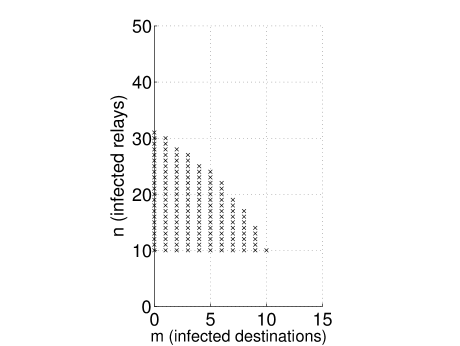
Figure 2: An illustration of the optimal policy. The symbols ’X’ mark the states in which the optimal action (at meeting with a relay) is to copy

IV Asymptotically Optimal Epidemic Forwarding

In states $[M_{\alpha}-1]\times[N_{0}:N]\times\{r\}$, the optimal action, which is governed by the function $\Phi(m,n)$, requires perfect knowledge of the network state $(m,n)$. This may not be available to the decision maker due to intermittent connectivity. In this section, we derive an asymptotically optimal policy that does not require knowledge of network’s state but depends only on the time elapsed since the generation of the packet. Such a policy is implementable if the packet is time-stamped when generated and the nodes’ clocks are synchronized.

IV-A Asymptotic Deterministic Dynamics

Our analysis closely follows Darling [11]. It is straightforward to show that the equations that follow are the conditional expected drift rates of the optimally controlled CTMC. For $(m(t),n(t))\in[M-1]\times[N_{0}:N]$, using the optimal policy in Theorem III.1, we get

$$\frac{{\rm d}\mathbb{E}(m(t)|(m(t),n(t)))}{{\rm d}t}= ~{}\lambda(m(t)+n(t))(M-m(t)),$$ (5a)

$$\frac{{\rm d}\mathbb{E}(n(t)|(m(t),n(t)))}{{\rm d}t}= ~{}\lambda(m(t)+n(t))(N-n(t))$$

$$\ \ \ \ \ \ \ \ \ \ \ \ \ 1_{\{\Phi(m(t),n(t))>0\}}.$$ (5b)

Recalling that $K=M+N$, the total number of nodes, we study large $K$ asymptotics. Towards this, we consider a sequence of problems indexed by $K$. The parameters of the $K$th problem are denoted using the superscript $K$. Normalized versions of these parameters, and normalized versions of the system state are denoted as follows:

$$\left.\begin{aligned} X=\frac{M^{K}}{K},~{}Y=\frac{N^{K}}{K},\\ X_{\alpha}=\frac{\alpha M^{K}}{K},~{}Y_{0}=\frac{N_{0}^{K}}{K},\\ \lambda^{K}=\frac{\Lambda}{K},\gamma^{K}=\frac{\Gamma}{K},\\ ~{}x^{K}(t)=\frac{m(t)}{K}\mbox{ and }y^{K}(t)=\frac{n(t)}{K}.\end{aligned}\right\}$$ (6)

Remarks IV.1

The pairwise meeting rate and the copying cost must both scale down as $K$ increases. Otherwise, the delivery delay will be negligible and the total transmission cost will be enormous for any policy, and no meaningful analysis is possible.

For each $K$, we define scaled two-dimensional integer lattice

$$\Delta^{K}=\left\{\left(\frac{i}{K},\frac{j}{K}\right):(i,j)\in[M^{K}-1]\times[N_{0}^{K}:N^{K}]\right\}.$$

$(x^{K}(t),y^{K}(t))\in\Delta^{K}$. Also, for $(x^{K}(t),y^{K}(t))\in\Delta^{K}$, using the notation in (6), the drift rates in (5a)-(5b) can be rewritten as follows.

$$\frac{{\rm d}\mathbb{E}(x^{K}(t)|(x^{K}(t),y^{K}(t)))}{{\rm d}t}$$

$$\ \ \ \ \ \ \ \ \ \ \ \ \ \ \ \ \ \ \ \ \ \ \ =f^{K}_{1}(x^{K}(t),y^{K}(t))$$

$$\ \ \ \ \ \ \ \ \ \ \ \ \ \ \ \ \ \ \ \ \ \ :=\Lambda(x^{K}(t)+y^{K}(t))(X-x^{K}(t)),$$ (7a)

$$\frac{{\rm d}\mathbb{E}(y^{K}(t)|(x^{K}(t),y^{K}(t)))}{{\rm d}t}$$

$$\ =f^{K}_{2}(x^{K}(t),y^{K}(t))$$

$$:=\Lambda(x^{K}(t)+y^{K}(t))(Y-y^{K}(t))1_{\{\phi^{K}(x^{K}(t),y^{K}(t))>0\}},$$ (7b)

where, for $(x,y)\in\Delta^{K}$,

$$\phi^{K}(x,y):=\sum_{j=Kx}^{\lceil KX_{\alpha}\rceil-1}\frac{1}{K\Lambda(y+\frac{j}{K})(y+\frac{j+1}{K})(X-\frac{j}{K})}-\Gamma.$$ (8)

We also define $(x(t),y(t))\in[0,X]\times[Y_{0},Y]$ as functions satisfying the following ODEs: $x(0)=0,y(0)=Y_{0}$, and for $t\geq 0$,

$$\frac{{\rm d}x(t)}{{\rm d}t}= ~{}f_{1}(x(t),y(t)):=\Lambda(x(t)+y(t))(X-x(t)),$$ (9a)

$$\frac{{\rm d}y(t)}{{\rm d}t}= ~{}f_{2}(x(t),y(t)):=\Lambda(x(t)+y(t))(Y-y(t))$$

$$\ \ \ \ \ \ \ \ \ \ \ \ \ \ \ \ \ \ \ \ \ \ \ \ \ \ \ \ \ \ \ 1_{\{\phi(x(t),y(t))>0\}}$$ (9b)

where

$$\phi(x,y)=\int_{z=x}^{X_{\alpha}}\frac{{\rm d}z}{\Lambda(y+z)^{2}(X-z)}-\Gamma.$$ (10)

Finally, we redefine the delivery delay $\mathcal{T}_{d}$ (see (1)) to be

$$\tau^{K} =\inf\{t\geq 0:x^{K}(t)\geq X_{\alpha}\},$$ (11)

$$\mbox{and }\tau =\inf\{t\geq 0:x(t)\geq X_{\alpha}\}.$$ (12)

Note that $\tau^{K}$ is a stopping time for the random process $(x^{K}(t),y^{K}(t))$, whereas $\tau$ is a deterministic time instant. Since $f^{K}_{1}(x,y)$ is bounded away from zero, $\tau^{K}<\infty$ with probability $1$. Similarly, on account of $f_{1}(x,y)$ being bounded away from zero, $\tau<\infty$.

Kurtz [10] and Darling [11] studied convergence of CTMCs to the solutions of ODEs. The following are the hypotheses for the version of the limit theorem that appears in Darling [11].

1. $\lim_{K\rightarrow\infty}\mathbb{P}\left(\|(x^{K}(0),y^{K}(0)-(x(0),y(0))\|>\epsilon\right)=0$;

2. In the scaled process $(x^{K}(t),y^{K}(t)$, the jump rates are $O(K)$ and drifts are $O(K^{-1})$;

3. $(f^{K}_{1}(x,y),f^{K}_{2}(x,y))$ converges to $(f_{1}(x,y),f_{2}(x,y))$ uniformly in $(x,y)$;

4. $(f_{1}(x,y),f_{2}(x,y))$ is Lipschitz continuous.

Observe that, in our case, only the first two hypotheses are satisfied. In particular, $f^{K}_{2}(x,y)$ does not converge uniformly to $f_{2}(x,y)$, and $f_{2}(x,y)$ is not Lipschitz over $[0,X_{\alpha}]\times[Y_{0},Y]$. Hence, the convergence results do not directly apply in our context. Thankfully, there is some regularity we can exploit which we now summarize as easily checkable facts.

1. $\phi^{K}(x,y)$ converges uniformly to $\phi(x,y)$;

2. the drift rates $f_{1}(x,y)$ and $f_{2}(x,y)$ are bounded from below and above;

3. $f_{1}(x,y)$ is Lipschitz and $f_{2}(x,y)$ is locally Lipschitz; and

4. for all small enough $\nu\in\mathbb{R}$, and all $(x,y)$ on the graph of “$\phi(x,y)=\nu$”, the direction in which the ODE progresses, $(f_{1}(x,y),f_{2}(x,y))$, is not tangent to the graph.

We then prove the following result which is identical to  [11, Theorem 2.8].

Theorem IV.1

Assume that $\alpha<1$ and $Y_{0}>0$. Then, for every $\epsilon,\delta>0$,

$$\lim_{K\rightarrow\infty}\mathbb{P}\left(\sup_{0\leq t\leq\tau}\|(x^{K}(t),y^{K}(t)-(x(t),y(t))\|>\epsilon\right)=0,$$

$$\lim_{K\rightarrow\infty}\mathbb{P}\left(|\tau^{K}-\tau|>\delta\right)=0.$$

Proof:

See Appendix B. ∎

We illustrate Theorem IV.1 using an example. Let $X=0.2,Y=0.8,\alpha=0.8,Y_{0}=0.2,\Lambda=0.05$ and $\Gamma=50$. In Figure 3, we plot $(x(t),y(t))$ and sample trajectories of $(x^{K}(t),y^{K}(t))$ for $K=100,200$ and $500$. We indicate the states at which the optimal policy stops copying to relays, i.e., $\Phi^{K}(x^{K}(t),y^{K}(t))$ goes below $0$ (see Theorem III.1) and the states at which the fraction of infected destinations crosses $X_{\alpha}$. We also show the corresponding states in the fluid model. The plots show that for large $K$, the fluid model captures the random dynamics of the network very well.

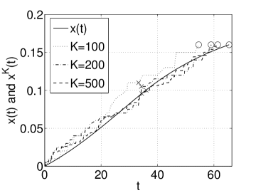
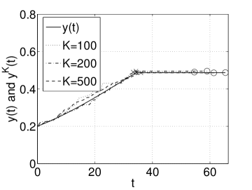
Figure 3: Simulation results: The top and bottom sub-plots respectively show the fractions of infected destinations and relays as a function of time. $(x^{K}(t),y^{K}(t))$ are obtained from a simulation of the controlled CTMC, and $(x(t),y(t))$ from the ODEs. The marker ’X’ indicates the states at which copying to relays is stopped whereas ’O’ indicates the states at which a fraction $\alpha$ of destinations have the packet.

IV-B Asymptotically Optimal Policy

Observe that $\phi(x,y)$ is decreasing in $x$ and $y$, both of which are nondecreasing with $t$. Consequently $\phi(x(t),y(t))$ decreases with $t$. We define

$$\tau^{\ast}:=\inf\{t\geq 0:\phi(x(t),y(t))\leq 0\}.$$ (13)

The limiting deterministic dynamics suggests the following policy $u^{\infty}$ for the original forwarding problem.

$$u^{\infty}(m,n,e)=\begin{cases}1\mbox{ if }e=d,\\ 1\mbox{ if }e=r\mbox{ and }t\leq\tau^{\ast},\\ 0\mbox{ if }e=r\mbox{ and }t>\tau^{\ast}.\end{cases}$$

We show that the policy $u^{\infty}$ is asymptotically optimal in the sense that its expected cost approaches the expected cost of the optimal policy $u^{\ast}$ as the network grows. Let us restate (IV-B) as

$$\mathbb{E}^{K}_{\pi}\{\mathcal{T}_{d}+\gamma\mathcal{E}_{c}\}= ~{}\frac{1}{K\Lambda Y_{0}(1-Y_{0})}+\left(\frac{Y-Y_{0}}{1-Y_{0}}\right.$$

$$~{}\left.J_{\pi}(0,Y_{0},r)+\frac{X}{1-Y_{0}}J_{\pi}(0,Y_{0},d)\right).$$

We have used superscript $K$ to show the dependence of cost on the network size. We then establish the following asymptotically optimality result.

Theorem IV.2

$$\lim_{K\rightarrow\infty}\mathbb{E}^{K}_{u^{\ast}}\{\mathcal{T}_{d}+\gamma\mathcal{E}_{c}\}=\lim_{K\rightarrow\infty}\mathbb{E}^{K}_{u^{\infty}}\{\mathcal{T}_{d}+\gamma\mathcal{E}_{c}\}=\tau+\Gamma y(\tau^{\ast}).$$

Proof:

See Appendix C. ∎

Remarks IV.2

Observe that we do not compare the limiting value of the optimal costs with the optimal cost on the (limiting) deterministic system. In general, these two may differ. However, the deterministic policy $u^{\infty}$ can be applied on the finite $K$-node system. The content of the above theorem is that given any $\epsilon>0$, cost of the policy $u^{\infty}$ is within $\epsilon$ of the optimal cost on the $K$-node system for all sufficiently large $K$.

Distributed Implementation

The asymptotically optimal policy can be implemented in a distributed fashion. Assume that all the nodes are time synchronized. Suppose that the packet is generated at the source at time $t_{0}$ (we assumed $t_{0}=0$ for the purpose of analysis). Given the system parameters $M,N,\alpha,N_{0},\lambda$ and $\gamma$, the source first extracts $X,Y,X_{\alpha},Y_{0},\Lambda$ and $\Gamma$ as in (6). Then, it calculates $\tau^{\ast}$ (see (13)), and stores $t_{0}+\tau^{\ast}$ as a header in the packet.

The packet is immediately copied to $N_{0}$ relays, perhaps by means of a broadcast from an infrastructure ”base station”. When an infected node meets a susceptible relay, it compares $t_{0}+\tau^{\ast}$ with the current time. The susceptible relay is not copied to if the current time exceeds $t_{0}+\tau^{\ast}$. However, all the infected nodes continue to carry the packet, and to copy to susceptible destinations as and when they meet.

Remarks IV.3

Consider a scenario, where the interest is in copying packet to only a fraction $\alpha$ of the destinations. Observe that for every $\epsilon>0$,

$$\lim_{K\rightarrow\infty}\mathbb{P}\left(\left|\frac{m(\tau)}{M}-\alpha\right|>\epsilon\right)=0.$$

Thus, in large networks, copying to destinations can also be stopped at time $\tau$ (see (12)) while ensuring that with large probability the fraction of infected destinations is close to $\alpha$. Consequently, all the relays can delete the packet and free their memory at $\tau$. This helps when packets are large and relay (cache) memory is limited.

V Optimal Two-Hop Forwarding

Instead of epidemic relaying one can consider two-hop relaying [17]. Here, the $N_{0}$ source nodes can copy the packet to any of the $N-N_{0}$ relays or $M$ destinations. The infected destinations can also copy the packet to any of the susceptible relays or destinations. However, the relays are allowed to transmit the packet only to the destinations. Here also a similar optimization problem as in Section II-A arises.

Now, the decision epochs $t_{k},k=1,2,\dots$ are the meeting epochs of the infected nodes (sources, relays or destinations) with the susceptible destinations and the meeting epochs of the sources or infected destinations with the susceptible relays. We can formulate an MDP with state

$$s_{k}:=(m_{k},n_{k},e_{k}).$$

at instant $t_{k}$ where $m_{k},n_{k}$ and $e_{k}$ are as defined in Section III-A. The state space is $[M_{\alpha}-1]\times[N_{0}:N]\times\mathcal{E}$. The control space is $\mathcal{U}\in\{0,1\}$, where $1$ is for copy and $0$ is for do not copy. We also get a transition structure identical to that in Section III-A.

For a state action pair $(s_{k},u_{k})$ the expected single stage cost is given by

$$g(s_{k},u_{k}) =\gamma u_{k}+\mathbb{E}\left\{\delta_{k+1}1_{\{m_{k+1}<M_{\alpha}\}}\right\}$$

$$=\begin{cases}\gamma u_{k}\mbox{ if }s_{k}\mbox{ is such that }m_{k}\geq M_{\alpha}\\ \gamma\mbox{ if }s_{k}=(M_{\alpha}-1,n,d)\mbox{ and }u_{k}=1\\ \gamma u_{k}+C_{d}(s_{k},u_{k})\mbox{ otherwise},\end{cases}$$

where
$C_{d}(s_{k},u_{k})=$

$$\ \ \ \ \ \frac{1}{\begin{split}\big{(}&(m_{k}+n_{k}+u_{k})(M-m_{k}-u_{k}1_{\{s_{k}=d\}})\lambda\\ &+(m_{k}+u_{k}1_{\{s_{k}=d\}}+N_{0})(N-n_{k}-u_{k}1_{\{s_{k}=r\}})\lambda\big{)}\end{split}}$$

is the mean time until the next decision epoch. As before, the quantity $\gamma u_{k}$ accounts for the transmission energy.

Let $u^{\ast}:[M_{\alpha}-1]\times[N_{0}:N]\times\mathcal{E}\rightarrow\mathcal{U}$ be a stationary optimal policy. As in Section III-B, the optimal policy satisfies $u^{\ast}(m,n,d)=1$ for all $(m,n)\in[M-1]\times[N_{0}:N]$, and $u^{\ast}(m,n,r)=0$ for all $(m,n)\in[M_{\alpha}:M-1]\times[N_{0}:N]$. Thus, we focus on a reduced state space $[M_{\alpha}-1]\times[N_{0}:N]\times\{r\}$. As before, we look for the one step look ahead policy which turns out to be the same as that for epidemic relaying. Finally, Theorem III.1 holds for two-hop relaying as well (see the proof in Appendix A).

Next, we turn to the asymptotically optimal control for two-hop relaying. The following are the conditional expected drift rates. For $(m(t),n(t))\in[M_{\alpha}-1]\times[N_{0}:N]$,

$$\frac{{\rm d}\mathbb{E}(m(t)|(m(t),n(t)))}{{\rm d}t}= ~{}\lambda(m(t)+n(t))(M-m(t)),$$

$$\frac{{\rm d}\mathbb{E}(n(t)|(m(t),n(t)))}{{\rm d}t}= ~{}\lambda(m(t)+N_{0})(N-n(t))$$

$$\ \ \ \ \ \ \ \ \ \ \ \ \ \ \ \ \ \ 1_{\{\Phi(m(t),n(t))>0\}}.$$

We employ the same scaling and notations as in (6). The drift rates in terms of $(x^{K}(t),y^{K}(t))\in[0,X_{\alpha}]\times[Y_{0},Y]$ are

$$\frac{{\rm d}\mathbb{E}(x^{K}(t)|(x^{K}(t),y^{K}(t)))}{{\rm d}t} =f^{K}_{1}(x^{K}(t),y^{K}(t))$$

$$:= ~{}\Lambda(x^{K}(t)+y^{K}(t))(X-x^{K}(t)),$$

$$\frac{{\rm d}\mathbb{E}(y^{K}(t)|(x^{K}(t),y^{K}(t)))}{{\rm d}t} =f^{K}_{2}(x^{K}(t),y^{K}(t))$$

$$:=\Lambda(x^{K}(t)+Y_{0}) (Y-y^{K}(t))1_{\{\phi^{K}(x^{K}(t),y^{K}(t))>0\}},$$

Now, $x(t),y(t)$ are defined as functions satisfying $x(0)=0,y(0)=Y_{0}$ and for $t\geq 0$,

$$\frac{{\rm d}x(t)}{{\rm d}t}= ~{}f_{1}(x(t),y(t)):=\Lambda(x(t)+y(t))(X-x(t)),$$

$$\frac{{\rm d}y(t)}{{\rm d}t}= ~{}f_{2}(x(t),y(t)):=\Lambda(x(t)+Y_{0})(Y-y(t))$$

$$\ \ \ \ \ \ \ \ \ \ \ \ \ \ \ \ \ \ \ \ \ \ \ \ \ \ \ \ \ \ \ \ \ \ \ \ \ \ \ 1_{\{\phi(x(t),y(t))>0\}}$$

The analysis in Section IV applies to two-hop relaying as well. In particular, Theorems IV.1 and IV.2 hold. However, for the identical system parameters ($M,N,\alpha,\lambda$ and $\gamma$) and initial state ($N_{0}$), the value of the time-threshold $\tau^{\ast}$ will be larger on account of the slower rates of infection of relays and destinations.

We illustrate the comparison between epidemic and two-hop relaying using an example. Let $X=0.2,Y=0.8,\alpha=0.8,Y_{0}=0.2,\Lambda=0.05$ and $\Gamma=50$. In Figure 4, we plot the graph of “$\phi(x,y)=0$”, and also the ’$y$ versus $x$’ trajectories corresponding to epidemic and two-hop relayings. In Figure 5, we plot the trajectories of $(x(t),y(t))$ corresponding to epidemic and two-hop relayings. As anticipated, the value of the time-threshold $\tau^{\ast}$ is larger for two-hop relaying than epidemic relaying. Moreover, the number of transmissions is less while the deliverly delay is more under the controlled two-hop relaying.

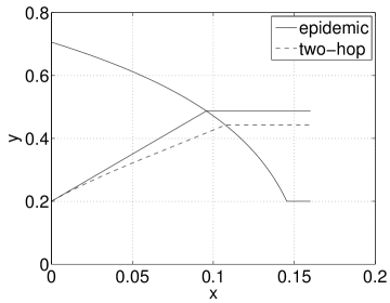
Figure 4: An illustration of the epidemic and two hop trajectories. The plots also show the graph of ‘$\phi(x,y)=0$’.

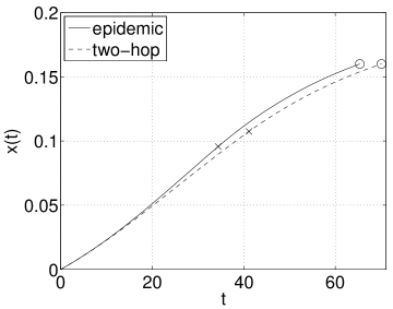
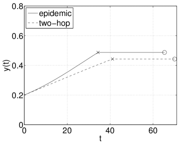
Figure 5: The top and bottom sub-plots respectively show the fractions of infected destinations and relays as a function of time. The marker ’X’ indicates the states at which copying to relays is stopped, and ’O’ indicates the states at which $\alpha$ fraction of destinations have been copied.

VI Numerical Results

We now show some numerical results to demonstrate the good performance of the deterministic control in epidemic forwarding in a DTN with multiple destinations. Let $X=0.2,Y=0.8,\alpha=0.8,Y_{0}=0.2$ and $\gamma=0.5$. We vary $\lambda$ from $0.00005$ to $0.05$ and use $K=50,100$ and $200$. In Figure 6, we plot the total number of copies to relays and the delivery delays corresponding to both the optimal and the asymptotically optimal deterministic policies. Evidently, the deterministic policy performs close to the optimal policy on both the fronts. We observe that, for a fixed $K$, both the mean delivery delay and the mean number of copies to relays decrease as $\lambda$ increases. We also observe that, for a fixed $\lambda$, the mean delivery delay decreases as the network size grows. Finally, for smaller values of $\lambda$, the mean number of copies to relays increases with the network size, and for larger values of $\lambda$, the opposite happens.

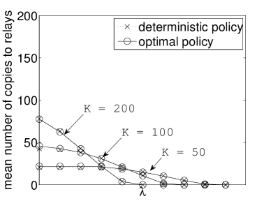
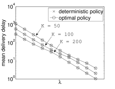
Figure 6: The top and bottom sub-plots, respectively, show the total number of copies to relays and the delivery delays corresponding to both the optimal and the deterministic policies.

VII Conclusion

We studied the epidemic forwarding in DTNs, formulated the problem as a controlled continuous time Markov chain, and obtained the optimal policy (Theorem III.1). We then developed an ordinary differential equation approximation for the optimally controlled Markov chain, under a natural scaling, as the population of nodes increases to $\infty$ (Theorem IV.1). This o.d.e. approximation yielded a forwarding policy that does not require global state information (and, hence, is implementable), and is asymptotically optimal (Theorem IV.2).

The optimal forwarding problem can also be addressed following the result of Gast et al. [14]. They study a general discrete time Markov decision process (MDP) [15]. However, they do not solve the finite problem citing the difficulties associated with obtaining the asymptotics of the optimally controlled process (see [14, Section 3.3]). Instead, they consider the fluid limit of the MDP, and analyze optimal control over the deterministic limiting problem. They then show that the optimal reward of the MDP converges to the optimal reward of its mean field approximation, given by the solution to a Hamilton-Jacobi-Bellman (HJB) equation [18, Section 3.2]. On the other hand, our approach is more direct. We have a continuous time controlled Markov chain at our disposal We explicitly characterize the optimal policy for the finite (complete information) problem, and prove convergence of the optimally controlled Markov chain to a fluid limit. An asymptotically optimal deterministic control is then suggested by the limiting deterministic dynamics, and does not require solving HJB equations. Our notion of asymptotic optimality is also stronger in the sense that we apply both the optimal policy and the deterministic policy to the finite problem, and show that the corresponding costs converge.

There are several directions in which this work can be extended. In the same DTN framework, there could be a deadline on the delivery time of the packet (or message); the goal of the optimal control could be to maximize the fraction of destinations that receive the packet before the deadline subject to an energy constraint. Our work in this paper assumes that network parameters such as $M,N,\lambda$ etc., are known; it will be important to address the adaptive control problem when these parameters are unknown.

Appendix A Proof of Theorem III.1

We first prove that for the optimal policy it is sufficient to consider two actions $1$ (i.e., copy now) and stop (i.e., do not copy now and never copy again). More precisely, under the optimal policy, if a susceptible relay that is met is not copied, then no susceptible relay is copied in the future as well. Let us fix a $N_{0}\leq n\leq N-1$. Let $m^{\ast}_{n}$ be the maximum $j$ such that $u^{\ast}(j,n,r)=1$. We show that $u^{\ast}(j,n,r)=1$ for all $0\leq j<m^{\ast}_{n}$; see Figure 2 for an illustration of this fact. The proof is via induction.

Proposition A.1

If $u^{\ast}(j,n,r)=1$ for all $m+1\leq j\leq m^{\ast}_{n}$, then $u^{\ast}(m,n,r)=1$.

Proof:

Define

$$\psi(m,n):= ~{}J_{0s}(m,n,r)-J(m,n,r),$$

$$\theta_{0}(m,n):= ~{}J_{0s}(m,n,r)-A((m,n,r),0),$$

$$\mbox{and }\theta_{1}(m,n):= ~{}J_{1s}(m,n,r)-A((m,n,r),1).$$

Both the action sequences that give rise to the two cost terms in the definition of $\theta_{0}(m,n)$, do not copy to the susceptible relay that was just met. Let $j$ be the number of infected destinations at the next decision epoch when a susceptible relay is met; $j$ can be $m,m+1,...,M$. All interim decision epochs must be meetings with susceptible destinations, and both policies copy at these meetings. Hence, both policies incur the same cost until this epoch, and differ by $\psi(j,n)$ in the costs to go (from this epoch onwards). Averaging the difference over $j$, and noting that $\psi(j,n)=0$ for $j>M_{\alpha}-1$, we get

$$\theta_{0}(m,n)=\sum_{j=m}^{M_{\alpha}-1}\left(\prod_{l=m}^{j-1}p_{l,n}(d)\right)p_{j,n}(r)\psi(j,n).$$ (14)

Since $A((m,n,r),0)\geq J(m,n,r)$, it follows that $\psi(m,n)\geq\theta_{0}(m,n)$, and so

$$\psi(m,n)\geq \sum_{j=m}^{M_{\alpha}-1}\left(\prod_{l=m}^{j-1}p_{l,n}(d)\right)p_{j,n}(r)\psi(j,n)$$

$$= \ p_{m,n}(r)\psi(m,n)$$

$$+p_{m,n}(d)\sum_{j=m+1}^{M_{\alpha}-1}\left(\prod_{l=m+1}^{j-1}p_{l,n}(d)\right)p_{j,n}(r)\psi(j,n)$$

which implies upon rearrangement

$$\psi(m,n)\geq\sum_{j=m+1}^{M_{\alpha}-1}\left(\prod_{l=m+1}^{j-1}p_{l,n}(d)\right)p_{j,n}(r)\psi(j,n)$$ (15)

Next, we establish the following lemma.

Lemma A.1

$\theta_{1}(m,n)\geq\theta_{1}(m+1,n).$

Proof:

Note that both the action sequences that lead to the two cost terms in the definition of $\theta_{1}(m,n)$ copy at state $(m,n,r)$. Subsequently, both incur equal costs until a decision epoch when an infected node meets a susceptible relay. Also, at any such state $(j,n+1,r),~{}j\geq m$, the costs to go differ by $\psi(j,n+1)$. Hence,

$$\theta_{1}(m,n) =\sum_{j=m}^{M_{\alpha}-1}\left(\prod_{l=m}^{j-1}p_{l,n+1}(d)\right)p_{j,n+1}(r)\psi(j,n+1)$$

$$=p_{m,n+1}(r)\psi(m,n+1)+p_{m,n+1}(d)\theta_{1}(m+1,n)$$

where

$$\theta_{1}(m+1,n)=\sum_{j=m+1}^{M_{\alpha}-1}\left(\prod_{l=m+1}^{j-1}p_{l,n+1}(d)\right)p_{j,n+1}(r)\psi(j,n+1).$$

Thus it suffices to show that

$$\psi(m,n+1)\geq\theta_{1}(m+1,n).$$

which is same as (15) with $n$ replaced by $n+1$. ∎

Next, observe that for all $m\leq j\leq m^{\ast}_{n}$,

$$\psi(j,n) ~{}=J_{0s}(j,n,r)-\min\{A((j,n,r),0),A((j,n,r),1)\}$$

$$~{}=\max\{\theta_{0}(j,n),\Phi(j,n)+\theta_{1}(j,n)\}.$$ (16)

Moreover, from the induction hypothesis, the optimal policy copies at states $(j,n,r)$ for all $m+1\leq j\leq m^{\ast}_{n}$. Hence, for $m+1\leq j\leq m^{\ast}_{n}$,

$$\psi(j,n)=\Phi(j,n)+\theta_{1}(j,n).$$

Finally, $\psi(j,n)=0$ for all $m^{\ast}_{n}<j\leq M_{\alpha}-1$ as the optimal policy does not copy in these states. Hence, from (14),

$$\theta_{0}(m,n)$$

$$~{}=p_{m,n}(r)\max\{\theta_{0}(m,n),\Phi(m,n)+\theta_{1}(m,n)\}+p_{m,n}(d)$$

$$\ \ \ \ \ \ \ \times\sum_{j=m+1}^{m^{\ast}_{n}}\left(\prod_{l=m+1}^{j-1}p_{l,n}(d)\right)p_{j,n}(r)\big{(}\Phi(j,n)+\theta_{1}(j,n)\big{)}$$

$$~{}<p_{m,n}(r)\max\left\{\theta_{0}(m,n),\Phi(m,n)+\theta_{1}(m,n)\right\}+p_{m,n}(d)$$

$$\ \ \ \ \times\big{(}\Phi(m,n)+\theta_{1}(m,n)\big{)}\sum_{j=m+1}^{m^{\ast}_{n}}\left(\prod_{l=m+1}^{j-1}p_{l,n}(d)\right)p_{j,n}(r)$$

$$~{}\leq p_{m,n}(r)\max\left\{\theta_{0}(m,n),\Phi(m,n)+\theta_{1}(m,n)\right\}$$

$$\ \ \ \ +p_{m,n}(d)\big{(}\Phi(m,n)+\theta_{1}(m,n)\big{)}$$

$$~{}=\max\left\{p_{m,n}(r)\theta_{0}(m,n)+p_{m,n}(d)\big{(}\Phi(m,n)+\theta_{1}(m,n)\big{)},\right.$$

$$\ \ \ \ \ \ \ \ \ \ \ \ \left.\Phi(m,n)+\theta_{1}(m,n)\right\},$$ (17)

where the first (strict) inequality holds because $\Phi(m,n)$ is strictly decreasing (see (4)) and $\theta_{1}(m,n)$ is decreasing (see Lemma A.1) in $m$ for fixed $n$. The second inequality follows because the summation term is a probability which is less than $1$. Now suppose that $\theta_{0}(m,n)\geq\Phi(m,n)+\theta_{1}(m,n)$. Then

$$\max\left\{p_{m,n}(r)\theta_{0}(m,n)+p_{m,n}(d)\big{(}\Phi(m,n)+\theta_{1}(m,n)\big{)},\right.$$

$$\ \ \ \ \ \ \ \ \left.\Phi(m,n)+\theta_{1}(m,n)\right\}$$

$$~{}=p_{m,n}(r)\theta_{0}(m,n)+p_{m,n}(d)\big{(}\Phi(m,n)+\theta_{1}(m,n)\big{)}$$

$$~{}\leq\theta_{0}(m,n)$$

which contradicts (17). Thus, we conclude that

$$\theta_{0}(m,n)<\Phi(m,n)+\theta_{1}(m,n).$$

This further implies that $\psi(m,n)=\Phi(m,n)+\theta_{1}(m,n)$ (see (16)), and so that $u^{\ast}(m,n,r)=1$. ∎

We now return to the proof of Theorem III.1. We show that the one-step look ahead policy is optimal for the resulting stopping problem. To see this, observe that $\Phi(m,n)$ is decreasing in $m$ for a given $n$ and also decreasing in $n$ for a given $m$. Thus, if $(m,n,r)\in\mathcal{S_{S}}$, i.e, $\Phi(m,n)\leq 0$ (see (3)), and the susceptible relay that is met is copied, the next state $(m,n+1,r)$ also belongs to the stopping set $\mathcal{S_{S}}$. In other words, $\mathcal{S_{S}}$ is also an absorbing set [15, Section 3.4]). Consequently, the one-step look ahead policy is an optimal policy.

Appendix B Proof of Theorem IV.1

We start with a preliminary result and a few definitions.

Proposition B.1

Let $\alpha<1$ and $Y_{0}>0$. Let $\phi^{K}$ and $\phi$ be as given in (8) and (10), respectively. Then, the functions $\phi^{K}(\cdot)$ converge to $\phi(\cdot)$ uniformly, i.e., for every $\nu>0$, there exists a $K_{\nu}$ such that

$$\sup_{(x,y)\in\Delta^{K}}|\phi^{K}(x,y)-\phi(x,y)|<\nu$$

for all $K\geq K_{\nu}$.

Proof:

For a $y\in[Y_{0},Y]$, define $f_{y}:[0,X_{\alpha}]\rightarrow\mathbb{R}_{+}$ as follows.

$$f_{y}(z)=\frac{1}{(y+z)^{2}(X-z)}.$$

Clearly, the family $\{f_{y}\}$ is positive and uniformly upper bounded. Indeed,

$$f_{y}(z)\leq f_{\max}:=\frac{1}{Y_{0}^{2}(X-X_{\alpha})}.$$

Further,

$$\frac{{\rm d}f_{y}(z)}{{\rm d}z}=\frac{1}{(y+z)^{2}(X-z)}\left(\frac{1}{X-z}-\frac{2}{y+z}\right),$$

from which it can be seen that

$$\left|\frac{{\rm d}f_{y}(z)}{{\rm d}z}\right|\leq f^{\prime}_{\max}$$

where $f^{\prime}_{\max}$ is a suitably defined constant. So the family $\{f_{y}\}$ is uniformly Lipschitz. Now, for $(z,y)\in[0,X_{\alpha}]\times[Y_{0},Y]$,

$$\frac{1}{K(y+z)(y+z+\frac{1}{K})(X-z)}-\int_{z}^{z+\frac{1}{K}}f_{y}(v){\rm d}v$$

$$~{}\leq\frac{f_{y}(z)}{K}-\int_{z}^{z+\frac{1}{K}}f_{y}(v){\rm d}v$$

$$~{}\leq\int_{z}^{z+\frac{1}{K}}(f_{y}(z)-f_{y}(v)){\rm d}v$$

$$~{}\leq\frac{f^{\prime}_{\max}}{K^{2}}$$ (18)

where the first and the last inequalities follow from the definitions of $f_{y}(z)$ and $f^{\prime}_{\max}$ respectively. On the other hand,

$$\frac{1}{(y+z)(y+z+\frac{1}{K})(X-z)} ~{}=f_{y}(z)\frac{y+z}{y+z+\frac{1}{K}}$$

$$~{}\geq f_{y}(z)\frac{Y_{0}}{Y_{0}+\frac{1}{K}}.$$

Hence

$$\int_{z}^{z+\frac{1}{K}}f_{y}(v){\rm d}v-\frac{1}{K(y+z)(y+z+\frac{1}{K})(X-z)}$$

$$~{}\leq\int_{z}^{z+\frac{1}{K}}f_{y}(v){\rm d}v-\frac{f_{y}(z)}{K}\frac{KY_{0}}{1+KY_{0}}$$

$$~{}\leq\int_{z}^{z+\frac{1}{K}}(f_{y}(v)-f_{y}(z)){\rm d}v+\frac{f_{y}(z)}{K(1+KY_{0})}$$

$$~{}\leq\frac{f^{\prime}_{\max}}{K^{2}}+\frac{f_{\max}}{K(1+KY_{0})}.$$ (19)

Combining (18) and (19),

$$\left|\frac{1}{K(y+z)(y+z+\frac{1}{K})(X-z)}-\int_{z}^{z+\frac{1}{K}}f_{y}(v){\rm d}v\right|$$

$$~{}\leq\frac{f^{\prime}_{\max}}{K^{2}}+\frac{f_{\max}}{K(1+KY_{0})}.$$

Now fix a $(x,y)\in\Delta^{K}$. Setting $z=j/K$, and summing over $j\in[Kx:\lceil KX_{\alpha}\rceil-1]$, we get

$$|\phi^{K}(x,y)-\phi(x,y)|$$

$$~{}\leq\sum_{j=Kx}^{\lceil KX_{\alpha}\rceil-1}\frac{1}{\Lambda}\left|\frac{1}{K(y+\frac{j}{K})(y+\frac{j+1}{K})(X-\frac{j}{K})}\right.$$

$$~{}\ \ \ \ \ \ \ \ \ \ \ \ \ \ \ \ \ \ \left.-\int_{\frac{j}{K}}^{\frac{j+1}{K}}f_{y}(v){\rm d}v\right|+\frac{1}{\Lambda}\left|\int_{\frac{\lceil KX_{\alpha}\rceil}{K}}^{X_{\alpha}}f_{y}(v)dv\right|$$

$$~{}\leq\frac{K(X_{\alpha}-x)}{\Lambda}\left(\frac{f^{\prime}_{\max}}{K^{2}}+\frac{f_{\max}}{K(1+KY_{0})}\right)+\frac{f_{\max}}{K\Lambda}$$

$$~{}\leq\frac{X_{\alpha}f^{\prime}_{\max}}{K\Lambda}+\frac{X_{\alpha}f_{\max}}{(1+KY_{0})\Lambda}+\frac{f_{\max}}{K\Lambda}.$$

The obtained upper bound on the right-hand side is independent of $(x,y)\in\Delta^{K}$, and vanishes as $K\rightarrow\infty$. Thus, for every $\nu>0$, there exists a $K_{\nu}$ such that

$$\sup_{(x,y)\in\Delta^{K}}|\phi^{K}(x,y)-\phi(x,y)|<\nu$$

for all $K\geq K_{\nu}$. ∎

In the following, to facilitate a parsimonious description, we use the notation $z^{K}(t)=(x^{K}(t),y^{K}(t))$, $z(t)=(x(t),y(t))$ and $\mathcal{Z}=[0,X_{\alpha}]\times[Y_{0},Y]$. Let us define, for a $\nu\in\mathbb{R}$,

$$\mathcal{S}_{\nu} ~{}=\{z\in\mathcal{Z}:\phi(z)>\nu\},$$

$$\tau_{\nu} ~{}=\inf\{t\geq 0:z(t)\notin\mathcal{S}_{\nu}\},$$

and a stopping time

$$\tau^{K}_{\nu}=\inf\{t\geq 0:z^{K}(t)\notin\mathcal{S}_{\nu}\},$$

the time when $z^{K}(t)$ exits the limiting set $\mathcal{S}_{\nu}$. Observe that

$$\frac{\partial\phi}{\partial x}=-\frac{1}{\Lambda(x+y)^{2}(X-x)}\leq-\frac{1}{\Lambda(X_{\alpha}+Y)^{2}X}$$ (20)

and $f^{K}_{1}(x,y)$ defined in (7a) is positive and is also bounded away from zero. These imply that $\tau^{K}_{\nu}<\infty$ with probability $1$. Similarly, $\tau_{\nu}<\infty$. The following assertion is a corollary of Proposition B.1.

Corollary B.1

Let $K_{\nu}$ be as in Proposition B.1. For $K\geq K_{\nu}$,

$$\phi^{K}(z)>0 ~{}\mbox{for all }z\in\mathcal{S}_{\nu},$$

$$\mbox{and }\phi^{K}(z)\leq 0 ~{}\mbox{for all }z\notin\mathcal{S}_{-\nu}.$$

We define the uncontrolled dynamics (i.e., the one in which the susceptible relays are always copied) as a Markov process $\bar{z}^{K}(t)=(\bar{x}^{K}(t),\bar{y}^{K}(t))$, $t\geq 0$ for which $\bar{z}^{K}(0)=z^{K}(0)$. Let $\bar{z}(t)=(\bar{x}(t),\bar{y}(t))$, $t\geq 0$ be the corresponding limiting deterministic dynamics. Formally, $\bar{z}(0)=z(0)$, and for $t\geq 0$,

$$\frac{{\rm d}\bar{x}(t)}{{\rm d}t}=\Lambda(\bar{x}(t)+\bar{y}(t))(X-\bar{x}(t)),$$

$$\frac{{\rm d}\bar{y}(t)}{{\rm d}t}=\Lambda(\bar{x}(t)+\bar{y}(t))(Y-\bar{y}(t)).$$

The quantities on the right-hand side of the above equations are at most $\Lambda$, and so

$$\left\|\frac{{\rm d}\bar{z}}{{\rm d}t}\right\|\leq\sqrt{2}\Lambda.$$

Also observe that the processes $\bar{z}^{K}(t)$ and $\bar{z}(t)$ satisfy the hypotheses of Darling [11] (see Section IV-A), and thus convergence of $\bar{z}^{K}(t)$ to $\bar{z}(t)$ follows.

We also define a Markov process $\tilde{z}^{K}(t)=(\tilde{x}^{K}(t),\tilde{y}^{K}(t))$, $t\geq\tau_{\nu}$ for which $\tilde{z}^{K}(\tau_{\nu})=z^{K}(\tau_{\nu})$ and

$$\frac{{\rm d}\mathbb{E}(\tilde{x}^{K}(t)|(\tilde{x}^{K}(t),\tilde{y}^{K}(t))}{{\rm d}t}= ~{}\Lambda(\tilde{x}^{K}(t)+\tilde{y}^{K}(t))(X-\bar{x}^{K}(t))$$

$$\frac{{\rm d}\mathbb{E}(y^{K}(t)|(x^{K}(t),y^{K}(t))}{{\rm d}t}= ~{}0$$

In other words, $\tilde{z}^{K}(t)$ is the process in which relays are not copied from $\tau_{\nu}$ onwards. Similarly, we define $\tilde{z}(t)=(\tilde{x}(t),\tilde{y}(t))$, $t\geq\tau_{\nu}$ as the solution of the corresponding differential equations. In other words, $\tilde{z}(\tau_{\nu})=z(\tau_{\nu})$, and for $t\geq\tau_{\nu}$,

$$\frac{{\rm d}\tilde{x}(t)}{{\rm d}t}= ~{}f_{1}(\tilde{x}(t),\tilde{y}(t)):=\Lambda(\tilde{x}(t)+\tilde{y}(t))(X-\tilde{x}(t)),$$

$$\frac{{\rm d}\tilde{y}(t)}{{\rm d}t}= ~{}f_{2}(\tilde{x}(t),\tilde{y}(t)):=0$$

We define

$$\tilde{\tau}^{K}_{-\nu} ~{}=\inf\{t\geq\tau_{\nu}:\tilde{z}^{K}(t)\notin\mathcal{S}_{-\nu}\},$$

$$\tilde{\tau}_{-\nu} ~{}=\inf\{t\geq\tau_{\nu}:\tilde{z}(t)\notin\mathcal{S}_{-\nu}\}.$$

Since

$$\Lambda Y_{0}(X-X_{\alpha})\leq\frac{{\rm d}\tilde{x}}{{\rm d}t}\leq\Lambda,$$

the lower bound implies that there is a strictly positive increase in $\tilde{x}$ after time $\tau_{\nu}$. Since $\Phi(x,y)$ decreases with increasing $x$ at a rate bounded away from $0$ (see 20), $\tilde{z}(t)$ must exit $S_{-\nu}$ within a short additional duration. Thus, we have that

$$\tilde{\tau}_{-\nu}-\tau_{\nu}\leq b\nu$$

for a suitably chosen $b<\infty$.

To aid the reader, we summarize the variables used in Table I. We also illustrate sample trajectories of a controlled CTMC and the corresponding ODE via an example (Figure 7). We choose $M=40,N=160,\alpha=0.8,N_{0}=40,\lambda=0.00025$ and $\gamma=0.25$. We plot the graphs of ’$\phi(x,y)=\nu$’ and ’$\phi(x,y)=-\nu$’ for $\nu=0.2$. We also show the trajectories “$y^{K}$ vs $x^{K}$”, “$y$ vs $x$”, “$\tilde{y}$ vs $\tilde{x}$” and the epochs $\tau_{\nu}$, $\tau_{-\nu}$ and $\tilde{\tau}_{-\nu}$.

TABLE I: Variables and their description

variables	description
$z^{K}(t)$	controlled dynamics with discontinuity at $\tau^{K}$
$z(t)$	$z^{K}(t)$’s fluid limit with discontinuity at $\tau^{\ast}$
$\tau^{K}_{\nu}$	instant when $z^{K}(t)$ exits $\mathcal{S}_{\nu}$
$\tau_{\nu}$	instant when $z(t)$ exits $\mathcal{S}_{\nu}$
$\bar{z}^{K}(t)$	uncontrolled dynamics with no discontinuity
$\bar{z}(t)$	$\bar{z}^{K}(t)$’s fluid limit with no discontinuity
$\tilde{z}^{K}(t)$	identical to $z^{K}(t)$ until $\tau_{\nu}$ at which copying to
	relays is stopped
$\tilde{z}(t)$	$\tilde{z}^{K}(t)$’s fluid limit with discontinuity at $\tau_{\nu}$
$\tilde{\tau}^{K}_{-\nu}$	instant when $\tilde{z}^{K}(t)$ exits $\mathcal{S}_{-\nu}$
$\tilde{\tau}_{-\nu}$	instant when $\tilde{z}(t)$ exits $\mathcal{S}_{-\nu}$

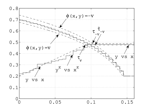
Figure 7: An illustration of the trajectories of the controlled CTMC and the corresponding ODE, and the associated variables.

We prove the assertion in Theorem IV.1 in three steps: (a) over $[0,\tau_{\nu}]$, (b) over $[\tau_{\nu},\tilde{\tau}_{-\nu}]$ and (c) over $[\tilde{\tau}_{-\nu},\tau]$. However, we also need the following lemmas in our proof..

Lemma B.1

For every $\epsilon>0$, there exists a $\bar{\tau}_{\epsilon}$ such that for all $t\geq 0$, $0\leq u\leq\bar{\tau}_{\epsilon}$,

$$\mathbb{P}\left(\|\bar{z}^{K}(t+u)-\bar{z}^{K}(t)\|>\epsilon\right)=O(K^{-1}).$$

Proof:

Observe that

$$\|\bar{z}^{K}(t+u)-\bar{z}^{K}(t)\|$$

$$~{}\leq\|\bar{z}^{K}(t)-\bar{z}(t)\|+\|\bar{z}^{K}(t+u)-\bar{z}(t+u)\|$$

$$~{}\ \ \ \ \ \ \ \ \ \ \ \ \ \ \ \ \ \ \ \ \ \ \ \ \ \ \ \ \ \ \ \ \ \ \ \ \ \ \ \ \ \ \ \ \ \ +\|\bar{z}(t)-\bar{z}(t+u)\|$$

$$~{}\leq\|\bar{z}^{K}(t)-\bar{z}(t)\|+\|\bar{z}^{K}(t+u)-\bar{z}(t+u)\|+\sqrt{2}\Lambda u$$

Hence, for all $t\geq 0$, $u\geq 0$,

$$\mathbb{P}\left(\|\bar{z}^{K}(t+u)-\bar{z}^{K}(t)\|>\sqrt{2}\Lambda u+\frac{\epsilon}{2}\right)$$

$$~{}\leq\mathbb{P}\left(\|\bar{z}^{K}(t)-\bar{z}(t)\|+\|\bar{z}^{K}(t+u)-\bar{z}(t+u)\|>\frac{\epsilon}{2}\right)$$

$$~{}\leq\mathbb{P}\left(\sup_{t\leq s\leq t+u}\|\bar{z}^{K}(s)-\bar{z}(s)\|>\frac{\epsilon}{4}\right)$$

$$~{}=O(K^{-1})$$

where the last equality follows from [11, Theorem 2.8]. Setting $\bar{\tau}_{\epsilon}=\frac{\epsilon}{2\sqrt{2}\Lambda}$, for all $t\geq 0$, $0\leq u\leq\bar{\tau}_{\epsilon}$

$$\mathbb{P}\left(\|\bar{z}^{K}(t+u)-\bar{z}^{K}(t)\|>\epsilon\right)$$

$$~{}\leq\mathbb{P}\left(\|\bar{z}^{K}(t+u)-\bar{z}^{K}(t)\|>\sqrt{2}\Lambda u+\frac{\epsilon}{2}\right)$$

$$~{}=O(K^{-1}).$$

∎

Lemma B.2

Suppose $u$ is a fixed time and $u^{K}$ is a random time that satisfies $\mathbb{P}\left(|u-u^{K}|>\delta\right)=O(K^{-1})$ for every $\delta>0$. Then, for every $\epsilon>0$,

$$\mathbb{P}\left(\|\bar{z}^{K}(u)-\bar{z}^{K}(u\wedge u^{K})\|>\epsilon\right)=O(K^{-1})$$

Proof:

Fix a $\delta>0$. Then,

$$\mathbb{P}(\|\bar{z}^{K}(u)-\bar{z}^{K}(u\wedge u^{K})\|>\epsilon)$$

$$=\mathbb{P}(u-u^{K}>\delta)$$

$$\ \ \ \ \ \ \ \ \ \ \ \ \ \ \ \ \mathbb{P}\left(\|\bar{z}^{K}(u)-\bar{z}^{K}(u\wedge u^{K})\|>\epsilon\big{|}u-u^{K}>\delta\right)$$

$$~{}\ \ +\mathbb{P}(u-u^{K}\leq\delta)$$

$$\ \ \ \ \ \ \ \ \ \ \ \ \ \ \ \ \mathbb{P}\left(\|\bar{z}^{K}(u)-\bar{z}^{K}(u\wedge u^{K})\|>\epsilon\big{|}u-u^{K}\leq\delta\right)$$

$$\leq O(K^{-1})+\mathbb{P}\left(\|\bar{z}^{K}(u)-\bar{z}^{K}(u\wedge u^{K})\|>\epsilon\big{|}u-u^{K}\leq\delta\right)$$

$$\leq O(K^{-1})+\mathbb{P}\left(\|\bar{z}^{K}(u)-\bar{z}^{K}(u-\delta)\|>\epsilon\big{|}u-u^{K}\leq\delta\right)$$

where the last inequality holds because $\bar{z}^{K}(t)$ is a monotone increasing function. Setting $\delta=\bar{\tau}_{\epsilon}$ (see Lemma B.1),

$$\mathbb{P}(\|\bar{z}^{K}(u)-\bar{z}^{K}(u\wedge u^{K})\|>\epsilon)$$

$$\leq O(K^{-1})+\mathbb{P}\left(\|\bar{z}^{K}(u)-\bar{z}^{K}(u-\bar{\tau}_{\epsilon})\|>\epsilon\big{|}u-u^{K}\leq\bar{\tau}_{\epsilon}\right)$$

$$=O(K^{-1})+\mathbb{P}\left(\|\bar{z}^{K}(u)-\bar{z}^{K}(u-\bar{\tau}_{\epsilon})\|>\epsilon\right)$$

$$\leq O(K^{-1})+O(K^{-1})$$

$$=O(K^{-1})$$

where the last inequality follows from Lemma B.1. ∎

Following is the proof of Theorem IV.1.

(a) First, we prove the convergence of $z^{K}(t)$ to $z(t)$ over $[0,\tau_{\nu}]$. Fix a $\nu>0$. Then Corollary B.1 implies that $z^{K}(t)$ converges to $z(t)$ in the region $\mathcal{S}_{\nu}$. Following [11, Theorem 2.8] we have, for all $\epsilon,\delta>0$, $\displaystyle\mathbb{P}\left(\sup_{0\leq t\leq\tau_{\nu}}\|z^{K}(t\wedge\tau^{K}_{\nu})-z(t)\|>\epsilon\right)=O(K^{-1})$ (21a) $\displaystyle\mbox{and }\mathbb{P}(|\tau^{K}_{\nu}-\tau_{\nu}|>\delta)=O(K^{-1}).$ (21b) Since, for all $t\geq 0$, $$\|z^{K}(t)-z(t)\|\leq\|z^{K}(t\wedge\tau^{K}_{\nu})-z(t)\|+\|z^{K}(t)-z^{K}(t\wedge\tau^{K}_{\nu})\|,$$ we obtain $\displaystyle\sup_{0\leq t\leq\tau_{\nu}}\|z^{K}(t)-z(t)\|\leq$ $\displaystyle~{}\sup_{0\leq t\leq\tau_{\nu}}\|z^{K}(t\wedge\tau^{K}_{\nu})-z(t)\|$ $\displaystyle~{}+\sup_{0\leq t\leq\tau_{\nu}}\|z^{K}(t)-z^{K}(t\wedge\tau^{K}_{\nu})\|.$ If the left side is larger than $\epsilon$, at least one of the two terms on the right side is larger than $\epsilon/2$, and so by the union bound, we get $\displaystyle\mathbb{P}\left(\sup_{0\leq t\leq\tau_{\nu}}\|z^{K}(t)-z(t)\|>\epsilon\right)$ $\displaystyle\leq\mathbb{P}\left(\sup_{0\leq t\leq\tau_{\nu}}\|z^{K}(t\wedge\tau^{K}_{\nu})-z(t)\|>\frac{\epsilon}{2}\right)$ $\displaystyle~{}\ \ +\mathbb{P}\left(\sup_{0\leq t\leq\tau_{\nu}}\|z^{K}(t)-z^{K}(t\wedge\tau^{K}_{\nu})\|>\frac{\epsilon}{2}\right)$ $\displaystyle\leq O(K^{-1})+\mathbb{P}\left(\|z^{K}(\tau_{\nu})-z^{K}(\tau_{\nu}\wedge\tau^{K}_{\nu})\|>\frac{\epsilon}{2}\right)$ (22) where the first term in the last inequality follows from (21a). Also, from corollary B.1, for $K\geq K_{\nu}$, $\phi^{K}(z^{K}(\tau^{K}_{\nu})-)>0$, i.e., the process $z^{K}(t)$ follows uncontrolled dynamics until $\tau^{K}_{\nu}$. Thus, for $K\geq K_{\nu}$, $z^{K}(\tau^{K}_{\nu})=\bar{z}^{K}(\tau^{K}_{\nu})$ and $$\|z^{K}(\tau_{\nu})-z^{K}(\tau_{\nu}\wedge\tau^{K}_{\nu})\|\leq\|\bar{z}^{K}(\tau_{\nu})-\bar{z}^{K}(\tau_{\nu}\wedge\tau^{K}_{\nu})\|$$ sample path wise. The inequality is an equality if $\tau_{\nu}\leq\tau_{\nu}^{K}$; both sides equal $0$ in this case. Otherwise, it is an inequality because the possible change in dynamics of $z^{K}(t)$ after $\tau^{K}_{\nu}$ makes it increase (in both its components) at a slower pace than the uncontrolled $\bar{z}^{K}(t)$. Thus $\displaystyle\mathbb{P}\left(\|z^{K}(\tau_{\nu})-z^{K}(\tau_{\nu}\wedge\tau^{K}_{\nu})\|>\frac{\epsilon}{2}\right)$ $\displaystyle~{}\leq\mathbb{P}\left(\|\bar{z}^{K}(\tau_{\nu})-\bar{z}^{K}(\tau_{\nu}\wedge\tau^{K}_{\nu})\|>\frac{\epsilon}{2}\right)$ $\displaystyle~{}\leq O(K^{-1})$ where the last inequality follows from (21b) and Lemma B.2. Using this in (22) we get $\displaystyle\mathbb{P}\left(\sup_{0\leq t\leq\tau_{\nu}}\|z^{K}(t)-z(t)\|>\epsilon\right)$ $\displaystyle~{}\leq O(K^{-1})+O(K^{-1})$ $\displaystyle~{}=O(K^{-1})$ (b) Now we prove the convergence of $z^{K}(t)$ to $z(t)$ over $[\tau_{\nu},\tilde{\tau}_{-\nu}]$. Observe that, for $t\in[\tau_{\nu},\tilde{\tau}_{-\nu}]$, $\displaystyle\|z^{K}(t)-z(t)\|$ $\displaystyle\leq\|z^{K}(\tau_{\nu})-z(\tau_{\nu})\|+\|z^{K}(t)-z^{K}(\tau_{\nu})\|+\|z(t)-z(\tau_{\nu})\|.$ Hence, $\displaystyle\sup_{\tau_{\nu}\leq t\leq\tilde{\tau}_{-\nu}}\|z^{K}(t)-z(t)\|$ $\displaystyle~{}\leq\|z^{K}(\tau_{\nu})-z(\tau_{\nu})\|+\sup_{\tau_{\nu}\leq t\leq\tilde{\tau}_{-\nu}}\|z^{K}(t)-z^{K}(\tau_{\nu})\|$ $\displaystyle~{}\ \ \ \ \ \ \ \ \ \ \ \ \ \ \ \ \ \ \ \ \ \ \ \ \ +\sup_{\tau_{\nu}\leq t\leq\tilde{\tau}_{-\nu}}\|z(t)-z(\tau_{\nu})\|$ $\displaystyle~{}=\|z^{K}(\tau_{\nu})-z(\tau_{\nu})\|+\|z^{K}(\tilde{\tau}_{-\nu})-z^{K}(\tau_{\nu})\|$ $\displaystyle~{}\ \ \ \ \ \ \ \ \ \ \ \ \ \ \ \ \ \ \ \ \ \ \ \ \ +\|z(\tilde{\tau}_{-\nu})-z(\tau_{\nu})\|$ $\displaystyle~{}\leq\|z^{K}(\tau_{\nu})-z(\tau_{\nu})\|+\|z^{K}(\tilde{\tau}_{-\nu})-z^{K}(\tau_{\nu})\|+\sqrt{2}\Lambda b\nu$ where the equality follows because the $z^{(}t)$ and $z(t)$ are nondecreasing. The last inequality holds because $\|{\rm d}{z}/{\rm d}t\|\leq\|{\rm d}{\bar{z}}/{\rm d}t\|\leq\sqrt{2}\Lambda$ and $\tilde{\tau}_{-\nu}-\tau_{\nu}\leq b\nu$. Moreover, $\displaystyle\mathbb{P}$ $\displaystyle\left(\sup_{\tau_{\nu}\leq t\leq\tilde{\tau}_{-\nu}}\|z^{K}(t)-z(t)\|>\sqrt{2}\Lambda b\nu+\frac{\epsilon}{2}\right)$ $\displaystyle~{}\leq\mathbb{P}\left(\|z^{K}(\tau_{\nu})-z(\tau_{\nu})\|>\frac{\epsilon}{4}\right)$ $\displaystyle~{}\ \ \ \ \ \ \ \ \ \ \ \ \ \ \ \ \ \ \ \ +\mathbb{P}\left(\|z^{K}(\tilde{\tau}_{-\nu})-z^{K}(\tau_{\nu})\|>\frac{\epsilon}{4}\right)$ $\displaystyle~{}=O(K^{-1})+\mathbb{P}\left(\|z^{K}(\tilde{\tau}_{-\nu})-z^{K}(\tau_{\nu})\|>\frac{\epsilon}{4}\right)$ where the equality follows from the result of part (a). We now redefine the Markov process $\bar{z}^{K}(t)=(\bar{x}^{K}(t),\bar{y}^{K}(t))$ for $t\geq\tau_{\nu}$, to be the uncontrolled dynamics with initial condition $\bar{z}^{K}(\tau_{\nu})=z^{K}(\tau_{\nu})$. Again, it can be easily observed that $$\|z^{K}(\tilde{\tau}_{-\nu})-z^{K}(\tau_{\nu})\|\leq\|\bar{z}^{K}(\tilde{\tau}_{-\nu})-\bar{z}^{K}(\tau_{\nu})\|.$$ Thus $\displaystyle\mathbb{P}$ $\displaystyle\left(\sup_{\tau_{\nu}\leq t\leq\tilde{\tau}_{-\nu}}\|z^{K}(t)-z(t)\|>\sqrt{2}\Lambda b\nu+\frac{\epsilon}{2}\right)$ $\displaystyle~{}\leq O(K^{-1})+\mathbb{P}\left(\|\bar{z}^{K}(\tilde{\tau}_{-\nu})-\bar{z}^{K}(\tau_{\nu})\|>\frac{\epsilon}{4}\right)$ $\displaystyle~{}\leq O(K^{-1})+\mathbb{P}\left(\|\bar{z}^{K}(\tau_{\nu}+b\nu)-\bar{z}^{K}(\tau_{\nu})\|>\frac{\epsilon}{4}\right)$ Set $\nu=\min\{\frac{\epsilon}{2\sqrt{2}\Lambda b},\bar{\tau}_{\frac{\epsilon}{4b}}\}$, and apply Lemma B.1 to get $\displaystyle\mathbb{P}\left(\sup_{\tau_{\nu}\leq t\leq\tilde{\tau}_{-\nu}}\|z^{K}(t)-z(t)\|>\epsilon\right)$ $\displaystyle~{}\leq\mathbb{P}\left(\sup_{\tau_{\nu}\leq t\leq\tilde{\tau}_{-\nu}}\|z^{K}(t)-z(t)\|>\sqrt{2}\Lambda b\nu+\frac{\epsilon}{2}\right)$ $\displaystyle~{}\leq O(K^{-1})+O(K^{-1})$ $\displaystyle~{}=O(K^{-1}).$ (c) Finally, we prove the convergence of $z^{K}(t)$ to $z(t)$ over $[\tilde{\tau}_{-\nu},\tau]$. Reconsider the process $\tilde{z}^{K}(t),t\geq\tau_{\nu}$ and the associated function $\tilde{z}(t)$. Recall that, for any $\nu>0$, $\tilde{z}^{K}(t)$ and $\tilde{z}(t)$ exit $\mathcal{S}_{-\nu}$ at $\tilde{\tau}^{K}_{-\nu}$ and $\tilde{\tau}_{-\nu}$ respectively. Clearly, $\tilde{\tau}_{-\nu/2}<\tilde{\tau}_{-\nu}$; say $\tilde{\tau}_{-\nu}-\tilde{\tau}_{-\nu/2}=\delta_{\nu}$. Also, using [11, Theorem 2.8], $\displaystyle~{}\mathbb{P}\left(\tilde{\tau}^{K}_{-\nu/2}-\tilde{\tau}_{-\nu/2}>\delta_{\nu}\right)=O(K^{-1})$ i.e., $\displaystyle~{}\mathbb{P}\left(\tilde{\tau}^{K}_{-\nu/2}>\tilde{\tau}_{-\nu}\right)=O(K^{-1})$ Furthermore, we have that $\tau^{K}_{-\nu/2}\leq\tilde{\tau}^{K}_{-\nu/2}$ sample path wise. The inequality holds because $z^{K}(t)$ may continue to increase (in both its components) at a higher pace than $\tilde{z}^{K}(t)$ even after $\tau_{\nu}$. Thus $$\mathbb{P}\left(\tau^{K}_{-\nu/2}>\tilde{\tau}_{-\nu}\right)=O(K^{-1}),$$ implying that the probability that $z^{K}(t)$ has changed its dynamics by $\tilde{\tau}_{-\nu}$ approaches $1$ as $K$ approaches $\infty$. In these realizations, the dynamics of $z^{K}(t)$ and $z(t)$ match for $t\geq\tilde{\tau}_{-\nu}$. We restrict ourselves to only these realizations. We also have from part (b) that, for every $\epsilon>0$, $$\mathbb{P}\left(\|z^{K}(\tilde{\tau}_{-\nu})-z(\tilde{\tau}_{-\nu})\|>\epsilon\right)=O(K^{-1})$$ Once more using [11, Theorem 2.8], for any $\epsilon,\delta>0$ $\displaystyle\mathbb{P}\left(\sup_{\tilde{\tau}_{-\nu}\leq t\leq\tau}\|z^{K}(t)-z(t)\|>\epsilon\right)=O(K^{-1})$ and $\displaystyle\mathbb{P}\left(|\tau^{K}-\tau|>\delta\right)=O(K^{-1}).$

Appendix C Proof of Theorem IV.2

For the optimal policy $u^{\ast}$, the total expected cost

$$\mathbb{E}^{K}_{u^{\ast}}\{\mathcal{T}_{d}+\gamma\mathcal{E}_{c}\}=\mathbb{E}^{K}_{u^{\ast}}\{\tau^{K}+\Gamma(X+y^{K}(\tau^{K}))\}$$

since $\mathcal{T}_{d}=\tau^{K}$ by definition (see (11)); we use the subscript $u^{\ast}$ to show dependence of the probability law on the underlying policy. Under the deterministic policy $u^{\infty}$, copying to relays is stopped at the deterministic time instant $\tau^{\ast}<\tau$, implying $y^{K}(\tau^{\ast})=y^{K}(\tau)$. Thus, the total expected cost

$$\mathbb{E}^{K}_{u^{\infty}}\{\mathcal{T}_{d}+\gamma\mathcal{E}_{c}\}=\mathbb{E}^{K}_{u^{\infty}}\{\tau^{K}+\Gamma(X+y^{K}(\tau))\}.$$

Also observe that for $(x^{K}(t),y^{K}(t))$ under $u^{\infty}$, the corresponding fluid limits are the same deterministic dynamics $(x(t),y(t))$ defined in Section IV-A (i.e., solutions of (9a)-(9b)). $(x^{K}(t),y^{K}(t))$ and $(x(t),y(t))$ satisfy the hypotheses assumed in Darling [11] over the intervals $[0,\tau^{\ast}]$ and $[\tau^{\ast},\infty)$. Thus [11, Theorem 2.8] applies, and we conclude 

$$\lim_{K\rightarrow\infty}\mathbb{P}^{K}_{u^{\infty}}\left(\sup_{0\leq t\leq\tau}\|(x^{K}(t),y^{K}(t))-(x(t),y(t))\|>\epsilon\right)=0,$$

$$\lim_{K\rightarrow\infty}\mathbb{P}^{K}_{u^{\infty}}\left(|\tau^{K}-\tau|>\delta\right)=0.$$

Furthermore, it can be easily shown that under both the controls $u^{\ast}$ and $u^{\infty}$, the delivery delays $\tau^{K}$ have second moments that are bounded uniformly over all $K$. To see this, consider a policy $u^{0}$ that never copies to relays. Clearly,

$$\mathbb{E}^{K}_{u^{\ast}}(\tau^{K})^{2}< \mathbb{E}^{K}_{u^{0}}(\tau^{K})^{2},$$

$$\mathbb{E}^{K}_{u^{\infty}}(\tau^{K})^{2}< \mathbb{E}^{K}_{u^{0}}(\tau^{K})^{2}$$

for each $K$. Then is suffices to show that

$$\sup_{K}\mathbb{E}^{K}_{u^{0}}(\tau^{K})^{2}<\infty.$$ (23)

Note that

$$\tau^{K}=\sum_{m=0}^{M^{K}_{\alpha}-1}\bar{\delta}_{m}$$

where $\bar{\delta}_{m}$ is the time duration for which $m(t)=m$; $\bar{\delta}_{m},m=0,1,\dots$ are independent, and $\bar{\delta}_{m}$ is exponentially distributed with mean $\frac{1}{\lambda^{K}(m+N^{K}_{0})(M^{K}-m)}$ under policy $u^{0}$. Thus

$$\mathbb{E}^{K}_{u^{0}}\tau^{K}= \sum_{m=0}^{M^{K}_{\alpha}-1}\frac{1}{\lambda^{K}(m+N^{K}_{0})(M^{K}-m)}$$

$$\leq \sum_{m=0}^{M^{K}_{\alpha}-1}\frac{1}{\lambda^{K}N^{K}_{0}(M^{K}-M^{K}_{\alpha})}$$

$$= \frac{M^{K}_{\alpha}}{\lambda^{K}N^{K}_{0}(M^{K}-M^{K}_{\alpha})}$$

$$= \frac{X_{\alpha}}{\Lambda Y_{0}(X-X_{\alpha})}$$

$$< \infty$$

Similarly,

$$\mbox{Var}^{K}_{u^{0}}\tau^{K}= \sum_{m=0}^{M^{K}_{\alpha}-1}\frac{1}{\left(\lambda^{K}(m+N^{K}_{0})(M^{K}-m)\right)^{2}}$$

$$\leq \frac{M^{K}_{\alpha}}{\left(\lambda^{K}N^{K}_{0}(M^{K}-M^{K}_{\alpha})\right)^{2}}$$

$$= \frac{X_{\alpha}}{K\Lambda^{2}Y^{2}_{0}(X-X_{\alpha})^{2}}$$

$$\rightarrow 0$$

as $K\rightarrow\infty$. These results together imply (23).

Following [19, Remark 9.5.1], under both $u^{\ast}$ and $u^{\infty}$, $\tau^{K}$ are uniformly integrable. Since, $\tau^{K}$, under both $u^{\ast}$ and $u^{\infty}$, converge to $\tau$ in probability and hence in distribution, [19, Theorem 9.5.1] yields

$$\lim_{K\rightarrow\infty}\mathbb{E}^{K}_{u^{\ast}}\tau^{K}=\lim_{K\rightarrow\infty}\mathbb{E}^{K}_{u^{\infty}}\tau^{K}=\tau.$$ (24)

Next, it is easy to show that under the control $u^{\ast}$, $y^{K}(\tau^{K})$ converges to $y(\tau)$ in probability. To see this, observe that

$$|y^{K}(\tau^{K})-y(\tau)|\leq|y^{K}(\tau^{K})-y^{K}(\tau)|+|y^{K}(\tau)-y(\tau)|.$$ (25)

From Theorem IV.1, $y^{K}(\tau)$ and $\tau^{K}$ converge to $y(\tau)$ and $\tau$ respectively, in probability. The latter result, along with the arguments similar to those in the proof of Lemma B.2, implies that

$$\mathbb{P}\left(|y^{K}(\tau^{K})-y^{K}(\tau)|>\epsilon\right)=O(K^{-1})$$

for every $\epsilon>0$. Using these facts in (25), we conclude that

$$\mathbb{P}\left(|y^{K}(\tau^{K})-y(\tau)|>\epsilon\right)=O(K^{-1}).$$

for every $\epsilon>0$. Since $y^{K}(\tau^{K})$ is bounded, and hence uniformly integrable, [19, Theorem 9.5.1] implies that

$$\lim_{K\rightarrow\infty}\mathbb{E}^{K}_{u^{\ast}}y^{K}(\tau^{K})=y(\tau).$$ (26)

Similarly, under the control $u^{\infty}$ also, $y^{K}(\tau)$ is bounded, and hence is uniformly integrable. It also converges to $y(\tau)$ in probability. Once more using [19, Theorem 9.5.1], we get

$$\lim_{K\rightarrow\infty}\mathbb{E}^{K}_{u^{\infty}}y^{K}(\tau)=y(\tau).$$ (27)

Combining (26) and (27)

$$\lim_{K\rightarrow\infty}\mathbb{E}^{K}_{u^{\ast}}y^{K}(\tau^{K})=\lim_{K\rightarrow\infty}\mathbb{E}^{K}_{u^{\infty}}y^{K}(\tau).$$ (28)

Finally, combining (24) and (28), we get that

$$\lim_{K\rightarrow\infty}\mathbb{E}^{K}_{u^{\ast}}\{\mathcal{T}_{d}+\gamma\mathcal{E}_{c}\}=\lim_{K\rightarrow\infty}\mathbb{E}^{K}_{u^{\infty}}\{\mathcal{T}_{d}+\gamma\mathcal{E}_{c}\}=\tau+\Gamma y(\tau^{\ast}).$$

Appendix D The Hamiltonian Formulation and The Solution

In this section we consider the limiting deterministic (fluid) system and study its optimal control. The limiting controlled system is: $x(0)=0$, $y(0)=Y_{0}$, and for $t\geq 0$,

$$\frac{{\rm d}x(t)}{{\rm d}t} =\Lambda(x(t)+y(t))(X-x(t)),$$ (29a)

$$\frac{{\rm d}y(t)}{{\rm d}t} =\Lambda(x(t)+y(t))(Y-y(t))u(t)\$$ (29b)

where $u(t)\in[0,1]$ is the control at time $t$. Our objective is to minimize

$$\Gamma y(T)+T=\Gamma y(T)+\int_{0}^{T}1.{\rm d}t$$ (30)

where $T$ is the terminal time when $x(T)=X_{\alpha}$; dependence of $T$ on the underlying control is understood, and is not shown explicitly.

Theorem D.1

The optimal policy for the deterministic system (29a)-(29b) with cost (30) is

$$u^{\ast}(t)=1_{[0,\tau^{\ast}]}(t)$$

with $\tau^{\ast}$ as in (13). Furthermore, the optimal cost is $\tau+\Gamma y(\tau^{\ast})$ with $\tau$ as in (12).

Proof:

Following [18, Section 3.3.1], we define the Hamiltonian for the system

$$H(x,y,u,p_{1},p_{2})$$

$$=1+p_{1}\Lambda(X-x)(x+y)+p_{2}\Lambda(Y-y)(x+y)u$$

$$=1+\Lambda(x+y)[p_{1}(X-x)+p_{2}(Y-y)u]$$ (31)

where $p_{i}:\mathbb{R}_{+}\rightarrow\mathbb{R},i=1,2$ are the cojoint functions associated with $x(t)$ and $y(t)$ respectively. Let $u^{\ast}(t),t\geq 0$, be an optimal control trajectory. Let $T^{\ast}$ be the corresponding terminal time, and let $(x^{\ast}(t),y^{\ast}(t)),t\in[0,T^{\ast}]$ be the corresponding state trajectory.

Adjoint equations

By [18, Section 3.3.1, Proposition 3.1], the functions $p_{i}(t)$ are solutions of the following adjoint equations:

$$\frac{{\rm d}p_{1}(t)}{{\rm d}t}=-\left.\frac{\partial}{\partial x}H(x,y^{\ast},u^{\ast},p_{1},p_{2})\right|_{x=x^{\ast}}=$$

$$-\Lambda[p_{1}(t)(X-2x^{\ast}(t)-y^{\ast}(t))+p_{2}(t)(Y-y^{\ast}(t))u^{\ast}(t)],$$ (32)

$$\frac{{\rm d}p_{2}(t)}{{\rm d}t}=-\left.\frac{\partial}{\partial y}H(x^{\ast},y,u^{\ast},p_{1},p_{2})\right|_{y=y^{\ast}}=$$

$$-\Lambda[p_{1}(t)(X-x^{\ast}(t))+p_{2}(t)(Y-x^{\ast}(t)-2y^{\ast}(t))u^{\ast}(t)].$$ (33)

Boundary condition

Observe that the terminal cost is $\Gamma y^{\ast}(T^{\ast})$. Thus, by [18, Section 3.3.1, Proposition 3.1],

$$p_{2}(T^{\ast})=\left.\frac{\partial}{\partial y}\left(\Gamma y\right)\right|_{y=y^{\ast}(T^{\ast})}=\Gamma.$$ (34)

Minimum principle

Moreover, the optimal control $u^{\ast}$ satisfies

$$u^{\ast}(t)=\arg\min_{u\in[0,1]}H(x^{\ast}(t),y^{\ast}(t),u,p_{1}(t),p_{2}(t))$$

for all $t\in[0,T^{\ast}]$. From (31), it is immediate that the optimal policy is a bang-bang policy.

$$u^{\ast}(t)=\left\{\begin{array}[]{ll}1,\mbox{ if }p_{2}(t)\leq 0\\ 0,\mbox{ if }p_{2}(t)>0\end{array}\right.$$ (37)

In particular, our observation (34) implies that $u^{\ast}(T^{\ast})=0$.

Free terminal time condition

Since the terminal time is free, we also have from [18, Section 3.4.3] that

$$H(x^{\ast}(t),y^{\ast}(t),u^{\ast}(t),p_{1}(t),p_{2}(t))=0$$

for all $t\in[0,T^{\ast}]$. In particular, equality at $t=T^{\ast}$ implies (see (31))

$$1+\Lambda(X_{\alpha}+y(T^{\ast}))[p_{1}(T^{\ast})(X-X_{\alpha})]=0.$$

Since $X-X_{\alpha}>0$, we must have

$$p_{1}(T^{\ast})<0.$$ (38)

We will find this observation useful later.

Our characterization of the optimal control consists of two steps. First we show that the optimal control trajectory is of threshold type, i.e.,

$$u^{\ast}(t)=\left\{\begin{array}[]{ll}1,\mbox{ if }t\in[0,t^{\ast}]\\ 0,\mbox{ if }t\in(t^{\ast},T^{\ast}].\end{array}\right.$$ (41)

This is done in the next subsection. In the subsequent subsection, we obtain the threshold $t^{\ast}$.

D-A Optimal control is of threshold type

We show that $p_{2}(t)$ is negative for $t\in[0,t^{\ast}]$ and strictly positive for $t\in(t^{\ast},T^{\ast}]$ for some $t^{\ast}\geq 0$. It then follows from (37) that $u^{\ast}(t)$ is as in (41). Recall $\frac{{\rm d}p_{1}(t)}{{\rm d}t}$ in (32). We consider two scenarios.

D-A1 Case 1

Let $X-2X_{\alpha}-y^{\ast}(T^{\ast})\geq 0$. Since $x^{\ast}(t)$ and $y^{\ast}(t)$ both are non-decreasing in $t$, we have

$$X-2x^{\ast}(t)-y^{\ast}(t)\geq 0\mbox{ for all }t\in[0,T^{\ast}].$$

Moreover, from (37),

$$p_{2}(t)u^{\ast}(t)\leq 0\mbox{ for all }t\in[0,T^{\ast}]$$

with equality at $t=T^{\ast}$. Thus, from (32),

$$\frac{{\rm d}p_{1}(t)}{{\rm d}t}\geq 0$$

for all $t\in[t^{\prime},T^{\ast}]$ at which $p_{1}(t)<0$. But, using the observation $p_{1}(T^{\ast})<0$ (see (38)), it immediately follows that

$$\frac{{\rm d}p_{1}(t)}{{\rm d}t}\geq 0\mbox{ for all }t\in[0,T^{\ast}],$$

and so, $p_{1}(t)<0$ for all $t\in[0,T^{\ast}]$. Now, from (33),

$$\frac{{\rm d}p_{2}(t)}{{\rm d}t}>0$$

for all $t\in[0,T^{\ast}]$ at which $p_{2}(t)\geq 0$. Again, using the observation $p_{2}(T^{\ast})=\Gamma>0$ (see (34)), it follows that either $p_{2}(t)>0$ for all $t\in[0,T^{\ast}]$, or there exists a $t^{\ast}\in[0,T^{\ast}]$ such that $p_{2}(t^{\ast})=0$, and

$$p_{2}(t)\left\{\begin{array}[]{ll}<0,\mbox{ if }t\in[0,t^{\ast})\\ >0,\mbox{ if }t\in(t^{\ast},T^{\ast}].\end{array}\right.$$

D-A2 Case 2

Let $X-2X_{\alpha}-y^{\ast}(T^{\ast})<0$. Observe that $X-2x^{\ast}(t)-y^{\ast}(t)$ is decreasing in $t$. Thus, tracing back from $t=T^{\ast}$, there exists a $t_{1}$ such that $X-2x^{\ast}(t_{1})-y^{\ast}(t_{1})=0$; we set $t_{1}=0$ if $X-2x^{\ast}(t)-y^{\ast}(t)<0$ for all $t\in[0,T^{\ast}]$. Clearly, $X-2x^{\ast}(t)-y^{\ast}(t)\leq 0$ for all $t\in[t_{1},T^{\ast}]$.

We claim that $p_{1}(t)<0$ for all $t\in[t_{1},T^{\ast}]$. Suppose not, i.e., there exists a $t_{2}\in[t_{1},T^{\ast}]$ such that $p_{1}(t_{2})\geq 0$. Then, from (32),

$$\frac{{\rm d}p_{1}(t)}{{\rm d}t}\geq 0\mbox{ for all }t\in[t_{2},T^{\ast}],$$

and so, $p_{1}(t)$ increases with $t$ in this interval. But this contradicts the assertion in (38) that $p_{1}(T^{\ast})<0$. Hence the claim holds.

Now, $X-2x^{\ast}(t_{1})-y^{\ast}(t_{1})=0$, and $p_{1}(t_{1})<0$. An argument similar to that in Case 1 yields that

$$\frac{{\rm d}p_{1}(t)}{{\rm d}t}\geq 0\mbox{ for all }t\in[0,t_{1}],$$

and so, $p_{1}(t)<0$ for all $t\in[0,T^{\ast}]$; recall that it is readily seen that $p_{1}(t)<0$ for all $t\in[t_{1},T^{\ast}]$. Consequently, as in Case 1, either $p_{2}(t)>0$ for all $t\in[0,T^{\ast}]$, or there exists a $t^{\ast}\in[0,T^{\ast}]$ such that $p_{2}(t^{\ast})=0$, and

$$p_{2}(t)\left\{\begin{array}[]{ll}<0,\mbox{ if }t\in[0,t^{\ast})\\ >0,\mbox{ if }t\in(t^{\ast},T^{\ast}].\end{array}\right.$$

To summarize, in both the cases there exits a $t^{\ast}\in[0,T^{\ast}]$ such that

$$p_{2}(t)\left\{\begin{array}[]{ll}<0,\mbox{ if }t\in[0,t^{\ast})\\ >0,\mbox{ if }t\in(t^{\ast},T^{\ast}].\end{array}\right.$$

D-B Optimum Threshold

We now characterize the optimal threshold $t^{\ast}$. Consider a threshold policy

$$u(t)=\left\{\begin{array}[]{ll}1,\mbox{ if }t\in[0,\bar{t}~{}]\\ 0,\mbox{ if }t\in(\bar{t},T].\end{array}\right.$$

Let the corresponding state trajectory be $(x^{\bar{t}}(t),y^{\bar{t}}(t)),t\geq 0$, and let the terminal time be $T(\bar{t})$. Let $\bar{x}:=x^{\bar{t}}(\bar{t})$ and $\bar{y}:=y^{\bar{t}}(\bar{t})$ be the values at the threshold time $\bar{t}$. Clearly,

$$\frac{{\rm d}\bar{x}}{{\rm d}\bar{t}}=\Lambda(\bar{x}+\bar{y})(X-\bar{x}).$$ (42)

The associated cost is

$$C(\bar{t})=T(\bar{t})+\Gamma\bar{y},$$ (43)

and

$$t^{\ast}=\arg\min_{\bar{t}\geq 0}C(\bar{t}).$$

For any $\bar{t}\geq 0$ and $t\in(\bar{t},\infty)$,

$$y^{\bar{t}}(t) =\bar{y},$$

$$\mbox{and }\frac{{\rm d}x^{\bar{t}}(t)}{{\rm d}t} =\Lambda(x^{\bar{t}}(t)+\bar{y})(X-x^{\bar{t}}(t)),$$

and so

$$T(\bar{t})=\bar{t}+\frac{1}{\Lambda}\int_{\bar{x}}^{X_{\alpha}}\frac{{\rm d}z}{(z+\bar{y})(X-z)}.$$

Its substitution in (43) yields

$$C(\bar{t})=\bar{t}+\Gamma\bar{y}+\frac{1}{\Lambda}\int_{\bar{x}}^{X_{\alpha}}\frac{{\rm d}z}{(z+\bar{y})(X-z)}.$$

Using Leibniz rule of differentiation, we get

$$\frac{{\rm d}C(\bar{t})}{{\rm d}\bar{t}} =1+\Gamma\frac{{\rm d}\bar{y}}{{\rm d}\bar{t}}-\frac{1}{\Lambda}\left[\frac{{\rm d}\bar{y}}{{\rm d}\bar{t}}\int_{\bar{x}}^{X_{\alpha}}\frac{{\rm d}z}{(z+\bar{y})^{2}(X-z)}\right.$$

$$\ \ \ \ \ \ \ \ \ \ \ \ \ \ \ \ \ \ \ \ \ \ \left.+\frac{{\rm d}\bar{x}}{{\rm d}\bar{t}}\frac{1}{(\bar{x}+\bar{y})(X-\bar{x})}\right]$$

$$=\frac{{\rm d}\bar{y}}{{\rm d}\bar{t}}\left[\Gamma-\frac{1}{\Lambda}\int_{\bar{x}}^{X_{\alpha}}\frac{{\rm d}z}{(z+\bar{y})^{2}(X-z)}\right]$$

where the last equality uses (42). Defining

$$g(\bar{t}):=\Gamma-\frac{1}{\Lambda}\int_{\bar{x}}^{X_{\alpha}}\frac{{\rm d}z}{(z+\bar{y})^{2}(X-z)},$$

we get

$$\frac{{\rm d}C(\bar{t})}{{\rm d}\bar{t}}=\frac{{\rm d}\bar{y}}{{\rm d}\bar{t}}g(\bar{t}).$$

Note that $\frac{\partial g}{\partial\bar{x}}>\frac{1}{X-X_{\alpha}}$, $\frac{\partial g}{\partial\bar{y}}\geq 0$, $\frac{{\rm d}\bar{x}}{{\rm d}\bar{t}}>\Lambda Y_{0}(X-X_{\alpha})$, $\frac{{\rm d}\bar{y}}{{\rm d}\bar{t}}\geq 0$, and so $g(\bar{t})$ is also strictly increasing in $\bar{t}$ with slope bounded away from $0$. Thus, the optimal threshold is given by

$$t^{\ast}=\left\{\begin{array}[]{ll}0&\mbox{if }g(0)>0,\\ g^{-1}(0)&\mbox{otherwise}\end{array}\right.$$

which is identical to $\tau^{\ast}$ in (13). ∎

Remarks D.1

Combined with Theorem IV.2, we now have that the limit of the optimal cost (of the finite problem) equals the optimal cost of the limiting system. This does not hold in general (see Remark IV.2).

References

- [1] K. Fall, “A delay-tolerant network architecture for challenged internets,” in SIGCOMM 03, Karlsruhe, Germany, 2003, pp. 27–34.
- [2] A. Vahdat and D. Becker, “Epidemic routing for partially-connected ad hoc networks,” Duke University, Technical Report CS-2000-06, July 2000.
- [3] R. Groenevelt, P. Nain, and G. Koole, “The message delay in mobile ad hoc networks,” Performance Evaluation, vol. 62, no. 1–4, pp. 210 – 228, October 2005.
- [4] X. Zhang, G. Neglia, J. Kurose, and D. Towsley, “Performance modeling of epidemic routing,” Computer Networks, vol. 51, no. 10, pp. 2867–2891, July 2007.
- [5] G. Neglia and X. Zhang, “Optimal delay-power tradeoff in sparse delay tolerant networks: a preliminary study,” in SIGCOMM Workshop on Challenged Networks, Pisa, Italy, September 2006, pp. 237–244.
- [6] E. Altman, T. Basar, and F. D. Pellegrini, “Optimal monotone forwarding policies in delay tolerant mobile ad-hoc networks,” Performance Evaluation, vol. 67, no. 4, pp. 299–317, April 2010.
- [7] E. Altman, G. Neglia, F. D. Pellegrini, and D. Miorandi, “Decentralized stochastic control of delay tolerant networks,” in Proceedings of IEEE INFOCOM, Rio de Janeiro, Brazil, April 2009.
- [8] E. Altman, A. P. Azad, F. D. Pellegrini, and T. Basar, “Optimal activation and transmission control in delay tolerant networks,” in Proceedings of IEEE INFOCOM, San Diego, CA, USA, March 2010.
- [9] Y. Li, Y. Jiang, D. Jin, L. Su, L. Zeng, and D. Wu, “Energy-efficient optimal opportunistic forwarding for delay-tolerant networks,” IEEE Transactions on Vehicular Technology, vol. 59, no. 9, pp. 4500–4512, November 2010.
- [10] T. G. Kurtz, “Solutions of ordinary differential equations as limits of pure jump markov processes,” Journal of Applied Probability, vol. 7, pp. 49–58, 1970.
- [11] R. W. R. Darling, “Fluid limits of pure jump markov processes: a practical guide,” arXiv:math/0210109v3, 2002.
- [12] R. W. R. Darling and J. R. Norris, “Differential equation approximations for markov chains,” Probability Surveys, vol. 5, pp. 37–79, 2008.
- [13] N. Gast and B. Gaujal, “Mean field limit of non-smooth systems and differential inclusions,” INRIA, Tech. Rep., 2010.
- [14] N. Gast, B. Gaujal, and J.-Y. L. Boudec, “Mean field for markov decision processes: from discrete to continuous optimization,” INRIA, Tech. Rep., 2010.
- [15] D. P. Bertsekas, Dynamic Programming and Optimal Control, Vol. 2, 3rd ed. Belmont, Massachusetts: Athena Scientific, 2007.
- [16] C. Singh, A. Kumar, and R. Sundaresan, “Delay and energy optimal two-hop relaying in delay tolerant networks,” in 8th International Symposium on Modeling and Optimization in Mobile, Ad Hoc and Wireless Networks (WiOpt), Avignon, France, May–June 2010, pp. 256–265.
- [17] M. Grossglauser and D. N. C. Tse, “Mobility increases the capacity of ad-hoc wireless networks,” IEEE/ACM Transactions on Networking, vol. 10, no. 4, pp. 477–486, August 2002.
- [18] D. P. Bertsekas, Dynamic Programming and Optimal Control, Vol. 1, 3rd ed. Belmont, Massachusetts: Athena Scientific, 2005.
- [19] K. B. Athreya and S. N. Lahiri, Measure Theory and Probability Theory. Springer, 2006.