Sampling theorems and compressive sensing on the sphere

Abstract

We discuss a novel sampling theorem on the sphere developed by McEwen & Wiaux recently through an association between the sphere and the torus. To represent a band-limited signal exactly, this new sampling theorem requires less than half the number of samples of other equiangular sampling theorems on the sphere, such as the canonical Driscoll & Healy sampling theorem. A reduction in the number of samples required to represent a band-limited signal on the sphere has important implications for compressive sensing, both in terms of the dimensionality and sparsity of signals. We illustrate the impact of this property with an inpainting problem on the sphere, where we show superior reconstruction performance when adopting the new sampling theorem.

1 INTRODUCTION

The fast Fourier transform[1] (FFT) is arguably the most important and widely used numerical algorithm of our era, rendering the frequency content of signals accessible. Moreover, Shannon’s sampling theorem[2] states that all of the information content of a band-limited continuous signal can be captured through a finite number of samples. Typically, standard Fourier analyses are performed in Euclidean space where Shannon’s theory holds and where FFTs are directly applicable. However, in many applications data are observed on non-Euclidean manifolds, such as the sphere. Fourier analysis is performed on the sphere in the basis of spherical harmonics, which are the eigenfunctions of the spherical Laplacian operator and form the canonical orthonormal basis on the sphere. Sampling theorems and fast algorithms to perform spherical harmonic analyses exist but the field is much less mature that its elder Euclidean sibling.

A novel sampling theorem on the sphere has been developed recently by two of the authors of this article [3] (hereafter referred to as the MW sampling theorem). From an information theoretic viewpoint, the fundamental property of any sampling theorem is the number of samples required to capture all of the information content of a band-limited signal. To represent exactly a signal on the sphere band-limited at ${L}$, all sampling theorems on the sphere require $\mathcal{O}({L}^{2})$ samples. However, the MW sampling theorem requires $\sim 2{L}^{2}$ samples only, less than half of the $\sim 4{L}^{2}$ samples of other equiangular sampling theorems on the sphere, such as the canonical Driscoll & Healy sampling theorem[4] (hereafter referred to as the DH sampling theorem). Not only is the MW sampling theorem of theoretical interest, particularly regarding the information content of signals on the sphere, but it also has important practical implications in the emerging field of compressive sensing.

The theory of compressive sensing states that it is possible to acquire sparse or compressible signals with fewer samples than standard sampling theorems would suggest [5, 6]. In these settings, the ratio of the required number of measurements to the dimensionality of the signal scales linearly with its sparsity [5]. The more efficient sampling of the MW sampling theorem reduces the dimensionality of the signal in the spatial domain, thereby improving the performance of compressive sensing reconstruction on the sphere when compared to alternative sampling theorems.[7] Furthermore, for sparsity priors defined in the spatial domain, such as signals sparse in the magnitude of their gradient, sparsity is also directly related to the sampling of the signal. For this class of signals, an additional enhancement in compressive sensing reconstruction performance is thus achieved when adopting the MW sampling theorem. [7]

In this article we first review sampling theorems on the sphere in Sec. 2, focussing on the MW and DH sampling theorems. In Sec. 3 we discuss the superior performance achieved when solving compressive sensing problems on the sphere using the MW sampling theorem, as opposed to the DH sampling theorem. We illustrate our arguments with an inpainting problem on the sphere, where we adopt the prior assumption that the signal to be recovered is sparse in the magnitude of its gradient. Simulations are performed, verifying our theoretical arguments. Finally, concluding remarks are made in Sec. 4.

2 SAMPLING THEOREMS ON THE SPHERE

Sampling theorems on the sphere state that all of the information contained in a band-limited signal may be represented by a finite set of samples in the spatial domain. On the sphere, unlike Euclidean space, the number of samples required in the harmonic and spatial domains differ, with different sampling theorems on the sphere requiring a different number of samples in the spatial domain. For an equiangular sampling of the sphere, the DH sampling theorem has become the standard, while the MW sampling theorem has emerged only recently. The MW sampling theorem achieves a more efficient sampling of the sphere, with a reduction by a factor of two in the number of samples required to represent a band-limited signal. In this section we outline the harmonic structure of the sphere in the continuous setting, before reviewing concisely the DH and MW sampling theorems.

2.1 Harmonic Analysis on the Sphere

We consider the space of square integrable functions on the sphere $\mathrm{L}^{2}({\mathrm{S}^{2}})$, with the inner product of $f,g\in\mathrm{L}^{2}({\mathrm{S}^{2}})$ defined by

$$\langle{f},\>{g}\rangle=\int_{\mathrm{S}^{2}}\mathrm{\,d}\Omega(\theta,\varphi)\>f(\theta,\varphi)\>g^{\ast}(\theta,\varphi)\>,$$ (1)

where $\mathrm{\,d}\Omega(\theta,\varphi)=\sin\theta\mathrm{\,d}\theta\mathrm{\,d}\varphi$ is the usual invariant measure on the sphere and $(\theta,\varphi)$ define spherical coordinates with colatitude $\theta\in[0,\pi]$ and longitude $\varphi\in[0,2\pi)$. Complex conjugation is denoted by the superscript ^∗.

The spherical harmonic functions form the canonical orthogonal basis for the space of $\mathrm{L}^{2}({\mathrm{S}^{2}})$ functions on the sphere and are defined by

$$Y_{\ell m}({\theta,\varphi})=\sqrt{\frac{2\ell+1}{4\pi}\frac{(\ell-m)!}{(\ell+m)!}}\>P_{\ell}^{m}({\cos\theta})\>{\rm e}^{{\rm i}m\varphi}\>,$$ (2)

for natural $\ell\in\mathbb{N}$ and integer $m\in\mathbb{Z}$, $|m|\leq\ell$, where $P_{\ell}^{m}({x})$ are the associated Legendre functions. We adopt the Condon-Shortley phase convention, with the $(-1)^{m}$ phase factor included in the definition of the associated Legendre functions. The orthogonality and completeness relations for the spherical harmonics read $\langle{Y_{\ell m}},\>{Y_{\ell^{\prime}m^{\prime}}}\rangle=\delta_{{\ell}{\ell^{\prime}}}\delta_{{m}{m^{\prime}}}$ and

$$\sum_{\ell=0}^{\infty}\sum_{m=-\ell}^{\ell}Y_{\ell m}({\theta,\varphi})\>Y_{\ell m}^{\ast}({\theta^{\prime},\varphi^{\prime}})=\delta(\cos\theta-\cos\theta^{\prime})\>\delta(\varphi-\varphi^{\prime})$$ (3)

respectively, where $\delta_{{i}{j}}$ is the Kronecker delta symbol and $\delta(x)$ is the Dirac delta function.

Due to the orthogonality and completeness of the spherical harmonics, any square integrable function on the sphere $f\in\mathrm{L}^{2}({\mathrm{S}^{2}})$ may be represented by its spherical harmonic expansion

$$f(\theta,\varphi)=\sum_{\ell=0}^{\infty}\sum_{m=-\ell}^{\ell}{f}_{{\ell}{m}}\>Y_{\ell m}({\theta,\varphi})\>,$$ (4)

where the spherical harmonic coefficients are given by the usual projection onto each basis function:

$${f}_{{\ell}{m}}=\langle{f},\>{Y_{\ell m}}\rangle=\int_{\mathrm{S}^{2}}\mathrm{\,d}\Omega(\theta,\varphi)\>f(\theta,\varphi)\>Y_{\ell m}^{\ast}({\theta,\varphi})\>.$$ (5)

Throughout, we consider signals on the sphere band-limited at ${L}$, that is signals such that ${f}_{{\ell}{m}}=0$, $\forall\ell\geq{L}$. In this case the summation over $\ell$ in Eqn. (4) may be truncated to ${L}-1$. We also adopt the convention that harmonic coefficients are defined to be zero for $|m|>\ell$ (which enforces the contraint $|m|\leq\ell$ when summations are interchanged).

The forward and inverse spherical harmonic transforms, given by Eqn. (5) and Eqn. (4) respectively, are exact in the continuous setting. A sampling theorem on the sphere states how to sample a band-limited function $f(\theta,\varphi)$ at a finite number of locations, such that all of the information content of the continuous function is captured. Since the frequency domain of a function on the sphere is discrete, the spherical harmonic coefficients describe the continuous function exactly. A sampling theorem thus describes how to exactly recover the spherical harmonic coefficients ${f}_{{\ell}{m}}$ of the continuous function from its samples. Consequently, sampling theorems effectively encode (often implicitly) an exact quadrature rule for evaluating the integral of a band-limited function on the sphere.

2.2 Driscoll & Healy Sampling Theorem

The DH sampling theorem[4] gives an explicit quadrature rule for the evaluation of spherical harmonic coefficients:

$${f}_{{\ell}{m}}=\sum_{t=0}^{2{L}-1}\>\sum_{p=0}^{2{L}-1}\>q_{\rm DH}(\theta_{t})\>f(\theta_{t},\varphi_{p})\>Y_{\ell m}^{\ast}({\theta_{t},\varphi_{p}})\>,$$ (6)

where the equiangular sample positions are defined by $\theta_{t}=\pi t/2{L}$, for $t=0,\dotsc,2{L}-1$, and $\varphi_{p}=\pi p/{L}$, for $p=0,\dotsc,2{L}-1$, giving ${N_{\rm DH}}=(2{L}-1)2{L}+1\sim 4{L}^{2}$ samples on the sphere. The quadrature used to evaluate Eqn. (5) is exact for a function band-limited at ${L}$, with quadrature weights given implicitly by the solution to

$$\sum_{t=0}^{2{L}-1}\>q_{\rm DH}(\theta_{t})\>P_{{\ell}}({\cos\theta_{t}})=\frac{2\pi}{{L}}\>\delta_{{\ell}{0}}\>,\quad\forall\ell<2{L}\>.$$ (7)

The quadrature weights satisfying Eqn. (7) are given by

$$q_{\rm DH}(\theta_{t})=\frac{2\pi}{{L}^{2}}\>\sin\theta_{t}\>\sum_{k=0}^{{L}-1}\>\frac{\sin((2k+1)\theta_{t})}{2k+1}\>.$$ (8)

The exactness of the quadrature rule is proved by considering the sampling distribution of Dirac delta functions defined by

$$s(\theta,\varphi)=\sum_{t=0}^{2{L}-1}\>\sum_{p=0}^{2{L}-1}\>q_{\rm DH}(\theta_{t})\>\delta(\cos\theta-\cos\theta_{t})\>\delta(\varphi-\varphi_{p})\>.$$ (9)

For quadrature weights satisfying Eqn. (7), it can be shown that ${s}_{{0}{0}}=\sqrt{4\pi}$ and ${s}_{{\ell}{m}}=0$ for $0<\ell<2{L}$, $\forall m$. Consequently, the sampling distribution may be written

$$s(\theta,\varphi)=1+\sum_{\ell=2{L}}^{\infty}\>\sum_{m=-\ell}^{\ell}\>{s}_{{\ell}{m}}\>Y_{\ell m}({\theta,\varphi})\>.$$ (10)

The harmonic coefficients of the product of the original band-limited function and the sampling distribution $f^{s}=f\cdot s$ are given by

$${f}_{{\ell}{m}}^{s}=\sum_{t=0}^{2{L}-1}\>\sum_{p=0}^{2{L}-1}\>q_{\rm DH}(\theta_{t})\>f(\theta_{t},\varphi_{p})\>Y_{\ell m}^{\ast}({\theta_{t},\varphi_{p}})\>,$$ (11)

which follows from Eqn. (9). Notice that these harmonic coefficients are given by the quadrature rule specified in Eqn. (6) and it simply remains to prove that the harmonic coefficients of $f^{s}$ agree with those of $f$ for the harmonic range of interest (i.e. for $0\leq\ell<{L}$). Noting Eqn. (10), we may write $f^{s}(\theta,\varphi)=f(\theta,\varphi)+\alpha(\theta,\varphi)$, where

$$\alpha(\theta,\varphi)=\sum_{\ell=2{L}}^{\infty}\>\sum_{m=-\ell}^{\ell}\>{s}_{{\ell}{m}}\>Y_{\ell m}({\theta,\varphi})\>\sum_{\ell^{\prime}=0}^{{L}-1}\>\sum_{m^{\prime}=-\ell^{\prime}}^{\ell^{\prime}}\>{f}_{{\ell^{\prime}}{m^{\prime}}}\>Y_{\ell^{\prime}m^{\prime}}({\theta,\varphi})\>.$$ (12)

Since the product of two spherical harmonic functions $Y_{\ell m}({\theta,\varphi})\>Y_{\ell^{\prime}m^{\prime}}({\theta,\varphi})$ can be written as a sum of spherical harmonics with minimum degree $|\ell-\ell^{\prime}|$, [4] the aliasing error $\alpha(\theta,\varphi)$ contains non-zero harmonic content for $\ell>{L}$ only. Aliasing is therefore outside of the harmonic range of interest and ${f}_{{\ell}{m}}^{s}={f}_{{\ell}{m}}$ for $0\leq\ell<{L}$, $|m|<\ell$, thus proving the exact quadrature rule given by Eqn. (6).

2.3 McEwen & Wiaux Sampling Theorem

The MW sampling theorem [3] follows by a factoring of rotations [9] and a periodic extension in colatitude $\theta$, so that the orthogonality of the complex exponentials over $[0,2\pi)$ may be exploited. This approach encodes an implicit quadrature rule on the sphere, which can then be made explicit.

The spherical harmonics are related to the Wigner functions through [10]

$${Y_{\ell m}({\theta,\varphi})}=\sqrt{\frac{2\ell+1}{4\pi}}\>D_{m0}^{\ell\>\ast}(\varphi,\theta,0)\>,$$ (13)

where the Wigner functions form the canonical orthogonal basis on the rotation group ${\mathrm{SO}(3)}$. The Wigner functions may be decomposed as [11]

$$D_{mn}^{\ell}(\alpha,\beta,\gamma)={\rm e}^{-{\rm i}m\alpha}\>d_{mn}^{\ell}(\beta)\>{\rm e}^{-{\rm i}n\gamma}\>,$$ (14)

where the rotation group is parameterised by the Euler angles $(\alpha,\beta,\gamma)$, with $\alpha\in[0,2\pi)$, $\beta\in[0,\pi]$ and $\gamma\in[0,2\pi)$. The Fourier series decomposition of the $d$-functions is given by [12]

$$d_{mn}^{\ell}(\beta)={\rm i}^{n-m}\sum_{m^{\prime}=-\ell}^{\ell}\Delta_{{m^{\prime}}{m}}^{\ell}\>\Delta_{{m^{\prime}}{n}}^{\ell}\>{\rm e}^{{\rm i}m^{\prime}\beta}\>,$$ (15)

with $\Delta_{{m}{n}}^{\ell}=d_{mn}^{\ell}(\pi/2)$. This expression follows from a factoring of rotations. [9] The Fourier series representation of $d_{mn}^{\ell}(\beta)$ given by Eqn. (15) allows one to write the spherical harmonic expansion of $f(\theta,\varphi)$ in terms of a Fourier series expansion of the function extended appropriately to the two-torus ${\mathrm{T}^{2}}$. Noting Eqn. (13) – Eqn. (15), the forward spherical harmonic transform may be written

$${f}_{{\ell}{m}}={\rm i}^{m}\sqrt{\frac{2\ell+1}{4\pi}}\sum_{m^{\prime}=-({L}-1)}^{{L}-1}\Delta_{{m^{\prime}}{m}}^{\ell}\>\Delta_{{m^{\prime}}{0}}^{\ell}\>{G_{{m}{m^{\prime}}}}\>,$$ (16)

where

$${G_{{m}{m^{\prime}}}}=\int_{0}^{\pi}\mathrm{\,d}\theta\sin\theta\>{G_{{m}{}}}(\theta)\>{\rm e}^{-{\rm i}m^{\prime}\theta}$$ (17)

and

$${G_{{m}{}}}(\theta)=\int_{0}^{2\pi}\mathrm{\,d}\varphi\>f(\theta,\varphi)\>{\rm e}^{-{\rm i}m\varphi}\>.$$ (18)

Since Eqn. (18) is simply a Fourier transform, the discrete and continuous orthogonality of the complex exponentials may be exploited to evaluate this integral exactly by

$${G_{{m}{}}}({\theta_{t}})=\frac{2\pi}{2{L}-1}\sum_{p=-({L}-1)}^{{L}-1}\>f(\theta_{t},\varphi_{p})\>{\rm e}^{-{\rm i}m\varphi_{p}}\>,$$ (19)

where $\varphi_{p}=2\pi p/(2{L}-1)$, for $p=0,\dotsc,2{L}-2$, and $\theta_{t}=\pi(2t+1)/(2{L}-1)$, for $t=0,\dotsc,{L}-1$, giving ${N_{\rm MW}}=({L}-1)(2{L}-1)+1\sim 2{L}^{2}$ samples on the sphere. It remains to develop a quadrature rule to evaluate Eqn. (17). This is achieved by extending ${G_{{m}{}}}(\theta)$ to the domain $\theta\in[0,2\pi)$ through the construction

$${\tilde{G}_{{m}{}}}({\theta_{t}})= \quad\begin{cases}{G_{{m}{}}}({\theta_{t}})\>,&t\in\{0,1,\dotsc,{L}-1\}\\ (-1)^{m}\>{G_{{m}{}}}(\theta_{2{L}-2-t})\>,&t\in\{{L},\dotsc,2{L}-2\}\end{cases}\>,$$

so that ${\tilde{G}_{{m}{}}}({\theta_{t}})$ may be expressed by a Fourier series. The factor $(-1)^{m}$ is required to ensure that the symmetry in the domain $[0,2\pi)$ dictated by the inverse transform is preserved. Substituting the Fourier expansion of ${\tilde{G}_{{m}{}}}({\theta_{t}})$ into Eqn. (17) yields

$${G_{{m}{m^{\prime}}}}=2\pi\sum_{m{{}^{\prime}}{{}^{\prime}}=-({L}-1)}^{{L}-1}\>{F_{{m}{m{{}^{\prime}}{{}^{\prime}}}}}\>w(m{{}^{\prime}}{{}^{\prime}}-m^{\prime})\>,$$ (20)

where the weights are given by

$$w(m^{\prime})=\int_{0}^{\pi}\mathrm{\,d}\theta\sin\theta\>{\rm e}^{{\rm i}m^{\prime}\theta}=\begin{cases}\>\pm{\rm i}\pi/2,&m^{\prime}=\pm 1\\ \>0,&m^{\prime}\text{ odd},\>m^{\prime}\neq\pm 1\\ \>2/(1-{m^{\prime}}^{2}),&m^{\prime}\text{ even}\end{cases}\>,$$ (21)

with

$${F_{{m}{m^{\prime}}}}=\frac{1}{2\pi(2{L}-1)}\sum_{t=-({L}-1)}^{{L}-1}\>{\tilde{G}_{{m}{}}}({\theta_{t}})\>{\rm e}^{-{\rm i}m^{\prime}\theta_{t}}\>.$$

Since the spherical harmonic coefficients ${f}_{{\ell}{m}}$ are recovered exactly, all of the information content of the function $f(\theta,\varphi)$ is captured in the finite set of samples.

The derivation above effectively gives an implicit quadrature rule for the exact integration of a band-limited function on the sphere. This quadrature rule can be written explicitly as [3]

$$\int_{\mathrm{S}^{2}}\mathrm{\,d}\Omega(\theta,\varphi)\>f(\theta,\varphi)=\sum_{t=0}^{{L}-1}\>\sum_{p=0}^{2{L}-2}\>q_{\rm MW}(\theta_{t})\>f(\theta_{t},\varphi_{p})\>,$$ (22)

where the quadrature weights are defined by

$$q_{\rm MW}(\theta_{t})=\frac{2\pi}{2{L}-1}\Bigl{[}v(\theta_{t})+(1-\delta_{{t,}{{L}-1}})\>v(\theta_{2{L}-2-t})\Bigr{]}\>,$$ (23)

and where $v(\theta_{t})$ is the inverse discrete Fourier transform of the reflected weights $w(-m^{\prime})$:

$$v(\theta_{t})=\frac{1}{2{L}-1}\>\sum_{m^{\prime}=-({L}-1)}^{{L}-1}\>w(-m^{\prime})\>{\rm e}^{{\rm i}m^{\prime}\theta_{t}}\>.$$ (24)

3 COMPRESSIVE SENSING ON THE SPHERE

Compressive sensing on the sphere has been studied recently for signals sparse in harmonic space or in a redundant set of overcomplete dictionaries. [13, 14] However, many natural signals are sparse in measures defined in the spatial domain, such as in the magnitude of their gradient. A more efficient sampling of a band-limited signal on the sphere, as afforded by the MW sampling theorem, improves both the dimensionality and sparsity of the signal in the spatial domain, which has been shown to improve the quality of compressive sampling reconstruction.[7] We review this very recent work, discussing the impact of efficient sampling on the sphere in the context of a total variation (TV) inpainting problem, after first defining the discrete TV norm on the sphere.

3.1 TV Norm on the Sphere

The continuous TV norm on the sphere is defined by

$$\|f\|_{\rm TV}=\int_{\mathrm{S}^{2}}\mathrm{\,d}\Omega\>|\nabla f|\>,$$

where the magnitude of the gradient of the signal $f$ is given by

$$|\>\nabla f\>|=\sqrt{\Biggl{(}\frac{\partial f}{\partial\theta}\Biggr{)}^{2}+\frac{1}{\sin^{2}\theta}\Biggl{(}\frac{\partial f}{\partial\varphi}\Biggr{)}^{2}}\>.$$

In practice, however, one must consider the TV norm of the sampled signal, where the samples of $f(\theta,\varphi)$ are denoted by the concatenated vector $\mbox{\boldmath${x}$}\in\mathbb{C}^{{N}}$, where ${N}$ is the number of samples on the sphere of the chosen sampling theorem (hereafter harmonic coefficients ${f}_{{\ell}{m}}$ are also represented by a concatenated vector, denoted $\mbox{\boldmath${\hat{x}}$}\in\mathbb{C}^{{L}^{2}}$). A discrete TV norm on the sphere is defined by approximating the continuous norm in the context of either the DH or MW sampling theorem. The integral of the continuous TV norm can be approximated using the quadrature rule corresponding to the sampling theorem on the sphere adopted:

$$\|f\|_{\rm TV}\simeq\sum_{t=0}^{{N}_{\theta}-1}\>\sum_{p=0}^{{N}_{\varphi}-1}\>|\nabla f|\>q(\theta_{t})\>,$$ (25)

where the number of samples in $(\theta,\varphi)$, given by ${N}_{\theta}$ and ${N}_{\varphi}$ respectively, and the quadrature weights $q(\theta_{t})$ depend on the choice of sampling theorem. If $|\nabla f|$ were band-limited, then Eqn. (25) would be exact. Although this is not likely to be the case, Eqn. (25) is nevertheless a reasonable approximation of the continuous TV norm. The magnitude of the gradient $|\nabla f|$ can be approximated from the samples ${x}$ using finite differences, to give a discrete TV norm on the sphere that approximates the continuous norm closely: $\|\mbox{\boldmath${x}$}\|_{\rm TV}\simeq\|f\|_{\rm TV}$. Notice that the inclusion of the quadrature weights $q(\theta_{t})$ regularises the $\sin{\theta}$ term that arises from the definition of the gradient on the sphere, eliminating numerical instabilities that would otherwise occur.

3.2 TV Inpainting on the Sphere

We illustrate the impact of the number of samples of the DH and MW sampling theorems on compressive sensing reconstruction with an inpainting problem, where measurements are made in the spatial domain. A test signal sparse in its gradient is constructed from a binary Earth map, smoothed to give a signal band-limited at ${L}=32$ (see Fig. 1 (a)). The real inpainting problem $\mbox{\boldmath${y}$}=\Phi\mbox{\boldmath${x}$}+\mbox{\boldmath${n}$}$ is considered, where $M$ noisy measurements $\mbox{\boldmath${y}$}\in\mathbb{R}^{M}$ of the signal on the sphere $\mbox{\boldmath${x}$}\in\mathbb{R}^{{N}}$ are made. The measurement operator $\Phi\in\mathbb{R}^{M\times{N}}$ represents a random masking of the signal. The noise $\mbox{\boldmath${n}$}\in\mathbb{R}^{M}$ is assumed to be independent and identically distributed Gaussian noise, with zero mean.

(a) Ground truth

(b) DH reconstruction

(c) MW reconstruction

Figure 1: Earth topographic data reconstructed in the harmonic domain for $M/{L}^{2}=1/2$

The TV inpainting problem is first solved directly on the sphere:

$$\mbox{\boldmath${x}$}^{\star}=\underset{\mbox{\boldmath${x}$}}{\arg\min}\>\|\mbox{\boldmath${x}$}\|_{\rm TV}\>\>\mbox{such that}\>\>\|\mbox{\boldmath${y}$}-\Phi\mbox{\boldmath${x}$}\|_{2}\leq\epsilon\>,$$ (26)

where the bound $\epsilon$ is related to a residual noise level estimator. By adopting the MW sampling theorem in place of the DH sampling theorem, the dimensionality and sparsity of the signal in the spatial domain is optimised. However, no sampling theorem on the sphere reaches the optimal number of samples in the spatial domain suggested by the ${L}^{2}$ dimensionality of the signal in the harmonic domain. Consequently, the dimensionality of the problem is reduced by recovering the harmonic coefficients ${\hat{x}}$ directly:

$$\mbox{\boldmath${\hat{x}}$}^{\star}=\underset{\mbox{\boldmath${\hat{x}}$}}{\arg\min}\>\|\Lambda\mbox{\boldmath${\hat{x}}$}\|_{\rm TV}\>\>\mbox{such that}\>\>\|\mbox{\boldmath${y}$}-\Phi\Lambda\mbox{\boldmath${\hat{x}}$}\|_{2}\leq\epsilon\>,$$ (27)

where $\Lambda\in\mathbb{C}^{{N}\times{L}^{2}}$ represents the inverse spherical harmonic transform; the signal on the sphere is recovered by $\mbox{\boldmath${x}$}^{\star}=\Lambda\mbox{\boldmath${\hat{x}}$}^{\star}$. For this problem the dimensionality of the signal directly recovered ${\hat{x}}$ is identical for both sampling theorems, however sparsity in the spatial domain remains superior (i.e. fewer non-zero values) for the MW sampling theorem.

Reconstruction performance is plotted in Fig. 2 when solving the inpainting problem in the spatial and harmonic domains, through Eqn. (26) and Eqn. (27) respectively, for both sampling theorems (averaged over ten simulations of random measurement operators and independent and identically distributed Gaussian noise). Strictly speaking, compressed sensing corresponds to the measurement ratio $M/{L}^{2}<1$ when considering the harmonic representation of the signal. Nevertheless, experiments are extended to $M/{L}^{2}\sim 2$, corresponding to the equivalent of complete sampling on the MW grid. When solving the inpainting problem in the spatial domain we see a large improvement in reconstruction quality for the MW sampling theorem when compared to the DH sampling theorem. This is due to the enhancement in both dimensionality and sparsity afforded by the MW sampling theorem in this setting. When solving the inpainting problem in the harmonic domain, we see a considerable improvement in reconstruction quality for each sampling theorem, since the dimensionality of the recovered signal is optimal in harmonic space. For harmonic reconstructions, the MW sampling theorem remains superior to the DH sampling theorem due to the enhancement in sparsity (but not dimensionality) that it affords in this setting. In all cases, the superior performance of the MW sampling theorem is evident. In Fig. 1 example reconstructions are shown, where the superior quality of the MW reconstruction is again clear.

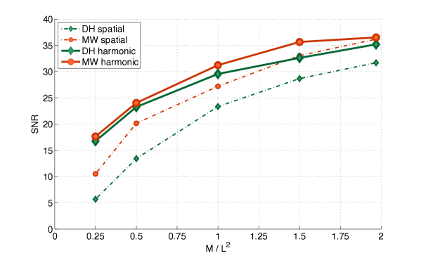
Figure 2: Reconstruction performance for the DH and MW sampling theorems

4 CONCLUSIONS

Although compressive sensing states that sparse or compressible signals may be acquired with fewer samples than standard sampling theorems would suggest, the sampling theorem adopted nevertheless has an important influence on the performance of compressive sensing reconstruction. In Euclidean space, Shannon’s sampling theorem provides an optimal sampling for regular grids, leading to a unique sampling theorem. On the sphere, however, no sampling theorem is optimal, with different sampling theorems requiring a differing number of samples. The MW sampling theorem[3] has been developed only recently and achieves a more efficient sampling of the sphere than alternatives, requiring fewer than half as many samples as the canonical DH sampling theorem[4], while still capturing all of the information content of a band-limited signal. A reduction by a factor of two in the number of samples between the DH and MW sampling theorems has important implications for compressive sensing on the sphere, both in terms of the dimensionality and sparsity of signals. The more efficient sampling of the MW sampling theorem has been shown to enhance the performance of compressed sensing reconstruction on the sphere, as illustrated with an inpainting problem.[7]

- [1] Cooley, J. W. and Tukey, J. W., “An algorithm for the machine calculation of complex fourier series,” Math. Comp. 19, 297–301 (1965).
- [2] Shannon, C. E., “Communication in the presence of noise,” Proc. IRE 37, 10–21 (1949).
- [3] McEwen, J. D. and Wiaux, Y., “A novel sampling theorem on the sphere,” IEEE Trans. Sig. Proc. in press (2011).
- [4] Driscoll, J. R. and Healy, D. M. J., “Computing Fourier transforms and convolutions on the sphere,” Advances in Applied Mathematics 15, 202–250 (1994).
- [5] Candès, E., Romberg, J., and Tao, T., “Robust uncertainty principles: exact signal reconstruction from highly incomplete frequency information,” IEEE Trans. Inform. Theory 52, 489–509 (feb 2006).
- [6] Donoho, D., “Compressed sensing,” IEEE Trans. Inform. Theory 52, 1289–1306 (apr 2006).
- [7] McEwen, J. D., Puy, G., Thiran, J.-P., Vandergheynst, P., Ville, D. V. D., and Wiaux, Y., “Efficient and compressive sampling on the sphere,” IEEE Trans. Sig. Proc. submitted (2011).
- [8] Healy, D. M. J., Rockmore, D., Kostelec, P. J., and Moore, S. S. B., “FFTs for the 2-sphere – improvements and variations,” J. Fourier Anal. and Appl. 9(4), 341–385 (2003).
- [9] Risbo, T., “Fourier transform summation of Legendre series and -functions,” J. Geodesy 70(7), 383–396 (1996).
- [10] Goldberg, J. N., Macfarlane, A. J., Newman, E. T., Rohrlich, F., and Sudarshan, E. C. G., “Spin- spherical harmonics and ,” J. Math. Phys. 8(11), 2155–2161 (1967).
- [11] Varshalovich, D. A., Moskalev, A. N., and Khersonskii, V. K., [Quantum theory of angular momentum ], World Scientific, Singapore (1989).
- [12] Nikiforov, A. F. and Uvarov, V. B., [Classical Orthogonal Polynomials of a Discrete Variable ], Springer-Verlag, Berlin (1991).
- [13] Abrial, P., Moudden, Y., Starck, J.-L., Afeyan, B., Bobin, J., Fadili, J., and Nguyen, M. K., “Morphological component analysis and inpainting on the sphere: application in physics and astrophysics,” J. Fourier Anal. and Appl. 14(6), 729–748 (2007).
- [14] Rauhut, H. and Ward, R., “Sparse recovery for spherical harmonic expansions,” ArXiv:1102.4097 (2011).