The existence theorem for steady Navier–Stokes equations in the axially symmetric case

Abstract

We study the nonhomogeneous boundary value problem for Navier–Stokes equations of steady motion of a viscous incompressible fluid in a three–dimensional bounded domain with multiply connected boundary. We prove that this problem has a solution in some axially symmetric cases, in particular, when all components of the boundary intersect the axis of symmetry.

1 Introduction

Let $\Omega$ be a bounded domain in ${\mathbb{R}}^{3}$ with with multiply connected Lipschitz boundary $\partial\Omega$ consisting of $N+1$ disjoint components $\Gamma_{j}$: $\partial\Omega=\Gamma_{0}\cup\ldots\cup\Gamma_{N}$, and $\Gamma_{i}\cap\Gamma_{j}=\emptyset,\,i\neq j$. Consider in $\Omega$ the stationary Navier–Stokes system with nonhomogeneous boundary conditions

$$\left\{\begin{array}[]{rcl}-\nu\Delta{\bf u}+\big{(}{\bf u}\cdot\nabla\big{)}{\bf u}+\nabla p&=&{0}\qquad\hbox{\rm in }\;\;\Omega,\\[4.0pt] \mathop{\rm div}\,{\bf u}&=&0\qquad\hbox{\rm in }\;\;\Omega,\\[4.0pt] {\bf u}&=&{\bf a}\qquad\hbox{\rm on }\;\;\partial\Omega.\end{array}\right.$$ (1.1)

The continuity equation $(\ref{NS}_{2})$ implies the necessary compatibility condition for the solvability of problem (1.1):

$$\intop\limits_{\partial\Omega}{\bf a}\cdot{\bf n}\,dS=\sum\limits_{j=0}^{N}\intop\limits_{\Gamma_{j}}{\bf a}\cdot{\bf n}\,dS=\sum\limits_{j=0}^{N}{\mathcal{F}}_{i}=0,$$ (1.2)

where ${\bf n}$ is a unit vector of the outward (with respect to $\Omega$) normal to $\partial\Omega$ and ${\mathcal{F}}_{j}=\intop\limits_{\Gamma_{j}}{\bf a}\cdot{\bf n}\,dS$.

Starting from the famous paper of J. Leray [22] published in 1933, problem (1.1) was a subject of investigation in many papers (see, e.g., [1], [2], [7]–[12], [17]–[20], [25]–[34], etc.). However, for a long time the existence of a weak solution ${\bf u}\in W^{1,2}(\Omega)$ to problem (1.1) was proved only under the condition

$${{\mathcal{F}}}_{j}=\intop\limits_{\Gamma_{j}}{\bf a}\cdot{\bf n}\,dS=0,\qquad j=1,2,\ldots,N,$$ (1.3)

or for sufficiently small fluxes (see [22], [19]–[20], [8], [34], [17], etc.). Condition (1.3) requires the net flux ${{\mathcal{F}}}_{j}$ of the boundary value ${\bf a}$ to be zero separately across each component $\Gamma_{j}$ of the boundary $\partial\Omega$, while the compatibility condition (1.2) means only that the total flux is zero. Thus, (1.3) is stronger than (1.2) (condition (1.3) does not allow the presence of sinks and sources).

For a detailed survey of previous results one can see the recent papers [14] or [27]–[28]. In particular, in the last papers V.V. Pukhnachev has established the existence of a solution to problem (1.1) in the three–dimensional case when the domain $\Omega$ and the boundary value ${\bf a}$ have an axis of symmetry and a plane of symmetry which is perpendicular to this axis, moreover, this plane intersects each component of the boundary.

In this paper we study the problem in the axial symmetric case. Let $O_{x_{1}},O_{x_{2}},O_{x_{3}}$ be coordinate axis in ${\mathbb{R}}^{3}$ and $\theta=\mathop{\rm arctg}(x_{2}/x_{1})$, $r=(x_{1}^{2}+x_{2}^{2})^{1/2}$, $z=x_{3}$ be cylindrical coordinates. Denote by $v_{\theta},v_{r},v_{z}$ the projections of the vector $\bf v$ on the axes $\theta,r,z$.

A function $f$ is said to be axially symmetric if it does not depend on $\theta$. A vector-valued function ${\bf h}=(h_{\theta},h_{r},h_{z})$ is called axially symmetric if $h_{\theta}$, $h_{r}$ and $h_{z}$ do not depend on $\theta$. A vector-valued function ${\bf h}=(h_{\theta},h_{r},h_{z})$ is called axially symmetric without rotation if $h_{\theta}=0$ while $h_{r}$ and $h_{z}$ do not depend on $\theta$.

We will use the following symmetry assumptions.

(SO) $\Omega\subset{\mathbb{R}}^{3}$ is a bounded domain with Lipschitz boundary and $O_{x_{3}}$ is the axis of symmetry of the domain $\Omega$.

(AS) The assumptions (SO) are fulfilled and the boundary value ${\bf a}\in W^{1/2,2}(\partial\Omega)$ is axially symmetric.

(ASwR) The assumptions (SO) are fulfilled and the boundary value ${\bf a}\in W^{1/2,2}(\partial\Omega)$ is axially symmetric without rotation.

Denote by $\Omega_{j}$ the bounded simply connected domain with $\partial\Omega_{j}=\Gamma_{j}$, $j=0,\dots,N$. Let $\Omega_{0}$ be the largest domain, i.e.,

$$\Omega=\Omega_{0}\setminus\bigl{(}\cup_{j=1}^{N}\bar{\Omega}_{j}\bigr{)}.$$

Here and henceforth we denote by $\bar{A}$ the closure of the set $A$.

Let

$$\Gamma_{j}\cap O_{x_{3}}\neq\emptyset,\quad j=0,\dots,M,$$

$$\Gamma_{j}\cap O_{x_{3}}=\emptyset,\quad j=M+1,\dots,N.$$

We shall prove the existence theorem if one of the following two additional conditions is fulfilled:

$$M=N-1,\qquad{\mathcal{F}}_{N}\geq 0,$$ (1.4)

or

$$|{\mathcal{F}}_{j}|<\delta,\quad j=M+1,\ldots,N,$$ (1.5)

where $\delta=\delta(\nu,\Omega)$ is sufficiently small ($\delta(\nu,\Omega)$ is specified below in Section 4). In particular, (1.5) includes the case $N=M$, i.e, when each component of the boundary intersects the axis of symmetry. Notice that in (1.4), (1.5) the fluxes ${\mathcal{F}}_{j},j=1,\ldots,M$, could be arbitrary large.

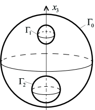
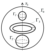
(a) M=N=2 (b) M=2, N=3 (c) M=1, N=3

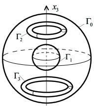
Figure 1: Domain $\Omega$

On Fig.1 we show several possible domains $\Omega$. In the case (a) all fluxes ${\mathcal{F}}_{0},{\mathcal{F}}_{1}$ and ${\mathcal{F}}_{2}$ are arbitrary; in the case (b) fluxes ${\mathcal{F}}_{0},{\mathcal{F}}_{1},{\mathcal{F}}_{2}$ are arbitrary, while the flux ${\mathcal{F}}_{3}$ has to be nonnegative, but there are no restriction on its size; in the case (c) fluxes ${\mathcal{F}}_{0},{\mathcal{F}}_{1}$ are arbitrary, while ${\mathcal{F}}_{2}$ and ${\mathcal{F}}_{3}$ has to be ”sufficiently small”.

The main result of the paper reads as follows.

Theorem 1.1.

Let the conditions (AS), (1.2) be fulfilled. Suppose that one of the conditions (1.4) or (1.5) holds. Then the problem $(\ref{NS})$ admits at least one weak axially symmetric solution ${\bf u}\in W^{1,2}(\Omega)$.

If, in addition, the conditions (ASwR) are fulfilled, then the problem $(\ref{NS})$ admits at least one weak axially symmetric solution without rotation.

(For the definition of a weak solution, see Section 2.1.) The analogous results for the plane case were established in [14].

The proof of Theorem 1.1 uses the Bernoulli law for a weak solution of the Euler equations and the one-side maximum principle for the total head pressure corresponding to this solution (see Section 3). These results were obtained in [13] for plane case (see  [14] for more detailed proofs). The proof of the Bernoulli law for solutions from Sobolev spaces is based on recent results obtained in [3] (see also Section 2.2).

The short version of this paper was published in [15]. The preprint version of this paper see in [16].

2 Notations and preliminary results

By a domain we mean an open connected set. Let $\Omega\subset{\mathbb{R}}^{3}$ be a bounded domain with Lipschitz boundary $\partial\Omega$. We use standard notations for function spaces: $C^{k}(\bar{\Omega})$, $C^{k}(\partial\Omega)$, $W^{k,q}(\Omega)$, $\mathop{\mathaccent 23{W}^{k,q}}\nolimits(\Omega)$, $W^{\alpha,q}(\partial\Omega)$, where $\alpha\in(0,1),k\in{\mathbb{N}}_{0},q\in[1,+\infty]$. In our notation we do not distinguish function spaces for scalar and vector valued functions; it is clear from the context whether we use scalar or vector (or tensor) valued function spaces. $H(\Omega)$ is subspace of all solenoidal vector fields ($\mathop{\rm div}{\bf u}=0$) from $\mathop{\mathaccent 23{W}^{1,2}}\nolimits(\Omega)$ with the norm $\|{\bf u}\|_{H(\Omega)}=\|\nabla{\bf u}\|_{L^{2}(\Omega)}$. Note that for functions ${\bf u}\in H(\Omega)$ the norm $\|\cdot\|_{H(\Omega)}$ is equivalent to $\|\cdot\|_{W^{1,2}(\Omega)}$.

Working with Sobolev functions we always assume that the ”best representatives” are chosen. If $w\in L^{1}_{{\rm loc}}(\Omega)$, then the best representative $w^{*}$ is defined by

$$w^{*}(x)=\left\{\begin{array}[]{rcl}\lim\limits_{r\to 0}\mathchoice{{\vbox{\hbox{$\textstyle-$}}\kern-4.86108pt}}{{\vbox{\hbox{$\scriptstyle-$}}\kern-3.25pt}}{{\vbox{\hbox{$\scriptscriptstyle-$}}\kern-2.29166pt}}{{\vbox{\hbox{$\scriptscriptstyle-$}}\kern-1.875pt}}\!\intop_{B_{r}(x)}{w}(z)dz,&{\rm\;if\;the\;finite\;limit\;exists;}\\[4.0pt] 0&\;{\rm otherwise},\end{array}\right.$$

where $\mathchoice{{\vbox{\hbox{$\textstyle-$}}\kern-4.86108pt}}{{\vbox{\hbox{$\scriptstyle-$}}\kern-3.25pt}}{{\vbox{\hbox{$\scriptscriptstyle-$}}\kern-2.29166pt}}{{\vbox{\hbox{$\scriptscriptstyle-$}}\kern-1.875pt}}\!\intop_{B_{r}(x)}{w}(z)dz=\frac{1}{\mathop{\rm meas}(B_{r}(x))}\intop_{B_{r}(x)}{w}(z)dz$, $B_{r}(x)=\{y:|y-x|<r\}$ is a ball of radius $r$ centered at $x$.

Further (see Theorem 3.4) we will discuss some properties of the best representatives of Sobolev functions.

2.1 Some facts about solenoidal functions

The next lemmas concern the existence of a solenoidal extensions of boundary values and the integral representation of the bounded linear functionals vanishing on solenoidal functions.

Lemma 2.1 (see Corollary 2.3 in [21]).

Let $\Omega\subset{\mathbb{R}}^{3}$ be a bounded domain with Lipschitz boundary. If ${\bf a}\in W^{1/2,2}(\partial\Omega)$ and the equality (1.2) is fulfilled, then there exists a solenoidal extension ${\bf A}\in W^{1,2}(\Omega)$ of ${\bf a}$ such that

$$\|{\bf A}\|_{W^{1,2}(\Omega)}\leq c\|{\bf a}\|_{W^{1/2,2}(\partial\Omega)}.$$ (2.1)

From this Lemma we can deduce some assertions for the symmetric case.

Lemma 2.2.

Let the conditions (AS), (1.2) be fulfilled. Then there exists an axially symmetric solenoidal extension ${\bf A}\in W^{1,2}(\Omega)$ of ${\bf a}$ such that the estimate (2.1) holds.

Proof. Let ${\bf A_{0}}\in W^{1,2}(\Omega)$ be solenoidal extension of ${\bf a}$ from Lemma 2.1. Put

$${\bf A}_{i}(\theta,r,z)=\frac{1}{i!}\sum\limits_{j=0}^{i!}{\bf A_{0}}\bigl{(}\theta+\frac{2\pi j}{i!},r,z\bigr{)}.$$

Clearly, each ${\bf A}_{i}$ is also solenoidal extension of ${\bf a}$ and the estimate (2.1) holds for ${\bf A}_{i}$ with the same $c$ (not depending on $i$). By construction

$${\bf A}_{i}(\theta+\frac{2\pi j}{m},r,z)={\bf A}_{i}(\theta,r,z)\quad\mbox{for all }m=1,\dots,i.$$ (2.2)

Take a weakly convergence sequence ${\bf A}_{i_{k}}\rightharpoonup{\bf A}$ in $W^{1,2}(\Omega)$. Then by construction $\mathop{\rm div}{\bf A}=0$,  ${\bf A}|_{\partial\Omega}={\bf a}$, and the estimate (2.1) holds. From (2.2) it follows that ${\bf A}(\theta+\frac{2\pi j}{m},r,z)={\bf A}(\theta,r,z)$ for all $m,j$. Hence $\bf A$ is axially symmetric. ∎

Lemma 2.3.

Let the conditions (ASwR), (1.2) be fulfilled. Then there exists a solenoidal extension ${\bf A}\in W^{1,2}(\Omega)$ of ${\bf a}$ such that ${\bf A}$ is axially symmetric without rotation and the estimate (2.1) holds.

Proof. Let ${\bf\tilde{A}}=(\tilde{A}_{\theta},\tilde{A}_{r},\tilde{A}_{z})\in W^{1,2}(\Omega)$ be solenoidal extension of ${\bf a}$ from the previous Lemma 2.2. Then by classical formula

$$\begin{array}[]{rcl}\operatorname{div}\mathbf{\tilde{A}}(\theta,r,z)=\frac{1}{r}\frac{\partial}{\partial\theta}(\tilde{A}_{\theta})+\frac{1}{r}\frac{\partial}{\partial r}(\tilde{A}_{r}r)+\frac{\partial}{\partial z}(\tilde{A}_{z})\\[4.0pt] =\frac{1}{r}\frac{\partial}{\partial r}(\tilde{A}_{r}r)+\frac{\partial}{\partial z}(\tilde{A}_{z})=0.\end{array}$$ (2.3)

Here $\frac{\partial\tilde{A}_{\theta}}{\partial\theta}=0$ because of axial symmetry. Define the vector field ${\bf A}=(A_{\theta},A_{r},A_{z})$ by the formulas

$$A_{\theta}=0,\quad A_{r}=\tilde{A}_{r},\quad A_{z}=\tilde{A}_{z}.$$

Then by construction ${\bf A}$ is axially symmetric without rotation, ${\bf A}|_{\partial\Omega}={\bf a}$, and the estimate (2.1) holds. From (2.3) it follows that $\mathop{\rm div}{\bf A}=0$. ∎

Lemma 2.4 (see [31]).

Let $\Omega\subset{\mathbb{R}}^{3}$ be a bounded domain with Lipschitz boundary and $R(\boldsymbol{\eta})$ be a continuous linear functional defined on $\mathop{\mathaccent 23{W}^{1,2}}\nolimits(\Omega)$. If

$$R(\boldsymbol{\eta})=0\qquad\forall\;\;\boldsymbol{\eta}\in H(\Omega),$$

then there exists a unique function $p\in L^{2}(\Omega)$ with $\intop\limits_{\Omega}p(x)\,dx=0$ such that

$$R(\boldsymbol{\eta})=\intop\limits_{\Omega}p\,{\rm div}\,\boldsymbol{\eta}\,dx\qquad\forall\;\;\boldsymbol{\eta}\in\mathop{\mathaccent 23{W}^{1,2}}\nolimits(\Omega).$$

Moreover, $\|p\|_{L^{2}(\Omega)}$ is equivalent to $\|R\|_{(\mathop{\mathaccent 23{W}^{1,2}}\nolimits(\Omega))^{*}}$.

Lemma 2.5.

If, in addition to conditions of Lemma 2.4, the domain $\Omega$ satisfies the assumption (SO) and $R(\boldsymbol{\eta})\equiv R(\boldsymbol{\eta}_{\theta_{0}})$ for all $\boldsymbol{\eta}\in H(\Omega)$, $\theta_{0}\in[0,2\pi]$, where $\boldsymbol{\eta}_{\theta_{0}}(\theta,r,z):=\boldsymbol{\eta}(\theta+\theta_{0},r,z)$, then the function $p$ is axially symmetric.

Proof. Take the function $p$ from the assertion of Lemma 2.4. For $\theta_{0}\in[0,2\pi]$ define the function $p_{\theta_{0}}$ by the formula $p_{\theta_{0}}(\theta,r,z):=p(\theta-\theta_{0},r,z)$. By construction,

$$\intop\limits_{\Omega}p\,{\rm div}\,\boldsymbol{\eta}\,dx=R(\boldsymbol{\eta})=R(\boldsymbol{\eta}_{\theta_{0}})=\intop\limits_{\Omega}p\,{\rm div}\,\boldsymbol{\eta}_{\theta_{0}}\,dx$$

$$=\intop\limits_{\Omega}p_{\theta_{0}}{\rm div}\,\boldsymbol{\eta}\,dx\qquad\forall\;\;\boldsymbol{\eta}\in\mathop{\mathaccent 23{W}^{1,2}}\nolimits(\Omega).$$

Since $p$ is unique, we obtain the identity $p(x)\equiv p_{\theta_{0}}(x)$. ∎

Lemma 2.6 (see [20]).

Let $\Omega\subset{\mathbb{R}}^{3}$ be a bounded domain with Lipschitz boundary and let ${\bf A}\in W^{1,2}(\Omega)$ be divergence free. Then there exists a unique weak solution ${\bf U}\in W^{1,2}(\Omega)$ of the Stokes problem satisfying the boundary condition ${\bf U}|_{\partial\Omega}={\bf A}|_{\partial\Omega}$, i.e., ${\bf U}-{\bf A}\in H(\Omega)$ and

$$\intop\limits_{\Omega}\nabla{\bf U}\cdot\nabla\boldsymbol{\eta}\,dx=0\quad\forall\;\boldsymbol{\eta}\in H(\Omega).$$ (2.4)

Moreover,

$$\|{\bf U}\|_{W^{1,2}(\Omega)}\leq c\|{\bf A}\|_{W^{1,2}(\Omega)}.$$ (2.5)

Lemma 2.7.

If, in addition to conditions of Lemma 2.6, the domain $\Omega$ satisfies the assumptions (SO) and also $\bf A$ is axially symmetric, then $\bf U$ is axially symmetric too.

Proof. Let $\bf U$ be a solution of the Stokes problem from Lemma 2.6. For $\theta_{0}\in[0,2\pi]$ define the function ${\bf U}_{\theta_{0}}$ by the formula ${\bf U}_{\theta_{0}}(\theta,r,z):={\bf U}(\theta-\theta_{0},r,z)$. By construction, ${\bf U}_{\theta_{0}}-{\bf A}\in H(\Omega)$. Moreover,

$$\intop\limits_{\Omega}\nabla{\bf U}_{\theta_{0}}\cdot\nabla\boldsymbol{\eta}\,dx=\intop\limits_{\Omega}\nabla{\bf U}\cdot\nabla\boldsymbol{\eta}_{\theta_{0}}\,dx=0\quad\ \forall\;\boldsymbol{\eta}\in H(\Omega),$$

where $\boldsymbol{\eta}_{\theta_{0}}(\theta,r,z):=\boldsymbol{\eta}(\theta+\theta_{0},r,z)$. Because of the uniqueness, we obtain the identity ${\bf U}(x)\equiv{\bf U}_{\theta_{0}}(x)$. ∎

Lemma 2.8.

If, in addition to conditions of Lemma 2.6, the vector field $\bf A$ is axially symmetric without rotation, then $\bf U$ is axially symmetric without rotation too.

Proof. Take the function ${\bf U}=(U_{\theta},U_{r},U_{z})$ from the assertion of Lemma 2.6 and define $\boldsymbol{\eta}=(\eta_{\theta},\eta_{r},\eta_{z})$ by the formulas

$$\eta_{\theta}\equiv U_{\theta},\quad\eta_{r}=\eta_{z}\equiv 0.$$

Then from Lemma 2.7 it follows the inclusion $\boldsymbol{\eta}\in H(\Omega)$ (see also the formula (2.3)). Consequently, from (2.4) we obtain

$$\intop\limits_{\Omega}\nabla{\bf U}\cdot\nabla\boldsymbol{\eta}\,dx=0.$$ (2.6)

But by the direct calculation

$$\nabla{\bf U}\cdot\nabla\boldsymbol{\eta}\equiv\biggl{(}\frac{U_{\theta}}{r}\biggr{)}^{2}+\biggl{(}\frac{\partial U_{\theta}}{\partial r}\biggr{)}^{2}+\biggl{(}\frac{\partial U_{\theta}}{\partial z}\biggr{)}^{2}.$$ (2.7)

Formulas (2.6), (2.7) imply the required equality $U_{\theta}\equiv 0$. ∎

For a function ${\bf f}\in L^{q}(\Omega),1\leq q\leq 6/5$, consider a continuous linear functional $H(\Omega)\ni\boldsymbol{\eta}\mapsto\intop\limits_{\Omega}{\bf f}\cdot\boldsymbol{\eta}\,dx$. Because of Riesz representation theorem there exists a unique function ${\bf g}\in H(\Omega)$ such that

$$\intop\limits_{\Omega}{\bf f}\cdot\boldsymbol{\eta}\,dx=\intop\limits_{\Omega}\nabla\boldsymbol{\eta}\cdot\nabla{\bf g}\,dx=\langle{\bf g},\boldsymbol{\eta}\rangle_{H(\Omega)}\quad\forall\boldsymbol{\eta}\in H(\Omega).$$

Denote ${\bf g}=T_{0}{\bf f}$. Evidently, $T_{0}$ is a continuous linear operator from $L^{q}(\Omega)$ to $H(\Omega)$.

Denote by $L^{q}_{AS}(\Omega)$ the space of all axially symmetric vector-function from $L^{q}(\Omega)$. Analogously define the spaces $L^{q}_{ASwR}(\Omega)$, $H_{AS}(\Omega)$, $H_{ASwR}(\Omega)$, $W^{1,2}_{AS}(\Omega)$, $W^{1,2}_{ASwR}(\Omega)$, etc.

Lemma 2.9.

The operator $T_{0}:L^{3/2}(\Omega)\to H(\Omega)$ has the following symmetry properties:

$$\forall{\bf f}\in L^{3/2}_{AS}(\Omega)\quad T_{0}{\bf f}\in H_{AS}(\Omega),$$ (2.8)

$$\forall{\bf f}\in L^{3/2}_{ASwR}(\Omega)\quad T_{0}{\bf f}\in H_{ASwR}(\Omega).$$ (2.9)

Proof. The property (2.8) can be proved in the same way as Lemma 2.7 and the property (2.9) as Lemma 2.8. ∎

Lemma 2.10.

The following inclusions are fulfilled:

$$\forall{\bf u},{\bf v}\in H_{AS}(\Omega)\qquad({\bf u}\cdot\nabla){\bf v}\in L^{3/2}_{AS}(\Omega),$$ (2.10)

$$\forall{\bf u},{\bf v}\in H_{ASwR}(\Omega)\qquad({\bf u}\cdot\nabla){\bf v}\in L^{3/2}_{ASwR}(\Omega).$$ (2.11)

Proof. by direct calculation. ∎

Assume that ${\bf a}\in W^{1/2,2}(\partial\Omega)$ and let conditions $(\ref{flux})$, (AS) (or (ASwR) ) be fulfilled. Take the corresponding axially symmetric functions $\bf A$, $\bf U$ from the above Lemmas. Denote ${\bf w}={\bf u}-{\mathbf{U}}$. Then the problem (1.1) is equivalent to the following one

$$\left\{\begin{array}[]{rcl}-\nu\Delta{\bf w}+\big{(}{\bf U}\cdot\nabla\big{)}{\bf w}+\big{(}{\bf w}\cdot\nabla\big{)}{\bf w}+\big{(}{\bf w}\cdot\nabla\big{)}{\bf U}\\[4.0pt] =-\nabla p-\big{(}{\bf U}\cdot\nabla\big{)}{\bf U}\qquad\hbox{\rm in }\;\;\Omega,\\[4.0pt] \mathop{\rm div}\,{\bf w}=0\qquad\hbox{\rm in }\;\;\Omega,\\[4.0pt] {\bf w}=0\qquad\hbox{\rm on }\;\;\partial\Omega.\end{array}\right.$$ (2.12)

By a weak solution of problem (1.1) we understand a function ${\bf u}$ such that ${\bf w}={\bf u}-{\bf U}\in H(\Omega)$ and

$$\nu\langle{\bf w},\boldsymbol{\eta}\rangle_{H(\Omega)}=-\intop\limits_{\Omega}\big{(}{\bf U}\cdot\nabla\big{)}{\bf U}\cdot\boldsymbol{\eta}\,dx-\intop\limits_{\Omega}\big{(}{\bf U}\cdot\nabla\big{)}{\bf w}\cdot\boldsymbol{\eta}\,dx$$

$$-\intop\limits_{\Omega}\big{(}{\bf w}\cdot\nabla\big{)}{\bf w}\cdot\boldsymbol{\eta}\,dx-\intop\limits_{\Omega}\big{(}{\bf w}\cdot\nabla\big{)}{\bf U}\cdot\boldsymbol{\eta}\,dx\qquad\forall\boldsymbol{\eta}\in H(\Omega).$$ (2.13)

Because of Riesz representation theorem for any ${\bf w}\in H(\Omega)$ there exists a unique function $T{\bf w}\in H(\Omega)$ such that the right-hand side of the equality (2.13) is equivalent to $\langle T{\bf w},\boldsymbol{\eta}\rangle_{H(\Omega)}$ for all $\boldsymbol{\eta}\in H(\Omega)$. Obviously, $T$ is a nonlinear operator from $H(\Omega)$ to $H(\Omega)$.

Lemma 2.11.

The operator $T:H(\Omega)\to H(\Omega)$ is a compact operator. Moreover, $T$ has the following symmetry properties:

$$\forall{\bf w}\in H_{AS}(\Omega)\quad T{\bf w}\in H_{AS}(\Omega),$$ (2.14)

$$\forall{\bf w}\in H_{ASwR}(\Omega)\quad T{\bf w}\in H_{ASwR}(\Omega).$$ (2.15)

Proof. The first statement is well known (see [20]). The statements about symmetry follow from the above Lemmas. ∎

Obviously, the identity (2.13) is equivalent to the operator equation in the space $H(\Omega)$:

$$\nu{\bf w}=T{\bf w}.$$ (2.16)

Thus, we can apply the Leray–Schauder fixed point Theorem to the compact operators $T|_{H_{AS}(\Omega)}$ and $T|_{H_{ASwR}(\Omega)}$. There hold the following statements.

Lemma 2.12.

Let the conditions (AS), $(\ref{flux})$ be fulfilled. Suppose that all possible solutions of the equation $\nu{\bf w}=\lambda T{\bf w}$, $\lambda\in[0,1]$, ${\bf w}\in H_{AS}(\Omega),$ are uniformly bounded in $H_{AS}(\Omega)$. Then the problem $(\ref{NS})$ admits at least one weak axially symmetric solution.

Lemma 2.13.

Let the conditions (ASwR), $(\ref{flux})$ be fulfilled. Suppose that all possible solutions of the equation $\nu{\bf w}=\lambda T{\bf w}$, $\lambda\in[0,1]$, ${\bf w}\in H_{ASwR}(\Omega),$ are uniformly bounded in $H_{ASwR}(\Omega)$. Then the problem $(\ref{NS})$ admits at least one weak axially symmetric solution without rotation.

2.2 On Morse-Sard and Luzin N-properties of Sobolev functions from $W^{2,1}$

First we recall some classical differentiability properties of Sobolev functions.

Lemma 2.14 (see Proposition 1 in [5]).

Let $\psi\in W^{2,1}({\mathbb{R}}^{2})$. Then the function $\psi$ is continuous and there exists a set $A_{\psi}$ such that $\mathfrak{H}^{1}(A_{\psi})=0$, and the function $\psi$ is differentiable (in the classical sense) at each $x\in{\mathbb{R}}^{2}\setminus A_{\psi}$. Furthermore, the classical derivative at such points $x$ coincides with $\nabla\psi(x)=\lim\limits_{r\to 0}\mathchoice{{\vbox{\hbox{$\textstyle-$}}\kern-4.86108pt}}{{\vbox{\hbox{$\scriptstyle-$}}\kern-3.25pt}}{{\vbox{\hbox{$\scriptscriptstyle-$}}\kern-2.29166pt}}{{\vbox{\hbox{$\scriptscriptstyle-$}}\kern-1.875pt}}\!\intop_{B_{r}(x)}{\nabla\psi}(z)dz$, where  $\lim\limits_{r\to 0}\mathchoice{{\vbox{\hbox{$\textstyle-$}}\kern-4.86108pt}}{{\vbox{\hbox{$\scriptstyle-$}}\kern-3.25pt}}{{\vbox{\hbox{$\scriptscriptstyle-$}}\kern-2.29166pt}}{{\vbox{\hbox{$\scriptscriptstyle-$}}\kern-1.875pt}}\!\intop\nolimits_{B_{r}(x)}|\nabla\psi(z)-\nabla\psi(x)|^{2}dz=0$.

Here and henceforth we denote by $\mathfrak{H}^{1}$ the one-dimensional Hausdorff measure, i.e., $\mathfrak{H}^{1}(F)=\lim\limits_{t\to 0+}\mathfrak{H}^{1}_{t}(F)$, where $\mathfrak{H}^{1}_{t}(F)=\inf\{\sum\limits_{i=1}^{\infty}{\rm diam}F_{i}:\,{\rm diam}F_{i}\leq t,F\subset\bigcup\limits_{i=1}^{\infty}F_{i}\}$.

The next theorems have been proved recently by J. Bourgain, M. Korobkov and J. Kristensen [3].

Theorem 2.1.

Let ${\mathcal{D}}\subset{\mathbb{R}}^{2}$ be a bounded domain with Lipschitz boundary and $\psi\in W^{2,1}({\mathcal{D}})$. Then

(i) $\mathfrak{H}^{1}(\{\psi(x)\,:\,x\in\bar{\mathcal{D}}\setminus A_{\psi}\,\,\&\,\,\nabla\psi(x)=0\})=0$;

(ii) for every $\varepsilon>0$ there exists $\delta>0$ such that for any set $U\subset\bar{\mathcal{D}}$ with $\mathfrak{H}^{1}_{\infty}(U)<\delta$ the inequality $\mathfrak{H}^{1}(\psi(U))<\varepsilon$ holds.

(iii) for $\mathfrak{H}^{1}$–almost all $y\in\psi(\bar{\mathcal{D}})\subset\mathbb{R}$ the preimage $\psi^{-1}(y)$ is a finite disjoint family of $C^{1}$–curves $S_{j}$, $j=1,2,\ldots,N(y)$. Each $S_{j}$ is either a cycle in ${\mathcal{D}}$ $($i.e., $S_{j}\subset{\mathcal{D}}$ is homeomorphic to the unit circle $\mathbb{S}^{1})$ or it is a simple arc with endpoints on $\partial{\mathcal{D}}$ $($in this case $S_{j}$ is transversal to $\partial{\mathcal{D}}\,)$.

Theorem 2.2.

Let $\mathcal{D}\subset{\mathbb{R}}^{2}$ be a bounded domain with Lipschitz boundary and $\psi\in W^{2,1}(\mathcal{D})$. Then for every $\varepsilon>0$ there exists an open set $V\subset\mathbb{R}$ and a function $g\in C^{1}(\mathbb{R}^{2})$ such that $\mathfrak{H}^{1}(V)<\varepsilon$, and for each $x\in\bar{\mathcal{D}}$ if $\psi(x)\notin V$ then $x\notin A_{\psi}$, the function $\psi$ is differentiable at the point $x$, and $\psi(x)=g(x)$, $\nabla\psi(x)=\nabla g(x)\neq 0$.

We shall say that a value $y\in\psi(\bar{\mathcal{D}})$ is regular if it satisfies the condition (iii) of Theorem 2.1 and $\psi(x)\notin V$ for some $g,V$ from Theorem 2.2. Note, that by above Theorems almost all values $y\in\psi(\bar{\mathcal{D}})$ are regular.

3 Euler equation

We will study the Euler equation under the following assumptions.

(E) Let the conditions (SO) be fulfilled. Suppose that some axially symmetric functions ${\bf v}\in W^{1,2}(\Omega)$ and $p\in W^{1,3/2}(\Omega)$ satisfy the Euler system

$$\left\{\begin{array}[]{rcl}\lambda_{0}\big{(}{\bf v}\cdot\nabla\big{)}{\bf v}+\nabla p&=&0,\\[4.0pt] \mathop{\rm div}{\mathbf{v}}&=&0\end{array}\right.$$ (3.1)

for almost all $x\in\Omega$. Moreover, suppose that

$${\bf v}|_{\partial\Omega}=0.$$ (3.2)

Denote $P_{+}=\{(0,{x_{2}},{x_{3}}):{x_{2}}>0,\ {x_{3}}\in{\mathbb{R}}\}$,  ${{\mathcal{D}}}=\Omega\cap P_{+}$, ${\mathcal{D}}_{j}=\Omega_{j}\cap P_{+}$. Of course, on $P_{+}$ the coordinates $x_{2},x_{3}$ coincides with coordinates $r,z$. From the conditions (SO) one can easily see that

(S₁) ${{\mathcal{D}}}$ is a bounded plane domain with Lipschitz boundary. Moreover, $C_{j}:=P_{+}\cap\Gamma_{j}$ is a connected set for each $j=0,\dots,N$. In other words, the family $\{C_{j}:j=0,\dots,N\}$ coincides with the family of all connected components of the set $P_{+}\cap\partial{{\mathcal{D}}}$.

Then ${\bf v}$ and $p$ satisfy the following system of equations in the plane domain ${\mathcal{D}}$:

$$\left\{\begin{array}[]{rcl}\frac{\partial p}{\partial z}+\lambda_{0}v_{r}\frac{\partial v_{z}}{\partial r}+\lambda_{0}v_{z}\frac{\partial v_{z}}{\partial z}=0,\\[6.0pt] \frac{\partial p}{\partial r}-\lambda_{0}\frac{(v_{\theta})^{2}}{r}+\lambda_{0}v_{r}\frac{\partial v_{r}}{\partial r}+\lambda_{0}v_{z}\frac{\partial v_{r}}{\partial z}=0,\\[6.0pt] \frac{v_{\theta}v_{r}}{r}+v_{r}\frac{\partial v_{\theta}}{\partial r}+v_{z}\frac{\partial v_{\theta}}{\partial z}=0,\\[6.0pt] \frac{\partial(rv_{r})}{\partial r}+\frac{\partial(rv_{z})}{\partial z}=0\end{array}\right.$$ (3.3)

(these equations are fulfilled for almost all $x\in{\mathcal{D}}$ ).

The next statement was proved in [12, Lemma 4] and in [1, Theorem 2.2].

Theorem 3.1.

Let the conditions (E) be fulfilled. Then

$$\forall j\in\{0,\dots,N\}\ \exists\,p_{j}\in{\mathbb{R}}:\quad p(x)\equiv p_{j}\quad\mbox{for }{\mathfrak{H}}^{2}-\mbox{almost all }x\in\Gamma_{j}.$$ (3.4)

In particular, by axial symmetry,

$$p(x)\equiv p_{j}\quad\mbox{for }{\mathfrak{H}}^{1}-\mbox{almost all }x\in C_{j}.$$ (3.5)

Lemma 3.1 (e.g., [17], [26]).

Under conditions of Theorem 3.1, the following estimate

$$\max\limits_{i,j=0,\dots N}|p_{i}-p_{j}|\leq\delta_{1}\lambda_{0}\|{\mathbf{v}}\|^{2}_{H(\Omega)}$$ (3.6)

holds, where the constant $\delta_{1}$ depends on $\Omega$ only.

One of the main purposes of this Section is to prove the following fact.

Theorem 3.2.

Under conditions of Theorem 3.1, the equalities

$$p_{0}=p_{1}=\dots=p_{M}$$ (3.7)

are fulfilled.

To prove the last Theorem, we need some preparation, especially, a version of Bernoulli Law for Sobolev case (see below Theorem 3.3).

From the last equality in (3.3) and from (3.2) it follows that there exists a stream function $\psi\in W^{2,2}_{{\rm loc}}({\mathcal{D}})$ such that

$$\frac{\partial\psi}{\partial r}=-rv_{z},\quad\frac{\partial\psi}{\partial z}=rv_{r}.$$ (3.8)

We have the following integral estimates: ${\bf v}\in W^{1,2}_{\rm loc}({\mathcal{D}})$,

$$\intop_{{\mathcal{D}}}r|{\bf v}(r,z)|^{2}\,drdz<\infty.$$ (3.9)

By identities (3.8), we can rewrite the last formula in the following way:

$$\intop_{{\mathcal{D}}}\frac{|\nabla\psi(r,z)|^{2}}{r}\,drdz<\infty.$$ (3.10)

Fix a point $x_{*}\in{\mathcal{D}}$. For $\varepsilon>0$ denote by ${\mathcal{D}}_{\varepsilon}$ the connected component of ${\mathcal{D}}\cap\{(r,z):r>\varepsilon\}$ containing $x_{*}$. Since

$$\psi\in W^{2,2}({\mathcal{D}}_{\varepsilon})\quad\forall\varepsilon>0,$$ (3.11)

by Sobolev Embedding Theorem $\psi\in C(\bar{\mathcal{D}}_{\varepsilon})$. Hence $\psi$ is continuous at points from $\bar{\mathcal{D}}\setminus O_{z}=\bar{\mathcal{D}}\setminus\{(0,z):z\in{\mathbb{R}}\}$.

Denote by $\Phi=p+\lambda_{0}\dfrac{|{\bf v}|^{2}}{2}$ the total head pressure corresponding to the solution $({\bf v},p)$. Obviously,

$$\Phi\in W^{1,3/2}({\mathcal{D}}_{\varepsilon})\quad\forall\varepsilon>0.$$ (3.12)

By direct calculations one easily gets the identity

$$v_{r}\frac{\partial\Phi}{\partial r}+v_{z}\frac{\partial\Phi}{\partial z}=0$$ (3.13)

for almost all $x\in{\mathcal{D}}$.

Theorem 3.3.

Let the conditions (E) be valid (see the beginning of this Section). Then there exists a set $A_{\mathbf{v}}\subset P_{+}$ such that ${\mathfrak{H}}^{1}(A_{\mathbf{v}})=0$ and for any compact connected set $K\subset\bar{\mathcal{D}}\setminus O_{z}$, if

$$\psi\big{|}_{K}={\rm const},$$ (3.14)

then the identities

$$\Phi(x_{1})=\Phi(x_{2})\quad\mbox{for all \,}x_{1},x_{2}\in K\setminus A_{\bf v}$$ (3.15)

hold.

Theorem 3.3 was obtained for plane case in [13, Theorem 1] (see also [14] for detailed proof).

To prove Theorem 3.3, we need some preliminaries.

Lemma 3.2.

Let the conditions (E) be fulfilled. Then the inclusion

$$p\in W^{2,1}_{\rm loc}({\mathcal{D}})$$ (3.16)

holds.

Proof. Clearly, $p$ is the (unique) weak solution to the Poisson equation

$$\left\{\begin{array}[]{rcl}\Delta p+\lambda_{0}\nabla{\mathbf{v}}\cdot\nabla{\mathbf{v}}^{\top}&=&0\;\,\quad\hbox{\rm in }\Omega\\[4.0pt] p&=&\tilde{p},\quad\hbox{\rm in }\partial\Omega,\end{array}\right.$$ (3.17)

with $\tilde{p}=\hbox{\rm tr}\,_{|\partial\Omega}p\in W^{1/3,3/2}(\partial\Omega)$. Let

$$G(x)={\lambda_{0}\over 4\pi}\intop_{\Omega}{(\nabla{\mathbf{v}}\cdot\nabla{\mathbf{v}}^{\top})(y)\over|x-y|}dv_{y}.$$

By the results of [4] $\nabla{\mathbf{v}}\cdot\nabla{\mathbf{v}}^{\top}$ belongs to the Hardy space ${\cal H}^{1}$ so that by Calderón–Zygmund theorem for Hardy’s spaces [32] $G\in W^{2,1}(\Omega)$. Let $\bar{G}\in W^{1/3,3/2}(\partial\Omega)$ be the trace of $G$ on $\partial\Omega$ and let $p_{*}\in C^{\infty}(\Omega)$ be the solution to the problem

$$\left\{\begin{array}[]{rcl}\Delta p_{*}&=&0\qquad\quad\hbox{\rm in }\Omega,\\[4.0pt] p_{*}&=&\tilde{p}-\bar{G}\quad\hbox{\rm in }\partial\Omega.\end{array}\right.$$ (3.18)

By the uniqueness theorem

$$p=p_{*}+G(x)\in W^{2,1}_{\rm loc}(\Omega).$$

∎

From inclusion (3.16) it follows that  $p_{rz}\equiv p_{zr}$ for almost all $x\in{\mathcal{D}}$. Denote $Z=\{x\in{\mathcal{D}}:v_{r}(x)=v_{z}(x)=0\}$. Equations (3.3) yield the equality

$$\frac{\partial p}{\partial z}(x)=0,\quad\frac{\partial p}{\partial r}(x)=\lambda_{0}\frac{(v_{\theta})^{2}}{r}\quad\mbox{for almost all }x\in Z,$$

and it is easy to deduce that

$$\frac{\partial\Phi}{\partial z}(x)=0\quad\mbox{for almost all }x\in{\mathcal{D}}\mbox{ such that }v_{r}(x)=v_{z}(x)=0.$$ (3.19)

Consider the stream function $\psi$. From (3.2), (3.8) we have $\nabla\psi(x)=0$ for $\mathfrak{H}^{1}$-almost all $x\in\partial{\mathcal{D}}\setminus O_{z}$. Then from the Morse-Sard property (see Theorem 2.1) it follows that

$$\mbox{for \ any\ connected\ set\ }C\subset\partial{\mathcal{D}}\setminus O_{z}\ \exists\,\alpha=\alpha(C)\in{\mathbb{R}}:\quad\psi(x)\equiv\alpha\ \forall x\in C.$$

Then by (S₁) (see the beginning of Section 3)

$$\forall j\in\{0,\dots,N\}\ \ \exists\,\xi_{j}\in{\mathbb{R}}:\quad\psi(x)\equiv\xi_{j}\ \forall x\in C_{j}.$$ (3.20)

Remark 3.1.

Since $\nabla\psi=0$ on $\partial D\setminus O_{z}$ (in the sense of traces), we can extend the function $\psi$ to the whole half-plane $P_{+}$:

$$\psi(x):=\xi_{0},\ \,x\in P_{+}\setminus{\mathcal{D}}_{0},\quad\psi(x):=\xi_{j},\ \,x\in P_{+}\cap\bar{\mathcal{D}}_{j},\ j=1,\dots,N.$$ (3.21)

The functions ${\mathbf{v}},p,\Phi$ can be extended to $P_{+}$ as follows:

$${\mathbf{v}}(x):=0,\quad x\in P_{+}\setminus{\mathcal{D}},$$ (3.22)

$$p(x)=\Phi(x):=p_{0},\ \,x\in P_{+}\setminus{\mathcal{D}}_{0},\quad p(x)=\Phi(x):=p_{j},\ \,x\in P_{+}\cap\bar{\mathcal{D}}_{j},\ j=1,\dots,N.$$ (3.23)

Then the extended functions inherit the properties of the previous ones. Namely, formulas (3.3), (3.8)–(3.13), (3.19) are fulfilled with ${\mathcal{D}}$, ${\mathcal{D}}_{\varepsilon}$ replaced by $P_{+}$ and

$$P_{\varepsilon}:=\{(r,z):r\in[\varepsilon,\frac{1}{\varepsilon}],\ z\in[-\frac{1}{\varepsilon},\frac{1}{\varepsilon}]\}$$ (3.24)

respectively.

For $r_{0}>0$ denote by $L_{r_{0}}$ the straight line parallel to the $z$-axis:  $L_{r_{0}}=\{(r_{0},z):z\in{\mathbb{R}}\}$.

Working with Sobolev functions we always assume that the ”best representatives” are chosen. The basic properties of these ”best representatives” are collected in the following

Theorem 3.4.

There exists a set $A_{\bf v}\subset P_{+}$ such that:

(i) $\mathfrak{H}^{1}(A_{\bf v})=0$;

(ii) For all $x\in P_{+}\setminus A_{\bf v}$

$$\lim\limits_{r\to 0}\mathchoice{{\vbox{\hbox{$\textstyle-$}}\kern-4.86108pt}}{{\vbox{\hbox{$\scriptstyle-$}}\kern-3.25pt}}{{\vbox{\hbox{$\scriptscriptstyle-$}}\kern-2.29166pt}}{{\vbox{\hbox{$\scriptscriptstyle-$}}\kern-1.875pt}}\!\intop\nolimits_{B_{r}(x)}|{\bf v}(y)-{\bf v}(x)|^{2}dy=\lim\limits_{r\to 0}\mathchoice{{\vbox{\hbox{$\textstyle-$}}\kern-4.86108pt}}{{\vbox{\hbox{$\scriptstyle-$}}\kern-3.25pt}}{{\vbox{\hbox{$\scriptscriptstyle-$}}\kern-2.29166pt}}{{\vbox{\hbox{$\scriptscriptstyle-$}}\kern-1.875pt}}\!\intop\nolimits_{B_{r}(x)}|{\Phi}(y)-{\Phi}(x)|^{3/2}dy=0,$$

$$\lim\limits_{r\to 0}\frac{1}{r}\intop\nolimits_{B_{r}(x)}|\nabla\Phi(y)|^{3/2}dy=0,$$

moreover, the function $\psi$ is differentiable at $x$ and $\nabla\psi(x)=(-rv_{z}(x),rv_{r}(x))$;

(iii) For all $\varepsilon>0$ there exists an open set $U\subset\mathbb{R}^{2}$ such that $\mathfrak{H}^{1}_{\infty}(U)<\varepsilon$, $A_{\bf v}\subset U$, and the functions ${\bf v},\Phi$ are continuous in $P_{+}\setminus U$;

(iv) For each $x_{0}=(r_{0},z_{0})\in P_{+}\setminus A_{\bf v}$ and for any $\varepsilon>0$ the convergence

$$\lim\limits_{\rho\to 0+}\frac{1}{2\rho}{\mathfrak{H}}^{1}(E(x_{0},\varepsilon,\rho))\to 1$$ (3.25)

holds, where

$$E(x_{0},\varepsilon,\rho):=\{t\in(-\rho,\rho):\intop\limits_{r_{0}-\rho}^{r_{0}+\rho}\biggl{|}\frac{\partial\Phi}{\partial r}(r,z_{0}+t)\biggr{|}\,dr+\intop\limits_{z_{0}-\rho}^{z_{0}+\rho}\biggl{|}\frac{\partial\Phi}{\partial z}(r_{0}+t,z)\biggr{|}\,dz$$

$$+\sup\limits_{r\in[r_{0}-\rho,r_{0}+\rho]}|\Phi(r,z_{0}+t)-\Phi(x_{0})|+\sup\limits_{z\in[z_{0}-\rho,z_{0}+\rho]}|\Phi(r_{0}+t,z)-\Phi(x_{0})|<\varepsilon\}.$$

(v) Take any function $g\in C^{1}({\mathbb{R}}^{2})$ and a closed set $F\subset P_{+}$ such that $\nabla g\neq 0$ on $F$. Then for almost all $y\in g(F)$ and for all the connected components $K$ of the set $F\cap g^{-1}(y)$ the equality $K\cap A_{{\mathbf{v}}}=\emptyset$ holds, the restriction $\Phi|_{K}$ is an absolutely continuous function, and formulas (3.3), (3.13) are fulfilled ${\mathfrak{H}}^{1}$-almost everywhere on $K$.

Most of these properties are from [6]. For the detailed proof of Theorem 3.4 see, e.g., [14]. The last property (v) follows (by coordinate transformation, cf. [23, §1.1.7]) from the well-known fact that any function $f\in W^{1,1}$ is absolutely continuous along almost all coordinate lines. The same fact together with (3.19), (3.13) imply

Lemma 3.3.

For almost all $r_{0}>0$ the equality $L_{r_{0}}\cap A_{\mathbf{v}}=\emptyset$ holds, moreover, $p(r_{0},\cdot)$, ${\mathbf{v}}(r_{0},\cdot)$ are absolutely continuous functions (locally) and

$$\frac{\partial\Phi}{\partial z}(r_{0},z)=0\quad\mbox{for almost all }z\in{\mathbb{R}}\mbox{ such that }v_{r}(r_{0},z)=0.$$ (3.26)

Below we prove that for the set $A_{\mathbf{v}}$ from Theorem 3.4 the assertion of Bernoulli Law (Theorem 3.3) holds. Before we need some lemmas.

Lemma 3.4.

For almost all $y\in\psi(P_{+})$ the equality

$$\psi^{-1}(y)\cap A_{\mathbf{v}}=\emptyset$$ (3.27)

holds, and for each continuum $K\subset\psi^{-1}(y)$ the identities

$$\Phi(x_{1})=\Phi(x_{2})\quad\mbox{for all \,}x_{1},x_{2}\in K$$ (3.28)

are fulfilled.

Proof.

Fix any $\varepsilon>0$ and consider a function $g\in C^{1}({\mathbb{R}}^{2})$ and an open set $V$ with $\mathfrak{H}^{1}(V)<\varepsilon$ from Theorem 2.2 applied to the function $\psi|_{P_{\varepsilon}}$, where the rectangle $P_{\varepsilon}$ was defined by formula (3.24). Put $F=P_{\varepsilon}\setminus\psi^{-1}(V)$. Then $\psi(x)=g(x)$ and $\nabla\psi(x)=\nabla g(x)\neq 0$ for any $x\in F$. Thus, by Theorem 3.4 (v) for almost all $y\in\psi(P_{\varepsilon})\setminus V=g(F)$ and for any connected component $K$ of the set $\{x\in P_{\varepsilon}:\psi(x)=y\}$ the equality $K\cap A_{\mathbf{v}}=\emptyset$ holds and the restriction $\Phi|_{K}$ is absolutely continuous, moreover, for any $C^{1}$–smooth parametrization $\gamma:[0,1]\to K$ the identity (3.13) gives

$$[\Phi(\gamma(t))]^{\prime}=\nabla\Phi(\gamma(t))\cdot\gamma^{\prime}(t)=0\quad\mbox{for }{\mathfrak{H}}^{1}\mbox{-almost all }t\in[0,1]$$

(the last equality is valid because $\psi(x)={\rm const}$ on $K$ and, hence, $\nabla\psi(\gamma(t))\cdot\gamma^{\prime}(t)=r(-v_{z}(\gamma(t)),v_{r}(\gamma(t)))\cdot\gamma^{\prime}(t)=0$). So, we have $\Phi(x)={\rm const}$ on $K$. In view of arbitrariness of $\varepsilon>0$ we have proved the assertion of the Lemma. ∎

We need also some technical facts about continuity properties of $\Phi$ at ”good” points $x\in P_{+}\setminus A_{\mathbf{v}}$.

Lemma 3.5.

Let $x_{0}\in P_{+}\setminus A_{\mathbf{v}}$. Suppose that there exist a constant $\sigma>0$ and a sequence of continuums $K_{j}\subset P_{+}\setminus A_{\mathbf{v}}$ such that $\Phi|_{K_{j}}\equiv\beta_{j}$, $K_{j}\subset B_{x_{0}}(\rho_{j})$, $\rho_{j}\to 0$ as $j\to\infty$, and $\mathop{\rm diam}(K_{j})\geq\sigma\rho_{j}$. Then $\beta_{j}\to\Phi(x_{0})$ as $j\to\infty$.

Proof. Without loss of generality we may assume that the projection of each $K_{j}$ on the $O_{r}$-axis is a segment $I_{j}\subset[r_{0}-\rho_{j},r_{0}+\rho_{j}]$ of the length $\frac{1}{2}\sigma\rho_{j}$ (otherwise the corresponding fact is valid for projection of $K_{j}$ on the $O_{z}$-axis, etc.) So by Theorem 3.4 (iv) for any $\varepsilon>0$ we have $I_{j}-\{r_{0}\}\cap E(x_{0},\varepsilon,\rho_{j})\neq\emptyset$ for sufficiently large $j$. Thus $|\beta_{j}-\Phi(x_{0})|<\varepsilon$ for sufficiently large $j$. ∎

Lemma 3.6.

Suppose for $r_{0}>0$ the assertion of Lemma 3.3 is fulfilled, i.e., the equality $L_{r_{0}}\cap A_{\mathbf{v}}=\emptyset$ holds, $p(r_{0},\cdot)$, ${\mathbf{v}}(r_{0},\cdot)$ are absolutely continuous functions, and formula (3.26) is valid. Let $F\subset{\mathbb{R}}$ be a compact set such that

$$\psi(r_{0},z)\equiv{\rm const}\quad\mbox{for all }z\in F$$ (3.29)

and

$$\Phi(r_{0},\alpha)=\Phi(r_{0},\beta)\quad\mbox{ for any interval }(\alpha,\beta)\mbox{ adjoining }F$$ (3.30)

(recall that $(\alpha,\beta)$ is called an interval adjoining $F$ if $\alpha,\beta\in F$ and $(\alpha,\beta)\cap F=\emptyset$ ). Then

$$\Phi(r_{0},z)\equiv{\rm const}\quad\mbox{for all }z\in F.$$ (3.31)

Proof. Take any pair $z^{\prime},z^{\prime\prime}\in F$,  $z^{\prime}<z^{\prime\prime}$. On the interval $[z^{\prime},z^{\prime\prime}]$ define a function $g(z)$ by the rule $g(z)=\Phi(r_{0},z)$. By construction, $g(\cdot)$ is an absolute continuous functions, and from (3.30) it follows that $g(\alpha)=g(\beta)$ for any interval $(\alpha,\beta)\subset[z^{\prime},z^{\prime\prime}]$ adjoining $F$. Since by definition the absolutely continuous function $g(z)$ is differentiable almost everywhere and it coincides with the Lebesgue integral of its derivative, we obtain

$$\intop_{\alpha}^{\beta}g^{\prime}(z)\,dz=0.$$

Hence,

$$\intop_{\mu}^{\nu}g^{\prime}(z)\,dz=0$$ (3.32)

if $\mu,\nu\in F\cap[z^{\prime},z^{\prime\prime}]$ and the interval $(\mu,\nu)$ contains only a finite number of points from $F$.

Consider now the closed set

$$\begin{array}[]{l}F_{\infty}=\{z\in[z^{\prime},z^{\prime\prime}]:\mbox{\sl in\ any\ neighborhood\ of\ the\ point}\ z\ \mbox{\sl there\ exist}\\ \\ \qquad\qquad\qquad\qquad\mbox{\sl infinitely\ many\ points\ from}\ F\}.\end{array}$$

It follows from (3.32) that

$$\intop_{[z^{\prime},\,z^{\prime\prime}]\setminus F_{\infty}}g^{\prime}(z)\,dz=0.$$ (3.33)

According to the properties (ii) in Theorem 3.4, the function $\psi$ is differentiable at any point $(r_{0},z)$, $z\in(z^{\prime},z^{\prime\prime})$. From this fact and identity (3.29) we obtain $\psi_{z}(r_{0},z)=0$ for all $z\in F_{\infty}$. Using (3.8), we can rewrite the last fact in the form $v_{r}(r_{0},z)=0$ for all $z\in F_{\infty}$. Then, in view of formula (3.26), we immediately derive

$$\intop_{F_{\infty}}g^{\prime}(z)\,dz=0.$$ (3.34)

Summing formulas (3.33) and (3.34), we get

$$g(z^{\prime})-g(z^{\prime\prime})=\intop_{z^{\prime}}^{z^{\prime\prime}}g^{\prime}(z)\,dz=0.$$

The last relation is equivalent to the target equality $\Phi(r_{0},z^{\prime})=\Phi(r_{0},z^{\prime\prime})$. The Lemma is proved. ∎

Proof of Theorem 3.3. Step 1. Because of Remark 3.1 we can assume without loss of generality that a continuum $K$ is a connected component of the set $\{x\in P:\psi(x)=y_{0}\}$, where $y_{0}\in{\mathbb{R}}$, $P\subset P_{+}$ is a rectangle $P:=\{(r,z):r\in[r_{1},r_{2}],\ z\in[z_{1},z_{2}]\}$, $r_{1}>0$, and $\psi(x)\equiv\xi_{0}$, $\Phi(x)\equiv p_{0}$ for each $x\in\partial^{*}P$, where we denote

$$\partial^{*}P=\partial P\setminus\{(r_{1},z):z\in(z_{1},z_{2})\}.$$

Put $P^{\circ}=\mathop{\rm Int}P=(r_{1},r_{2})\times(z_{1},z_{2})$. For $\varepsilon>0$ denote by $K_{\varepsilon}$ the connected component of the compact set $\{x\in P:\psi(x)\in[y_{0}-\varepsilon,y_{0}+\varepsilon]\}$ containing $K$. Clearly, $K_{\varepsilon}\to K$ in Hausdorff metric as $\varepsilon\to 0$. By Theorem 2.1 and Lemma 3.4 for almost all $\varepsilon>0$ the set $P^{\circ}\cap\partial K_{\varepsilon}$ is a finite disjoint union of $C^{1}$-curves and functions $\psi,\Phi$ are constant on each of these curves. From the last two sentences by topological obviousness it follows that for each component $U_{i}$ of the open set $P^{\circ}\setminus K$ there exists a sequence of continuums $K^{i}_{j}\subset\bar{U}_{i}\setminus A_{\mathbf{v}}$ such that each $K^{i}_{j}$ is a $C^{1}$-curve homeomorphic to the segment $[0,1]$ or to the circle $\mathbb{S}^{1}$, $K^{i}_{j}$ is a connected component of the set $\{x\in P:\psi(x)=\alpha^{i}_{j}\neq y_{0}\}$, $\Phi|_{K^{i}_{j}}\equiv\beta^{i}_{j}$, $K^{i}_{j}\to K\cap\partial U_{i}$ in Hausdorff metric as $j\to\infty$, and for any $x\in U_{i}$ there exists an index $j_{x}$ such that $x$ and $K$ lie in the different connected components of the set $P\setminus K^{i}_{j}$ for $j\geq j_{x}$. From these facts using Lemma 3.5 it is easy to deduce that for any $U_{i}$ there exists a limit $\beta_{i}=\lim_{j\to\infty}\beta^{i}_{j}$ such that

$$\Phi(x)=\beta_{i}\quad\mbox{for all \,}x\in K\cap\partial U_{i}\setminus A_{\mathbf{v}}.$$ (3.35)

Step 2. We claim that for almost all $r_{0}\in(r_{1},r_{2})$ the identities

$$\Phi(r_{0},z^{\prime})=\Phi(r_{0},z^{\prime\prime})\quad\forall\,(r_{0},z^{\prime}),(r_{0},z^{\prime\prime})\in K$$ (3.36)

hold. Indeed, let $r_{0}\in(r_{1},r_{2})$ satisfying the assertion of Lemma 3.3 and $(r_{0},z^{\prime}),(r_{0},z^{\prime\prime})\in K$. Put $F=\{z\in[z^{\prime},z^{\prime\prime}]:(r_{0},z)\in K\}$. From (3.35) it follows that $\Phi(r_{0},\alpha)=\Phi(r_{0},\beta)$ for any interval $(\alpha,\beta)\subset[z^{\prime},z^{\prime\prime}]$ adjoining $F$. Thus the target identity (3.36) follows directly from Lemma 3.6.

Step 3. We claim that there exists $\beta_{0}\in{\mathbb{R}}$ such that

$$\beta_{i}\equiv\beta_{0}$$ (3.37)

for each component $U_{i}$ (see formula (3.35)). The proof of this claim splits in two cases.

3a)  Let $K\cap\partial^{*}P\neq\emptyset$. Then by construction (see the beginning of Step 1) $y_{0}=\xi_{0}$, $K\supset\partial^{*}P$, $\Phi|_{\partial^{*}P}\equiv p_{0}$, and from (3.35)–(3.36) it is easy to deduce that $\beta_{i}\equiv p_{0}$.

3b)  Now suppose $K\cap\partial^{*}P=\emptyset$. Let $U_{1}$ be a component such that $\partial^{*}P\subset\partial U_{1}$. Then for each horizontal line $L_{r_{0}}$ if $L_{r_{0}}\cap K\neq\emptyset$ then $L_{r_{0}}\cap K\cap\partial U_{1}\neq\emptyset$. From the last fact and from (3.35)–(3.36) it is easy to deduce that $\beta_{i}\equiv\beta_{1}$. Formula (3.37) is proved completely.

Now we can rewrite (3.35)–(3.36) as follows:

$$\Phi(x)=\beta_{0}\quad\mbox{\, for all \,}x\in K\cap\partial U_{i}\setminus A_{\mathbf{v}}\,\mbox{ and for each }i,$$ (3.38)

$$\Phi(r,z)=\beta_{0}\quad\mbox{for almost all }r\in(r_{1},r_{2})\mbox{ and for any }(r,z)\in K,$$ (3.39)

(where $\beta_{0}$ is equal either to $p_{0}$ or to $\beta_{1}$).

Step 4. We claim that

$$\Phi(x_{0})=\beta_{0}$$ (3.40)

for each $x_{0}\in K\setminus A_{\mathbf{v}}$. Indeed, fix $x_{0}=(r_{0},z_{0})\in K\setminus A_{\mathbf{v}}$. The proof of the claim splits in two cases.

4a)  Let there exists $\delta>0$ such that for any $t\in(-\delta,\delta)$ the inequality $K\cap\{(r_{0}+t,z):|z-z_{0}|\leq|t|\}\neq\emptyset$ holds. Then the equality (3.40) follows from (3.39) and the assertion (iv) of Theorem 3.4. Namely, fix $\varepsilon>0$ and take $t\in(-\delta,\delta)\cap E(x_{0},\varepsilon,\rho)$ (this intersection is nonempty for sufficiently small $\rho$) such that $L_{r_{0}+t}\cap A_{\mathbf{v}}=\emptyset$ and the identity (3.39) is fulfilled for $r=r_{0}+t$, i.e.,

$$\Phi(r_{0}+t,z)=\beta_{0}\quad\mbox{ for any }z\mbox{ such that }(r_{0}+t,z)\in K.$$ (3.41)

By construction, $|t|<\rho$. By our assumption 4a) there exists a point $(r_{0}+t,z_{t})\in K$ such that $|z_{t}-z_{0}|\leq|t|<\rho$. From Theorem  3.4 (iv) it follows that $|\Phi(r_{0}+t,z_{t})-\Phi(x_{0})|<\varepsilon$. Using (3.41), we finally obtain $|\beta_{0}-\Phi(x_{0})|<\varepsilon$.

4b)  Let the assumption 4a) be false. Then there exists a sequence $0\neq t_{k}\to 0$ such that

$$K\cap\{(r_{0}+t_{k},z):|z-z_{0}|\leq|t_{k}|\}=\emptyset.$$ (3.42)

We can assume without loss of generality that each segment $\{(r_{0}+t_{k},z):|z-z_{0}|\leq|t_{k}|\}$ is contained in some $U_{i_{k}}$. Denote by $Q_{k}$ the open squares $Q_{k}=(r_{0}-|t_{k}|,r_{0}+|t_{k}|)\times(z_{0}-|t_{k}|,z_{0}+|t_{k}|)$. Then it is easy to deduce that for sufficiently large $k$ each set $\mathop{\rm Cl}(Q_{k}\cap K\cap\partial U_{i_{k}})$ contains a continuum $K_{k}$ such that $\mathop{\rm diam}(K_{k})\geq|t_{k}|$. Indeed, by construction there exists $r_{k}\in[r_{0},r_{0}+t_{k})$ such that $(r_{k},z_{0})\in\partial U_{i_{k}}$ (the existence of such $r_{k}$ follows from above inclusions $(r_{0},z_{0})\in K\subset{\mathbb{R}}^{2}\setminus U_{i_{k}}$,  $(r_{0}+t_{k},z_{0})\in U_{i_{k}}$ ). Let $K_{k}$ be the closure of the connected component of the set $Q_{k}\cap\partial U_{i_{k}}$ containing the point $(r_{k},z_{0})$. Then $K_{k}\cap\partial Q_{k}\neq\emptyset$ (otherwise there would be a contradiction with connectedness of $K$). But by assumption (3.42)  $K_{k}$ does not intersect the segment $\{(r_{0}+t_{k},z):|z-z_{0}|\leq|t_{k}|\}$. Hence $K_{k}$ intersects at least one of other three sides of $\partial Q_{k}$. In each case $\mathop{\rm diam}(K_{k})\geq|t_{k}|$. Thus the equality (3.40) follows from (3.38) and Lemma 3.5.

Now equality (3.40) is proved for each $x_{0}\in K\setminus A_{\mathbf{v}}$. Thus the proof of Theorem 3.3 is finished. ∎.

Proof of Theorem 3.2. To prove the equalities (3.7), we shall use the Bernoulli law and the fact that the axis $O_{z}$ is ”almost” a stream line. More precisely, $O_{z}$ is a singularity line for $\bf v$, $\psi$, $p$, but it can be accurately approximated by usual stream lines (on which $\Phi={\rm const}$).

First of all, let us simplify the geometrical setting. Put

$$\tilde{\mathcal{D}}={\mathcal{D}}\cup\bar{\mathcal{D}}_{M+1}\cup\dots\cup\bar{\mathcal{D}}_{N}$$ (3.43)

and consider an extension of $\psi,\Phi$ to $\tilde{\mathcal{D}}$ by formulas of Remark 3.1. Then the extended functions $\psi,\Phi$ inherit the properties of the previous ones. Namely, the Bernoulli Law (see the assertion of Theorem 3.3) and (3.10)–(3.12) hold with ${\mathcal{D}}$, ${\mathcal{D}}_{\varepsilon}$ replaced by $\tilde{\mathcal{D}}$, $\tilde{\mathcal{D}}_{\varepsilon}$, respectively. Below we will use these facts only. So, we may assume, without loss of generality, that $N=M$, i.e., that $\tilde{\mathcal{D}}={\mathcal{D}}$ is a simply connected plane domain.

From (3.10) it follows that there exists a sequence $r_{i}\to 0+$ such that the convergence

$$\intop\limits_{L_{i}}|\nabla\psi|\,dz\to 0\quad\mbox{as }i\to+\infty$$ (3.44)

holds for lines $L_{i}=\{(r,z)\in\bar{\mathcal{D}}:r=r_{i}\}$. Fix a point $x_{0}\in{\mathcal{D}}$ and denote by ${\mathcal{D}}^{i}$ the connected component of the open set $\{(r,z)\in{\mathcal{D}}:r>r_{i}\}$ containing $x_{0}$. Obviously, for sufficiently large $i$ the open set ${\mathcal{D}}^{i}$ is a simply connected plane domain with a Lipschitz boundary, $\psi\in W^{2,1}({\mathcal{D}}^{i})\subset C(\bar{\mathcal{D}}^{i})$. We also have

$$\partial{\mathcal{D}}^{i}\setminus L_{i}=C_{0}^{i}\cup\dots\cup C_{M}^{i},$$ (3.45)

$$C_{j}^{i}\cap L_{i}\neq\emptyset,\quad j=0,\dots,M,$$ (3.46)

where $C_{j}^{i}=C_{j}\cap\{(r,z)\in{\mathcal{D}}:r\geq r_{i}\}$, $j=0,\dots,M$. Then from (3.20) and (3.44) we conclude that

$$\mathop{\rm diam}(\psi(\partial{\mathcal{D}}^{i}))=\sup\limits_{x,y\in\partial{\mathcal{D}}^{i}}|\psi(x)-\psi(y)|\to 0.$$ (3.47)

In particular, $\xi_{0}=\dots=\xi_{M}$, i.e.,

$$\psi|_{P_{+}\cap\partial{\mathcal{D}}}\equiv\xi_{0}\equiv\psi|_{\partial{\mathcal{D}}^{i}\setminus L_{i}},\quad\sup\limits_{x\in\partial{\mathcal{D}}^{i}}|\psi(x)-\xi_{0}|\to 0.$$ (3.48)

Our plan for the rest part of the proof is as follows. First, we prove that for any $x\in P_{+}\cap\bar{\mathcal{D}}$ there exists a set $U(x)$ such that

$$x\in U(x)\subset P_{+}\cap\bar{\mathcal{D}},\quad O_{z}\cap\partial U(x)\neq\emptyset,$$

$$\psi|_{P_{+}\cap\partial U(x)}\equiv\xi_{0},$$ (3.49)

$$\exists\,\beta(x)\in{\mathbb{R}}:\quad\Phi(y)=\beta(x)\ \ \forall y\in P_{+}\cap(\partial U(x))\setminus A_{\bf v}.$$ (3.50)

Notice that $\psi|_{P_{+}\cap\partial U(x)}=\xi_{0}$ does not depend on $x$, while $\Phi|_{P_{+}\cap\partial U(x)}=\beta(x)$ can a priory depend on $x$. However, finally we prove that $\beta(x)\equiv p_{0}$ for all $x\in P_{+}\cap\bar{\mathcal{D}}$. This fact will easily imply the target equalities (3.7).

On $\bar{\mathcal{D}}^{i}$ define an equivalence relation by the rule $x\sim_{i}y\Leftrightarrow\exists$ a continuum $K\subset\bar{\mathcal{D}}^{i}$ such that $\psi|_{K}\equiv{\rm const}$ and both $x,y$ do not belong to the unbounded connected component of the open set ${\mathbb{R}}^{2}\setminus K$. By $U_{i}(x)$ denote the corresponding class of equivalence. Illustrate this definition by some examples.

($\mbox{I}_{\sim}$)  If $K\subset\bar{\mathcal{D}}^{i}$ is a continuum and $\psi|_{K}={\rm const}$, then $x\sim_{i}y\ \ \forall x,y\in K$.

($\mbox{II}_{\sim}$) If $K\subset\bar{\mathcal{D}}^{i}$ is homeomorphic to the circle and $\psi|_{K}\equiv{\rm const}$, then $x\sim_{i}y\ \ \forall x,y\in U$, where $U$ is a bounded domain such that $\partial U=K$.

For each $x\in\bar{\mathcal{D}}^{i}$ the following properties of the relation $\sim_{i}$ hold (for the proof of them, see Appendix).

($\mbox{III}_{\sim}$)   $U_{i}(x)\subset U_{i+1}(x)$ and each $U_{i}(x)$ is a compact set.

($\mbox{IV}_{\sim}$)  The set $U_{i}(x)$ is connected.

($\mbox{V}_{\sim}$)  $\psi|_{\partial U_{i}(x)}\equiv{\rm const}$.

($\mbox{VI}_{\sim}$)  The set ${\mathbb{R}}^{2}\setminus U_{i}(x)$ is connected.

($\mbox{VII}_{\sim}$)  The set $\partial U_{i}(x)$ is connected.

($\mbox{VIII}_{\sim}$)  The formula

$$L_{i}\cap\partial U_{i}(x)\neq\emptyset$$ (3.51)

holds.

For $x\in\bar{\mathcal{D}}\setminus O_{z}$ put $U(x)=\bigcup\limits_{i}U_{i}(x)$. Because of topological obviousness

$$\forall y\in P_{+}\cap\partial U(x)\ \exists\ a\ sequence\ \partial U_{i}(x)\ni y_{i}\to y.$$ (3.52)

Then from ($\mbox{V}_{\sim}$), (3.47)–(3.48) and (3.51) we conclude that the identity (3.49) holds.

From the Bernoulli Law (see Theorem 3.3) it follows that

$$\forall x\in P_{+}\cap\bar{\mathcal{D}}\ \ \exists\,\beta_{i}(x):\ \ \Phi(y)=\beta_{i}(x)\ for\ all\ y\in\partial U_{i}(x)\setminus A_{\bf v}.$$ (3.53)

Fix any point $y_{*}\in P_{+}\cap\partial U(x)\setminus A_{\bf v}$ and $j$ such that $y_{*}\in\bar{\mathcal{D}}_{j}\setminus L_{j}$. By construction (see the properties ($\mbox{VII}_{\sim}$)–($\mbox{VIII}_{\sim}$), (3.52) ) there exists a sequences of continuums $K_{i}\subset\bar{\mathcal{D}}_{j}\cap\partial U_{i}(x)$ and points $y_{i}\in K_{i}$ such that $K_{i}\cap L_{j}\neq\emptyset$ for all sufficiently large $i$, $y_{i}\to y_{*}$, and $K_{i}$ converges to some set $K$ with respect to the Hausdorff metric as $i\to\infty$. Hence $y_{*}\in K$, $K$ is a compact connected set, $\psi|_{K}\equiv\xi_{0}={\rm const}$, and $K\cap L_{j}\neq\emptyset$. Consequently,

$$\mathop{\rm diam}K>0.$$ (3.54)

Again by the Bernoulli Law it follows that

$$\exists\,\beta\in{\mathbb{R}}:\ \quad\Phi(y)=\beta\ for\ all\ y\in K\setminus A_{\bf v}.$$ (3.55)

Then from (3.53)–(3.54), the connectedness of $K,K_{i}$, and from the continuity properties of $\Phi$ (see Theorem 3.4 (iii) ) we conclude that the convergence

$$\lim\limits_{i\to\infty}\beta_{i}(x)=\beta$$

holds. In particular,

$$\Phi(y_{*})=\lim\limits_{i\to\infty}\beta_{i}(x).$$

Because the right-hand side of the last equality does not depend on the choice of $y_{*}\in P_{+}\cap\partial U(x)\setminus A_{\bf v}$, we have proved the identities (3.50) with $\beta(x)=\lim\limits_{i\to\infty}\beta_{i}(x)$.

Now let $r_{0}>0$ satisfying the assertion of Lemma 3.3 and the conditions $(r_{0},z^{\prime}),(r_{0},z^{\prime\prime})\in P_{+}\cap\partial{\mathcal{D}}$,  $\{(r_{0},z):z\in(z^{\prime},z^{\prime\prime})\}\subset{\mathcal{D}}$. To finish the proof of the theorem, we need to show that

$$\Phi(r_{0},z^{\prime})=\Phi(r_{0},z^{\prime\prime}).$$ (3.56)

Put

$$F=\{z\in[z^{\prime},z^{\prime\prime}]:\ (r_{0},z)\in\partial U((r_{0},z))\}.$$

Then by construction $z^{\prime},z^{\prime\prime}\in F$ and the set $F$ is compact. Indeed, denote $x^{\prime}=(r_{0},z^{\prime})$, $x^{\prime\prime}=(r_{0},z^{\prime\prime})$. Since $U(x^{\prime})\subset P_{+}\cap\bar{\mathcal{D}}$, we have $\partial{\mathcal{D}}\ni x^{\prime}\notin\mathop{\rm Int}U(x^{\prime})$, consequently, $x^{\prime}\in\partial U(x^{\prime})$. Analogously, $x^{\prime\prime}\in\partial U(x^{\prime\prime})$, i.e., $z^{\prime},z^{\prime\prime}\in F$. Further, let $F\ni z_{k}\to z_{0}$. Denote $x_{k}=(r_{0},z_{k})$. Then $x_{k}\in\partial U(x_{k})$, $x_{k}\to x_{0}=(r_{0},z_{0})$. Of course, $x_{0}\notin\mathop{\rm Int}U(x_{0})$ (otherwise $x_{k}\in\mathop{\rm Int}U(x_{0})=\mathop{\rm Int}U(x_{k})$ for large $k$ ). Therefore $x_{0}\in\partial U(x_{0})$, i.e., $z_{0}\in F$. So, we prove that $z^{\prime},z^{\prime\prime}\in F$ and that the set $F$ is compact.

Now from (3.49)–(3.50) the identities (3.29)–(3.30) hold. Thus by Lemma 3.6 we have the target equality (3.56). ∎

In particular, during the last proof we established the following assertion.

Lemma 3.7.

Assume that the conditions (E) be fulfilled. Let $K_{i}$ be a sequence of compact sets with the following properties: $K_{i}\subset\bar{\mathcal{D}}\cap P_{+}$, $\psi|_{K_{i}}={\rm const}$, and let there exist $x_{i},y_{i}\in K_{i}$ such that $\mathop{\rm dist}(x_{i},O_{z})\to 0$, $\mathop{\rm dist}(y_{i},O_{z})\nrightarrow 0$. Then there exist $\beta_{i}\in{\mathbb{R}}$ such that $\Phi(x)\equiv\beta_{i}$ $\forall x\in K_{i}\setminus A_{\bf v}$ and $\beta_{i}\to p_{0}$ as $i\to\infty$.

Let $U\subset{\mathbb{R}}^{2}$ be a domain with Lipschitz boundary. We say that the function $f\in W^{1,s}({U})$ satisfies a weak one-side maximum principle locally in ${U}$, if

$$\mathop{\hbox{\rm ess}\,\hbox{\rm sup}}_{x\in{U}^{\prime}}\,f(x)\leq\mathop{\hbox{\rm ess}\,\hbox{\rm sup}}_{x\in\partial{U}^{\prime}}\,f(x)$$ (3.57)

holds for any strictly interior subdomain ${U}^{\prime}$ ($\bar{U}\,^{\prime}\subset{U})$ with the boundary $\partial{U}^{\prime}$ not containing singleton connected components. (In (3.57) negligible sets are the sets of 2–dimensional Lebesgue measure zero in the left esssup, and the sets of 1–dimensional Hausdorff measure zero in the right esssup.)

If (3.57) holds for any ${U}^{\prime}\subset{U}$ (not necessary strictly interior) with the boundary $\partial{U}^{\prime}$ not containing singleton connected components, then we say that $f\in W^{1,s}({U})$ satisfies a weak one-side maximum principle globally in ${U}$ (in particular, we can take ${U}^{\prime}={U}$ in (3.57)).

Theorem 3.5.

Let the conditions (E) be fulfilled. Assume that there exists a sequence of functions $\{\Phi_{\mu}\}$ such that $\Phi_{\mu}\in W^{1,s}_{{\rm loc}}({\mathcal{D}})$ and $\Phi_{\mu}\rightharpoonup\Phi$ weakly in $W^{1,s}_{{\rm loc}}({\mathcal{D}})$ for some $s\in(1,2)$. If all $\Phi_{\mu}$ satisfy the weak one–side maximum principle locally in ${\mathcal{D}}$, then

$$\mathop{\rm ess\,sup}\limits_{x\in{\mathcal{D}}}\Phi(x)\leq\max\limits_{j=0,\dots,N}p_{j}.$$ (3.58)

Proof. Let the conditions of Theorem 3.5 be fulfilled. Then from [13, Theorem 2] (see also [14] for more detailed proof) it follows that

$$\begin{array}[]{l}(*)\ for\ any\ subdomain\ U\subset{\mathcal{D}}\ such\ that\ \bar{U}\cap O_{z}=\emptyset\ the\ function\\ \quad\Phi|_{\bar{U}}\ satisfies\ the\ weak\ one-side\ maximum\ principle\ globally.\end{array}$$

To prove the estimate (3.58) in the whole domain ${\mathcal{D}}$ we will use the same methods as in the proof of Theorem 3.2. First of all, we simplify the situation: as above define the domain $\tilde{\mathcal{D}}$ by equality (3.43) and extend the functions $\psi,\Phi$ to $\tilde{\mathcal{D}}$ by formulas (3.21)–(3.23). The extended functions $\psi,\Phi$ inherit the properties of the previous ones. Namely, (3.10)–(3.12) and the Bernoulli Law (see Theorem 3.3) hold with ${\mathcal{D}}$, ${\mathcal{D}}_{\varepsilon}$ replaced by $\tilde{\mathcal{D}}$, $\tilde{\mathcal{D}}_{\varepsilon}$, respectively. Moreover, the maximum property (*) holds with ${\mathcal{D}}$ replaced by $\tilde{\mathcal{D}}$. Since in the proof below we will use only these facts, we may assume without loss of generality that $N=M$, i.e., $\tilde{\mathcal{D}}={\mathcal{D}}$ is a simply connected plane domain.

Suppose the assertion of the Theorem is false. Then there exists a point $x_{*}\in\mathcal{D}\setminus A_{\bf v}$ such that

$$\Phi(x_{*})=p_{*}>\max\limits_{j=0,\dots,N}p_{j}.$$ (3.59)

Take a sequences of numbers $r_{i}\to+0$, the corresponding lines $L_{i}$ and domains $\mathcal{D}^{i}$ from the proof of Theorem 3.2 (in particular, the formula (3.44) holds). Denote by $K^{*}_{i}$ the connected component of the level set $\{x\in\bar{\mathcal{D}}^{i}\,:\,\psi(x)=\psi(x_{*})\}$ containing $x_{*}$. By Bernoulli Law

$$\Phi(x)=p_{*}\quad{for\ all\ i\ and\ for\ all\ }x\in K^{*}_{i}\setminus A_{\mathbf{v}}.$$ (3.60)

We have two possibilities:

(I) $K^{*}_{i}\cap L_{i}\neq\emptyset$ for all $i$. Then, by Lemma 3.7,  $p_{*}=p_{0}$, and we obtain a contradiction with the assumption (3.59).

(II) There exists $i_{0}$ such that $K^{*}_{i_{0}}\cap L_{i_{0}}=\emptyset$. Then the sequence $K^{*}_{i}$ stabilizes after $i=i_{0}$, i.e.,

$$K^{*}_{i}=K^{*}_{i_{0}},\quad K^{*}_{i}\cap L_{i}=\emptyset\quad\mbox{ for all }i\geq i_{0}.$$ (3.61)

Denote $K^{*}=K^{*}_{i_{0}}$. Then by construction

$$K^{*}\cap\partial\mathcal{D}^{i}=\emptyset\quad\mbox{ for all }i\geq i_{0}.$$ (3.62)

Now consider the family of sets $U_{i}(x_{*})$ defined during the proof of Theorem  3.2. From (3.53) it follows that

$$\Phi(y)=\beta_{i}(x_{*})\quad\forall y\in\partial U_{i}(x_{*})\setminus A_{\bf v},$$ (3.63)

where

$$\lim\limits_{i\to\infty}\beta_{i}(x_{*})=p_{0}$$ (3.64)

(the last convergence follows from Lemma 3.7). Take $i_{1}\geq i_{0}$ sufficiently large such that

$$\beta_{i}(x_{*})<p_{*}\quad\mbox{ for all }i\geq i_{1}.$$ (3.65)

Denote $U=\mathop{\rm Int}U_{i_{1}}(x_{*})$. By construction,

$$\mathop{\hbox{\rm ess}\,\hbox{\rm sup}}_{x\in{U}}\,\Phi(x)\geq p_{*}>\beta_{i_{1}}(x_{*})=\mathop{\hbox{\rm ess}\,\hbox{\rm sup}}_{x\in\partial{U}}\,\Phi(x).$$ (3.66)

But the last inequalities contradict the assertion (*). The proof is complete.

∎

4 The proof of Existence Theorem

Consider first the axially symmetric case with possible rotation. According to Lemma 2.12, in order to prove the existence of the solution to problem (1.1) it is enough to show that all possible solutions to the operator equation

$$\nu{\mathbf{w}}=\lambda T{\mathbf{w}},\ \ \lambda\in[0,1],\ {\mathbf{w}}\in H_{AS}(\Omega)$$ (4.1)

are uniformly bounded in $H_{AS}(\Omega)$. We shall prove this estimate by contradiction, following the well-known argument of J. Leray [22] (this argument was used also by many other authors, e.g. [19], [20], [12], [1], see also [14]).

Suppose that the solutions to (4.1) are not uniformly bounded in $H_{AS}(\Omega)$. Then there exists a sequence of functions ${\mathbf{w}}_{k}\in H_{AS}(\Omega)$ such that $\nu{\bf w_{k}}=\lambda_{k}T{\bf w_{k}}$ with $\lambda_{k}\in[0,1]$ and $J_{k}=\|{\mathbf{w}}_{k}\|_{H(\Omega)}\to\infty$. Note that ${\mathbf{w}}_{k}$ and the corresponding axially symmetric pressures $p_{k}\in L^{2}_{AS}(\Omega)$ satisfy the following integral identity

$$\nu\intop\limits_{\Omega}\nabla{\bf w}_{k}\cdot\nabla\boldsymbol{\eta}\,dx=-\lambda_{k}\intop\limits_{\Omega}\big{(}{\bf U}\cdot\nabla\big{)}{\bf U}\cdot\boldsymbol{\eta}\,dx-\lambda_{k}\intop\limits_{\Omega}\big{(}{\bf U}\cdot\nabla\big{)}{\bf w}_{k}\cdot\boldsymbol{\eta}\,dx$$

$$-\lambda_{k}\intop\limits_{\Omega}\big{(}{\bf w}_{k}\cdot\nabla\big{)}{\bf w}_{k}\cdot\boldsymbol{\eta}\,dx-\lambda_{k}\intop\limits_{\Omega}\big{(}{\bf w}_{k}\cdot\nabla\big{)}{\bf U}\cdot\boldsymbol{\eta}\,dx+\intop\limits_{\Omega}p_{k}{\rm div}\,\boldsymbol{\eta}\,dx$$ (4.2)

for any $\boldsymbol{\eta}\in\mathop{\mathaccent 23{W}^{1,2}}\nolimits(\Omega)$. Here ${\mathbf{U}}$ is an axially symmetric solution to the Stokes problem  (see Lemmas 2.6–2.7).

Denote ${\mathbf{u}}_{k}={\mathbf{w}}_{k}+{\mathbf{U}}$, ${\mathaccent 866{\mathbf{u}}}_{k}=\frac{1}{J_{k}}{\mathbf{u}}_{k}$, ${\mathaccent 866{\mathbf{w}}}_{k}=\frac{1}{J_{k}}{\mathbf{w}}_{k}$, ${\mathaccent 866{p}}_{k}=\frac{1}{J^{2}_{k}}p_{k}$. Then $\|{\mathaccent 866{\mathbf{w}}}_{k}\|_{H(\Omega)}=1$ and the following estimates

$$\|\mathaccent 866{p}_{k}\|_{L^{2}(\Omega)}\leq{\rm const},\quad\|\mathaccent 866{p}_{k}\|_{W^{1,3/2}(\Omega^{\prime})}\leq{\rm const}$$

hold for any $\bar{\Omega}\,^{\prime}\subset\Omega$ (the detailed proof of the above estimates see, for example, in [14]). Extracting a subsequences, we can assume without loss of generality that

$$\lambda_{k}\to\lambda_{0}\in[0,1],$$ (4.3)

$${\mathaccent 866{\mathbf{u}}}_{k}\rightharpoonup{\mathbf{v}}\in H(\Omega)\quad{weakly\ in\ }W^{1}_{2}(\Omega),$$ (4.4)

$${\mathaccent 866{p}}_{k}\rightharpoonup p\in W_{loc}^{1,3/2}(\Omega)\cap L^{2}(\Omega)\quad{weakly\ in\ }L^{2}(\Omega)\ {and\ in\ }W^{1,3/2}_{loc}(\Omega).$$ (4.5)

Multiplying the integral identity (4.2) an arbitrary fixed $\boldsymbol{\eta}\in\mathop{\mathaccent 23{W}^{1,2}}\nolimits(\Omega)$ by $J_{k}^{-2}$ and passing to a limit as $k\to\infty$, yields that the limit functions ${\bf v}$ and $p$ satisfy the Euler equations

$$\left\{\begin{array}[]{rcl}\lambda_{0}\big{(}{\bf v}\cdot\nabla\big{)}{\bf v}+\nabla p&=&0,\\[4.0pt] \mathop{\rm div}{\mathbf{v}}&=&0\\[4.0pt] {\mathbf{v}}|_{\partial\Omega}&=&0\end{array}\right.$$ (4.6)

(the details of the proof see, for example, in [14]). From equations (4.6) and from inclusions (4.4), (4.5) it follows that $p\in W^{1,3/2}(\Omega)$. Thus the assumptions (E) from the beginning of the Section 3 are fulfilled. Moreover, $\|{\mathbf{v}}\|_{H(\Omega)}\leq 1$.

Now, taking in (4.2) $\boldsymbol{\eta}=J_{k}^{-2}{\mathbf{w}}_{k}$ we get

$$\nu\intop\limits_{\Omega}|\nabla\mathaccent 866{\bf w}_{k}|^{2}\,dx=\lambda_{k}\intop\limits_{\Omega}\big{(}\mathaccent 866{\bf w}_{k}\cdot\nabla\big{)}\mathaccent 866{\bf w}_{k}\cdot{\bf U}\,dx+J_{k}^{-1}\lambda_{k}\intop\limits_{\Omega}\big{(}{\bf U}\cdot\nabla\big{)}\mathaccent 866{\bf w}_{k}\cdot{\bf U}\,dx$$ (4.7)

Using the compact embedding $H(\Omega)\hookrightarrow L^{r}(\Omega),$ $r<6$, we can pass to a limit as $k\to\infty$ in equality (4.7). As a result we obtain

$$\nu=\lambda_{0}\intop\limits_{\Omega}\big{(}\mathaccent 866{\bf v}\cdot\nabla\big{)}\mathaccent 866{\bf v}\cdot{\bf U}\,dx.$$ (4.8)

From the last formula and Euler equation (4.6), we derive

$$\nu=-\intop\limits_{\Omega}\nabla p\cdot{\bf U}\,dx=-\intop\limits_{\Omega}\mathop{\rm div}(p\,{\bf U})\,dx=-\intop\limits_{\partial\Omega}p\,{\bf a}\cdot{\bf n}\,dS.$$ (4.9)

Because of (3.4) the last equality could be rewritten in the following equivalent form

$$\sum\limits_{j=0}^{N}p_{j}{\mathcal{F}}_{j}=-\nu.$$ (4.10)

Now using (1.2) and (3.7) from (4.10) we derive

$$p_{0}\sum\limits_{j=0}^{M}{\mathcal{F}}_{j}+\sum\limits_{j=M+1}^{N}p_{j}{\mathcal{F}}_{j}=\sum\limits_{j=M+1}^{N}{\mathcal{F}}_{j}(p_{j}-p_{0})=-\nu.$$ (4.11)

Consider, first, the case (1.5). If the condition (1.5) is fulfilled with $\delta=\frac{1}{\delta_{1}(N-M)}\nu$, where $\delta_{1}$ is a constant from Lemma 3.1, then from (4.11) and (3.6) it follows a contradiction (recall that $\|{\bf v}\|_{H(\Omega)}\leq 1,\,\lambda_{0}\in[0,\,1]$). Thus, the proof the case (1.5) is complete.

Consider now the case when condition (1.4) is fulfilled. Then the equality (4.11) takes the following form:

$${\mathcal{F}}_{N}(p_{0}-p_{N})=\nu.$$ (4.12)

From (1.4), (4.12) it follows that

$$p_{0}>p_{N}.$$ (4.13)

Consider the identity

$$\mathop{\rm div}\big{(}xp+\lambda_{0}({\bf v}\cdot x){\bf v}\big{)}=\big{(}x\cdot\nabla p+x\cdot\lambda_{0}({\bf v}\cdot\nabla){{\mathbf{v}}}\big{)}+3p+\lambda_{0}|{{\mathbf{v}}}|^{2}=$$

$$=3\big{(}p+\frac{\lambda_{0}}{2}|{\bf v}|^{2}\big{)}-\frac{\lambda_{0}}{2}|{{\mathbf{v}}}|^{2}=3\Phi-\frac{\lambda_{0}}{2}|{{\mathbf{v}}}|^{2}.$$

Integrating the above identity by parts in $\Omega$, we get

$$3\intop\limits_{\Omega}\Phi dx-\frac{\lambda_{0}}{2}\intop\limits_{\Omega}|{\bf v}|^{2}dx=\intop\limits_{\partial\Omega}p\,(x\cdot{\bf n})dS=$$

$$=p_{0}\intop\limits_{\Gamma_{0}}(x\cdot{\bf n})dS+p_{0}\sum\limits_{j=1}^{N-1}\intop\limits_{\Gamma_{j}}(x\cdot{\bf n})dS+p_{N}\intop\limits_{\Gamma_{N}}(x\cdot{\bf n})dS$$

$$=p_{0}\intop\limits_{\Omega_{0}}\mathop{\rm div}\,xdx-p_{0}\sum\limits_{j=1}^{N-1}\intop\limits_{\Omega_{j}}\mathop{\rm div}\,xdx-p_{N}\intop\limits_{\Omega_{N}}\mathop{\rm div}\,xdx=$$

$$=3p_{0}\big{(}|\Omega_{0}|-\sum\limits_{j=1}^{N-1}|\Omega_{j}|\big{)}-3p_{N}|\Omega_{N}|=3p_{0}|\Omega|+3(p_{0}-p_{N})|\Omega_{N}|.$$

Hence,

$$\intop\limits_{\Omega}\Phi dx\geq\intop\limits_{\Omega}\Phi dx-\frac{\lambda_{0}}{6}\intop\limits_{\Omega}|{\bf v}|^{2}dx=p_{0}|\Omega|+(p_{0}-p_{N})|\Omega_{N}|.$$ (4.14)

The total head pressures $\Phi_{k}=p_{k}+\frac{\lambda_{k}}{2}|{\bf u}_{k}|^{2}$ for the Navier–Stokes system (1.1) satisfy the equations

$$\nu\Delta\Phi_{k}-\lambda_{k}{\bf u}_{k}\cdot\nabla\Phi_{k}=\nu|\,\hbox{\rm curl}\,\bf u_{k}\,|^{2}\geq 0.$$

Hence it is well known (see, e.g., [24]) that $\Phi_{k}$ satisfy the one-side maximum principle locally in $\Omega$. Denote $\mathaccent 866{\Phi}_{k}=\frac{1}{J_{k}^{2}}\Phi_{k}$. From (4.4)–(4.5) and from the symmetry assumptions it follows that the sequence $\{\mathaccent 866{\Phi}_{k}\}$ weakly converges to $\Phi=p+\dfrac{\lambda_{0}}{2}|{\mathbf{v}}|^{2}$ in the space $W^{1,3/2}_{loc}({\mathcal{D}})$. Therefore, by Theorem 3.5,

$$\mathop{\rm ess\,sup}\limits_{x\in\Omega}\Phi(x)=\mathop{\rm ess\,sup}\limits_{x\in{\mathcal{D}}}\Phi(x)\leq\max\limits_{j=0,\dots,N}p_{j}=p_{0}$$ (4.15)

(the last equality follows from the conditions $N=M+1$ and (4.13) ). Then it follows from (4.14) that

$$p_{0}|\Omega|+(p_{0}-p_{N})|\Omega_{N}|\leq p_{0}|\Omega|\quad\Leftrightarrow\quad p_{0}\leq p_{N},$$

and we obtain the contradiction with (4.13), which proves Theorem in the case of condition (1.4).

If the boundary value $\mathbf{a}$ is axially symmetric without rotation, the proof of Theorem 1.1 is just the same as in the first part; we need only to use Lemma 2.13 instead of Lemma 2.12. ∎

5 Appendix

Let us prove the topological properties ($\mbox{III}_{\sim}$)–($\mbox{VIII}_{\sim}$) of the equivalence class $U_{i}(x)$, $x\in\bar{\mathcal{D}}^{i}$, which were used in the proof of Theorem 3.2.

($\mbox{III}_{\sim}$)   Indeed, if $U_{i}(x)\ni y_{j}\to y$, then by definition there exists a sequence of continuums $K_{j}$ such that $\psi|_{K_{j}}={\rm const}$ and $x,y_{j}$ do not belong to the unbounded connected component of the set ${\mathbb{R}}^{2}\setminus K_{j}$. Without loss of generality we may assume that $K_{j}$ converge with respect to the Hausdorff metric to the set $K$. Then $K$ is a continuum, $\psi|_{K}={\rm const}$, and it is easy to see that neither $x$ nor $y$ belongs to the unbounded connected component of the open set ${\mathbb{R}}^{2}\setminus K$.

($\mbox{IV}_{\sim}$)  Fix any $y\in U_{i}(x)$. Take the corresponding set $K$ from the definition of $x\sim_{i}y$. Then $K\subset\bar{\mathcal{D}}^{i}$ is a compact connected set such that $\psi|_{K}\equiv{\rm const}$ and both $x,y$ do not belong to the unbounded connected component of the open set ${\mathbb{R}}^{2}\setminus K$. Denote by $V_{j}$ the family of connected components of the open set ${\mathbb{R}}^{2}\setminus K$. Let $V_{0}$ be an unbounded component. Since the domain ${\mathcal{D}}^{i}$ is simply connected, we have $\bar{V}_{j}\subset\bar{\mathcal{D}}^{i}$ for each $j\neq 0$. Hence by definition of $\sim_{i}$ we obtain $\bar{V}_{j}\subset U_{i}(x)$ for each $j\neq 0$. By construction, each set $K$, $\bar{V}_{j}$ is connected and $K\cap\bar{V}_{j}\neq\emptyset$. From these facts we conclude that the set $S_{y}=K\cup\biggl{(}\bigcup\limits_{j\neq 0}\bar{V}_{j}\biggr{)}$ is connected and the inclusions $\{x,y\}\subset S_{y}\subset U_{i}(x)$ hold. The last assertion and arbitrariness of $y\in U_{i}(x)$ imply the connectedness of $U_{i}(x)$.

($\mbox{V}_{\sim}$)  To prove the property $\psi|_{\partial U_{i}(x)}={\rm const}$, we may assume, without loss of generality, that $x\in\partial U_{i}(x)$. Fix any $y\in\partial U_{i}(x)$. Take the corresponding set $K$ from the definition of $x\sim_{i}y$ and the sets $V_{j}$ from the proof of property ($\mbox{IV}_{\sim}$). Then it is easy to see that

$$x,y\in K.$$ (5.16)

Indeed, if for example $y\notin K$, then $y\in V_{j}$ for some $j\neq 0$. But by construction $V_{j}$ is an open set and $V_{j}\subset U_{i}(x)$. These facts contradict the assumption $y\in\partial U_{i}(x)$. This proves the inclusion (5.16). From (5.16) and the assumption $\psi|_{K}\equiv{\rm const}$ we obtain the required equality $\psi(y)=\psi(x)$.

Using similar elementary arguments, it is easy to prove the next two properties ($\mbox{VI}_{\sim}$)–($\mbox{VII}_{\sim}$). Therefore, we shall prove in detail only the last property ($\mbox{VIII}_{\sim}$).

($\mbox{VIII}_{\sim}$)  Suppose the formula (3.51) is not true, i.e.,

$$L_{i}\cap\partial U_{i}(x)=\emptyset.$$ (5.17)

Hence,

$$L_{i}\cap U_{i}(x)=\emptyset.$$ (5.18)

Let $\psi(y)\equiv c_{0}$ for all $y\in\partial U_{i}(x)$. Fix $y_{0}\in\partial U_{i}(x)$. From properties ($\mbox{I}_{\sim}$), ($\mbox{V}_{\sim}$), ($\mbox{VII}_{\sim}$) it follows that

$$\partial U_{i}(x)\subset K_{0}\subset U_{i}(x),$$ (5.19)

where we denote by $K_{0}$ the connected component of the level set $\{y\in\bar{\mathcal{D}}^{i}:\psi(y)=c_{0}\}$ containing the point $y_{0}$.

By construction, the closure of each connected component $\tilde{C}$ of the set $(\partial{\mathcal{D}}^{i})\setminus L_{i}$ intersects the line $L_{i}$ and $\psi|_{\tilde{C}}\equiv{\rm const}$  (see the formulas (3.45)–(3.46), (3.48) ). Hence, the conditions (5.18)–(5.19) imply the assertion

$$K_{0}\cap\partial{\mathcal{D}}^{i}=U_{i}(x)\cap\partial{\mathcal{D}}^{i}=\emptyset.$$ (5.20)

Take a sequence $0<\delta_{j}\to 0$ such that each value $c_{0}+\delta_{j},c_{0}-\delta_{j}$ is regular from the viewpoint of Morse-Sard Theorem (see Theorem 2.1 (iii)). Denote by $B_{j}$ the connected component of the level set $\{y\in\bar{\mathcal{D}}^{i}:\psi(y)\in[c_{0}-\delta_{j},c_{0}+\delta_{j}]\}$ containing $K_{0}$. Then for sufficiently large $j$ the boundary $\partial B_{j}$ consists of finite disjoint family of $C^{1}$–cycles in ${\mathcal{D}}^{i}$ (it follows from the formula (5.20) and from the evident convergence $\sup\limits_{y\in B_{j}}\mathop{\rm dist}(y,K_{0})\to 0$ ).

Denote by $K_{j}\subset\partial B_{j}$ the cycle separating the set $B_{j}$ from infinity, and denote by $U_{j}$ the bounded domain such that $\partial U_{j}=K_{j}$. Then by construction $\psi|_{K_{j}}\equiv{\rm const}$, $K_{0}\cap K_{j}=\emptyset$, and $K_{0}\subset U_{j}$. Consequently,

$$U_{i}(x)\subsetneqq U_{j}.$$ (5.21)

On the other hand, by property ($\mbox{II}_{\sim}$)  all points of $U_{j}$ are $\sim_{i}$ equivalent. The last assertion contradicts the formula (5.21) and the definition of $U_{i}(x)$. The property (3.51) is proved.

References

- [1] Ch.J. Amick: Existence of solutions to the nonhomogeneous steady Navier–Stokes equations, Indiana Univ. Math. J. 33 (1984), 817–830.
- [2] W. Borchers and K. Pileckas: Note on the flux problem for stationary Navier–Stokes equations in domains with multiply connected boundary, Acta App. Math. 37 (1994), 21–30.
- [3] J. Bourgain, M.V. Korobkov and J. Kristensen: On the Morse– Sard property and level sets of Sobolev and BV functions, arXiv:1007.4408v1, [math.AP], 26 July 2010.
- [4] R.R. Coifman, J.L. Lions, Y. Meier and S. Semmes: Compensated compactness and Hardy spaces, J. Math. Pures App. IX Sér. 72 (1993), 247–286.
- [5] J. R. Dorronsoro: Differentiability properties of functions with bounded variation, Indiana U. Math. J. 38, no. 4 (1989), 1027–1045.
- [6] L.C. Evans, R.F. Gariepy: Measure theory and fine properties of functions, Studies in Advanced Mathematics. CRC Press, Boca Raton, FL (1992).
- [7] R. Finn: On the steady-state solutions of the Navier–Stokes equations. III, Acta Math. 105 (1961), 197–244.
- [8] H. Fujita: On the existence and regularity of the steady-state solutions of the Navier–Stokes theorem, J. Fac. Sci. Univ. Tokyo Sect. I (1961) 9, 59–102.
- [9] H. Fujita: On stationary solutions to Navier–Stokes equation in symmetric plane domain under general outflow condition, Pitman research notes in mathematics, Proceedings of International conference on Navier–Stokes equations. Theory and numerical methods. June 1997. Varenna, Italy (1997) 388, 16–30.
- [10] G.P. Galdi: On the existence of steady motions of a viscous flow with non–homogeneous conditions, Le Matematiche 66 (1991), 503–524.
- [11] G.P. Galdi: An introduction to the mathematical theory of the Navier- Stokes equation. Steady-state problems, second edition, Springer (2011).
- [12] L.V. Kapitanskii and K. Pileckas: On spaces of solenoidal vector fields and boundary value problems for the Navier–Stokes equations in domains with noncompact boundaries, Trudy Mat. Inst. Steklov 159 (1983), 5–36 . English Transl.: Proc. Math. Inst. Steklov 159 (1984), 3–34.
- [13] M.V. Korobkov: Bernoulli law under minimal smoothness assumptions, Dokl. Math. 83 (2011), 107–110.
- [14] M.V. Korobkov, K. Pileckas and R. Russo, On the flux problem in the theory of steady Navier–Stokes equations with nonhomogeneous boundary conditions, arXiv:1009.4024
- [15] M.V. Korobkov, K. Pileckas and R. Russo, Steady Navier-Stokes system with nonhomogeneous boundary conditions in the axially symmetric case, Comptes rendus – Mecanique 340 (2012), 115–119.
- [16] M.V. Korobkov, K. Pileckas and R. Russo, Steady Navier-Stokes system with nonhomogeneous boundary conditions in the axially symmetric case, arXiv:1110.6301.
- [17] H. Kozono and T. Yanagisawa: Leray’s problem on the stationary Navier–Stokes equations with inhomogeneous boundary data, Math. Z. 262 No. 1 (2009), 27–39 .
- [18] A.S. Kronrod: On functions of two variables, Uspechi Matem. Nauk (N.S.) 5 (1950), 24–134 (in Russian).
- [19] O.A. Ladyzhenskaya: Investigation of the Navier–Stokes equations in the case of stationary motion of an incompressible fluid, Uspech Mat. Nauk 3 (1959), 75–97 (in Russian).
- [20] O.A. Ladyzhenskaya: The Mathematical theory of viscous incompressible fluid, Gordon and Breach (1969).
- [21] O.A. Ladyzhenskaya and V.A. Solonnikov: On some problems of vector analysis and generalized formulations of boundary value problems for the Navier–Stokes equations, Zapiski Nauchn. Sem. LOMI 59 (1976), 81–116 (in Russian); English translation in Journal of Soviet Mathematics 10 (1978), no.2, 257–286.
- [22] J. Leray: Étude de diverses équations intégrales non linéaire et de quelques problèmes que pose l’hydrodynamique, J. Math. Pures Appl. 12 (1933), 1–82.
- [23] V.G. Maz’ya: Sobolev Spaces, Springer-Verlag (1985).
- [24] C. Miranda: Partial differential equations of elliptic type, Springer–Verlag (1970).
- [25] H. Morimoto: A remark on the existence of 2–D steady Navier–Stokes flow in bounded symmetric domain under general outflow condition, J. Math. Fluid Mech. 9, No. 3 (2007), 411–418.
- [26] J. Neustupa: A new approach to the existence of weak solutions of the steady Navier–Stokes system with inhomoheneous boundary data in domains with noncompact boundaries, Arch. Rational Mech. Anal 198, No. 1 (2010), 331–348.
- [27] V.V. Pukhnachev: Viscous flows in domains with a multiply connected boundary, New Directions in Mathematical Fluid Mechanics. The Alexander V. Kazhikhov Memorial Volume. Eds. Fursikov A.V., Galdi G.P. and Pukhnachev V.V. Basel – Boston – Berlin: Birkhauser (2009) 333–348.
- [28] V.V. Pukhnachev: The Leray problem and the Yudovich hypothesis, Izv. vuzov. Sev.–Kavk. region. Natural sciences. The special issue ”Actual problems of mathematical hydrodynamics” (2009) 185–194 (in Russian).
- [29] A. Russo: A note on the two–dimensional steady-state Navier–Stokes problem, J. Math. Fluid Mech., 11 (2009) 407–414.
- [30] R. Russo: On the existence of solutions to the stationary Navier–Stokes equations, Ricerche Mat. 52 (2003), 285–348.
- [31] V. A. Solonnikov and V. E. Scadilov: On a boundary value problem for a stationary system of Navier–Stokes equations, Proc. Steklov Inst. Math. 125 (1973), 186–199 (in Russian).
- [32] E. Stein: Harmonic analysis: real–variables methods, orthogonality and oscillatory integrals, Princeton University Press (1993).
- [33] A. Takashita: A remark on Leray’s inequality, Pacific J. Math. 157 (1993), 151–158.
- [34] I.I. Vorovich and V.I. Yudovich: Stationary flows of a viscous incompres-sible fluid, Mat. Sbornik 53 (1961), 393–428 (in Russian).