Sterile Neutrinos for Warm Dark Matter and the Reactor Anomaly in Flavor Symmetry Models

Abstract

We construct a flavor symmetry model based on the tetrahedral group $A_{4}$ in which the right-handed neutrinos from the seesaw mechanism can be both keV warm dark matter particles and eV-scale sterile neutrinos. This is achieved by giving the right-handed neutrinos appropriate charges under the same Froggatt-Nielsen symmetry responsible for the hierarchy of the charged lepton masses. We discuss the effect of next-to-leading order corrections to deviate the zeroth order tri-bimaximal mixing. Those corrections have two sources: $(i)$ higher order seesaw terms, which are important when the seesaw particles are eV-scale, and $(ii)$ higher-dimensional effective operators suppressed by additional powers of the cut-off scale of the theory. Whereas the mixing angles of the active neutrinos typically receive corrections of the same order, the mixing of the sterile neutrinos with the active ones is rather stable as it is connected with a hierarchy of mass scales. We also modify an effective $A_{4}$ model to incorporate keV-scale sterile neutrinos.

I Introduction

Apart from the direct proof of physics beyond the Standard Model (SM) in the form of neutrino masses Nakamura et al. (2010), a somewhat more indirect proof is the presence of Dark Matter (DM) Bertone (2010). One can take the point of view that these two aspects of physics beyond the SM are connected with each other, i.e. that neutrino mass and Dark Matter are linked. We will assume this connection in the present paper.

The most direct such relationship would be realized if the light massive neutrinos whose oscillations we observe in the lab are the DM particles. However, they would be Hot Dark Matter, and cosmological data is compatible only with a very small component of this form of DM, which in fact allows one to set limits on neutrino mass Hannestad (2010). Typically the DM is assumed to be of the Cold Dark Matter (CDM) type, for which a WIMP (weakly interacting massive particle), as predicted in many supersymmetric theories, is the most popular candidate. However, Warm Dark Matter (WDM) is another possibility compatible with observations, and in fact could solve some of the problems of the CDM paradigm, in particular by reducing the number of Dwarf satellite galaxies or smoothing the cusps in the DM halos. At this point one should note that a sterile neutrino with mass at the keV scale and with small mixing to the active neutrinos is a WDM candidate if a mechanism Dodelson and Widrow (1994); Shi and Fuller (1999) to generate the correct amount of relic population is present. See the reviews Boyarsky et al. (2009); Kusenko (2009); de Vega and Sanchez (2011) for summaries of mechanisms and the status of keV sterile neutrinos as DM.

Sterile neutrinos heavier than the active ones are an ingredient of the seesaw mechanism Minkowski (1977); Yanagida (1979); Glashow (1980); Gell-Mann et al. (1979); Mohapatra and Senjanovic (1981), whose existence is strongly hinted at from the fact that active neutrino masses are extremely small. Here, however, the right-handed neutrinos are “naturally” of order $10^{10}$ to $10^{15}$ GeV, and if one wishes to make one of them a WDM candidate one has to arrange for this mass to come down to the keV level. The following possibilities exist:

• theories with extra dimensions can exponentially suppress fermion masses, by localizing them on a distant brane, for instance. This has been proposed to generate seesaw neutrinos of keV scale in Kusenko et al. (2010), see also Adulpravitchai and Takahashi (2011);

• flavor symmetries Altarelli and Feruglio (2010); Ishimori et al. (2010) can predict that one of the heavy neutrino masses is zero. Slightly breaking this symmetry generates a neutrino with much smaller mass than the other two, whose masses are allowed by the symmetry. This has been proposed to generate seesaw neutrinos of keV scale in Shaposhnikov (2007); Lindner et al. (2011), see also Mohapatra et al. (2005);

• while the commonly studied flavor models with non-abelian discrete symmetries cannot produce a non-trivial hierarchy between fermion masses, the Froggatt-Nielsen mechanism is capable of this Froggatt and Nielsen (1979). This has been proposed to generate seesaw neutrinos of keV scale in Merle and Niro (2011), see also Barry et al. (2011);

• extensions or variants of the canonical type I seesaw often contain additional mass scales, which can be arranged to generate keV-scale particles. This has been proposed to generate seesaw particles of low scale in Chun et al. (1995), see also Barry et al. (2011).

Note that both the Froggatt-Nielsen and extra-dimensional approaches require that the three right-handed neutrinos cannot be identified as a triplet of a flavor symmetry, which is very often the case in flavor symmetry models (see for instance the classification table for $A_{4}$ models in Ref. Barry and Rodejohann (2010)). Furthermore, in that case there is no overall effect on the leading order seesaw formula $M_{D}^{2}/M_{i}$, with $M_{i}$ being the right-handed neutrino mass and $M_{D}$ the Dirac mass. Both mechanisms will suppress $M_{i}$ quadratically, while $M_{D}$ is linearly suppressed, and hence their combination $M_{D}^{2}/M_{i}$ is left constant.

In this paper we will apply the Froggatt-Nielsen mechanism to bring one of the heavy neutrinos from its “natural” scale down to the keV level. We will construct an explicit flavor symmetry model based on the group $A_{4}$. As in many such models, there is also a Froggatt-Nielsen symmetry $U(1)_{\rm FN}$ to generate the observed hierarchy of the charged lepton masses; we will use this very same $U(1)_{\rm FN}$ for creating a WDM candidate from the heavy neutrinos.

In addition, it should be noted that when one goes from, say, $10^{15}$ GeV = $10^{24}$ eV down to keV = $10^{3}$ eV, it is not a big problem to reduce the mass by another 3 orders of magnitude. In this way one has generated one (or more) sterile neutrino(s) of order eV. This would be very welcome to explain long-standing issues in particle physics, astrophysics and cosmology. Those are the apparent neutrino flavor transitions at LSND and MiniBooNE, which together with the “reactor anomaly” Mention et al. (2011); Huber (2011) point towards oscillations of eV-scale sterile neutrinos mixing with strength of order 0.1 with the active ones (see Refs. Kopp et al. (2011); Giunti and Laveder (2011a) for recent global fits). In addition, several hints mildly favoring extra radiation in the Universe have recently emerged from precision cosmology and Big Bang Nucleosynthesis Cyburt et al. (2005); Izotov and Thuan (2010); Hamann et al. (2010); Giusarma et al. (2011). This could be any relativistic degree of freedom or some other New Physics effect, but has a straightforward interpretation in terms of additional sterile neutrino species. Although some tension between the neutrino mass scales required by laboratory experiments and the Hot Dark Matter limits exists within the standard $\Lambda$CDM framework, moderate modifications could arrange for compatibility Hamann et al. (2011). Finally, active to sterile oscillations have been proposed to increase the element yield in $r$-process nucleosynthesis in core collapse supernovae (which seems to be too low in standard calculations, see e.g. Beun et al. (2006); Tamborra et al. (2011)). It is rather intriguing that indications of the presence of eV sterile neutrinos come from such fundamentally different probes.

We note that a particular phenomenological model, the $\nu$MSM ($\nu$ Minimal Standard Model), has been proposed Asaka et al. (2005), in which one of the seesaw neutrinos is keV and the other two can generate the baryon asymmetry of the Universe either via leptogenesis (if they are heavy) or via oscillations when they have masses below the weak scale and are degenerate enough Boyarsky et al. (2009); Asaka et al. (2005). The idea to exploit the neutrinos of the canonical seesaw mechanism to account for the required eV and keV particles has been discussed in Ref. de Gouvea et al. (2007), for instance. Here we provide a reasoning for the low-lying scales and add to the framework a flavor symmetry that yields at leading order tri-bimaximal mixing (TBM). In addition we modify an existing effective $A_{4}$ model, which does not contain the seesaw mechanism, by adding a sterile neutrino. Again, applying appropriate Froggatt-Nielsen charges gives the correct charged fermion mass hierarchy and a WDM particle.

As a starting point in our seesaw models, we will leave the Froggatt-Nielsen charges of the seesaw neutrinos free, except for the one which is doomed to be the keV WDM particle. By properly choosing the charges of the other two, we can make one or two to be of eV scale, or keep both heavy (below or above the weak scale). Different and testable phenomenology in terms of short-baseline oscillations or neutrinoless double beta decay ($0\nu\beta\beta$) is then present and characteristic for each scenario. For instance, if all neutrinos are below the momentum scale 100 MeV of double beta decay, the effective mass on which the amplitude depends cancels exactly. This is in contrast to the usually considered analysis of sterile neutrinos in double beta decay Barry et al. (2011) (or our effective $A_{4}$ model), in which sterile neutrinos are simply added to the three active ones and treated as independent entities. Interestingly, this cancellation happens pairwise in our particular model, because the columns of the Dirac mass matrix are proportional to the columns of the lepton mixing matrix and each of the right-handed neutrinos is responsible for generating one light active mass. If this right-handed neutrino is lighter than 100 MeV, then its contribution to double beta decay cancels exactly with that of the associated light active neutrino.

We take particular care in evaluating next-to-leading order (NLO) corrections to the model, which lead to deviations from TBM. Two sources for those corrections are considered. If the right-handed neutrino mass is $\sim$ eV instead of the natural value $10^{10}$ to $10^{15}$ GeV, then NLO seesaw terms Schechter and Valle (1982); Grimus and Lavoura (2000); Hettmansperger et al. (2011) can be important. This is because the seesaw formula goes like $M_{D}^{2}/M_{i}\,(1+M_{D}^{2}/M_{i}^{2})$. It is easy to see that if $M_{i}\simeq$ eV and if $M_{D}^{2}/M_{i}\simeq 0.1$ eV, $M_{D}$ should be around 0.3 eV, and hence the NLO seesaw term $M_{D}^{2}/M_{i}^{2}$ can generate effects in the percent regime. Another, more commonly studied source of NLO corrections stems from higher-dimensional operators suppressed by additional powers of the cut-off scale of the theory. The relative magnitude of those terms also depends on details of the model and of the scales chosen for the neutrinos and other particles. We show in particular that values of $U_{e3}$ compatible with recent fits Fogli et al. (2011); Schwetz et al. (2011a) can be obtained in our models. An important aspect is that the three mixing angles of the active neutrinos typically receive corrections of the same order, as is generically the case in flavor models. However, the mixing of the sterile neutrinos with the active ones is rather stable as it is defined as a hierarchy of mass scales, thus stabilizing, for instance, the small mixing of the WDM neutrino with the active ones.

The remaining parts of this work are organized as follows: in Section II we present some model-independent features of the seesaw mechanism and its resulting phenomenology in the case that one or more of the right-handed neutrinos is light. Section III introduces a seesaw model based on the $A_{4}$ flavor symmetry, in which one of the three right-handed neutrinos acts as the WDM candidate. Various cases for the mass scales of the other two neutrinos are discussed, phenomenological consequences are figured out in detail, and the role of higher-order corrections is studied. Details of the NLO terms are delegated to the Appendix. Section IV details an effective theory with a single keV sterile neutrino added to an existing $A_{4}$ model. Higher-order corrections and possible deviations from the exact TBM pattern are also discussed. We summarize and conclude in Section V.

II Light sterile neutrinos in type I seesaw

Before describing a specific model, we address the role of light sterile neutrinos in the type I seesaw, in particular the effect of NLO seesaw corrections to neutrino mixing parameters as well as phenomenological consequences of light sterile states.

II.1 NLO seesaw corrections

In the canonical type I seesaw mechanism, one extends the SM particle content with three right-handed neutrinos ($\nu^{c}_{1},\nu^{c}_{2},\nu^{c}_{3}$) together with a Majorana mass $M_{R}$. The full $6\times 6$ neutrino mass matrix in the basis ($\nu_{e},\nu_{\mu},\nu_{\tau},\nu_{1}^{c},\nu_{2}^{c},\nu_{3}^{c}$) reads

$$M_{\nu}^{6\times 6}=\begin{pmatrix}0&M_{D}\\ M_{D}^{T}&M_{R}\end{pmatrix},$$ (1)

where $M_{D}$ denotes the Dirac mass term, and we use the LR convention for the Lagrangian. Assuming $M_{R}\gg M_{D}$, this mass matrix can be approximately diagonalized using a $6\times 6$ unitary matrix as

$$U_{\nu}\simeq\begin{pmatrix}1-\frac{1}{2}BB^{\dagger}&B\\ -B^{\dagger}&1-\frac{1}{2}B^{\dagger}B\end{pmatrix}\begin{pmatrix}V_{\nu}&0\\ 0&V_{R}\end{pmatrix},$$ (2)

where $B=M_{D}M^{-1}_{R}+{\cal O}\left(M_{D}^{3}(M_{R}^{-1})^{3}\right)$ governs the effect of higher-order seesaw corrections Schechter and Valle (1982); Grimus and Lavoura (2000); Hettmansperger et al. (2011). The matrix $V_{\nu}$ is given by

$$M_{\nu}=-M_{D}M_{R}^{-1}M_{D}^{T}=V_{\nu}\,{\rm diag}(m_{1},m_{2},m_{3})V_{\nu}^{T}$$ (3)

with $m_{i}$ being the light neutrino masses, and $V_{R}$ diagonalizes the right-handed neutrino mass matrix, i.e. $M_{R}=V_{R}\,{\rm diag}(M_{1},M_{2},M_{3})V_{R}^{T}$.

In the ordinary type I seesaw framework, $M_{R}$ is commonly chosen to be close to the Grand Unification scale (e.g. $M_{R}\simeq 10^{14}~{}{\rm GeV}$), while $M_{D}\simeq 100~{}{\rm GeV}$, so that the light neutrino masses are suppressed at the sub-eV scale, i.e. ${\cal O}(M_{D}^{2}/M_{R})\simeq 0.1~{}{\rm eV}$. Therefore, the NLO seesaw corrections governed by $B$ can be safely neglected. In models with keV-scale sterile neutrinos these corrections are also negligible. However, for models with right-handed neutrinos located at very low-energy scales, i.e. at the eV scale, $M_{D}\simeq 0.1~{}{\rm eV}$ is required in order to generate light neutrino masses. In that limit the NLO seesaw terms are significant, and $B\simeq 0.1$ may lead to sizable corrections to neutrino mixing parameters. In the remaining parts of this work we will keep the NLO seesaw corrections up to ${\cal O}(B^{2})$. Note that the block-diagonalization of Eq. (1) by Eq. (2) is still approximately valid, as the remaining off-diagonal terms $BM_{D}^{2}/M_{R}\simeq M_{D}^{3}/M_{R}^{2}\simeq 0.001$ eV are much smaller than the ${\cal O}(1)$ eV mass difference between the active and sterile neutrinos.

II.2 Active-active and active-sterile mixing

In the basis where the charged lepton mass matrix is diagonal, the light active neutrinos mix via the $3\times 3$ matrix $(1-\frac{1}{2}BB^{\dagger})V_{\nu}$, whereas the mixing between the active neutrino $\nu_{\alpha}$ ($\alpha=e,\mu,\tau$) and the sterile neutrino $\nu_{i}^{c}$ ($i=1,2,3$) is given by

$$\theta_{\alpha i}\equiv[U_{\nu}]_{\alpha,3+i}=[BV_{R}]_{\alpha i}\simeq\left[M_{D}(V^{*}_{R}\tilde{M}_{R}^{-1}V_{R}^{\dagger})V_{R}\right]_{\alpha i}=\frac{[M_{D}V^{*}_{R}]_{\alpha i}}{M_{i}}\,,$$ (4)

where $\tilde{M}_{R}^{-1}={\rm diag}(M^{-1}_{1},M^{-1}_{2},M^{-1}_{3})$. This illustrates that active-sterile mixing is defined as the ratio of two scales, $M_{D}$ and $M_{R}$. The interaction between each sterile neutrino $\nu^{c}_{i}$ and the entire active sector is

$$\theta_{i}^{2}\equiv\sum_{\alpha=e,\mu,\tau}|\theta_{\alpha i}|^{2}\;.$$ (5)

In the setup described above with eV-scale right-handed neutrinos and $M_{D}\simeq 0.1~{}{\rm eV}$, $\theta_{i}={\cal O}(M_{D}/M_{i})\simeq 0.1$ is obtained, which could provide an explanation for the short-baseline anomalies. In the same way, for a keV-scale particle and the same Dirac scale $M_{D}\simeq 0.1~{}{\rm eV}$, one gets $\theta_{i}\simeq 10^{-4}$ (see the discussion in the following subsection).

With the above notation, it is not difficult to check that the standard seesaw formula in Eq. (3) can be re-expressed as

$$[M_{\nu}]_{\alpha\beta}=\left[-M_{D}M_{R}^{-1}M_{D}^{T}\right]_{\alpha\beta}=-\sum_{i=1,2,3}\theta_{\alpha i}\theta_{\beta i}M_{i}\;,$$ (6)

indicating that each sterile neutrino makes a contribution to the active neutrino masses of order $\theta^{2}_{i}M_{i}$ Smirnov and Zukanovich Funchal (2006). For example, for an eV-scale sterile neutrino $M_{i}\simeq{\rm eV}$ together with $\theta_{i}\simeq 0.3$, the contribution to the active neutrino masses is of order $0.1~{}{\rm eV}$; for a GeV-scale sterile neutrino $M_{i}\simeq{\rm GeV}$ to give a contribution of the same order its corresponding mixing angle should be $\theta_{i}\simeq 10^{-5}$. As a general rule, the heavier the right-handed neutrino mass, the smaller the active-sterile mixing.

In general the charged lepton mass matrix may not be diagonal: in that case the total $3\times 6$ lepton mixing matrix connecting the three left-handed lepton doublets $L_{\alpha}=(\nu_{\alpha},\alpha)^{T}$ ($\alpha=e,\mu,\tau$) to the six neutrino mass eigenstates is

$$U\simeq\left[V_{\ell}^{\dagger}\left(1-\frac{1}{2}BB^{\dagger}\right)V_{\nu}\,,V_{\ell}^{\dagger}BV_{R}\right],$$ (7)

where $V_{\ell}$ is defined by $M_{\ell}M_{\ell}^{\dagger}=V_{\ell}\,{\rm diag}\left(|m_{e}|^{2},|m_{\mu}|^{2},|m_{\tau}|^{2}\right)V_{\ell}^{\dagger}$. Note that for $B=0$ the standard result $V_{\ell}^{\dagger}V_{\nu}$ for the $3\times 3$ lepton mixing matrix is obtained.

II.3 keV sterile neutrino WDM

If one of the above-mentioned sterile neutrinos is located at the keV scale and does not decay on cosmic time scales, it could be viewed as a WDM candidate. In realistic sterile neutrino WDM models, a specific mechanism for the relic production of sterile neutrinos is required. For instance, in the Dodelson-Widrow scenario, i.e. production by neutrino oscillations, if one assumes that sterile neutrino WDM with mass $M_{s}$ and mixing $\theta_{s}$ makes up all the DM in the Universe, its abundance is given by Dodelson and Widrow (1994); Abazajian et al. (2001a, b); Dolgov and Hansen (2002); Abazajian (2006); Asaka et al. (2007)

$$\Omega_{\rm DM}\simeq 0.2\left(\frac{\theta^{2}_{s}}{3\times 10^{-9}}\right)\left(\frac{M_{s}}{3~{}{\rm keV}}\right)^{1.8}\,.$$ (8)

In this work we do not focus on a specific production mechanism of sterile neutrino WDM, but will take Eq. (8) as a guideline and demand that the WDM neutrino has a mass of a few keV and mixing of order $10^{-4}$ with the active sector. Our main focus lies on the feasibility of accommodating sterile neutrinos in flavor models.

It should be noticed that such a light sterile neutrino ($\nu_{s}$) results in a contribution $\theta^{2}_{s}M_{s}\simeq 10^{-5}~{}{\rm eV}$ to the active neutrino masses, which is much smaller than the lower bound from oscillations of ${\cal O}(10^{-2})$ eV, and hence can be safely ignored when discussing active neutrino masses and mixings. Effectively, one can decouple $\nu_{s}$ in the seesaw formula, leaving only a $5\times 5$ mixing matrix together with 2 massive right-handed neutrinos, and a $3\times 5$ mixing matrix in Eq. (7). We present an explicit model in Sect. III in order to realize such an effective picture.

II.4 Neutrinoless double beta decay

As already mentioned in the introduction, neutrinos with mass below $|q|\simeq 100\,\,{\rm MeV}$ contribute to the $0\nu\beta\beta$ process via an effective mass defined by $\langle m_{ee}\rangle=|\sum_{i=1}^{n}U^{2}_{ei}m_{i}|$, where $i$ runs over all the light neutrino mass eigenstates. On the contrary, for right-handed neutrinos with masses much larger than $|q|$, their effect in $0\nu\beta\beta$ is strongly suppressed by the inverse of their mass. Therefore, if all the right-handed neutrinos are light, i.e. $M^{2}_{i}\ll q^{2}$, one obtains

$$\langle m_{ee}\rangle=\left|\sum^{3}_{i=1}U^{2}_{ei}m_{i}+\sum^{3}_{i=1}U^{2}_{e,3+i}M_{i}\right|=\left[M_{\nu}^{6\times 6}\right]_{ee}=0\;,$$ (9)

showing that the effective mass cancels exactly, since the the ($1,1$) entry of the full $6\times 6$ neutrino mass matrix in Eq. (1) is vanishing. However, this cancellation is not realized if one of the right-handed neutrinos is very heavy, since one should decouple this heavy neutrino in computing the amplitude for $0\nu\beta\beta$.

The result in Eq. (9) holds in the general framework of type I seesaw models. However, in certain flavor symmetric seesaw models in which neutrino mixing is entirely determined by the Dirac mass term, $M_{D}$ can be expressed as Chen and King (2009); Choubey et al. (2010)

$$M_{D}=V_{\nu}\,{\rm diag}\left(\sqrt{-m_{1}M_{1}},\sqrt{-m_{2}M_{2}},\sqrt{-m_{3}M_{3}}\right)V_{R}^{T}\,.$$ (10)

The active-sterile mixing in Eq. (4) is now given by $\theta_{\alpha i}=U_{\alpha,3+i}=(V_{\nu})_{\alpha i}\sqrt{-m_{i}/M_{i}}$, which is merely a rescaling of each column of $V_{\nu}$, indicating a direct connection between active and sterile sectors. Interestingly, this implies that the above-mentioned cancellation for light right-handed neutrinos in $\langle m_{ee}\rangle$ occurs pairwise, since

$$U_{e,3+i}^{2}M_{i}=\left[-(V^{2}_{\nu})_{ei}\frac{m_{i}}{M_{i}}\right]M_{i}=-U^{2}_{ei}m_{i}\,,\quad(i=1,2,3)\,,$$ (11)

neglecting terms of order $B^{2}$ in Eq. (7). Here we have assumed $M_{\ell}$ to be diagonal, but the result still holds with non-trivial $V_{\ell}$, which can be factored out from both $U_{ei}$ and $U_{e,3+i}$. Put into words, this result means that the contribution to $\langle m_{ee}\rangle$ from the $i$-th active neutrino is exactly cancelled by the contribution from the $i$-th sterile neutrino. This actually simplifies the computation of $\langle m_{ee}\rangle$ since in Eq. (9) one only needs to count the effects of those active neutrinos whose corresponding sterile neutrinos are heavier than $|q|$.

III $A_{4}$ seesaw model with one keV sterile neutrino

In this section we describe an $A_{4}$ seesaw model with three right-handed neutrinos: one at the keV scale and the other two at either the eV scale, the heavy scale ($\mathrel{\hbox to0.0pt{\raise 2.20013pt\hbox{$>$}\hss}{\lower 2.20013pt\hbox{$\sim$}}}$ GeV), or both. The FN mechanism is used to control the mass spectrum of right-handed neutrinos and to set the charged lepton mass hierarchy; since most $A_{4}$ seesaw models place right-handed neutrinos in the triplet representation (see the classification table in Ref. Barry and Rodejohann (2010)) one has to make non-trivial modifications to those models in order to assign different FN charges to each sterile neutrino. Indeed, in order to get TBM Harrison et al. (2002),

$$U_{\rm TBM}=\begin{pmatrix}\sqrt{\frac{2}{3}}&\sqrt{\frac{1}{3}}&0\cr-\sqrt{\frac{1}{6}}&\sqrt{\frac{1}{3}}&-\sqrt{\frac{1}{2}}\cr-\sqrt{\frac{1}{6}}&\sqrt{\frac{1}{3}}&\sqrt{\frac{1}{2}}\end{pmatrix}\,,$$ (12)

at leading order with diagonal right-handed neutrinos as $A_{4}$ singlets, one must choose the vacuum expectation value (VEV) alignments of the flavon fields along the directions of the columns of the TBM matrix, similar to the method outlined in Refs. Antusch and King (2004); King (2007); King and Luhn (2009). The crucial point is that each light neutrino mass eigenvalue $m_{i}$ is then suppressed by only one of the heavy right-handed neutrinos $M_{i}$, so that one can decouple any one of the right-handed neutrinos and still achieve TBM with the remaining two columns, at the price of one massless active neutrino. Since $m_{2}\neq 0$, it is only viable to decouple the neutrinos that correspond to the first or third columns, giving normal ($m_{1}=0$) or inverted ($m_{3}=0$) ordering, respectively. The decoupled right-handed neutrino becomes the WDM candidate.

In what follows, we will show a concrete model example in the type I seesaw framework, and outline various possible scenarios that differ by the mass spectra of both active and sterile neutrinos. In each case we demand one right-handed neutrino to be at the keV scale, whereas the other two could be at very different scales, depending on the chosen FN charges. Each scheme exhibits distinct phenomenological signatures.

III.1 Outline of the leading order model

Here we outline the model and give general analytical results, focussing on the decoupling of the WDM sterile neutrino.

Table 1: Particle assignments of the $A_{4}$ type I seesaw model, with three right-handed sterile neutrinos. The additional $Z_{3}$ symmetry decouples the charged lepton and neutrino sectors; the $U(1)_{\rm FN}$ charge generates the hierarchy of charged lepton masses and regulates the mass scales of the sterile states.

Field	$L$	$e^{c}$	$\mu^{c}$	$\tau^{c}$	$h_{u,d}$	$\varphi$	$\varphi^{\prime}$	$\varphi^{\prime\prime}$	$\xi$	$\xi^{\prime}$	$\xi^{\prime\prime}$	$\Theta$	$\nu^{c}_{1}$	$\nu^{c}_{2}$	$\nu^{c}_{3}$
$SU(2)_{L}$	$2$	$1$	$1$	$1$	$2$	$1$	$1$	$1$	$1$	$1$	$1$	$1$	$1$	$1$	$1$
$A_{4}$	$\underline{3}$	$\underline{1}$	$\underline{1}^{\prime\prime}$	$\underline{1}^{\prime}$	$\underline{1}$	$\underline{3}$	$\underline{3}$	$\underline{3}$	$\underline{1}$	$\underline{1}^{\prime}$	$\underline{1}$	$\underline{1}$	$\underline{1}$	$\underline{1}^{\prime}$	$\underline{1}$
$Z_{3}$	$\omega$	$\omega^{2}$	$\omega^{2}$	$\omega^{2}$	$1$	$1$	$\omega$	$\omega^{2}$	$\omega^{2}$	$\omega$	$1$	$1$	$\omega^{2}$	$\omega$	$1$
$U(1)_{\rm FN}$	-	$3$	$1$	$0$	-	-	-	-	-	-	-	$-1$	$F_{1}$	$F_{2}$	$F_{3}$

Table 1 shows the particle assignments of the $A_{4}$ seesaw model, with right-handed neutrinos $\nu^{c}_{i}$ ($i=1,2,3$) transforming as singlets under $A_{4}$. Three triplet flavons $\varphi$, $\varphi^{\prime}$ and $\varphi^{\prime\prime}$ are needed to construct the columns of $M_{D}$ as well as the charged lepton mass matrix, and the singlet flavons $\xi$, $\xi^{\prime}$ and $\xi^{\prime\prime}$ are introduced in order to give masses to the right-handed neutrinos and keep $M_{R}$ diagonal at leading order. The NLO terms implied by the presence of the flavons will be discussed later. The Lagrangian invariant under the SM gauge group and the additional $A_{4}\otimes Z_{3}\otimes U(1)_{\rm FN}$ symmetry is

$$-{\cal L}_{\rm Y} =\frac{y_{e}}{\Lambda}\lambda^{3}\left(\varphi Lh_{d}\right)e^{c}+\frac{y_{\mu}}{\Lambda}\lambda\left(\varphi Lh_{d}\right)^{\prime}\mu^{c}+\frac{y_{\mu}}{\Lambda}\left(\varphi Lh_{d}\right)^{\prime\prime}\tau^{c}$$

$$+\frac{y_{1}}{\Lambda}\lambda^{F_{1}}(\varphi Lh_{u})\nu^{c}_{1}+\frac{y_{2}}{\Lambda}\lambda^{F_{2}}(\varphi^{\prime}Lh_{u})^{\prime\prime}\nu^{c}_{2}+\frac{y_{3}}{\Lambda}\lambda^{F_{3}}(\varphi^{\prime\prime}Lh_{u})\nu^{c}_{3}$$ (13)

$$+\frac{1}{2}\left[w_{1}\lambda^{2F_{1}}\xi\nu^{c}_{1}\nu^{c}_{1}+w_{2}\lambda^{2F_{2}}\xi^{\prime}\nu^{c}_{2}\nu^{c}_{2}+w_{3}\lambda^{2F_{3}}\xi^{\prime\prime}\nu^{c}_{3}\nu^{c}_{3}\right]+{\rm h.c.},$$

at leading order, where the notation $(ab)^{\prime}$ refers to the product of $A_{4}$ triplets transforming as $\underline{1}^{\prime}$, etc., and $y_{\alpha}$, $y_{i}$ and $w_{i}$ are coupling constants. $\lambda\equiv\langle\Theta\rangle/\Lambda<1$ is the FN suppression parameter, and for simplicity we assume $\Lambda$ to be the cutoff scale of both the $A_{4}$ symmetry and the FN mechanism.

If one chooses the vacuum alignment $\langle\varphi\rangle=(v,0,0)$, the charged lepton mass matrix is diagonal:

$$M_{\ell} =\frac{v_{d}\,v}{\Lambda}\begin{pmatrix}y_{e}\lambda^{3}&0&0\\ 0&y_{\mu}\lambda&0\\ 0&0&y_{\tau}\end{pmatrix}\;,$$ (14)

where $v_{d}=\langle h_{d}\rangle$ and the charged lepton mass hierarchy is generated by the FN mechanism. The right-handed charged leptons $e^{c}$, $\mu^{c}$ and $\tau^{c}$ carry different charges under the $U(1)_{\rm FN}$ symmetry (cf. Table 1), which leads to their observed hierarchy. We will employ the same mechanism in the right-handed neutrino sector; for the moment the FN charges of the right-handed sterile neutrinos are left as free parameters, allowing us to discuss different mass spectra.

As discussed in Sect. II, a sterile neutrino $\nu_{i}^{c}$ with mass $M_{i}={\cal O}({\rm keV})$ and mixing of order $\theta_{i}^{2}\simeq 10^{-8}$ will give a negligible contribution to neutrino mass, and can thus be decoupled from the seesaw mechanism. It is then expedient to work in a $5\times 5$ basis, with the Dirac mass matrix $M_{D}$ a $3\times 2$ matrix and $M_{R}$ a $2\times 2$ symmetric matrix. This is analogous to the minimal seesaw model Frampton et al. (2002); Guo et al. (2007) and the $\nu$MSM, in which the lightest active neutrino is massless. The mass spectrum of active neutrinos can either have normal ordering (NO), with $m_{3}\gg m_{2}\gg m_{1}\simeq 0$, or inverted ordering (IO), with $m_{2}\mathrel{\hbox to0.0pt{\raise 2.20013pt\hbox{$>$}\hss}{\lower 2.20013pt\hbox{$\sim$}}}m_{1}\gg m_{3}\simeq 0$. However, there exist different scenarios depending on the FN charges assigned to the remaining right-handed neutrinos. In order to keep the presentation concise we give general analytical formulae in this subsection and discuss details specific to the mass spectrum later on.

In our model, $\nu^{c}_{1}$ is assumed to be the WDM candidate, with a mass given by

$$M_{1}=w_{1}u\lambda^{2F_{1}},$$ (15)

where $u=\langle\xi\rangle$. Note here that Majorana mass terms are doubly suppressed by the FN charge. The vacuum alignment $\langle\varphi\rangle=(v,0,0)$ means that at leading order the first column of the Dirac mass matrix in Eq. (1) is $(y_{1}vv_{u}\lambda^{F_{1}}/\Lambda,0,0)^{T}$, so that the sterile neutrino $\nu^{c}_{1}$ only mixes with the electron neutrino. From Eqs. (4) and (5), the active-sterile mixing is

$$\theta_{e1}\simeq\frac{[M_{D}]_{e1}}{M_{1}}=\frac{y_{1}vv_{u}}{w_{1}u\Lambda}\lambda^{-F_{1}}\;,$$ (16)

so that the FN charge $F_{1}$ actually enhances the active-sterile mixing, and the contribution of the sterile neutrino $\nu_{1}^{c}$ to the lightest neutrino mass is

$$m_{1,3}=\frac{y_{1}^{2}v^{2}v_{u}^{2}}{w_{1}u\Lambda^{2}}\,.$$ (17)

Once we fix the scale of the various flavon VEVs, $F_{1}$ is fixed by the WDM constraints [which we assume to be the ones in Eq. (8)], and the various scenarios to be discussed will differ only by the choice of the FN charges $F_{2}$ and $F_{3}$, i.e. the scale of the remaining two sterile neutrinos.

With the keV sterile neutrino $\nu^{c}_{1}$ decoupled, the seesaw proceeds with the remaining two right-handed neutrinos, $\nu^{c}_{2}$ and $\nu^{c}_{3}$. For the NO case, we assume the triplet VEV alignments

$$\langle\varphi^{\prime}\rangle=(v^{\prime},v^{\prime},v^{\prime}),\quad\langle\varphi^{\prime\prime}\rangle=(0,v^{\prime\prime},-v^{\prime\prime})\;,$$ (18)

which result in the following $5\times 5$ neutrino mass matrix in the basis $(\nu_{e},\nu_{\mu},\nu_{\tau},\nu^{c}_{2},\nu^{c}_{3})$:

$$M^{5\times 5}_{\nu}=\begin{pmatrix}0&M_{D}\cr M^{T}_{D}&M_{R}\end{pmatrix}\,,$$ (19)

with the Dirac mass matrix

$$M^{({\rm NO})}_{D}=\frac{v_{u}}{\Lambda}\begin{pmatrix}y_{2}v^{\prime}\lambda^{F_{2}}&0\\ y_{2}v^{\prime}\lambda^{F_{2}}&-y_{3}v^{\prime\prime}\lambda^{F_{3}}\\ y_{2}v^{\prime}\lambda^{F_{2}}&y_{3}v^{\prime\prime}\lambda^{F_{3}}\end{pmatrix}$$ (20)

and the right-handed neutrino mass matrix

$$M_{R}=\begin{pmatrix}w_{2}u^{\prime}\lambda^{2F_{2}}&0\\ 0&w_{3}u^{\prime\prime}\lambda^{2F_{3}}\end{pmatrix},$$ (21)

where $u^{\prime}=\langle\xi^{\prime}\rangle$ and $u^{\prime\prime}=\langle\xi^{\prime\prime}\rangle$.

The neutrino masses and flavor mixing can be obtained by the full diagonalization of $M^{5\times 5}_{\nu}$, i.e. $U_{\nu}^{\dagger}M^{5\times 5}_{\nu}U_{\nu}^{*}={\rm diag}(m_{1},m_{2},m_{3},m_{4},m_{5})$, where $m_{4}$ and $m_{5}$ denote the masses of right-handed neutrinos. Since eV-scale sterile neutrinos may be present, one should include the NLO seesaw terms, as motivated above. Using the formalism outlined in Eq. (2) and Refs. Schechter and Valle (1982); Grimus and Lavoura (2000); Hettmansperger et al. (2011), and assuming real matrices for simplicity, one arrives up to order $\epsilon_{i}^{2}$ at

$$U_{\nu}^{({\rm NO})} \simeq\begin{pmatrix}\frac{2}{\sqrt{6}}&\frac{1}{\sqrt{3}}&0&0&0\\ -\frac{1}{\sqrt{6}}&\frac{1}{\sqrt{3}}&-\frac{1}{\sqrt{2}}&0&0\\ -\frac{1}{\sqrt{6}}&\frac{1}{\sqrt{3}}&\frac{1}{\sqrt{2}}&0&0\\ 0&0&0&1&0\\ 0&0&0&0&1\end{pmatrix}+\begin{pmatrix}0&0&0&\epsilon_{1}&0\\ 0&0&0&\epsilon_{1}&-\epsilon_{2}\\ 0&0&0&\epsilon_{1}&\epsilon_{2}\\ 0&-\sqrt{3}\epsilon_{1}&0&0&0\\ 0&0&-\sqrt{2}\epsilon_{2}&0&0\end{pmatrix}+\begin{pmatrix}0&-\frac{\sqrt{3}}{2}\epsilon_{1}^{2}&0&0&0\\ 0&-\frac{\sqrt{3}}{2}\epsilon_{1}^{2}&\frac{1}{\sqrt{2}}\epsilon_{2}^{2}&0&0\\ 0&-\frac{\sqrt{3}}{2}\epsilon_{1}^{2}&-\frac{1}{\sqrt{2}}\epsilon_{2}^{2}&0&0\\ 0&0&0&-\frac{3}{2}\epsilon_{1}^{2}&0\\ 0&0&0&0&-\epsilon_{2}^{2}\end{pmatrix},$$ (22)

where the expansion parameters are given by

$$\epsilon_{1}=\frac{y_{2}v^{\prime}v_{u}}{w_{2}u^{\prime}\Lambda}\lambda^{-F_{2}}\quad{\rm and}\quad\epsilon_{2}=\frac{y_{3}v^{\prime\prime}v_{u}}{w_{3}u^{\prime\prime}\Lambda}\lambda^{-F_{3}},$$ (23)

in analogy to Eq. (4). These parameters control the size of active-sterile mixing and NLO corrections to neutrino masses and mixing, and will be important in the discussions of various scenarios in the following subsections. The neutrino mass eigenvalues are

$$m_{1} =0\,,$$

$$m_{2} =m_{2}^{(0)}\left(1-3\epsilon_{1}^{2}\right)\;,$$

$$m_{3} =m_{3}^{(0)}\left(1-2\epsilon_{2}^{2}\right)\;,$$ (24)

$$m_{4} =w_{2}u^{\prime}\lambda^{2F_{2}}-m_{2}^{(0)}\left(1-3\epsilon_{1}^{2}\right),$$

$$m_{5} =w_{3}u^{\prime}\lambda^{2F_{3}}-m_{3}^{(0)}\left(1-2\epsilon_{2}^{2}\right),$$

plus higher-order terms, where

$$m_{2}^{(0)}\equiv-\frac{3y_{2}^{2}v^{\prime 2}v_{u}^{2}}{w_{2}u^{\prime}\Lambda^{2}}\,,\quad m_{3}^{(0)}\equiv-\frac{2y_{3}^{2}v^{\prime\prime 2}v_{u}^{2}}{w_{3}u^{\prime\prime}\Lambda^{2}}\,,$$ (25)

are the leading order seesaw terms in the NO.

For the IO case the following VEV alignments are assumed:

$$\langle\varphi^{\prime}\rangle=(v^{\prime},v^{\prime},v^{\prime}),\quad\langle\varphi^{\prime\prime}\rangle=(2v^{\prime\prime},-v^{\prime\prime},-v^{\prime\prime})\;.$$ (26)

The Dirac mass matrix is modified to

$$M^{({\rm IO})}_{D}=\frac{v_{u}}{\Lambda}\begin{pmatrix}y_{2}v^{\prime}\lambda^{F_{2}}&2y_{3}v^{\prime\prime}\lambda^{F_{3}}\\ y_{2}v^{\prime}\lambda^{F_{2}}&-y_{3}v^{\prime\prime}\lambda^{F_{3}}\\ y_{2}v^{\prime}\lambda^{F_{2}}&-y_{3}v^{\prime\prime}\lambda^{F_{3}}\end{pmatrix}\;,$$ (27)

while the right-handed neutrino mass matrix $M_{R}$ remains unchanged. In this case, the diagonalization matrix approximates (up to order $\epsilon_{i}^{2}$) to

$$U_{\nu}^{({\rm IO})} \simeq\begin{pmatrix}\frac{2}{\sqrt{6}}&\frac{1}{\sqrt{3}}&0&0&0\\ -\frac{1}{\sqrt{6}}&\frac{1}{\sqrt{3}}&-\frac{1}{\sqrt{2}}&0&0\\ -\frac{1}{\sqrt{6}}&\frac{1}{\sqrt{3}}&\frac{1}{\sqrt{2}}&0&0\\ 0&0&0&1&0\\ 0&0&0&0&1\end{pmatrix}+\begin{pmatrix}0&0&0&\epsilon_{1}&2\epsilon_{2}\\ 0&0&0&\epsilon_{1}&-\epsilon_{2}\\ 0&0&0&\epsilon_{1}&-\epsilon_{2}\\ 0&-\sqrt{3}\epsilon_{1}&0&0&0\\ -\sqrt{6}\epsilon_{2}&0&0&0&0\end{pmatrix}+\begin{pmatrix}-\sqrt{6}\epsilon_{2}^{2}&-\frac{\sqrt{3}}{2}\epsilon_{1}^{2}&0&0&0\\ \sqrt{\frac{3}{2}}\epsilon_{2}^{2}&-\frac{\sqrt{3}}{2}\epsilon_{1}^{2}&0&0&0\\ \sqrt{\frac{3}{2}}\epsilon_{2}^{2}&-\frac{\sqrt{3}}{2}\epsilon_{1}^{2}&0&0&0\\ 0&0&0&-\frac{3}{2}\epsilon_{1}^{2}&0\\ 0&0&0&0&-3\epsilon_{2}^{2}\end{pmatrix}$$ (28)

and the neutrino masses are given by

$$m_{1} =m_{1}^{(0)}\left(1-6\epsilon_{2}^{2}\right),$$

$$m_{2} =m_{2}^{(0)}\left(1-3\epsilon_{1}^{2}\right),$$

$$m_{3} =0\,,$$ (29)

$$m_{4} =w_{2}u^{\prime}\lambda^{2F_{2}}-m_{2}^{(0)}\left(1-3\epsilon_{1}^{2}\right),$$

$$m_{5} =w_{3}u^{\prime\prime}\lambda^{2F_{3}}-m_{1}^{(0)}\left(1-6\epsilon_{2}^{2}\right),$$

where

$$m_{1}^{(0)}\equiv-\frac{6y_{3}^{2}v^{\prime\prime 2}v_{u}^{2}}{w_{3}u^{\prime\prime}\Lambda^{2}}$$ (30)

is the leading order expression for the lightest mass in the IO and $m_{2}^{(0)}$ is defined in Eq. (25). Note from Eqs. (22) and (28) that the mixing pattern $|U_{e3}|=0$ and $|U_{\mu 3}|=|U_{\tau 3}|$ is stable with respect to higher order seesaw terms, which is actually true to all orders in $\epsilon_{i}$ Hettmansperger et al. (2011).

One salient feature of the above seesaw model can be seen from Eqs. (25) and (30): the leading order contributions to the active neutrino masses do not depend on the FN charges assigned to the right-handed neutrinos. The leading seesaw mass term is $M_{D}^{2}/M_{i}$, so that the one unit of FN charge $\lambda^{F_{i}}$ from $M_{D}$ cancels with the two units $\lambda^{2F_{i}}$ from $M_{i}$. On the other hand, the NLO term $M_{D}^{4}/M_{i}^{3}\propto\epsilon_{i}^{2}$ does depend on the FN charge, which therefore controls the magnitudes of NLO corrections. The larger the charge $F_{i}$ (equivalent to a smaller sterile neutrino mass), the larger the correction parameters $\epsilon_{i}$ become, and thus the larger the corrections to the leading order seesaw masses.

In addition to NLO seesaw terms, one would expect higher-dimensional operators to modify the leading order predictions of the model, which has so far been constructed from the leading order Lagrangian in Eq. (13). The magnitude of those corrections depends largely on the actual numerical values chosen in the model, since they are suppressed by additional powers of the cutoff scale $\Lambda$. Our choice of mass scales is guided by the leading order predictions: we need $(i)$ the sterile neutrino mass and mixing to satisfy Eq. (8), $(ii)$ the correct scale of active neutrino masses and $(iii)$ Yukawa couplings to be $\leq{\cal O}(1)$. In what regards the keV sterile neutrino [see Eqs. (15) and (16)], a rough numerical estimate shows that with the mass scales

$$v\simeq 10^{11}\ {\rm GeV},\quad u\simeq 10^{12}\ {\rm GeV},\quad\Lambda\simeq 10^{13}\ {\rm GeV}\;,$$ (31)

the Higgs VEV $v_{u}=\langle h_{u}\rangle\simeq 174~{}{\rm GeV}$ and $\lambda\simeq 0.1$, one needs the FN charge

$$F_{1}=9$$ (32)

to obtain a sterile neutrino of mass $M_{1}\simeq 1$ keV with the desired mixing angle $\theta_{1}^{2}\simeq 10^{-8}$, with $y_{1},w_{1}\leq{\cal O}(1)$. In order to stabilize the active neutrino masses around the sub-eV scale, one can choose [together with the numbers in Eq. (31)] the scales

$$v^{\prime}\simeq v^{\prime\prime}\simeq u^{\prime}\simeq u^{\prime\prime}\simeq 10^{11}\ {\rm GeV}$$ (33)

for the flavon VEVs, and the mass splitting among active neutrinos can be achieved by properly choosing the corresponding Yukawa couplings, i.e. $y_{i}$ and $w_{i}$ ($i=2,3$). For definiteness we fix the scales of the VEVs from here on, and obtain all numerical results using those values.

III.2 Mixing corrections from higher-order terms

As we have already mentioned, the presence of gauge singlet flavons in the model will inevitably induce NLO corrections, which may modify the leading order picture and affect both active and active-sterile neutrino mixing. Indeed, modifications to TBM are required in order to explain the T2K result that suggests non-zero $\theta_{13}$ Abe et al. (2011). We concentrate on the effects of adding higher-order operators to the Lagrangian in Eq. (13); one could also introduce corrections by perturbing the $A_{4}$ triplet VEV alignments Honda and Tanimoto (2008); Barry and Rodejohann (2010). Note that getting non-zero $\theta_{13}$ in models designed to predict TBM is a more general problem, and other solutions have been proposed, e.g. in Refs. Boudjemaa and King (2009); Goswami et al. (2009); King and Luhn (2011).

Since the charged lepton and right-handed neutrino mass matrices are diagonal at leading order, TBM comes solely from the structure of the Dirac mass matrix. Without performing a detailed numerical analysis, one can show that the higher-order corrections affect all three mass matrices: $M_{\ell}$, $M_{D}$ and $M_{R}$. The impact of those corrections is controlled by the ratios of flavon VEVs to the cut-off scale, in our case

$$r_{1}\equiv\frac{u}{\Lambda}\simeq 0.1\quad{\rm and}\quad r_{2}\equiv\frac{u^{\prime}}{\Lambda}\simeq\frac{u^{\prime\prime}}{\Lambda}\simeq\frac{v}{\Lambda}\simeq\frac{v^{\prime\prime}}{\Lambda}\simeq 0.01\ .$$ (34)

The terms containing the VEV $\langle\xi\rangle=u=r_{1}\Lambda$ have the largest effect, and will be included in our analysis (see the Appendix); terms containing the VEVs $u^{\prime}$, $u^{\prime\prime}$, $v$, $v^{\prime}$ and $v^{\prime\prime}$ are all of relative order $r_{2}\simeq 0.01$ and can be safely neglected. Importantly for our model, the correction terms turn out to have a negligible effect on the keV sterile neutrino mass, as well as its mixing with the active sector. Explicitly, from Eqs. (A-12) and (A-14), the corrected active-sterile mixing is

$${\theta^{\prime}_{e1}}^{({\rm NO})}\simeq\theta_{e1}\left(1+\frac{y^{\prime}_{1}v^{\prime}}{y_{1}v}r_{1}\right)\quad{\rm and}\quad{\theta^{\prime}_{e1}}^{({\rm IO})}\simeq\theta_{e1}\left[1+\left(\frac{y^{\prime}_{1}v^{\prime}}{y_{1}v}+2\frac{y_{3}v^{\prime\prime}}{y_{1}v}\frac{w^{\prime}_{1}}{w_{1}}\right)r_{1}\right],$$ (35)

where the dimensionless couplings $y^{\prime}_{1}$ and $w^{\prime}_{1}$ are defined in Eqs. (A-5) and (A-8), respectively, and the leading order expression for $\theta_{e1}$ is given in Eq. (16). In addition, the mixing angles $\theta_{\mu 1}$ and $\theta_{\tau_{1}}$ become non-zero, but of the same magnitude as $\theta_{e1}$, i.e.

$${\theta^{\prime}_{\mu,\tau 1}}^{({\rm NO})}\simeq\theta_{e1}\left(\frac{y^{\prime}_{1}v^{\prime}}{y_{1}v}\mp\frac{y_{3}v^{\prime\prime}}{y_{1}v}\frac{w^{\prime}_{1}}{w_{1}}\right)r_{1}\quad{\rm and}\quad{\theta^{\prime}_{\mu,\tau 1}}^{({\rm IO})}\simeq\theta_{e1}\left(\frac{y^{\prime}_{1}v^{\prime}}{y_{1}v}-\frac{y_{3}v^{\prime\prime}}{y_{1}v}\frac{w^{\prime}_{1}}{w_{1}}\right)r_{1}\,.$$ (36)

This shows that the active-sterile mixing is stable, illustrating the point that unlike active neutrino mixing it is defined as the ratio of two large scales, so that small changes in $M_{D}$ and $M_{R}$ will have little effect on $\theta_{\alpha i}$ (we assume that $|w^{\prime}_{1}|\mathrel{\hbox to0.0pt{\raise 2.20013pt\hbox{$<$}\hss}{\lower 2.20013pt\hbox{$\sim$}}}|w_{1}|$). The WDM particle remains decoupled from the seesaw and one can still work in the $5\times 5$ basis. We show the resulting mixing matrix elements here and provide details of the diagonalization procedure and modified neutrino mass eigenvalues in the Appendix.

The final lepton mixing matrix is a $3\times 5$ matrix connecting the three flavors of lepton doublets to the five neutrino mass eigenstates, and corrections from the charged lepton sector [Eq. (A-3)] and the neutrino sector [Eq. (A-15)] can be combined via Eq. (7) to give the approximate mixing matrix elements

$$|U_{e3}|^{2} \simeq\frac{r_{1}^{2}}{2}\left[\left(\frac{y^{\prime}_{\mu}}{y_{\mu}}-\frac{y^{\prime}_{\tau}}{y_{\tau}}\right)^{2}\right]+\frac{1}{2}(\chi-\rho_{3})^{2}-(\chi-\rho_{3})r_{1}\left(\frac{y^{\prime}_{\mu}}{y_{\mu}}-\frac{y^{\prime}_{\tau}}{y_{\tau}}\right),$$

$$|U_{e2}|^{2} \simeq\frac{1}{3}\left[1-3\epsilon_{1}^{2}-2\rho_{2}-2r_{1}\left(\frac{y^{\prime}_{\mu}}{y_{\mu}}+\frac{y^{\prime}_{\tau}}{y_{\tau}}\right)\right],$$

$$|U_{\mu 3}|^{2} \simeq\frac{1}{2}\left[1-2\epsilon_{2}^{2}+2\frac{y^{\prime}_{\tau}}{y_{\tau}}r_{1}+\frac{2}{3}\sigma^{N}_{+}R\right],$$ (37)

$$|U_{e,\mu 4}|^{2} \simeq\epsilon_{1}^{2}\left[1\mp 2\rho_{2}\mp 2r_{1}\left(\frac{y^{\prime}_{\mu}}{y_{\mu}}\pm\frac{y^{\prime}_{\tau}}{y_{\tau}}\right)\right]\;,$$

$$|U_{e5}|^{2} \simeq\epsilon_{2}^{2}\left[r_{1}^{2}\left(\frac{y^{\prime}_{\mu}}{y_{\mu}}-\frac{y^{\prime}_{\tau}}{y_{\tau}}\right)^{2}-2r_{1}\left(\frac{y^{\prime}_{\mu}}{y_{\mu}}-\frac{y^{\prime}_{\tau}}{y_{\tau}}\right)(\chi-\rho_{3})+(\chi-\rho_{3})^{2}\right]\;,$$

$$|U_{\mu 5}|^{2} \simeq\epsilon_{2}^{2}\left(1+2r_{1}\frac{y^{\prime}_{\tau}}{y_{\tau}}\right)\;,$$

in the NO. Here the $\epsilon_{i}$ are generated by NLO seesaw terms, $y^{\prime}_{\mu,\tau}$ stem from corrections to the charged lepton mass matrix, while the other parameters come from corrections to $M_{D}$ and $M_{R}$. For the inverted ordering we find

$$|U_{e3}|^{2} \simeq\frac{r_{1}^{2}}{2}\left(\frac{y^{\prime}_{\mu}}{y_{\mu}}-\frac{y^{\prime}_{\tau}}{y_{\tau}}\right)^{2}-\rho_{2}r_{1}\left(\frac{y^{\prime}_{\mu}}{y_{\mu}}-\frac{y^{\prime}_{\tau}}{y_{\tau}}\right)+\frac{\rho_{2}^{2}}{2},$$

$$|U_{e2}|^{2} \simeq\frac{1}{3}\left[1-3\epsilon_{1}^{2}-2\rho_{2}-2r_{1}\left(\frac{y^{\prime}_{\mu}}{y_{\mu}}+\frac{y^{\prime}_{\tau}}{y_{\tau}}\right)-\frac{2}{3}\sigma^{I}_{+}G\right],$$

$$|U_{\mu 3}|^{2} \simeq\frac{1}{2}\left[1+2\rho_{2}+2\frac{y^{\prime}_{\tau}}{y_{\tau}}r_{1}\right],$$ (38)

$$|U_{e,\mu 4}|^{2} \simeq\epsilon_{1}^{2}\left[1-2\rho_{2}\mp 2r_{1}\left(\frac{y^{\prime}_{\mu}}{y_{\mu}}\pm\frac{y^{\prime}_{\tau}}{y_{\tau}}\right)\right],$$

$$|U_{e5}|^{2} \simeq 4\epsilon_{2}^{2}\left[1+r_{1}\left(\frac{y^{\prime}_{\mu}}{y_{\mu}}+\frac{y^{\prime}_{\tau}}{y_{\tau}}\right)-(\chi-\rho_{3})\right],$$

$$|U_{\mu 5}|^{2} \simeq\epsilon_{2}^{2}\left[1-2r_{1}\left(2\frac{y^{\prime}_{\mu}}{y_{\mu}}+\frac{y^{\prime}_{\tau}}{y_{\tau}}\right)\right],$$

with the parameters

$$\sigma^{N}_{\pm} \equiv\chi\pm\rho_{2}-\rho_{3}\,,\quad\sigma^{I}_{\pm}\equiv\chi\pm 3\rho_{2}-\rho_{3}\,,$$

$$\chi \equiv\frac{y_{1}v}{y_{3}v^{\prime\prime}}\frac{w^{\prime}_{1}}{w_{1}}r_{1}\,,\quad\rho_{2}\equiv\frac{y^{\prime}_{2}v^{\prime\prime}}{y_{2}v^{\prime}}r_{1}\,,\quad\rho_{3}\equiv\frac{y^{\prime}_{3}v}{y_{3}v^{\prime\prime}}r_{1}\,,$$

$$R \equiv\frac{m^{(0)}_{2}}{m^{(0)}_{3}}\simeq\sqrt{\frac{\Delta m_{\rm S}^{2}}{\Delta m_{\rm A}^{2}}}={\cal O}(10^{-1})\,,$$ (39)

$$G \equiv\frac{m^{(0)}_{1}}{m^{(0)}_{2}-m^{(0)}_{1}}\simeq\frac{2\Delta m_{\rm A}^{2}}{\Delta m_{\rm S}^{2}}\simeq\frac{2}{R^{2}}={\cal O}(10^{2})\,,$$

controlling the size of the mixing terms, where $\Delta m_{\rm S}^{2}$ and $\Delta m_{\rm A}^{2}$ are the solar and atmospheric mass squared differences, respectively. The dimensionless couplings $y^{\prime}_{2,3}$ are defined in Eq. (A-5). $R$ and $G$ contain the leading order neutrino masses from Eqs. (25) and (30): while $R$ is quite small, $G$ is large, which is a consequence of the two relatively large but nearly degenerate neutrino masses in the IO, $m_{1}^{(0)}\simeq m_{2}^{(0)}\simeq 0.05$ eV. We have expanded to first order in $R$, but $G$ remains an exact expression in the mixing matrix. Thus in the IO we need $\sigma^{I}_{+}=\chi+3\rho_{2}-\rho_{3}$ to be ${\cal O}(10^{-3})$ in order to keep the corrections to $|U_{e2}|^{2}$ under control, which in turn puts a constraint on the Yukawa couplings $y^{\prime}_{2,3}$ and $w^{\prime}_{1}$ in Eqs. (A-5) and (A-8). With $r_{1}\simeq 0.1$ and $v\simeq v^{\prime}\simeq v^{\prime\prime}$, we have $\rho_{2,3}\simeq 0.1\frac{y^{\prime}_{2,3}}{y_{2,3}}$ and $\chi\simeq 0.1\frac{y_{1}}{y_{3}}\frac{w^{\prime}_{1}}{w_{1}}$, so that we need to assume that $y^{\prime}_{2,3}\simeq 0.01y_{2,3}$ and $y_{1}w^{\prime}_{1}\simeq 0.01y_{3}w_{1}$ in the inverted ordering. The full neutrino mass eigenvalues are given in Eqs. (A-17) and (A-19): despite the appearance of $G^{2}$ terms in the IO mass eigenvalues they will always be suppressed by $(\sigma^{I}_{+})^{2}$, which is constrained to be small from the mixing matrix element $U_{e2}$.

As expected, by setting $y^{\prime}_{2}$, $y^{\prime}_{3}$, $w^{\prime}_{1}$, $y^{\prime}_{\mu}$ and $y^{\prime}_{\tau}$ to zero in Eqs. (37) and (38) one recovers the matrix elements in Eqs. (22) and (28). Note that without the higher-order correction terms $U_{e3}$ remains exactly zero, to all orders in $\epsilon_{i}$. The active-sterile mixing ($U_{\alpha 4,5}$) is always proportional to $\epsilon_{i}$, or in other words to a ratio of scales [cf. Eqs. (4) and (23)]. In the different scenarios discussed in the following subsections, the $\epsilon_{i}$ terms will have different magnitudes, depending on the right-handed neutrino spectrum. In those cases with significant values of $\epsilon_{i}$ (i.e. eV-scale sterile neutrinos) one must take into account both NLO seesaw corrections and higher-order corrections, whereas in cases with negligible $\epsilon_{i}$ (heavy sterile neutrinos) one need only worry about the higher-order correction terms, i.e. those controlled by $y^{\prime}_{2}$, $y^{\prime}_{3}$, $w^{\prime}_{1}$, $y^{\prime}_{\mu}$ and $y^{\prime}_{\tau}$.

Even if $y^{\prime}_{2}$, $y^{\prime}_{3}$ and $w^{\prime}_{1}$ are small and mixing corrections from the neutrino sector are negligible, there are still effects from the charged lepton sector. Indeed, in order to keep the solar mixing angle within its allowed range Schwetz et al. (2011a), one has the constraint (assuming for definiteness $y^{\prime}_{2}=y^{\prime}_{3}=w^{\prime}_{1}=0$ and $\epsilon_{1,2}\simeq 0$)

$$-0.4\leq\left(\frac{y^{\prime}_{\mu}}{y_{\mu}}+\frac{y^{\prime}_{\tau}}{y_{\tau}}\right)\leq 0.95\,,$$ (40)

on the charged lepton Yukawa couplings; the extreme choice $y^{\prime}_{\mu}/y_{\mu}=-y^{\prime}_{\tau}/y_{\tau}$ gives the reactor mixing angle

$$\sin^{2}\!\theta_{13}\simeq 2r_{1}^{2}\left(\frac{y^{\prime}_{\tau}}{y_{\tau}}\right)^{2}\simeq 0.02,$$ (41)

in both mass orderings, assuming that $y^{\prime}_{\tau}\approx y_{\tau}$. In this case $\sin^{2}\!\theta_{23}\simeq 0.6$, and $\sin^{2}\!\theta_{12}$ retains its TBM value.

III.3 Explicit seesaw model scenarios

In order to illustrate the versatility of the model discussed, we present three scenarios with different mass spectra in the right-handed neutrino sector. Each case differs by the choice of FN charges $F_{2}$ and $F_{3}$, what one could call the “theoretical input”; the consequent neutrino phenomenology is described in detail. Table 2 summarizes the key differences in each case.

In all cases we have checked that Yukawa couplings of order 1 or 0.1 can fit the model to the active neutrino mass-squared differences Schwetz et al. (2011a), and, where appropriate, to sterile mass parameters Kopp et al. (2011). The effects of the higher-order corrections discussed in Sect. III.2 are described for each scenario. Due to the large number of parameters we will always have enough freedom to fit the masses to the data, so that we only need to take care that mixing corrections are under control, particularly in the IO, as discussed above.

Table 2: Summary of the different scenarios discussed in the $A_{4}$ seesaw model. In each case the WDM sterile neutrino has a mass $M_{1}={\cal O}({\rm keV})$, and the corresponding active neutrino is approximately massless.

	$F_{1}$, $F_{2}$, $F_{3}$	Mass spectrum	$|U_{\alpha 4}|$	$|U_{\alpha 5}|$	$\langle m_{ee}\rangle$		Phenomenology
					NO	IO
I	$9$, $10$, $10$	$M_{2,3}={\cal O}({\rm eV})$,	${\cal O}(0.1)$	${\cal O}(0.1)$	0	0	$3+2$ mixing
IIA	$9$, $10$, $0$	$M_{2}={\cal O}({\rm eV})$	${\cal O}(0.1)$	${\cal O}(10^{-11})$	0	$\dfrac{2\sqrt{\Delta m_{\rm A}^{2}}}{3}$	$3+1$ mixing
		$M_{3}={\cal O}(10^{11}\,{\rm GeV})$
IIB	$9$, $0$, $10$	$M_{2}={\cal O}(10^{11}\,{\rm GeV})$	${\cal O}(10^{-11})$	${\cal O}(0.1)$	$\dfrac{\sqrt{\Delta m_{\rm S}^{2}}}{3}$	$\dfrac{\sqrt{\Delta m_{\rm A}^{2}}}{3}$
		$M_{3}={\cal O}({\rm eV})$
III	$9$, $5$, $5$	$M_{2,3}={\cal O}(10\,{\rm GeV})$	${\cal O}(10^{-6})$	${\cal O}(10^{-6})$	$\dfrac{\sqrt{\Delta m_{\rm S}^{2}}}{3}$	$\sqrt{\Delta m_{\rm A}^{2}}$	Leptogenesis

III.3.1 Scenario I: two eV-scale right-handed neutrinos

In this case we assign the FN charges $F_{1}=9$, $F_{2,3}=10$, so that the right-handed neutrino masses are lowered down to the eV scale. It is now notable that $\epsilon_{1,2}={\cal O}(0.1)$ can be expected, indicating that NLO seesaw terms should be considered. The effects are more pronounced in the IO case, since two of the active neutrinos are nearly degenerate and are more sensitive to corrections. The five neutrino mass eigenvalues are given by the full expressions in Eqs. (A-17) and (A-19).

In this scenario, there are no heavy right-handed neutrinos that could be used to explain the matter-antimatter asymmetry via leptogenesis. Neutrinoless double beta decay is also vanishing since the contributions from active and sterile neutrinos exactly cancel each other, unless there are other new physics contributions. However, the eV-scale right-handed neutrinos offer an explanation for the short-baseline oscillation anomalies often attributed to them.

In the NO case, one of the two sterile neutrinos could mix with $\nu_{e}$ via $U_{e4}\simeq\epsilon_{1}$. The reactor flux loss is therefore explained since part of the total flux of $\overline{\nu}_{e}$ oscillates into sterile neutrinos. However, one finds that the active-sterile mixing turns out to be too tiny to account for the reactor anomaly. This can be deduced from Eqs. (24) and (29): at leading order, $\epsilon^{2}_{1}\propto m_{2}/m_{4}$. In the NO, $m_{2}\simeq 0.009~{}{\rm eV}$ is fixed by the neutrino mass-squared differences, and hence, $\epsilon_{1}$ can hardly be sizable for an eV-scale $m_{4}$. The situation is different for the IO case, since $m_{1}\simeq m_{2}\simeq 0.05~{}{\rm eV}$ is fixed from neutrino oscillation experiments. Furthermore, both $U_{e4}$ and $U_{e5}$ are non-vanishing (see Fig. 1).

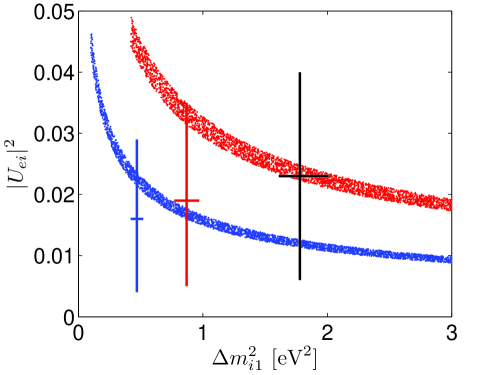
Figure 1: The allowed ranges of $|U_{e4}|^{2}-\Delta m^{2}_{41}$ (blue) and $|U_{e5}|^{2}-\Delta m^{2}_{51}$ (red) in the inverted ordering, requiring that the oscillation parameters lie in their currently allowed 2$\sigma$ ranges. The blue and red vertical and horizontal error bars indicate the allowed $2\sigma$ range for the $3+2$ mass and mixing parameters from Ref. Kopp et al. (2011), their intersection is the best-fit point. The black errors bars are for the $3+1$ case from Ref. Kopp et al. (2011), to be discussed in scenario II in Sect. III.3.2.

The effect of higher-order operators on the active-sterile mixing is very small. Switching on $w^{\prime}_{1}$ gives $|U_{e5}|^{2}\simeq{\cal O}(r_{1}^{2})\,\epsilon_{2}^{2}$ in the NO [cf. Eq. (37)], which will still not give sufficient mixing to explain the data. In the IO case, $|U_{e5}|^{2}\simeq 4[1+{\cal O}(r_{1})]\epsilon_{2}^{2}$, so the small correction term makes little difference. Indeed, the allowed ranges illustrated in Fig. 1 already include the effects of higher-order operators. One observes that the desired active-sterile mixing can indeed be achieved in the IO case.

In what regards active neutrino mixing, deviations from TBM come from both NLO seesaw terms ($\propto\epsilon_{i}$) and higher-order operators ($\propto y^{\prime}_{2},y^{\prime}_{3},w^{\prime}_{1},y^{\prime}_{\mu},y^{\prime}_{\tau}$). If we only consider higher-order corrections in the neutrino sector for simplicity, i.e. the $y^{\prime}_{2,3}$ and $w_{1}^{\prime}$ terms in Eqs. (A-5) and (A-8) respectively, then from Eqs. (37) and (38) only $U_{\mu 3}\propto\epsilon_{2}$ receives visible corrections in the NO, since $\epsilon_{1}$ and the product $\sigma^{N}_{+}R$ are both small. However, the higher-order terms related to the product $\sigma^{I}_{+}G$ lead to sizable corrections to $|U_{e2}|^{2}$ in the IO case; $|U_{e2}|$ could be enhanced or reduced depending on the signs and magnitudes of $y^{\prime}_{2,3}$ and $w_{1}^{\prime}$. In addition, non-zero $\theta_{13}$ can be obtained from the charged lepton corrections, as discussed in Sect. III.2 above.

III.3.2 Scenario II: split seesaw with both eV-scale and heavy right-handed neutrinos

We have shown that it is possible to get either normal or inverted ordering by choosing the alignment of the flavon VEV $\langle\varphi^{\prime\prime}\rangle$ correctly [cf. Eqs. (18) and (26)]. In this case we now assign different FN charges to the two seesaw right-handed neutrinos, so that there are four distinct possibilities, depending on the mass ordering of active neutrinos and which sterile neutrino ($\nu_{2}^{c}$ or $\nu_{3}^{c}$) is chosen as the heavy one. One can then use a two-stage seesaw, by integrating out the heavy sterile neutrino first and then applying the seesaw formula again. With the assignments $F_{1}=9$, $F_{2}=10\,(0)$ and $F_{3}=0\,(10)$ the sterile neutrino $\nu_{3}^{c}$ ($\nu_{2}^{c}$) has a mass in the $10^{11}$ GeV range, and is integrated out first, whereas $\nu_{2}^{c}$ ($\nu_{3}^{c}$) is at the eV scale. The third (second) column of $M_{D}$ is then used in the seesaw formula, leading to a $3\times 3$ effective neutrino mass matrix of rank 1 that gives one of the active neutrinos masses. The full $4\times 4$ mass matrix in the basis $(\nu_{e},\nu_{\mu},\nu_{\tau},\nu^{c}_{2(3)})$ leads to mixing between the active sector and the remaining eV-scale sterile neutrino $\nu^{c}_{2}$ ($\nu^{c}_{3}$). Here one can apply the method and formulae outlined in Sect. III.1, except that one has a $4\times 4$ mixing matrix, which can simply be obtained from the formulae in Eqs. (22) and (28) by removing the relevant row and column.

• Case IIA: $\nu_{3}^{c}$ heavy, ($F_{3}$ = 0), $\nu^{c}_{2}$ light ($F_{2}$ = 10)
  In this case one removes the fifth row and fifth column of $U_{\nu}$ in Eqs. (22) and (28), giving the same $4\times 4$ mixing matrix in both mass orderings, and the matrix elements $|U_{e5}|^{2}$ and $|U_{\mu 5}|^{2}$ are zero. The light neutrino mass eigenvalues $m_{i}$ ($i=1,2,3,4$) are given by the expressions in Eqs. (A-17) and (A-19) with $\epsilon_{2}$ set to zero; the heavy neutrino has the mass $M_{3}=w_{3}u^{\prime\prime}$. It is the small value of $F_{3}$ that leads to $\epsilon_{2}\simeq 0$ [Eq. (23)], so that $m_{3}$ (or $m_{1}$) does not receive any higher-order corrections, as this mass originates from the high-scale of $M_{3}$, whose FN charge “cancelled” in the leading order seesaw formula. Although in our example we have $F_{3}=0$, so that $M_{3}\simeq 10^{11}$ GeV, even with $F_{3}=5$ and $M_{3}\simeq 10$ GeV, one has $\epsilon_{2}\simeq 10^{-6}$ (see scenario III), so that NLO corrections would still be under control.

  The FN charge $F_{2}=10$ of the eV-scale neutrino gives corrections to $m_{2}$ and $m_{4}$, via $\epsilon_{1}\simeq 0.1$. With order one Yukawas and values for the VEVs as before, $M_{3}$ lies around $10^{11}$ GeV. The effective mass in $0\nu\beta\beta$ is given by the $(1,1)$ element of the $4\times 4$ mass matrix, which, at leading order, is

  $$\langle m_{ee}\rangle^{({\rm NO})}=0\,,\quad\langle m_{ee}\rangle^{({\rm IO})}=\left|\frac{2m^{(0)}_{1}}{3}\right|=\frac{2\sqrt{\Delta m_{\rm A}^{2}}}{3}\simeq 0.032~{}{\rm eV}\,.$$ (42)

  Here one can see that the contribution of the light neutrino of mass $m^{(0)}_{2}$ has cancelled with that of the light sterile neutrino $\nu^{c}_{2}$, in both mass orderings. Note again that this is different from the usually discussed effects of sterile neutrinos in $0\nu\beta\beta$. The effective mass is zero in the NO since at leading order, $U_{e3}=0$. A non-zero value of $U_{e3}$ would give a very small contribution to the effective mass in the NO, and a completely negligible one in the IO.

• Case IIB: $\nu_{2}^{c}$ heavy ($F_{2}$ = 0), $\nu^{c}_{3}$ light ($F_{3}$ = 10)
  Here the mixing matrix is found by removing the fourth row and column of Eqs. (22) and (28), so that the matrix elements in Eqs. (37) and (38) can be relabelled $|U_{e5}|^{2}\rightarrow|U_{e4}|^{2}$ and $|U_{\mu 5}|^{2}\rightarrow|U_{\mu 4}|^{2}$. The light neutrino mass eigenvalues $m_{i}$ ($i=1,2,3,4$) are now found by setting $\epsilon_{1}$ to zero in Eqs. (A-17) and (A-19), with the relabelling $m_{5}\rightarrow m_{4}$; the heavy neutrino has the mass $M_{2}=w_{2}u^{\prime}$. The roles of the sterile neutrinos are now swapped, and $M_{2}$ is situated at the $10^{11}$ GeV scale. The effective mass at leading order is

  $$\langle m_{ee}\rangle^{({\rm NO})} = \left|\frac{m^{(0)}_{2}}{3}\right|=\frac{\sqrt{\Delta m_{\rm S}^{2}}}{3}\simeq 0.0029~{}{\rm eV}\;,$$

  $$\langle m_{ee}\rangle^{({\rm IO})} = \left|\frac{m^{(0)}_{2}}{3}\right|\simeq\frac{\sqrt{\Delta m_{\rm A}^{2}}}{3}\simeq 0.016~{}{\rm eV}\;;$$ (43)

  in this case the contribution of $m^{(0)}_{3}$ has cancelled. Again, corrections to the mixing angles give very small corrections to the effective mass.

In both cases IIA and IIB one could potentially explain the reactor anomaly in the framework of $3+1$ neutrino mixing Kopp et al. (2011); Giunti and Laveder (2011c), with $|U_{e4}|^{2}\simeq[1+{\cal O}(r_{1})]\,\epsilon_{1}^{2}$ in case IIA and $|U_{e4}|^{2}\simeq 4[1+{\cal O}(r_{1})]\epsilon_{2}^{2}$ in the IO in case B. Once again only the IO fits the data: the allowed ranges in the mass-mixing plane for the IO in case IIA (IIB) are shown by the blue (red) points in Fig. 1. One can see that the best-fit point (the black cross) from Ref. Kopp et al. (2011) is compatible with case IIB. Finally, the effects of higher-order operators on both active-sterile mixing and active mixing are the same as in scenario I, except that one should switch off the effect of $\epsilon_{2}$ ($\epsilon_{1}$) in case IIA (IIB).

III.3.3 Scenario III: two heavy right-handed neutrinos

In this case we take $F_{1}=9$, $F_{2,3}=5$, so that one can estimate that the $\epsilon_{i}\simeq 10^{-6}$ ($i=1,2$) are dramatically suppressed, and the NLO seesaw terms in Eqs. (22) and (28) can be safely neglected. The $3\times 3$ effective neutrino mass matrix is given by Eq. (3), with $M_{D}$ defined in Eqs. (20) or (27) and $M_{R}$ from Eq. (21); the active neutrino masses are simply given by the leading order masses $m_{i}^{(0)}$. The heavy neutrinos have masses $M_{2}=w_{2}u^{\prime}\lambda^{10}$ and $M_{3}=w_{3}u^{\prime\prime}\lambda^{10}$. Without the effect of the $\epsilon_{i}$ terms, the only modifications to the TBM pattern come from the higher-order operators in Sect. III.2.

The two heavy right-handed neutrinos that participate in the seesaw formula have masses around 5 GeV, assuming order one Yukawas and the usual values of the VEVs. Note that one could set $w_{2}=w_{3}$ to obtain degenerate right-handed neutrinos $M_{2}=M_{3}$. The choice of degenerate sterile neutrinos in the few GeV regime would correspond to the $\nu$MSM paradigm, in which no new scales between the SM and the Planck scale are assumed. Baryogenesis then proceeds via oscillations between $\nu_{2}^{c}$ and $\nu_{3}^{c}$, which need to be sufficiently degenerate $\left(|M_{2}-M_{3}|/M_{2}\simeq 10^{-6}\right)$ to give the correct baryon asymmetry Canetti and Shaposhnikov (2010).

If we choose $F_{2,3}=0$ instead, then $M_{2,3}\simeq 10^{11}$ GeV, so that the CP-violating decay of right-handed neutrinos could explain the matter dominated Universe via thermal leptogenesis. The required CP violation may originate from complex Yukawa couplings. We further note that, similar to the ordinary type I seesaw, neutrinoless double beta decay is allowed, and the right-handed neutrinos play no role in this process since their contribution $\sum_{i=2,3}\theta_{i}^{2}/M_{i}$ is strongly suppressed by the inverse of their mass. Explicitly, at leading order the effective mass from the $(1,1)$ entry of Eq. (3) is

$$\langle m_{ee}\rangle^{({\rm NO})} =\left|\frac{m^{(0)}_{2}}{3}\right|=\frac{\sqrt{\Delta m_{\rm S}^{2}}}{3}\simeq 0.0029~{}{\rm eV}\;,$$ (44)

$$\langle m_{ee}\rangle^{({\rm IO})} =\left|\frac{2m^{(0)}_{1}}{3}+\frac{m^{(0)}_{2}}{3}\right|\simeq\sqrt{\Delta m_{\rm A}^{2}}\simeq 0.049~{}{\rm eV}\;,$$ (45)

where the mass eigenvalues are real. If $m^{(0)}_{1}$ and $m^{(0)}_{2}$ are complex, the IO case becomes $\langle m_{ee}\rangle^{({\rm IO})}\mathrel{\hbox to0.0pt{\raise 2.20013pt\hbox{$<$}\hss}{\lower 2.20013pt\hbox{$\sim$}}}\sqrt{\Delta m_{\rm A}^{2}}$. Corrections from higher order terms are again small.

IV An effective theory approach

In this section we recast the idea presented in Ref. Barry et al. (2011), this time in the context of keV sterile neutrino WDM rather than eV-scale sterile neutrinos. A popular flavor symmetry model, which predicts TBM and is based on the group $A_{4}$, is modified in order to accommodate a keV sterile neutrino. Unlike the seesaw model, neutrinos get mass from effective operators and only one sterile state is introduced. We also extend the discussion to include the effects of higher-order operators.

IV.1 $A_{4}$ symmetry with one keV sterile neutrino

The Altarelli-Feruglio (AF) $A_{4}$ neutrino mass model Altarelli and Feruglio (2005) is well known, and at leading order gives exact TBM for the lepton flavor mixing matrix. The original AF model includes three sets of flavon fields $\varphi$, $\varphi^{\prime}$ and $\xi$ in addition to the SM particle content. We add an additional sterile neutrino transforming as a singlet under $A_{4}$ and $Z_{3}$, with the $U(1)_{\rm FN}$ charge of $F_{s}=8$. The relevant particle assignments are summarized in Table 3.

Table 3: Particle assignments of the $A_{4}$ model, modified from Ref. Altarelli and Feruglio (2005) to include a sterile neutrino $\nu_{s}$. The additional $Z_{3}$ symmetry decouples the charged lepton and neutrino sectors; the $U(1)_{\rm FN}$ charge generates the hierarchy of charged lepton masses and regulates the scale of the sterile state.

Field	$L$	$e^{c}$	$\mu^{c}$	$\tau^{c}$	$h_{u,d}$	$\varphi$	$\varphi^{\prime}$	$\xi$	$\Theta$	$\nu_{s}$
$SU(2)_{L}$	$2$	$1$	$1$	$1$	$2$	$1$	$1$	$1$	$1$	$1$
$A_{4}$	$\underline{3}$	$\underline{1}$	$\underline{1}^{\prime\prime}$	$\underline{1}^{\prime}$	$\underline{1}$	$\underline{3}$	$\underline{3}$	$\underline{1}$	$\underline{1}$	$\underline{1}$
$Z_{3}$	$\omega$	$\omega^{2}$	$\omega^{2}$	$\omega^{2}$	$1$	$1$	$\omega$	$\omega$	$1$	$1$
$U(1)_{\rm FN}$	-	$4$	$2$	$0$	-	-	-	-	$-1$	$8$

As discussed in Ref. Barry et al. (2011), at leading order the Yukawa couplings for the lepton sector read

$$-{\cal L}_{\rm Y} = \frac{y_{e}}{\Lambda}\lambda^{4}\left(\varphi Lh_{d}\right)e^{c}+\frac{y_{\mu}}{\Lambda}\lambda^{2}\left(\varphi Lh_{d}\right)^{\prime}\mu^{c}+\frac{y_{\mu}}{\Lambda}\left(\varphi Lh_{d}\right)^{\prime\prime}\tau^{c}+\frac{x_{a}}{\Lambda^{2}}\xi(Lh_{u}Lh_{u})+\frac{x_{d}}{\Lambda^{2}}(\varphi^{\prime}Lh_{u}Lh_{u})$$ (46)

$$+\frac{x_{e}}{\Lambda^{2}}\lambda^{8}\xi(\varphi^{\prime}Lh_{u})\nu_{s}+\frac{x_{f}}{\Lambda^{2}}\lambda^{8}(\varphi^{\prime}\varphi^{\prime}Lh_{u})\nu_{s}+m_{s}\lambda^{16}\nu^{c}_{s}\nu^{c}_{s}+{\rm h.c.},$$

where $m_{s}$ is a bare Majorana mass. Note that the $A_{4}$ invariant dimension-5 operator $\frac{1}{\Lambda}\lambda^{8}(\varphi^{\prime}Lh_{u})\nu_{s}$ is not invariant under the $Z_{3}$ symmetry. With the following vacuum alignments (as in the AF model)

$$\langle\varphi\rangle=(v,0,0)\;,\quad\langle\varphi^{\prime}\rangle=(v^{\prime},v^{\prime},v^{\prime})\;,\quad\langle\xi\rangle=u\;,\quad\langle h_{u,d}\rangle=v_{u,d}\;,$$ (47)

the charged lepton mass matrix is diagonal [cf. Eq. (14)], and the full $4\times 4$ neutrino mass matrix is

$$M^{4\times 4}_{\nu}=\begin{pmatrix}a+\frac{2d}{3}&-\frac{d}{3}&-\frac{d}{3}&e\\ \cdot&\frac{2d}{3}&a-\frac{d}{3}&e\\ \cdot&\cdot&\frac{2d}{3}&e\\ \cdot&\cdot&\cdot&m_{s}\end{pmatrix},$$ (48)

where $a=2x_{a}\frac{uv_{u}^{2}}{\Lambda^{2}}$, $d=2x_{d}\frac{v^{\prime}v_{u}^{2}}{\Lambda^{2}}$ and $e=\sqrt{2}x_{e}\lambda^{8}\frac{uv^{\prime}v_{u}}{\Lambda^{2}}$ have dimensions of mass. The first three elements of the fourth row of $M^{4\times 4}_{\nu}$ are identical because of the VEV alignment $\langle\varphi^{\prime}\rangle=(v^{\prime},v^{\prime},v^{\prime})$, which was necessary to generate TBM in the three-neutrino case; this alignment combined with the $A_{4}$ multiplication rules causes the term proportional to $x_{f}$ in Eq. (46) to vanish.

If one assumes that $a<m_{s}$ and expands to second order in the small ratio $e/m_{s}$, the mixing matrix diagonalizing $M^{4\times 4}_{\nu}$ in Eq. (48) is Barry et al. (2011)

$$U\simeq\begin{pmatrix}\frac{2}{\sqrt{6}}&\frac{1}{\sqrt{3}}&0&0\\ -\frac{1}{\sqrt{6}}&\frac{1}{\sqrt{3}}&-\frac{1}{\sqrt{2}}&0\\ -\frac{1}{\sqrt{6}}&\frac{1}{\sqrt{3}}&\frac{1}{\sqrt{2}}&0\\ 0&0&0&1\end{pmatrix}+\begin{pmatrix}0&0&0&\frac{e}{m_{s}}\\ 0&0&0&\frac{e}{m_{s}}\\ 0&0&0&\frac{e}{m_{s}}\\ 0&-\frac{\sqrt{3}e}{m_{s}}&0&0\end{pmatrix}+{\cal O}\left(\frac{e^{2}}{m_{s}^{2}}\right),$$ (49)

with the eigenvalues

$$m_{1}=a+d\,,~{}~{}m_{2}=a-\frac{3e^{2}}{m_{s}}\,,~{}~{}m_{3}=-a+d\,,~{}~{}m_{4}=m_{s}+\frac{3e^{2}}{m_{s}}\,.$$ (50)

As we will see, the chosen FN charge forces $m_{s}$ to be at the desired keV scale and sets the magnitude of active-sterile mixing, $e/m_{s}={\cal O}(10^{-4})$. This means that the “seesaw contribution” ($\propto e^{2}/m_{s}$) to $m_{2}$ in Eq. (50) is negligible.

IV.2 Estimation of the mass scales and active-sterile mixing

In order to examine the viability of the model we provide a rough numerical example. As discussed in the original AF model Altarelli and Feruglio (2005), we assume that $(i)$ the Yukawa couplings $y$ and $x$ remain in a perturbative regime; $(ii)$ the flavon VEVs are smaller than the cut-off scale and $(iii)$ all flavon VEVs fall in approximately the same range, and obtain the following relation constraining the flavon VEVs:

$$0.004<\frac{u}{\Lambda}\approx\frac{v^{\prime}}{\Lambda}\approx\frac{v}{\Lambda}<1\,,$$ (51)

with the cut-off scale $\Lambda$ ranging between $10^{12}$ and $10^{15}$ GeV. We would like to suppress the mass of the keV neutrino, while at the same time keep its mixing small enough and satisfy the conditions in Eq. (51). By choosing the FN charge of $\nu_{s}$ (i.e. $F_{s}=8$) and the mass scales

$$u\simeq v^{\prime}\simeq 10^{10}~{}{\rm GeV}\;,\quad v\simeq 10^{11}~{}{\rm GeV}\;,\quad\Lambda\simeq 10^{12}~{}{\rm GeV}\;,$$

$$v_{u,d}\simeq 10^{2}~{}{\rm GeV}\;,\quad\langle\Theta\rangle\simeq 10^{11}~{}{\rm GeV}\;,$$ (52)

which means that $\lambda=\langle\Theta\rangle/\Lambda\simeq 0.1$, one obtains

$$\begin{array}[]{c}\displaystyle a\simeq d\simeq 0.1\left(\frac{u}{10^{10}~{}{\rm GeV}}\right)\left(\frac{v_{u}}{10^{2}~{}{\rm GeV}}\right)^{2}\left(\frac{10^{12}~{}{\rm GeV}}{\Lambda}\right)^{2}\ {\rm eV}\,,\\[5.69054pt] \displaystyle e\simeq 0.1\left(\frac{\lambda}{10^{-1}}\right)^{8}\left(\frac{u}{10^{10}~{}{\rm GeV}}\right)\left(\frac{v^{\prime}}{10^{10}~{}{\rm GeV}}\right)\left(\frac{v_{u}}{10^{2}~{}{\rm GeV}}\right)\left(\frac{10^{12}~{}{\rm GeV}}{\Lambda}\right)^{2}\ {\rm eV}\,,\end{array}$$ (53)

with the assumption that the Yukawa couplings $x_{a,d,e}$ are of order 1.

The Majorana mass term $m_{s}\nu^{c}_{s}\nu^{c}_{s}$ is doubly suppressed by the $U(1)_{\rm FN}$ charge. There are additional terms that can give a contribution to this mass in addition to the bare term. From the particle assignments in Table 3, the leading order contribution to $m_{s}$ reads

$$\left(\frac{x_{s}}{\Lambda}\varphi\varphi\right)\lambda^{16}\nu^{c}_{s}\nu^{c}_{s}\Longrightarrow\left({x_{s}}\frac{v^{2}}{\Lambda}\right)\lambda^{16}\,,$$ (54)

so that these terms are suppressed by $\lambda^{16}$, and the resulting Majorana mass can be of order keV:

$$m_{s}\simeq\left(\frac{\lambda}{10^{-1}}\right)^{16}\left(\frac{v}{10^{11}~{}{\rm GeV}}\right)^{2}\left(\frac{10^{12}~{}{\rm GeV}}{\Lambda}\right)\ {\rm keV}\,.$$ (55)

The active-sterile mixing is given by

$$\theta_{s}=\frac{e}{m_{s}}\simeq 10^{-4}\,,$$ (56)

corresponding to $\sin^{2}\!\theta_{s}\simeq 10^{-8}$, in accordance with the astrophysical constraints discussed in Sect. II. It should also be noticed that in this model the charged lepton masses are

$$m_{\alpha}=y_{\alpha}v_{d}\frac{v}{\Lambda}\lambda^{F_{\alpha}}\simeq 10\left(\frac{v_{d}}{10^{2}~{}{\rm GeV}}\right)\left(\frac{v}{10^{11}~{}{\rm GeV}}\right)\left(\frac{10^{12}~{}{\rm GeV}}{\Lambda}\right)\left(\frac{\lambda}{10^{-1}}\right)^{F_{\alpha}}\ {\rm GeV}\,,$$ (57)

so that we get the correct mass spectrum with the FN charges ($F_{\alpha}$) of 4, 2 and 0 for $e^{c}$, $\mu^{c}$ and $\tau^{c}$, respectively [assuming $y_{\alpha}\mathrel{\hbox to0.0pt{\raise 2.20013pt\hbox{$<$}\hss}{\lower 2.20013pt\hbox{$\sim$}}}{\cal O}(1)$].

IV.3 Higher-order corrections and non-zero $\theta_{13}$

One may also wonder if higher-order terms could lead to significant corrections to the lepton flavor mixing and neutrino masses so as to generate a non-zero $\theta_{13}$, as suggested by the T2K experiment. In general, both the neutrino and charged lepton mass matrices receive higher-order corrections, suppressed by additional powers of the cutoff scale $\Lambda$; those are the only type of corrections that we consider here.

In the charged lepton sector, the NLO corrections to $M_{\ell}$ come from terms like

$$\frac{1}{\Lambda^{2}}\left[y^{\prime}_{e}\lambda^{4}\left(\varphi\varphi Lh_{d}\right)e^{c}+y^{\prime}_{\mu}\lambda^{2}\left(\varphi\varphi Lh_{d}\right)^{\prime}\mu^{c}+y^{\prime}_{\tau}\left(\varphi\varphi Lh_{d}\right)^{\prime\prime}\tau^{c}\right],$$ (58)

which however replicate the leading order patterns, as in the seesaw model (see Appendix A.1). The NLO corrections to $M_{\ell}$ can thus be simply absorbed into the coefficients $y_{\alpha}$.

As for the sterile neutrino, the NLO corrections to $m_{s}$ are given by

$$\left(\frac{x_{s^{\prime}}}{\Lambda^{2}}\xi\xi\xi+\frac{x_{s^{\prime\prime}}}{\Lambda^{2}}(\varphi^{\prime}\varphi^{\prime})\xi\right)\lambda^{16}\nu^{c}_{s}\nu^{c}_{s}\Longrightarrow\left(x_{s^{\prime}}\frac{u^{3}}{\Lambda^{2}}+x_{s^{\prime\prime}}\frac{3v^{\prime 2}u}{\Lambda^{2}}\right)\lambda^{16}\,;$$ (59)

in this case the contributions in Eq. (59) are of order $10^{-4}$ keV, and do not affect the scale of $m_{s}$ significantly. Note that the term $\frac{x_{s^{\prime\prime}}}{\Lambda^{2}}\lambda^{16}(\varphi^{\prime}\varphi^{\prime}\varphi^{\prime})\nu_{s}^{c}\nu_{s}^{c}$ is in principle also allowed, but vanishes after $A_{4}$ symmetry breaking, just like the $x_{f}$ term in Eq. (46). NLO corrections to the $e$ parameter come from terms like

$$\frac{x^{\prime}_{e}}{\Lambda^{3}}\lambda^{8}\xi(\varphi^{\prime}\varphi Lh_{u})\nu_{s}\,,$$ (60)

which lead to

$$e^{\prime}\simeq 0.01\left(\frac{\lambda}{10^{-1}}\right)^{8}\left(\frac{u\,v^{\prime}}{(10^{10}~{}{\rm GeV})^{2}}\right)\left(\frac{v}{10^{11}~{}{\rm GeV}}\right)\left(\frac{v_{u}}{10^{2}~{}{\rm GeV}}\right)\left(\frac{10^{12}~{}{\rm GeV}}{\Lambda}\right)^{3}\ {\rm eV}\;,$$ (61)

indicating again that the active-sterile mixing is hardly affected.

The higher-order operators contributing to light neutrino masses are of order $1/\Lambda^{3}$. There exist only three such terms that cannot be absorbed by a redefinition of the parameters $a$ and $b$ Altarelli and Feruglio (2006), i.e.

$$\frac{x_{1}}{\Lambda^{3}}(\varphi\varphi^{\prime})^{\prime}(Lh_{u}Lh_{u})^{\prime\prime}\;,\quad\frac{x_{2}}{\Lambda^{3}}(\varphi\varphi^{\prime})^{\prime\prime}(Lh_{u}Lh_{u})^{\prime}\;,\quad{\rm and}\quad\frac{x_{3}}{\Lambda^{3}}\xi(\varphi Lh_{u}Lh_{u})\;,$$ (62)

so that the light neutrino mass matrix is modified to

$$M_{\nu}=M^{(0)}_{\nu}+M^{(1)}_{\nu}=\begin{pmatrix}a+\frac{2d}{3}&-\frac{d}{3}&-\frac{d}{3}\\ \cdot&\frac{2d}{3}&a-\frac{d}{3}\\ \cdot&\cdot&\frac{2d}{3}\end{pmatrix}+\begin{pmatrix}\frac{2}{3}\eta_{3}&\eta_{2}&\eta_{1}\\ \cdot&\eta_{1}&-\frac{1}{3}\eta_{3}\\ \cdot&\cdot&\eta_{2}\end{pmatrix},$$ (63)

where $\eta_{1}=2x_{1}\frac{vv^{\prime}v^{2}_{u}}{\Lambda^{3}}$, $\eta_{2}=2x_{2}\frac{vv^{\prime}v^{2}_{u}}{\Lambda^{3}}$ and $\eta_{3}=2x_{3}\frac{uvv^{2}_{u}}{\Lambda^{3}}$. For ${\cal O}(1)$ Yukawa couplings, one can estimate that

$$\eta_{i}\simeq 0.01\left(\frac{v}{10^{11}~{}{\rm GeV}}\right)\left(\frac{v^{\prime}}{10^{10}~{}{\rm GeV}}\right)\left(\frac{v_{u}}{10^{2}~{}{\rm GeV}}\right)^{2}\left(\frac{10^{12}~{}{\rm GeV}}{\Lambda}\right)^{3}\ {\rm eV}\,.$$ (64)

As a result, the NLO terms may lead to visible modifications to the TBM pattern, in particular to $\theta_{13}$, but on the other hand do not entirely spoil the leading order picture, since one always has enough parameters to fit the data. Keeping only first order terms in $\eta_{i}$, one obtains

$$m_{1} \simeq a+b-\frac{1}{2}\left(\eta_{1}+\eta_{2}\right)+\frac{1}{3}\eta_{3}\;,$$

$$m_{2} \simeq a+\eta_{1}+\eta_{2}\;,$$ (65)

$$m_{3} \simeq -a+b+\frac{1}{2}\left(\eta_{1}+\eta_{2}\right)+\frac{1}{3}\eta_{3}\;,$$

together with the mixing angles

$$\sin^{2}\!\theta_{13} \simeq \frac{(\eta_{1}-\eta_{2})^{2}}{8a^{2}}\;,$$

$$\sin^{2}\!\theta_{12} \simeq \frac{1}{3}\left(1-\frac{2\eta_{3}}{3b}\right),$$ (66)

$$\sin^{2}\!\theta_{23} \simeq \frac{1}{2}\left(1-\frac{\eta_{1}-\eta_{2}}{4a}\right).$$

As one numerical example, we take $\eta_{2}=-\eta_{1}=0.1a$ and $\eta_{3}=0.1b$, and obtain $\sin^{2}\theta_{13}\simeq 0.005$, which is compatible with the current global-fit data at $2\sigma$ C.L. In addition, $\sin^{2}\theta_{23}\simeq 0.53$ and $\sin^{2}\theta_{12}\simeq 0.31$ are predicted, in good agreement with their best-fit values Schwetz et al. (2011b, a).

V Conclusion

The addition of sterile right-handed neutrinos to the SM is a natural way to explain light active neutrino masses via the seesaw mechanism. This works even if the scale of the sterile neutrinos is not equal to its “natural value” of $10^{10}$ to $10^{15}$ GeV, as long as the Dirac mass matrix can also be suppressed such that $M_{D}^{2}/M_{R}$ is small. At the same time, several observations point to sterile neutrinos at the keV and eV scales. Therefore we have attempted, as a proof of principle, to construct a seesaw model for neutrino mass and lepton mixing that can provide a common framework for all these issues.

Starting from a flavor symmetry model based on the tetrahedral group $A_{4}$, we described different ways to introduce sterile neutrinos, using the seesaw mechanism (and also an effective theory approach). In both cases the Froggatt-Nielsen (FN) mechanism is used to suppress the masses of the right-handed neutrinos. We stress that its presence in flavor symmetry models can be considered necessary in order to generate the observed strong hierarchy in the charged lepton sector. In fact, we utilize the very same FN for both the charged lepton masses and the right-handed neutrinos.

In the seesaw model we studied different possible spectra in the sterile sector: once the keV WDM neutrino is decoupled one can have the remaining two neutrinos at the eV scale or at a high scale (in our example at either 10 GeV or close to the flavor symmetry breaking scale of $\simeq 10^{11}$ GeV). In each case there are distinct phenomenological consequences, both for neutrino mass and neutrinoless double beta decay. In particular, NLO corrections to the seesaw formula need to be taken into account when the sterile neutrinos are at the eV scale.

Motivated by the recent indications for nonzero $\theta_{13}$ in the T2K experiment, we examined the effect of higher-order terms in both the seesaw model and the effective theory. In general active neutrino mixing angles will receive corrections of the same order. We highlighted the fact that active-sterile mixing is stable in any seesaw model, being defined as the ratio of two large scales.

Although one can explain both eV-scale and keV-scale sterile neutrinos in a single framework, it is not possible to have viable WDM, eV-scale neutrinos and heavy neutrinos for leptogenesis in a model containing three right-handed neutrinos. However, we emphasize the point that if one departs from the common theoretical prejudice of right-handed neutrinos residing at around the Grand Unification scale, various interesting model building options can arise. Further experimental data in the years to come will put the presence of sterile neutrinos at the eV and/or keV scale/s to the test, thus determining whether it is indeed a useful enterprise to further pursue this avenue of research.

Appendix A Corrections from higher-order operators in the seesaw model

Here we give details of the procedure followed to calculate corrections to the lepton mixing matrix in the presence of higher-order operators, which affect $M_{\ell}$, $M_{D}$ and $M_{R}$. We only take into account corrections of relative order $r_{1}\simeq 0.1$ [cf. Eq. (34)]. Explicit expressions for the corrected neutrino mass eigenvalues are also reported.

A.1 Charged lepton sector

The corrections to $M_{\ell}$ from dimension-six operators come from coupling a second $A_{4}$ triplet or an $A_{4}$ singlet to each mass term. The addition of the flavon $\varphi$ replicates the leading order pattern, since the triplet from the product $(\varphi\varphi)_{3}$ has a VEV in the same direction as $\varphi$ Altarelli and Feruglio (2006). Terms with the additional singlet $\xi^{\prime\prime}$ also leave the structure of the mass matrix unchanged, but the additional terms

$$\frac{y^{\prime}_{e}}{\Lambda^{2}}\lambda^{3}\xi(\varphi^{\prime}Lh_{d})e^{c}\ ,\frac{y^{\prime\prime}_{e}}{\Lambda^{2}}\lambda^{3}\xi^{\prime}(\varphi^{\prime\prime}Lh_{d})^{\prime\prime}e^{c}\quad{\rm and}\quad\frac{y^{\prime\prime\prime}_{e}}{\Lambda^{2}}\lambda^{3}(\varphi^{\prime}\varphi^{\prime\prime}Lh_{d})e^{c}$$ (A-1)

are also present, for all three flavors. The first term gives the largest NLO contribution, i.e.

$$\delta M^{(1)}_{\ell}=\frac{v_{d}uv^{\prime}}{\Lambda^{2}}\begin{pmatrix}y^{\prime}_{e}\lambda^{3}&y^{\prime}_{\mu}\lambda&y^{\prime}_{\tau}\\ y^{\prime}_{e}\lambda^{3}&y^{\prime}_{\mu}\lambda&y^{\prime}_{\tau}\\ y^{\prime}_{e}\lambda^{3}&y^{\prime}_{\mu}\lambda&y^{\prime}_{\tau}\end{pmatrix},$$ (A-2)

of relative order $r_{1}\simeq 0.1$. The matrix diagonalizing $(M_{\ell}+\delta M^{(1)}_{\ell})(M_{\ell}+\delta M^{(1)}_{\ell})^{\dagger}$ can be approximated by

$$V_{\ell}\simeq\begin{pmatrix}1&\frac{y^{\prime}_{\mu}}{y_{\mu}}r_{1}&\frac{y^{\prime}_{\tau}}{y_{\tau}}r_{1}\\[4.2679pt] -\frac{y^{\prime}_{\mu}}{y_{\mu}}r_{1}&1&\frac{y^{\prime}_{\tau}}{y_{\tau}}r_{1}\\[4.2679pt] -\frac{y^{\prime}_{\tau}}{y_{\tau}}r_{1}&-\frac{y^{\prime}_{\tau}}{y_{\tau}}r_{1}&1\end{pmatrix}+{\cal O}(r_{1}^{2},\lambda^{2})\,,$$ (A-3)

and the charged lepton masses become

$$m^{\prime}_{\alpha}=(y_{\alpha}+y^{\prime}_{\alpha}r_{1})\frac{v_{d}v}{\Lambda}\lambda^{F_{\alpha}},\qquad(\alpha=e,\mu,\tau),$$ (A-4)

which amounts to a rescaling of Yukawa couplings.

A.2 Neutrino sector

Similarly to $M_{\ell}$, corrections to $M_{D}$ from adding the singlet $\xi^{\prime\prime}$ retain the leading order form, but there are also several terms with two triplet flavons. The latter are all suppressed by $r_{2}\simeq 0.01$ and can be safely neglected. Of the nine different invariant dimension-six operators with one triplet and one singlet flavon, there are three of relative order $r_{1}\simeq 0.1$, namely

$$\frac{y^{\prime}_{1}}{\Lambda^{2}}\lambda^{F_{1}}\xi(\varphi^{\prime}Lh_{u})\nu_{1}^{c}+\frac{y^{\prime}_{2}}{\Lambda^{2}}\lambda^{F_{2}}\xi(\varphi^{\prime\prime}Lh_{u})^{\prime\prime}\nu_{2}^{c}+\frac{y^{\prime}_{3}}{\Lambda^{2}}\lambda^{F_{3}}\xi(\varphi Lh_{u})\nu_{3}^{c}\,,$$ (A-5)

leading to the corrections

$$\delta M_{D}^{(1N)}=\frac{v_{u}u}{\Lambda^{2}}\begin{pmatrix}y^{\prime}_{1}v^{\prime}&-y_{2}^{\prime}v^{\prime\prime}&y^{\prime}_{3}v\\ y^{\prime}_{1}v^{\prime}&y_{2}^{\prime}v^{\prime\prime}&0\\ y^{\prime}_{1}v^{\prime}&0&0\end{pmatrix}F\quad{\rm and}\quad\delta M_{D}^{(1I)}=\frac{v_{u}u}{\Lambda^{2}}\begin{pmatrix}y^{\prime}_{1}v^{\prime}&-y^{\prime}_{2}v^{\prime\prime}&y^{\prime}_{3}v\\ y^{\prime}_{1}v^{\prime}&-y_{2}^{\prime}v^{\prime\prime}&0\\ y^{\prime}_{1}v^{\prime}&2y^{\prime}_{2}v^{\prime\prime}&0\end{pmatrix}F\,,$$ (A-6)

in the normal and inverted ordering, respectively. Here the matrix of FN charges is

$$F={\rm diag}(\lambda^{F_{1}},\lambda^{F_{2}},\lambda^{F_{3}})\,.$$ (A-7)

The corrections to $M_{R}$ come from terms with two singlets and those with two triplets, e.g.

$$\frac{w^{\prime}_{1}}{\Lambda}\lambda^{F_{1}+F_{3}}\xi\xi\nu_{1}^{c}\nu_{3}^{c}+\ldots\quad{\rm and}\quad\frac{w^{\prime\prime}_{1}}{\Lambda}\lambda^{F_{1}+F_{3}}(\varphi\varphi^{\prime})\nu_{1}^{c}\nu_{3}^{c}+\ldots\,;$$ (A-8)

the singlet terms give the contribution

$$\delta M^{(1)}_{R}\propto\frac{1}{\Lambda}\begin{pmatrix}uu^{\prime\prime}\lambda^{2F_{1}}&0&uu\lambda^{F_{1}+F_{3}}\\ \cdot&u^{\prime}u^{\prime\prime}\lambda^{2F_{2}}&u^{\prime}u^{\prime}\lambda^{F_{2}+F_{3}}\\ \cdot&\cdot&u^{\prime\prime}u^{\prime\prime}\lambda^{2F_{3}}\end{pmatrix}\,,$$ (A-9)

whereas the triplet terms are all suppressed by $r_{2}\simeq 0.01$. Comparison of the LO and NLO terms shows that the large ratio $r_{1}\simeq 0.1$ only occurs in the $(1,3)$ element of $\delta M^{(1)}_{R}$, whereas the diagonal and $(2,3)$ elements receive small corrections of order $r_{2}\simeq 0.01$. Ignoring the latter, the new mass matrix is

$$M^{\prime}_{R}=M_{R}+\delta M^{(1)}_{R}=F\begin{pmatrix}w_{1}u&0&w^{\prime}_{1}ur_{1}\\ \cdot&w_{2}u^{\prime}&0\\ \cdot&\cdot&w_{3}u^{\prime\prime}\end{pmatrix}F\,.$$ (A-10)

It is convenient to factor out the FN charges here, since they do not appear in the leading order seesaw formula. However, as emphasized before, they will play a role when considering NLO seesaw terms. Expanding in the small ratios $r_{1}\simeq\frac{w_{3}u^{\prime\prime}}{w_{1}u}\simeq 0.1$, the matrix diagonalizing $M^{\prime}_{R}$ can be approximated as

$$V_{R}\simeq F^{-1}\begin{pmatrix}1&0&-\frac{w^{\prime}_{1}}{w_{1}}r_{1}\\ 0&1&0\\ \frac{w^{\prime}_{1}}{w_{1}}r_{1}&0&1\end{pmatrix}F+{\cal O}\left(\frac{w_{3}u^{\prime\prime}}{w_{1}u}r_{1},r_{1}^{2}\right),$$ (A-11)

with the mass eigenvalues

$$M^{\prime}_{1} =w_{1}u\lambda^{2F_{1}}\left(1+\frac{{w^{\prime}_{1}}^{2}}{w_{1}^{2}}r_{1}^{2}\right)\,,$$

$$M^{\prime}_{2} =w_{2}u^{\prime}\lambda^{2F_{2}}\,,$$ (A-12)

$$M^{\prime}_{3} =w_{3}u^{\prime\prime}\lambda^{2F_{3}}\left(1-\frac{{w^{\prime}_{1}}^{2}}{w_{1}^{2}}r_{1}^{2}\right).$$

This shows that corrections to the masses $M_{1,3}$ are suppressed by $r_{1}^{2}$, and the WDM candidate $\nu_{1}^{c}$ remains in the keV range.

The diagonalization matrix in Eq. (A-11) can be absorbed into $M_{D}$, so that the leading order neutrino mass matrix is

$$M^{\prime}_{\nu}=-M_{D}^{\prime}{\rm diag}({M^{\prime}_{1}}^{-1},{M^{\prime}_{2}}^{-1},{M^{\prime}_{3}}^{-1}){M_{D}^{\prime}}^{T}\,,$$ (A-13)

where $M_{D}^{\prime}=\left(M_{D}+\delta M_{D}^{(1)}\right)V^{*}_{R}$ and the FN charges have cancelled. The Dirac mass matrices in Eqs. (20) and (27) plus the corrections terms in Eq. (A-6) lead to

$${M^{\prime}_{D}}^{({\rm NO})} =\frac{v_{u}}{\Lambda}\begin{pmatrix}y_{1}v+y^{\prime}_{1}v^{\prime}r_{1}&y_{2}v^{\prime}-y^{\prime}_{2}v^{\prime\prime}r_{1}&\left(y^{\prime}_{3}v-y_{1}v\frac{w^{\prime}_{1}}{w_{1}}\right)r_{1}\\[5.69054pt] \left(y^{\prime}_{1}v^{\prime}-y_{3}v^{\prime\prime}\frac{w^{\prime}_{1}}{w_{1}}\right)r_{1}&y_{2}v^{\prime}+y^{\prime}_{2}v^{\prime\prime}r_{1}&-y_{3}v^{\prime\prime}\\[5.69054pt] \left(y^{\prime}_{1}v^{\prime}+y_{3}v^{\prime\prime}\frac{w^{\prime}_{1}}{w_{1}}\right)r_{1}&y_{2}v^{\prime}&y_{3}v^{\prime\prime}\end{pmatrix}F,$$

$${M^{\prime}_{D}}^{({\rm IO})} =\frac{v_{u}}{\Lambda}\begin{pmatrix}y_{1}v+\left(y^{\prime}_{1}v^{\prime}+2y_{3}v^{\prime\prime}\frac{w^{\prime}_{1}}{w_{1}}\right)r_{1}&y_{2}v^{\prime}-y^{\prime}_{2}v^{\prime\prime}r_{1}&2y_{3}v^{\prime\prime}+\left(y^{\prime}_{3}v-y_{1}v\frac{w^{\prime}_{1}}{w_{1}}\right)r_{1}\\[5.69054pt] \left(y^{\prime}_{1}v^{\prime}-y_{3}v^{\prime\prime}\frac{w^{\prime}_{1}}{w_{1}}\right)r_{1}&y_{2}v^{\prime}-y^{\prime}_{2}v^{\prime\prime}r_{1}&-y_{3}v^{\prime\prime}\\[5.69054pt] \left(y^{\prime}_{1}v^{\prime}-y_{3}v^{\prime\prime}\frac{w^{\prime}_{1}}{w_{1}}\right)r_{1}&y_{2}v^{\prime}+2y^{\prime}_{2}v^{\prime\prime}r_{1}&-y_{3}v^{\prime\prime}\end{pmatrix}F\,,$$ (A-14)

to first order in $r_{1}$, in the NO and IO, respectively. As shown explicitly in the main text, the dynamics of the right-handed sector are relatively unaffected: the new entries in the first column of the Dirac mass matrices in Eq. (A-14) will induce mixing between the sterile neutrino $\nu_{1}^{c}$ and the $\mu$ and $\tau$ flavors, but of the same magnitude as the original $\theta_{e1}$, so that $\theta_{1}^{2}$ will not increase by that much [cf. Eqs. (35) and (36)]. Thus the entire first column of $M_{D}^{\prime}$, suppressed by the mass $M^{\prime}_{1}={\cal O}({\rm keV})$, can be decoupled from the seesaw (assuming that $|w^{\prime}_{1}|\mathrel{\hbox to0.0pt{\raise 2.20013pt\hbox{$<$}\hss}{\lower 2.20013pt\hbox{$\sim$}}}|w_{1}|$). In addition, corrections to $U_{e5}$ in Eqs. (22) and (28) will also be small (see Sects. III.3.1 and III.3.2 for a discussion of those effects).

The full $5\times 5$ NLO neutrino mass matrix ${M^{\prime}_{\nu}}^{5\times 5}$ can now be constructed from the second and third columns of $M_{D}^{\prime}$ and ${\rm diag}(M^{\prime}_{2},M^{\prime}_{3})$, as in Eq. (19). Since we consider scenarios where NLO seesaw terms are important, we once again perform the full $5\times 5$ diagonalization [cf. Eqs. (22) and (28)], including the new terms from higher-order operators in Eq. (A-14). The matrix diagonalizing ${M^{\prime}_{\nu}}^{5\times 5}$ is explicitly given by

$$U_{\nu}=\begin{pmatrix}U_{\rm TBM}&0_{3\times 2}\\ 0_{2\times 3}&1_{2\times 2}\end{pmatrix}+\delta U$$ (A-15)

where, to first order in $r_{1}$ and second order in $\epsilon_{i}$,

$${\delta U}^{({\rm NO})}\simeq\begin{pmatrix}\frac{\rho_{2}}{\sqrt{6}}&-\frac{\rho_{2}}{\sqrt{3}}&-\frac{1}{\sqrt{2}}\left(\chi-\rho_{3}+\sigma^{N}_{+}\frac{R}{3}\right)&(1-\rho_{2})\epsilon_{1}&(\rho_{3}-\chi)\epsilon_{2}\\[9.95845pt] -\frac{\sigma^{N}_{-}}{\sqrt{6}}&-\frac{1}{2\sqrt{3}}\left(\sigma^{N}_{-}+\sigma^{N}_{+}R\right)&-\frac{\sigma^{N}_{+}}{3\sqrt{2}}R&(1+\rho_{2})\epsilon_{1}&-\epsilon_{2}\\[9.95845pt] \frac{\sigma^{N}_{+}}{\sqrt{6}}&\frac{\sigma^{N}_{+}}{2\sqrt{3}}(1+R)&-\frac{\sigma^{N}_{+}}{3\sqrt{2}}R&\epsilon_{1}&\epsilon_{2}\\[9.95845pt] 0&-\sqrt{3}\epsilon_{1}&\frac{\sigma^{N}_{+}}{\sqrt{2}}(1+R)\epsilon_{1}&0&0\\[9.95845pt] 0&-\frac{\sigma^{N}_{+}}{\sqrt{3}}R\epsilon_{2}&-\sqrt{2}\epsilon_{2}&0&0\end{pmatrix}$$

$$+\begin{pmatrix}0&-\frac{\sqrt{3}}{2}(1-\rho_{2})\epsilon_{1}^{2}&\frac{1}{2\sqrt{2}}\left[2(\chi-\rho_{3})\epsilon_{2}^{2}+\sigma^{N}_{+}\left(1+R\right)\epsilon_{1}^{2}\right]&0&0\\[9.95845pt] 0&-\frac{1}{2\sqrt{3}}\left[3(1+\rho_{2})\epsilon_{1}^{2}-\sigma^{N}_{+}R\epsilon_{2}^{2}\right]&\frac{1}{2\sqrt{2}}\left[2\epsilon_{2}^{2}+\sigma^{N}_{+}\left(1+R\right)\epsilon_{1}^{2}\right]&0&0\\[9.95845pt] 0&-\frac{1}{2\sqrt{3}}\left[3\epsilon_{1}^{2}+\sigma^{N}_{+}R\epsilon_{2}^{2}\right]&-\frac{1}{2\sqrt{2}}\left[2\epsilon_{2}^{2}-\sigma^{N}_{+}\left(1+R\right)\epsilon_{1}^{2}\right]&0&0\\[9.95845pt] 0&0&0&-\frac{3}{2}\epsilon_{1}^{2}&\frac{1}{2}\sigma^{N}_{+}\epsilon_{1}\epsilon_{2}\\[9.95845pt] 0&0&0&\frac{1}{2}\sigma^{N}_{+}\epsilon_{1}\epsilon_{2}&-\epsilon_{2}^{2}\end{pmatrix}\,,$$ (A-16)

in the normal ordering, where only first order terms in $R\simeq{\cal O}(10^{-1})$ are kept [see Eq. (39)], and $\sigma^{N}_{\pm}=\chi\pm\rho_{2}-\rho_{3}$. The new mass eigenvalues are

$$m^{\prime}_{1} =0\,,$$

$$m^{\prime}_{2} \simeq m_{2}^{(0)}\left\{1-3\epsilon_{1}^{2}-\frac{\rho_{2}}{3}\sigma^{I}_{-}-\frac{1}{2}\left[9\rho_{2}^{2}-4\rho_{2}(\chi-\rho_{3})-(\chi-\rho_{3})^{2}\right]\epsilon_{1}^{2}\right.$$

$$\left.\qquad\qquad-\,\frac{\sigma^{N}_{+}}{3}R\left[\rho_{2}(1-3\epsilon_{1}^{2})-\sigma^{N}_{+}\epsilon_{2}^{2}\right]\right\}\,,$$

$$m^{\prime}_{3} \simeq m_{3}^{(0)}\left\{1-2\epsilon_{2}^{2}+(\chi-\rho_{3})^{2}(1-3\epsilon_{2}^{2})-\frac{(\sigma^{N}_{+})^{2}}{2}(1+2R)\epsilon_{1}^{2}\right.$$ (A-17)

$$\left.\qquad\qquad{}+\frac{1}{6}\left[\rho_{2}^{2}+4\rho_{2}(\chi-\rho_{3})+3(\chi-\rho_{3})^{2}\right]R(1-2\epsilon_{2}^{2})\right\}$$

$$m^{\prime}_{4} \simeq w_{2}u^{\prime}\lambda^{2F_{2}}-m_{2}^{(0)}\left\{1-3\epsilon_{1}^{2}+\frac{2\rho_{2}^{2}}{3}(1-6\epsilon_{1}^{2})-\frac{3(\sigma^{N}_{+})^{2}}{8}\frac{m_{3}^{(0)}}{m_{2}^{(0)}}\epsilon_{1}^{2}\right\}\,,$$

$$m^{\prime}_{5} \simeq w_{3}u^{\prime\prime}\lambda^{2F_{3}}-m_{3}^{(0)}\left\{1-2\epsilon_{2}^{2}+\frac{1}{2}(\chi-\rho_{3})^{2}-\frac{1}{4}\left[8(\chi-\rho_{3})^{2}+(\sigma^{N}_{+})^{2}R\right]\epsilon_{2}^{2}\right\}\,,$$

which corresponds to Eq. (24) in the limit $(\chi,\rho_{2},\rho_{3})\rightarrow 0$. Here one can explicitly see that NLO seesaw corrections are controlled by $\epsilon_{i}$, whereas corrections from higher-order operators are controlled by $\chi$, $\rho_{2}$ and $\rho_{3}$. In those scenarios where the $\epsilon_{i}$ are negligible, i.e. scenario III, one could still have corrections from the latter. Those turn out to be small in the normal ordering.

In the inverted ordering, we have

$${\delta U}^{({\rm IO})}\simeq\begin{pmatrix}\frac{1}{3\sqrt{6}}\left(3\rho_{2}+\sigma^{I}_{+}G\right)&-\frac{1}{3\sqrt{3}}\left(3\rho_{2}+\sigma^{I}_{+}G\right)&-\frac{\rho_{2}}{\sqrt{2}}&(1-\rho_{2})\epsilon_{1}&(2-\chi+\rho_{3})\epsilon_{2}\\[9.95845pt] \frac{1}{3\sqrt{6}}\left(3\rho_{2}+\sigma^{I}_{+}G\right)&-\frac{1}{6\sqrt{3}}\left(6\rho_{2}-\sigma^{I}_{+}G\right)&-\frac{\rho_{2}}{\sqrt{2}}&(1-\rho_{2})\epsilon_{1}&-\epsilon_{2}\\[9.95845pt] \frac{1}{3\sqrt{6}}\left(3\rho_{2}+\sigma^{I}_{+}G\right)&\frac{1}{6\sqrt{3}}\left(12\rho_{2}+\sigma^{I}_{+}G\right)&-\frac{\rho_{2}}{\sqrt{2}}&(1+2\rho_{2})\epsilon_{1}&-\epsilon_{2}\\[9.95845pt] -\frac{\sigma^{I}_{+}}{\sqrt{6}}G\,\epsilon_{1}&-\sqrt{3}\,\epsilon_{1}&0&0&0\\[9.95845pt] -\sqrt{\frac{2}{3}}\left(3-\chi+\rho_{3}\right)\epsilon_{2}&\frac{\sigma^{I}_{+}}{\sqrt{3}}\left(1+G\right)\,\epsilon_{2}&0&0&0\end{pmatrix}$$ (A-18)

$$+\begin{pmatrix}-\frac{1}{2\sqrt{6}}\left[2\left(6-5\left(\chi-\rho_{3}\right)\right)\epsilon_{2}^{2}+\sigma^{I}_{+}G\epsilon_{1}^{2}\right]&-\frac{1}{2\sqrt{3}}\left[3(1-\rho_{2})\epsilon_{1}^{2}-2\sigma^{I}_{+}(1+G)\epsilon_{2}^{2}\right]&0&0&0\\[9.95845pt] \frac{1}{2\sqrt{6}}\left[2(3-\chi+\rho_{3})\epsilon_{2}^{2}-\sigma^{I}_{+}G\epsilon_{1}^{2}\right]&-\frac{1}{2\sqrt{3}}\left[3(1-\rho_{2})\epsilon_{1}^{2}+\sigma^{I}_{+}(1+G)\epsilon_{2}^{2}\right]&0&0&0\\[9.95845pt] \frac{1}{2\sqrt{6}}\left[2(3-\chi+\rho_{3})\epsilon_{2}^{2}-\sigma^{I}_{+}G\epsilon_{1}^{2}\right]&-\frac{1}{2\sqrt{3}}\left[3(1+2\rho_{2})\epsilon_{1}^{2}+\sigma^{I}_{+}(1+G)\epsilon_{2}^{2}\right]&0&0&0\\[9.95845pt] 0&0&0&-\frac{3}{2}\epsilon_{1}^{2}&\frac{\sigma^{I}_{+}\epsilon_{1}\epsilon_{2}}{2}\\[9.95845pt] 0&0&0&\frac{\sigma^{I}_{+}\epsilon_{1}\epsilon_{2}}{2}&-\left(3-2\chi+2\rho_{3}\right)\epsilon_{2}^{2}\end{pmatrix}\,,$$

to first order in $\chi$ and second order in $\epsilon_{i}$, where $\sigma^{I}_{+}$ and $G={\cal O}(10^{2})$ are defined in Eq. (39). In this case we cannot expand in $G$, in contrast to the NO case, where we expanded to first order in $R$. The new mass eigenvalues are

$$m^{\prime}_{1} \simeq m_{1}^{(0)}\left\{1-6\epsilon_{2}^{2}-\frac{1}{9}\left(\chi-\rho_{3}\right)\left(6-\sigma^{I}_{-}\right)+\left[8(\chi-\rho_{3})+3\rho_{2}^{2}+4\rho_{2}(\chi-\rho_{3})-4(\chi-\rho_{3})^{2}\right]\epsilon_{2}^{2}\right.$$

$$\left.+\frac{1}{18}\left[9\rho_{2}^{2}-(\chi-\rho_{3})^{2}\right]G+\left[3\rho_{2}^{2}+4\rho_{2}(\chi-\rho_{3})+(\chi-\rho_{3})^{2}\right]G\epsilon_{2}^{2}+\frac{(\sigma^{I}_{+})^{2}}{18}G^{2}\left(1-3\epsilon_{1}^{2}\right)\right\}\,,$$

$$m^{\prime}_{2} \simeq m_{2}^{(0)}\left\{1-3(1+6\rho_{2}^{2})\epsilon_{1}^{2}+4\rho_{2}^{2}+\frac{1}{18}\left[27\rho_{2}^{2}+12\rho_{2}(\chi-\rho_{3})+(\chi-\rho_{3})^{2}\right]G(1-3\epsilon_{1}^{2})\right.$$

$$\left.-\frac{(\sigma^{I}_{+})^{2}}{18}\left[6(1+2G)\epsilon_{2}^{2}-G^{2}(1-6\epsilon_{2}^{2})\right]\right\}\,,$$

$$m^{\prime}_{3} =0\,,$$ (A-19)

$$m^{\prime}_{4} \simeq w_{2}u^{\prime}\lambda^{2F_{2}}-m_{2}^{(0)}\left\{1+2\rho_{2}^{2}-3(1+4\rho_{2}^{2})\epsilon_{1}^{2}-\frac{(\sigma^{I}_{+})^{2}}{8}\frac{m_{1}^{(0)}}{m_{2}^{(0)}}\,\epsilon_{1}^{2}\right\}\,,$$

$$m^{\prime}_{5} \simeq w_{3}u^{\prime\prime}\lambda^{2F_{3}}-m_{1}^{(0)}\left\{1-6\epsilon_{2}^{2}-\frac{1}{6}\left[4(\chi-\rho_{3})-(\chi-\rho_{3})^{2}\right]\right.$$

$$\left.+\left[8(\chi-\rho_{3})-\frac{14}{3}(\chi-\rho_{3})^{2}\right]\epsilon_{2}^{2}-\frac{(\sigma^{I}_{+})^{2}}{4}\frac{3m_{2}^{(0)}}{2m_{1}^{(0)}}\epsilon_{2}^{2}\right\}\,.$$

In this case the corrections very much depend on the scenario concerned, since the value of the $\epsilon_{i}$ terms can give cancellations. However, the correction to $|U_{e2}|^{2}$ constrains the parameters $\chi$, $\rho_{2}$ and $\rho_{3}$ to be small (see discussion in the main text), and since $G$ always occurs together with one of the three parameters the effect of $G={\cal O}(10^{2})$ will always be suppressed. In the end we always have enough parameters to fit the mass eigenvalues to the data.

References

• Nakamura et al. (2010) K. Nakamura et al. (Particle Data Group), J. Phys. G37, 075021 (2010).
• Bertone (2010) G. Bertone, ed., Particle dark matter: Observations, models and searches (Cambridge, UK: Univ. Pr., 2010).
• Hannestad (2010) S. Hannestad, Prog. Part. Nucl. Phys. 65, 185 (2010), eprint 1007.0658.
• Dodelson and Widrow (1994) S. Dodelson and L. M. Widrow, Phys. Rev. Lett. 72, 17 (1994), eprint hep-ph/9303287.
• Shi and Fuller (1999) X.-D. Shi and G. M. Fuller, Phys. Rev. Lett. 82, 2832 (1999), eprint astro-ph/9810076.
• Kusenko and Segre (1997) A. Kusenko and G. Segre, Phys. Lett. B396, 197 (1997), eprint hep-ph/9701311.
• Fuller et al. (2003) G. M. Fuller, A. Kusenko, I. Mocioiu, and S. Pascoli, Phys. Rev. D68, 103002 (2003), eprint astro-ph/0307267.
• Boyarsky et al. (2009) A. Boyarsky, O. Ruchayskiy, and M. Shaposhnikov, Ann. Rev. Nucl. Part. Sci. 59, 191 (2009), eprint 0901.0011.
• Kusenko (2009) A. Kusenko, Phys. Rept. 481, 1 (2009), eprint 0906.2968.
• de Vega and Sanchez (2011) H. J. de Vega and N. G. Sanchez (2011), eprint 1109.3187.
• Minkowski (1977) P. Minkowski, Phys. Lett. B67, 421 (1977).
• Yanagida (1979) T. Yanagida, in Proc. Workshop on the Baryon Number of the Universe and Unified Theories, edited by O. Sawada and A. Sugamoto (1979), p. 95.
• Glashow (1980) S. L. Glashow, in Proceedings of the 1979 Cargese Summer Institute on Quarks and Leptons, edited by M. Levy, J.-L. Basdevant, D. Speiser, J. Weyers, R. Gastmans, and M. Jaco (1980), p. 687.
• Gell-Mann et al. (1979) M. Gell-Mann, P. Ramond, and R. Slansky, in Supergravity, edited by P. van Nieuwenhuizen and D. Freedman (1979), p. 315.
• Mohapatra and Senjanovic (1981) R. N. Mohapatra and G. Senjanovic, Phys. Rev. D23, 165 (1981).
• Kusenko et al. (2010) A. Kusenko, F. Takahashi, and T. T. Yanagida, Phys. Lett. B693, 144 (2010), eprint 1006.1731.
• Adulpravitchai and Takahashi (2011) A. Adulpravitchai and R. Takahashi, JHEP 1109, 127 (2011), eprint 1107.3829.
• Altarelli and Feruglio (2010) G. Altarelli and F. Feruglio, Rev. Mod. Phys. 82, 2701 (2010), eprint 1002.0211.
• Ishimori et al. (2010) H. Ishimori, T. Kobayashi, H. Ohki, Y. Shimizu, H. Okada, et al., Prog.Theor.Phys.Suppl. 183, 1 (2010), eprint 1003.3552.
• Shaposhnikov (2007) M. Shaposhnikov, Nucl. Phys. B763, 49 (2007), eprint hep-ph/0605047.
• Lindner et al. (2011) M. Lindner, A. Merle, and V. Niro, JCAP 1101, 034 (2011), eprint 1011.4950.
• Mohapatra et al. (2005) R. Mohapatra, S. Nasri, and H.-B. Yu, Phys. Rev. D72, 033007 (2005), eprint hep-ph/0505021.
• Froggatt and Nielsen (1979) C. Froggatt and H. B. Nielsen, Nucl. Phys. B147, 277 (1979).
• Merle and Niro (2011) A. Merle and V. Niro, JCAP 1107, 023 (2011), eprint 1105.5136.
• Barry et al. (2011) J. Barry, W. Rodejohann, and H. Zhang, JHEP 1107, 091 (2011), eprint 1105.3911.
• Chun et al. (1995) E. Chun, A. S. Joshipura, and A. Smirnov, Phys. Lett. B357, 608 (1995), eprint hep-ph/9505275.
• Barry and Rodejohann (2010) J. Barry and W. Rodejohann, Phys. Rev. D81, 093002 (2010), eprint 1003.2385.
• Mention et al. (2011) G. Mention, M. Fechner, T. Lasserre, T. Mueller, D. Lhuillier, et al., Phys. Rev. D83, 073006 (2011), eprint 1101.2755.
• Huber (2011) P. Huber, Phys. Rev. C84, 024617 (2011), eprint 1106.0687.
• Kopp et al. (2011) J. Kopp, M. Maltoni, and T. Schwetz, Phys. Rev. Lett. 107, 091801 (2011), eprint 1103.4570.
• Giunti and Laveder (2011a) C. Giunti and M. Laveder (2011a), eprint 1107.1452.
• Kaether et al. (2010) F. Kaether, W. Hampel, G. Heusser, J. Kiko, and T. Kirsten, Phys. Lett. B685, 47 (2010), eprint 1001.2731.
• Giunti and Laveder (2011b) C. Giunti and M. Laveder, Phys. Rev. C83, 065504 (2011b), eprint 1006.3244.
• Cyburt et al. (2005) R. H. Cyburt, B. D. Fields, K. A. Olive, and E. Skillman, Astropart. Phys. 23, 313 (2005), eprint astro-ph/0408033.
• Izotov and Thuan (2010) Y. Izotov and T. Thuan, Astrophys. J. 710, L67 (2010), eprint 1001.4440.
• Hamann et al. (2010) J. Hamann, S. Hannestad, G. G. Raffelt, I. Tamborra, and Y. Y. Wong, Phys. Rev. Lett. 105, 181301 (2010), eprint 1006.5276.
• Giusarma et al. (2011) E. Giusarma, M. Corsi, M. Archidiacono, R. de Putter, A. Melchiorri, et al., Phys. Rev. D83, 115023 (2011), eprint 1102.4774.
• Hamann et al. (2011) J. Hamann, S. Hannestad, G. G. Raffelt, and Y. Y. Wong, JCAP 1109, 034 (2011), eprint 1108.4136.
• Beun et al. (2006) J. Beun, G. McLaughlin, R. Surman, and W. Hix, Phys. Rev. D73, 093007 (2006), eprint hep-ph/0602012.
• Tamborra et al. (2011) I. Tamborra, G. G. Raffelt, L. Huedepohl, and H.-T. Janka (2011), eprint 1110.2104.
• Asaka et al. (2005) T. Asaka, S. Blanchet, and M. Shaposhnikov, Phys. Lett. B631, 151 (2005), eprint hep-ph/0503065.
• de Gouvea et al. (2007) A. de Gouvea, J. Jenkins, and N. Vasudevan, Phys. Rev. D75, 013003 (2007), eprint hep-ph/0608147.
• Schechter and Valle (1982) J. Schechter and J. W. F. Valle, Phys. Rev. D25, 774 (1982).
• Grimus and Lavoura (2000) W. Grimus and L. Lavoura, JHEP 0011, 042 (2000), eprint hep-ph/0008179.
• Hettmansperger et al. (2011) H. Hettmansperger, M. Lindner, and W. Rodejohann, JHEP 1104, 123 (2011), eprint 1102.3432.
• Fogli et al. (2011) G. Fogli, E. Lisi, A. Marrone, A. Palazzo, and A. Rotunno, Phys.Rev. D84, 053007 (2011), eprint 1106.6028.
• Schwetz et al. (2011a) T. Schwetz, M. Tortola, and J. Valle, New J. Phys. 13, 109401 (2011a), eprint 1108.1376.
• Smirnov and Zukanovich Funchal (2006) A. Y. Smirnov and R. Zukanovich Funchal, Phys. Rev. D74, 013001 (2006), eprint hep-ph/0603009.
• Abazajian et al. (2001a) K. Abazajian, G. M. Fuller, and M. Patel, Phys. Rev. D64, 023501 (2001a), eprint astro-ph/0101524.
• Abazajian et al. (2001b) K. Abazajian, G. M. Fuller, and W. H. Tucker, Astrophys. J. 562, 593 (2001b), eprint astro-ph/0106002.
• Dolgov and Hansen (2002) A. Dolgov and S. Hansen, Astropart. Phys. 16, 339 (2002), eprint hep-ph/0009083.
• Abazajian (2006) K. Abazajian, Phys. Rev. D73, 063506 (2006), eprint astro-ph/0511630.
• Asaka et al. (2007) T. Asaka, M. Laine, and M. Shaposhnikov, JHEP 0701, 091 (2007), eprint hep-ph/0612182.
• Chen and King (2009) M.-C. Chen and S. F. King, JHEP 0906, 072 (2009), eprint 0903.0125.
• Choubey et al. (2010) S. Choubey, S. King, and M. Mitra, Phys. Rev. D82, 033002 (2010), eprint 1004.3756.
• King and Malinsky (2007) S. F. King and M. Malinsky, Phys. Lett. B645, 351 (2007), eprint hep-ph/0610250.
• Harrison et al. (2002) P. F. Harrison, D. H. Perkins, and W. G. Scott, Phys. Lett. B530, 167 (2002), eprint hep-ph/0202074.
• Antusch and King (2004) S. Antusch and S. F. King, New J. Phys. 6, 110 (2004), eprint hep-ph/0405272.
• King (2007) S. F. King, Nucl. Phys. B786, 52 (2007), eprint hep-ph/0610239.
• King and Luhn (2009) S. F. King and C. Luhn, JHEP 10, 093 (2009), eprint 0908.1897.
• Altarelli and Feruglio (2006) G. Altarelli and F. Feruglio, Nucl. Phys. B741, 215 (2006), eprint hep-ph/0512103.
• Frampton et al. (2002) P. Frampton, S. Glashow, and T. Yanagida, Phys. Lett. B548, 119 (2002), eprint hep-ph/0208157.
• Guo et al. (2007) W.-L. Guo, Z.-Z. Xing, and S. Zhou, Int. J. Mod. Phys. E16, 1 (2007), eprint hep-ph/0612033.
• Abe et al. (2011) K. Abe et al. (T2K Collaboration), Phys. Rev. Lett. 107, 041801 (2011), eprint 1106.2822.
• Honda and Tanimoto (2008) M. Honda and M. Tanimoto, Prog. Theor. Phys. 119, 583 (2008), eprint 0801.0181.
• Boudjemaa and King (2009) S. Boudjemaa and S. F. King, Phys. Rev. D79, 033001 (2009), eprint 0808.2782.
• Goswami et al. (2009) S. Goswami, S. T. Petcov, S. Ray, and W. Rodejohann, Phys. Rev. D80, 053013 (2009), eprint 0907.2869.
• King and Luhn (2011) S. F. King and C. Luhn, JHEP 09, 042 (2011), eprint 1107.5332.
• Li and Liu (2011) Y.-F. Li and S.-S. Liu (2011), eprint 1110.5795.
• Giunti and Laveder (2011c) C. Giunti and M. Laveder (2011c), eprint 1109.4033.
• Canetti and Shaposhnikov (2010) L. Canetti and M. Shaposhnikov, JCAP 1009, 001 (2010), eprint 1006.0133.
• Altarelli and Feruglio (2005) G. Altarelli and F. Feruglio, Nucl. Phys. B720, 64 (2005), eprint hep-ph/0504165.
• Schwetz et al. (2011b) T. Schwetz, M. Tortola, and J. W. F. Valle, New J. Phys. 13, 063004 (2011b), eprint 1103.0734.