The eta-photon transition form factor

Abstract

The eta-photon transition form factor is evaluated in a formalism based on a phenomenological description at low values of the photon virtuality, and a QCD-based description at high photon virtualities, matching at a scale $Q_{0}^{2}$. The high photon virtuality description makes use of a Distribution Amplitude calculated in the Nambu-Jona-Lasinio model with Pauli-Villars regularization at the matching scale $Q_{0}^{2}$, and QCD evolution from $Q_{0}^{2}$ to higher values of $Q^{2}$. A good description of the available data is obtained. The analysis indicates that the recent data from the BaBar collaboration on pion and eta transition form factor can be well reproduced, if a small contribution of higher twist is added to the dominant twist two contribution at the matching scale $Q_{0}^{2}$.

I Introduction

Meson Distribution Amplitudes ($DA$) are fundamental theoretical ingredients in the description of exclusive high energy processes. The pseudoscalar transition form factors ($TFF$), $F_{\gamma\gamma^{\ast}P},$ describing the process $P\rightarrow\gamma\gamma^{\ast},$ where $P$ is a pseudoscalar meson, are directly connected with the $DA$s. Recently, the BaBar Collaboration has provided new data at high virtuality for the pion and eta $TFF$ ($\pi TFF$ and $\eta TFF$) :2009mc ; :2011hk . The implications of these results on $\pi TFF$ in our understanding of the pion structure have been widely discussed Radyushkin:2009zg ; Polyakov:2009je ; Mikhailov:2009sa ; Dorokhov:2009zx ; Kochelev:2009nz ; Noguera:2010fe ; Arriola:2010aq ; Leitner:2010nx ; Kroll:2010bf ; Wu:2010zc ; Agaev:2010aq

In particular, these results have cast doubts on the behavior, as a function of the light-cone momentum fraction $x$, of the pion distribution amplitude ($\pi DA$) $\phi_{\pi}(x)$ Efremov:1979qk ; Chernyak:1981zz , a quantity for which some investigations have predicted a flat behavior, i.e., a constant value for any $x$ Radyushkin:2009zg ; Polyakov:2009je , in good agreement with the data of the form factor. These scenarios are compatible with QCD sum rules Chernyak:1981zz and lattice QCD DelDebbio:2005bg ; Braun:2006dg calculations which provide values for the second moment of the $\pi DA$ which are large compared to the asymptotic value $6x(1-x)$. Several model calculations, such as the ones performed in the Nambu-Jona-Lasinio (NJL) RuizArriola:2002bp ; Courtoy:2007vy ; CourtoyThesis or in the ”spectral” quark model RuizArriola:2003bs frameworks, give a constant $\pi DA$, i.e. $\phi_{\pi}(x)=1$.

With the availability of data about the eta, it is important to analyze all the proposed theoretical schemes. Some work in this direction has been already done Kroll:2010bf ; Xiao:2005af ; Agaev:2010zz ; Wu:2011gf ; Brodsky:2011yv ; Klopot:2011qq ; Klopot:2010ke . In particular, in Refs. Kroll:2010bf ; Xiao:2005af ; Agaev:2010zz ; Wu:2011gf ; Brodsky:2011yv the importance of the transverse momentum of the quarks is emphasized, making use of some parametrization of the eta wave function. In Refs. Klopot:2011qq ; Klopot:2010ke , the TFFs of pseudoscalar mesons are considered by using a dispersive representation of the axial anomaly, considering also the violation of factorization and possible higher twist corrections.

The parton distributions, generalized parton distributions and distribution amplitudes have been used as a test of hadron models. The procedure consists of three ingredients:  i) the hadron model provides a low energy description of the studied distribution;  ii) a high energy description is obtained by QCD evolution, which needs an input at some low scale $Q_{0}^{2}$;  iii) a matching condition between the two descriptions at a scale $Q_{0}^{2}$ characterizing the separation between the two regimes. This procedure has been useful in the study of nucleon parton distributions Traini:1997jz ; Scopetta:1997wk ; Scopetta:1998sg as well as in that of pion distributions Davidson:1994uv ; Theussl:2002xp ; Noguera:2005cc ; Broniowski:2007si ; Courtoy:2008nf .

In Ref. Noguera:2010fe , a version of the previous program, but in a rather model-independent formalism, has been used to calculate the $\pi TFF$. An excellent description of experimental data has been obtained in the whole range of virtuality. Summarizing, the evaluation of the $\pi TFF$ at high $Q^{2}$ values in Ref. Noguera:2010fe is based on the following arguments: i) chiral symmetry and soft pion theorems, which explain that, at some point $Q_{0}^{2}$, the $\pi DA$ has a flat behavior, $\phi_{\pi}(x,Q_{0}^{2})=1;$ ii) applying QCD evolution to the $\pi DA$, one can obtain the $\pi TFF$ at any $Q^{2}\gg Q_{0}^{2},$ iii) for $Q^{2}<Q_{0}^{2}$, the experimental parametrization of $F_{\gamma\gamma^{\ast}\pi}(Q^{2})$ given in ref. Gronberg:1997fj is assumed; iv) for $Q^{2}>Q_{0}^{2}$ the $\pi TFF$ is given by its standard expression in terms of the $\pi DA$ modified in two directions, the quark propagator is corrected , as suggested by Radyushkin Radyushkin:2009zg , and a term originated by other higher twist contributions is included.

This scheme, successful for the pion, requires further tests. The most natural one consists in the evaluation of the same quantity for the other pseudoscalar mesons. In this paper, the program is developed for the $\eta$ meson, for which a few sets of data are available :2011hk ; Gronberg:1997fj . The importance of the $\eta-\eta^{\prime}$ system for our understanding of the QCD symmetries, and for their treatment in effective, low energy descriptions, is well known (see, i.e., Ref. Feldmann:1999uf and references therein). To implement this program, the approach of Ref. Noguera:2010fe has to be complicated, and some hints have to be obtained within a specific model. In particular, a generalized SU(3) Nambu-Jona-Lasinio model with Pauli-Villars regularization, along the lines of Ref. Klevansky:1992qe , will be used.

The NJL model is the most realistic model for the pseudoscalar mesons based on a local quantum field theory built with quarks. It respects the realization of chiral symmetry and gives a good description of the low energy physics of pseudoscalar mesons. It allows to describe mesons in a field theoretical framework treating them as bound states in a fully covariant manner using the Bethe-Salpeter amplitude. In this way, the Lorentz covariance of the problem is preserved.

The NJL model is a non-renormalizable field theory and therefore a cut-off procedure has to be implemented. The Pauli-Villars regularization procedure has been chosen because it respects the gauge symmetry of the problem. The NJL model together with its regularization procedure is regarded as an effective theory of QCD. In the chiral limit, it predicts for the pion $\phi_{\pi}\left(x\right)=1,$ $0\leq x\leq 1,$ in agreement with the model independent study of the pion in Ref. Noguera:2010fe . At this point, due to the lack of fits in the $SU(3)$ NJL model with the Pauli-Villars regularization , it is performed a new analysis of the parameters of the model. It is interesting to notice that an early attempt to use the NJL model, but in a $U(3)$ invariant scheme, has been presented in Ref. Davidson:2001cc , where the $\eta$ parton distribution has been evaluated.

The paper is organized as follows. In section II, the theoretical description of the $\gamma\gamma^{\ast}\rightarrow P$ is reviewed, extracting the soft (non-perturbative) part, to be described by the model. In section III, the $\eta$ calculation in the NJL model is presented. In the following section, numerical results are presented and discussed. The conclusions are drawn in the last section. In the Appendix, a summary of the NJL model is given, including the description of the fit which has been used.

II The $\gamma\gamma^{\ast}\rightarrow P$ process: theoretical description.

The subject of this study is the transition form factor, $F_{\gamma\gamma^{\ast}P}$, i.e., the form factor for the coupling of a real photon and a virtual photon to a pseudoscalar meson, $P$. The TFF is a very important quantity in the QCD description of exclusive processes. In particular, it can be used to obtain information on the shape of the meson $DA$ Efremov:1979qk ; Lepage:1980fj ; Chernyak:1983ej . Experimentally, it has been measured for the $\pi$, $\eta$ and $\eta^{\prime}$ mesons by the CELLO Behrend:1990sr , by the CLEO Gronberg:1997fj and, recently, by the BaBar :2009mc ; :2011hk collaborations. The latter results, for the pion, have been found in disagreement with theoretical expectations.

In order to establish the proper formalism, in this section the theoretical description of the $\gamma\left(q_{1}\right)\gamma^{\ast}\left(q_{2}\right)\rightarrow P\left(k\right)\,$ process is reviewed. From general arguments it is well known that the transition amplitude of this process can be written as (see, i.e., Itzykson:1980rh ):

$$\left\langle P\left(k\right)\text{out}|\gamma\left(q_{1},\varepsilon_{1}\right),\gamma^{\ast}\left(q_{2},\varepsilon_{2}\right)\text{in}\right\rangle=i\,\left(2\pi\right)^{4}\delta^{4}\left(q_{1}+q_{2}-k\right)\,\mathcal{T}~{},$$ (1)

with

$$\mathcal{T}=4\,\pi\,\alpha\,\varepsilon_{1\mu}\,\varepsilon_{2\nu}\,q_{1\rho}\,q_{2\sigma}\,\varepsilon^{\mu\nu\rho\sigma}\,F_{\gamma\gamma^{\ast}P}~{},$$ (2)

where $\alpha$ is the fine structure constant. On the other hand, applying the reduction formalism of Lehmann, Symanzik and Zimmermann Itzykson:1980rh , this process is described by

$$\left\langle P\left(k\right)\text{out}|\gamma\left(q_{1},\varepsilon_{1}\right),\gamma^{\ast}\left(q_{2},\varepsilon_{2}\right)\text{in}\right\rangle$$

$$=-\left(2\pi\right)^{4}\delta^{4}\left(q_{1}+q_{2}-k\right)\int d^{4}z\,e^{-i(q_{1}-q_{2})z/2}\,\left\langle P\left(k\right)\text{out}\right|T\left(\varepsilon_{1}\cdot j\left(\frac{z}{2}\right)\,\varepsilon_{2}\cdot j\left(-\frac{z}{2}\right)\right)\left|0\right\rangle~{},$$ (3)

where $j_{\mu}\left(z\right)=\sum_{j}e_{j}$ $\bar{\psi}_{j}\left(z\right)\gamma_{\mu}\psi_{j}\left(z\right)$ is the electromagnetic current for the quarks. Evaluating the time ordered product at leading order and after some algebra, one has

$$\mathcal{T} =i\int d^{4}z\,e^{-i(q_{1}-q_{2})z/2}\,\int\frac{d^{4}t}{\left(2\pi\right)^{4}}e^{-itz}$$

$$\,\sum_{j}2\,i\,e_{j}^{2}\,\varepsilon_{1\mu}\,\varepsilon_{2\nu}\,\left(-i\varepsilon^{\mu\alpha\nu\beta}t_{\alpha}\right)\frac{1}{t^{2}-m_{j}^{2}+i\epsilon}\left\langle P\left(k\right)\text{out}\right|\bar{\psi}_{j}\left(\frac{z}{2}\right)\gamma_{\beta}\gamma_{5}\psi_{j}\left(-\frac{z}{2}\right)\left|0\right\rangle~{}.$$ (4)

Defining

$$\left\langle P\left(k\right)\text{out}\right|\bar{\psi}_{j\mathfrak{a}}\left(\frac{z}{2}\right)\psi_{j\mathfrak{b}}\left(-\frac{z}{2}\right)\left|0\right\rangle=\int\frac{d^{4}\ell}{\left(2\pi\right)^{4}}e^{-i\left(\frac{k}{2}-\ell\right)z}\,i\,\chi_{\mathfrak{ab}}^{j}\left(\ell\right)~{},$$ (5)

where $\mathfrak{a,b}$ are quadrispinor indices, one can write the amplitude $\mathcal{T}$ as,

$$\mathcal{T}=\varepsilon_{1\mu}\,\varepsilon_{2\nu}\,\varepsilon^{\mu\alpha\nu\beta}\,I_{\alpha\beta}~{},$$ (6)

with

$$I_{\alpha\beta}=-i\,\int\frac{d^{4}\ell}{\left(2\pi\right)^{4}}2\,\left(q_{1}-\ell\right)_{\alpha}\,\sum_{j}\frac{1}{\left(q_{1}-\ell\right)^{2}-m_{j}^{2}+i\epsilon}\,e_{j}^{2}\,\left(\gamma_{\beta}\gamma_{5}\right)_{\mathfrak{ba}}\left(\,i\,\chi_{\mathfrak{ab}}^{j}\left(\ell\right)\right)~{}.$$ (7)

Since the symmetric part of $I_{\alpha\beta}$ doesn’t give contribution to $\mathcal{T}$, the attention is focused in the antisymmetric part. With the momenta $q_{1}$ and $q_{2},$ one can build two antisymmetric tensors, $q_{1\alpha}\,q_{2\beta}-q_{1\beta}\,q_{2\alpha}$ and $\varepsilon_{\alpha\beta\rho\sigma}q_{1}^{\rho}q_{2}^{\sigma}.$ Nevertheless, there is not enough structure in the integrand of Eq. (7) to generate a tensor like $\varepsilon_{\alpha\beta\rho\sigma}q_{1}^{\rho}q_{2}^{\sigma},$ at least at the leading order. Therefore, the tensor structure of $I_{\alpha\beta}$ is

$$I_{\alpha\beta}=\frac{1}{2}\left(q_{1\alpha}\,q_{2\beta}-q_{1\beta}\,q_{2\alpha}\right)\,I+\text{symmetric part}~{}.$$ (8)

Turning back to the Eqs. (2) and (6), and using Eq. (8), one gets $F_{\gamma\gamma^{\ast}P}=-I.$ Contracting (8) with $q_{1\alpha}\,q_{2\beta}-q_{1\beta}\,q_{2\alpha}$ and using the explicit expression of $I_{\alpha\beta},$ Eq. (7), yields

$$F_{\gamma\gamma^{\ast}P} =-\frac{i}{\left(q_{1}.q_{2}\right)^{2}}\,\int\frac{d^{4}\ell}{\left(2\pi\right)^{4}}2\,\,\sum_{j}\frac{1}{\left(q_{1}-\ell\right)^{2}-m_{j}^{2}+i\epsilon}\,e_{j}^{2}\,$$

$$\left[q_{1}.\left(q_{1}-\ell\right)\left(\hbox to0.0pt{$/$\hss}q_{2}\gamma_{5}\right)_{\mathfrak{ba}}-q_{2}.\left(q_{1}-\ell\right)\left(\hbox to0.0pt{$/$\hss}q_{1}\gamma_{5}\right)_{\mathfrak{ba}}\right]\left(\,i\,\chi_{\mathfrak{ab}}^{j}\left(\ell\right)\right)~{}.$$ (9)

This expression for the transition form factor is quite general. At this stage the assumptions made are i) the free quark propagator has been used in going from Eq. (3) to Eq. (4) and ii) the corrections to the elctromagnetic vertex has not been considered. A more general expression could be obtained by changing the free propagator, $\left(\hbox to0.0pt{$/$\hss}t-m+i\epsilon\right)^{-1}$, by the general one associated to a dressed quark, $\left(A\left(t\right)\,\hbox to0.0pt{$/$\hss}t-B\left(t\right)+i\epsilon\right)^{-1}$, studied in actual lattice QCD calculations Furui:2006ks and including a term with the neglected structure, $\varepsilon_{\alpha\beta\rho\sigma}q_{1}^{\rho}q_{2}^{\sigma}$.

Looking at the kinematics of the process, one can choose the reference frame in such a way that the pion and photons four momenta are $k=\left(E_{k},k_{x},0,k_{z}\right),$ $q_{1}=\left(E_{1},0,0,-E_{1}\right),$ $q_{2}=\left(E_{k}-E_{1},k_{x},0,E_{1}+k_{z}\right),$ respectively. It is interesting to express the quantities in terms of the light-front variables, $k^{\pm}=\left(E_{k}\pm k_{z}\right)/\sqrt{2},$ $\vec{k}_{\perp}=\left(k_{x},0\right),$ $q_{1}^{-}=\left(Q^{2}+m_{P}^{2}\right)/2k^{+},$ $q_{1}^{+}=0,$ $\vec{q}_{1\perp}=0,$ $q_{2}^{+}=k^{+},$ $q_{2}^{-}=-\left(Q^{2}-k_{\perp}^{2}\right)/2k^{+},$ $\vec{q}_{2\perp}=\vec{k}_{\perp},$ where $Q^{2}=-q_{2}^{2}.$ In the limit of large $Q^{2}$, some of the quantities in Eq. (9) can be approximated by

$$\hbox to0.0pt{$/$\hss}q_{1} \simeq-\ \hbox to0.0pt{$/$\hss}q_{2}\simeq\frac{Q^{2}}{2k^{+}}\gamma^{+}~{},$$ (10)

$$q_{1}.q_{2} \simeq\frac{1}{2}Q^{2}~{},$$ (11)

$$\left(q_{1}-\ell\right)^{2}-m_{j}^{2}+i\epsilon \simeq-\frac{\ell^{+}}{k^{+}}Q^{2}~{},$$ (12)

giving for the transition form factor the expression

$$F_{\gamma\gamma^{\ast}P}\simeq-\frac{1}{Q^{2}}i\,\int\frac{d^{4}\ell}{\left(2\pi\right)^{4}}2\,\sum_{j}\frac{1}{\frac{\ell^{+}}{k^{+}}}\,e_{j}^{2}\,\left(\frac{1}{k^{+}}\gamma^{+}\gamma_{5}\right)_{\mathfrak{ba}}\left(\,i\,\chi_{\mathfrak{ab}}^{j}\left(\ell\right)\right)~{}.$$ (13)

Finally, defining $x=\frac{\ell^{+}}{k^{+}}$, one arrives to the usual expression

$$F_{\gamma\gamma^{\ast}P}(Q^{2})\simeq\frac{1}{Q^{2}}\int\frac{dx}{x}\Phi_{P}\left(x,Q^{2}\right)~{},$$ (14)

with

$$\Phi_{P}\left(x,Q^{2}\right) =-i\,\int\frac{d\ell^{-}d^{2}\ell_{\perp}}{\left(2\pi\right)^{4}}2\,\sum_{j}\,e_{j}^{2}\,\left(\gamma^{+}\gamma_{5}\right)_{\mathfrak{ba}}\left(\,i\,\chi_{\mathfrak{ab}}^{j}\left(\ell\right)\right)$$

$$=-\,2\,i\,\int\frac{dz^{-}}{2\pi}\,e^{iz^{-}k^{+}\left(x-\frac{1}{2}\right)}\left.\left\langle P\left(k\right)\text{out}\right|\sum_{j}e_{j}^{2}\bar{\psi}_{j}\left(\frac{z}{2}\right)\gamma^{+}\gamma_{5}\psi_{j}\left(-\frac{z}{2}\right)\left|0\right\rangle\right|_{z^{+}=0,\vec{z}_{\perp}=0}\ \ \ .$$ (15)

As will be discussed later, in Eq. (14), besides the explicit $Q^{2}$ dependence, also an implicit one appears, through the QCD evolution of $\Phi_{P}\left(x,Q^{2}\right)$. In the SU(3) formalism, the quark operator has the form

$$\sum_{j}e_{j}^{2}\bar{\psi}_{j}\left(\frac{z}{2}\right)\gamma^{+}\gamma_{5}\psi_{j}\left(-\frac{z}{2}\right)=\bar{\psi}\left(\frac{z}{2}\right)\gamma^{+}\gamma_{5}\mathcal{O}\psi\left(-\frac{z}{2}\right)~{},$$ (16)

with $\mathcal{O}=2\,\lambda^{0}/(3\sqrt{6})+\lambda^{3}/6+\lambda^{8}/(6\sqrt{3})$ where $\lambda^{a}$ are the SU(3) generators. In the present case it is more interesting to use the flavor basis in describing the $\eta$ particle (see the Appendix). In this basis, one has $\mathcal{O}=5\,\lambda^{q}/18+\lambda^{s}/(9\sqrt{2})+\lambda^{3}/6$. As usual, the $DA$ of $P$ in the flavor basis is defined as

$$if_{P}^{j}\phi_{P}^{j}(x,Q^{2})=-\int\frac{dz^{-}}{2\pi}\,e^{iz^{-}k^{+}\left(x-\frac{1}{2}\right)}\left.\left\langle P\left(k\right)\right|\bar{\psi}_{j}\left(\frac{z}{2}\right)\gamma^{+}\gamma_{5}\frac{\lambda^{j}}{\sqrt{2}}\psi_{j}\left(-\frac{z}{2}\right)\left|0\right\rangle\right|_{z^{+}=0,\vec{z}_{\perp}=0}~{},\ \ \$$ (17)

with $j=3,q,s$. This yields

$$\Phi_{P}(x,Q^{2})=\frac{\sqrt{2}}{3}f_{P}^{\,3}\phi_{P}^{3}(x,Q^{2})+\frac{5}{9}\sqrt{2}f_{P}^{\,q}\phi_{P}^{q}(x,Q^{2})+\frac{2}{9}f_{P}^{\,s}\phi_{P}^{s}(x,Q^{2})~{}.$$ (18)

In the pion case, this equation corresponds to $\Phi_{\pi}\left(x\right)=\sqrt{2}\,f_{\pi}\,\phi_{\pi}\left(x\right)/3,$ where $\phi_{\pi}\left(x\right)$ is the $\pi DA$ and $f_{\pi}$= 0.131 GeV is the pion decay constant.

One should notice that, in going from Eq. (1) to the final result Eq. (14), a few approximations have been done: the free expression has been used for the quark propagator, with the additional simplification given by Eq. (12); besides, the approximations Eqs. (10) and (11) have been applied in the numerator of Eq. (9) and a new tensor structure in $I_{\alpha\beta}$ has been neglected. Some of these corrections have a kinematic character, while others are certainly dynamical. Both type of corrections imply the presence of higher twist distribution amplitudes.

In Ref. Noguera:2010fe it has been argued that the approximations, leading to the simple expression Eq. (14) for the transition form factor, are too crude to explain the BaBar experimental data, and corrections at the next order in the $Q^{-2}$ expansion have been added. The simplest way to implement these corrections is to start from the following expression:

$$Q^{2}F_{\gamma\gamma^{\ast}P}(Q^{2})=\int_{0}^{1}\frac{dx}{x+\frac{M^{2}}{Q^{2}}}\Phi_{P}(x,Q^{2})+\frac{C_{3}}{Q^{2}}~{}.$$ (19)

The mass $M$ in Eq. (19) was introduced by Radyushkin Radyushkin:2009zg , to cure the divergence of the integrand in Eq. (14), occurring when a DA $\Phi_{P}\left(x,Q_{0}^{2}\right)$, not vanishing at $x=0,1$, is used. This was justified as a consequence of the existence of some transverse component in the quark momentum. As it has been shown in the previous section, $M$ contains not only effects associated to the mean transverse momentum, but also the ones associated to the constituent quark masses, among others. In Ref. Noguera:2010fe it has been shown that it is necessary to introduce the $C_{3}$-dependent term in Eq. (19), otherwise the data cannot be well described around the region of $Q^{2}=10-20\operatorname{GeV}^{2}$. The inclusion of this term has been thoroughly motivated in this section, where it has been shown that the perturbative approach leading to Eq. (14) is correct only for high enough values of the virtuality. We call the $C_{3}$ term as “the higher twist term”, although it is clear that also the mass term, $M,$ is of the same order.

III The $\eta$ transition form factor

In this section, we evaluate the $\eta TFF$. To this aim, according to Eq. (19), in calculating $F_{\gamma\gamma^{\ast}\eta}(Q^{2})$   the $\eta DA$ is needed. From Eq.(18), the $\eta DA$ is expressed by

$$\Phi_{\eta}\left(x,Q^{2}\right)=\frac{5}{9}\sqrt{2}f_{\eta}^{\,q}\,\phi_{\eta}^{q}\left(x,Q^{2}\right)+\frac{2}{9}\,f_{\eta}^{\,s}\,\phi_{\eta}^{s}\left(x,Q^{2}\right)~{}.$$ (20)

In the calculation, we use the following values of the $\eta$ weak decay constants

$$f_{\eta}^{q} =(0.828\pm 0.019)f_{\pi}~{},$$

$$f_{\eta}^{s} =(-0.848\pm 0.042)f_{\pi}~{},$$ (21)

with $f_{\pi}=131\operatorname{MeV},$ obtained in the phenomenological study of Ref. Feldmann:1999uf .

Now,it is necessary to calculate the $\eta DA$ at some initial scale $Q_{0}^{2}$ within a model. To this end, we have obtained the DAs corresponding to the $q$ and $s$ flavors within the Nambu-Jona Lasinio (NJL) model, which has a long tradition of successful predictions of meson parton structure Davidson:1994uv ; Theussl:2002xp ; Noguera:2005cc ; Broniowski:2007si ; Courtoy:2008nf . In particular, we use in the present calculation the three quark flavor version of the model with the Pauli-Villars regularization Klevansky:1992qe ; Bernard:1988wi . A brief summary of the model and of the regularization procedure is given in the Appendix.

In the NJL model, mesons are described through Bethe-Salpeter amplitudes. For the $\eta$ meson one has:

$$\left\langle\eta\left(k\right)\right|\psi_{\beta}\left(x_{2}\right)\bar{\psi}_{\alpha}\left(x_{1}\right)\left|0\right\rangle =e^{ik(x_{1}+x_{2})/2}\int\frac{d^{4}\ell}{\left(2\pi\right)^{4}}e^{i\ell\left(x_{1}-x_{2}\right)}$$

$$\left[iS_{F}\left(\ell-\frac{k}{2}\right)ig_{\eta qq}\left(\cos\phi\,\lambda^{q}-\sin\phi\,\lambda^{s}\right)i\gamma_{5}iS_{F}\left(\ell+\frac{k}{2}\right)\right]_{\beta\alpha}$$ (22)

where the index $\alpha,\beta$ stand for color, flavour and quadrispinor index. Inserting this expression in Eq. (17) one obtains

$$if_{\eta}^{\,j}\,\phi_{\eta}^{j}\left(x\right) =\sqrt{2}g_{\eta qq}\left(\cos\phi\,\delta_{j,q}-\sin\phi\,\delta_{j,s}\right)N_{c}$$

$$\int\frac{d^{4}\ell}{\left(2\pi\right)^{4}}\delta\left(\ell^{+}-k^{+}\left(x-\frac{1}{2}\right)\right)tr\left(S_{F}\left(\ell-\frac{k}{2}\right)\gamma_{5}S_{F}\left(\ell+\frac{k}{2}\right)\gamma^{+}\gamma_{5}\right)\ \ .$$ (23)

Evaluating the trace and using Eq. (51) of the Appendix, one has

$$\phi_{\eta}^{q(s)}(x,Q_{0}^{2})={\frac{1}{I_{2}(m_{q(s)},m_{q(s)},m_{\eta}^{2})}}\tilde{I}_{\eta,q(s)}(x,m_{q(s)},m_{\eta}^{2})~{},$$ (24)

where $\tilde{I}_{2}\left(x,m_{i},m_{P}^{2}\right)$ is given in Eq. (56) and $I_{2}(m_{q(s)},m_{q(s)},m_{\eta}^{2})~{}$ is the two-propagator integral defined in Eq. (35). The flavor $DA$ defined in Eq. (24) satisfies the normalization condition:

$$\int dx\phi_{\eta}^{q(s)}(x,Q_{0}^{2})=1~{}.$$ (25)

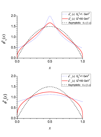
Figure 1: The $DA$ for the $q$ (upper panel) and $s$ (lower panel) flavor in the $\eta$ meson, at the initial scale $Q_{0}^{2}$ = 1 GeV² (dotted line) and after evolution to the scale $Q^{2}$ = 50 GeV² (full line). The asymptotic behavior is also shown for comparison (dashed line).

For $Q^{2}>Q_{0}^{2}$, the $\eta TFF$ is obtained through QCD evolution Efremov:1979qk ; Lepage:1979zb ; Mueller:1994cn . The $\eta DA$ can be expressed in terms of the Gegenbauer polynomials,

$$\phi_{\eta}^{q,s}(x,Q^{2})=6\,x\,(1-x)\sum_{n(even)=0}^{\infty}a_{n}^{q,s}\,C_{n}^{3/2}(2x-1)\left(\frac{\log\frac{Q^{2}}{\Lambda_{QCD}^{2}}}{\log\frac{Q_{0}^{2}}{\Lambda_{QCD}^{2}}}\right)^{-\gamma_{n}},$$ (26)

where $\gamma_{n}$ is the anomalous dimension

$$\gamma_{n}=\frac{C_{F}}{\beta}\left(1+4\sum_{k=2}^{n+1}\frac{1}{k}-\frac{2}{(n+1)(n+2)}\right),$$ (27)

$\beta=\frac{11N_{C}}{3}-\frac{2N_{f}}{3}$ is the beta function to lowest order and $C_{F}=\frac{N_{C}^{2}-1}{2N_{C}}.$ If the $a_{n}^{q,s}$ coefficients are known, using Eq. (26) in Eq. (20) and (19), the $\eta TFF$ is obtained for any $Q^{2}\gg\Lambda_{QCD}^{2}.$ Once $\phi_{\eta}^{q,s}\left(x,Q_{0}^{2}\right)$ are known at a given scale $Q_{0}^{2}$, the $a_{n}^{q,s}$ coefficients are obtained using the orthogonality property of the Gegenbauer polynomials

$$a_{n}^{q,s}=\frac{2}{3}\frac{2n+3}{\left(n+1\right)\left(n+2\right)}\int_{0}^{1}dx\,C_{n}^{3/2}(2x-1)\,\phi_{\eta}^{q,s}\left(x,Q_{0}^{2}\right)~{}.$$ (28)

In this scheme, the $\eta$ meson cannot couple to two gluons. This should not be a serious drawback of the approach, having the $\eta$ essentially an octet character under $SU(3)$ transformations.

We fix now the values of $Q_{0}$, $C_{3}$ and $M.$ The $Q_{0}$ scale is closely related to the choice of the $\Lambda_{QCD}$ value. We fix a scale of $Q_{0}=1$ GeV, together with $\Lambda_{QCD}=0.226\operatorname{GeV},$ in analogy with the previous analysis Noguera:2010fe . A natural condition to be satisfied is continuity between the low virtuality description of the $\eta TFF$ and the high virtuality description, provided by Eq (19). To minimize the model dependence, we use the parameterization of the CLEO collaboration Gronberg:1997fj for the description of the TFF in the LV region:

$$F_{\gamma\gamma^{\ast}\eta}^{LV}\left(Q^{2}\right)=\left[{\frac{64\pi\Gamma(\eta\rightarrow\gamma\gamma)}{(4\pi\alpha)^{2}m_{\eta}^{3}}}\right]{\frac{1}{1-{\frac{t}{\Lambda_{\eta}^{2}}}}}=\frac{F\left(0\right)}{1+\frac{Q^{2}}{\Lambda_{\eta}^{2}}}\,,$$ (29)

with $F\left(0\right)=0.272\pm 0.007\operatorname{GeV}^{-1},$ obtained using $\Gamma(\eta\rightarrow\gamma\gamma)=0.510\pm 0.026$ 10^-3 MeV as given by the Particle Data Group Nakamura:2010zzi together with $m_{\eta}=547.85$ MeV, and $\Lambda_{\eta}=774\pm 29$ MeV Gronberg:1997fj .

The value of the mass $M$ can be obtained equating the $\eta TFF$ given by Eq. (19) at $Q^{2}=Q_{0}^{2}$, using as $\Phi_{\eta}(x,Q_{0}^{2})$ the one provided by the NJL model, to the value given, at the same scale, by the monopole parametrization Eq. (19),

$$Q_{0}^{2}F_{\gamma\gamma^{\ast}\eta}^{LV}\left(Q_{0}^{2}\right)=\frac{Q_{0}^{2}F\left(0\right)}{1+\frac{Q_{0}^{2}}{\Lambda_{\eta}^{2}}}=\int_{0}^{1}\frac{dx}{x+\frac{M^{2}}{Q_{0}^{2}}}\Phi_{\eta}(x,Q_{0}^{2})+\frac{C_{3}}{Q_{0}^{2}}.$$ (30)

Finally, the only unknown is $C_{3}$, for which several reasonable values have been used, as discussed in the following section.

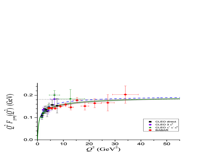
Figure 2: Calculation of the transition form factor via the $\eta DA$ with $M=0.557\operatorname{GeV}$, $\ C_{3}=2.04\,10^{-2}\operatorname{GeV}^{3}$ and using $Q_{0}^{2}=1\operatorname{GeV}^{2}$ (full-line) compared with the available experimental data :2011hk ; Gronberg:1997fj . The gray region describes the indeterminacy on $C_{3}$. The dashed line represents the result obtained taking $C_{3}=0$. The dotted line corresponds to the asymptotic value for the form factor.

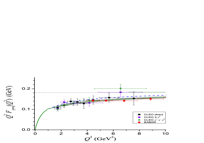
Figure 3: The same as in Fig 2, but in the low virtuality region

IV Results and discussion

	$\mu_{s}$	$m_{s}$	$\left\langle\bar{s}s\right\rangle^{1/3}$	$m_{K}$	$m_{\eta}$	$m_{\eta^{\prime}}$	$f_{K}/f_{\pi}$	$f_{\eta}^{q}/f_{\pi}$	$f_{\eta}^{s}/f_{\pi}$
Set I	171.2	430	$\ -186\$	497	541	1157	1.07	0.603	$\ -0.664$
Set II	184.2	435	$-184$	515	554	1148	1.07	0.832	$\ -0.840\$
Exp.			$-194$	495	548	958	1.18	0.828	$-0.848$

Table 1: We show results for two different parametrizations of the NJL model for several physical quantities, together with their experimental or phenomenological values. Explicit expressions for these are reported in the Appendix. The masses and the quark condensate are given in MeV.

We present now our results of the calculation of the $\eta TFF$. The starting point is the $\eta DA$, evaluated at the low energy scale of the model. According to Eq. (24), all we need is the value of the $\eta$ mass, the quark masses and the regularization parameter $\Lambda$. We use for the $\eta$ mass the experimental value, $m_{\eta}=548\operatorname{MeV}.$ The quark masses $m_{q(s)}$ and the regularization parameter $\Lambda$ have to be fixed within the NJL model. It is important to work in the Pauli-Villars regularization scheme, in order to preserve gauge invariance. Unfortunately, to our knowledge, all the available fits for the NJL model in $SU(3)$ are done within the cutoff regularization scheme. The only exception is the paper by Bernard and Vautherin Bernard:1988wi , where anyway an approximate expression for the $I_{2}(m_{i},m_{j,}q^{2})$ integral is used. Therefore, we have performed a new fit of the model parameters. The SU(3) NJL model gives a very good description for the meson properties Klimt:1989pm , but one has to be careful, since it does not include confinement. To avoid problems, we impose a value of $m_{u}>m_{\eta}/2.$ The details of the model (whose Lagrangian is given by Eq. (34)) are given in the Appendix. Here it is worth to recall only that the model has five parameters, which can be chosen as the current quark masses, $\mu_{u}$ and $\mu_{s}$, the dressed quark masses, $m_{u}$ and $m_{s},$ and the cutoff parameter, $\Lambda.$ Our strategy for the fits has been: i) the $m_{u}$ mass has been fixed to $275\operatorname{MeV};$ ii) $\mu_{u}$ and $\Lambda$ are determined by fitting $m_{\pi}$ and $f_{\pi};$ iii) $\mu_{s}$ and $m_{s}$ are chosen looking for an overall good description of the strange sector. In table 1 two different sets of the relevant quantities, obtained by the above described fitting procedure, are reported. It is seen that their experimental values are reproduced very well. In the Set I, we have imposed the additional condition for the resulting eta mass: $m_{\eta}\leq 2m_{u}.$ In this set, a very good description of masses in the strange sector is obtained, but paying the price of a worse description of $f_{\eta}^{\,q,s}.$ In Set II, the description of the masses is slightly worse, but the $f_{\eta}^{\,q,s}$ are very well reproduced. One should notice that, in going from $SU(2)$ to $SU(3)$ within the NJL model, the number of parameters moves from 3 to 5. One has therefore at hand two more parameters for explaining three new masses, three new decay constants and a new quark condensate. Actually, for calculating the $\eta DA$ only $m_{u}$ and $\Lambda$, which have the same value in both sets, are needed, together with $m_{s},$ which changes from 430 MeV in Set I to 435 MeV in Set II. With respect to these quantities, the predictions of the model are therefore reasonably stable. The results for the $\eta DA$ are presented for the following values of the parameters: $\Lambda=740\operatorname{MeV},$ $m_{u}=275\operatorname{MeV}$ and $m_{s}=435\operatorname{MeV}.$ It may be useful to reiterate that the obtained values of $f_{\eta}^{\,q,s}$ are not relevant for the present calculation, because we used the experimental ones.

In Fig. 1, the $\eta DA$ are shown. We observe that $\phi_{\eta}^{q}\left(x,Q_{0}^{2}\right)$ is peaked around the central point $x=0.5$ while $\phi_{\eta}^{s}\left(x\right)$ is relatively flat. This is a consequence of the masses of quarks $u$ and $d$, which are close to half the mass of the eta, while it is not the case for the mass of the strange quark. What is clearly seen is the following reasonable feature: the less bound is a system, the more narrow is its DA around the point $x=0.5$.

Our $DAs$ have an infinite expansion in terms of the Gegenbauer polynomials. The firsts coefficients $a_{\eta}^{q,s}$, defined in Eq. (28), at $Q_{0}^{2}=1\operatorname{GeV}^{2}$ are:

$$a_{2}^{q} =0.134\ \ \ \ \ \ \ \ \ \ \ \ \ \ a_{2}^{s}=0.377$$

$$a_{4}^{q} =0.352\ \ \ \ \ \ \ \ \ \ \ \ \ \ a_{4}^{s}=0.245$$ (31)

The $a_{\eta}^{s}$ coefficients are close to the values predicted by a flat distribution. On the other hand side, we observe that $a_{2}^{q}<a_{4}^{q},$ at variance with what is commonly used in the field. This feature is due to the narrow structure of $\phi_{\eta}^{q}\left(x\right).$ We can compare our results with the values used by other authors. The $a_{2}^{q}$ and $a_{2}^{s}$ coefficients are to be compared to the parameter $B=0.3$ used in Ref. Wu:2011gf .

In Ref. Kroll:2010bf the values $a_{2}^{1}=-0.06\pm 0.06,$ $a_{2}^{8}=-0.07\pm 0.04$ and ${a}_{2}^{\pi}{=0.22\pm 0.06}$ are given, but at $Q^{2}=4\operatorname{GeV}^{2}.$ From Eq. (31) and using $\phi_{\eta}^{1}=(5\,\phi_{\eta}^{q}+\phi_{\eta}^{s})/6$ and $\phi_{\eta}^{8}=(5\,\phi_{\eta}^{q}-2\,\phi_{\eta}^{s})/3$ we obtain

$$a_{2}^{1}\left(1\operatorname{GeV}^{2}\right)=0.17\ \ \ \ \ \ \ \ \ \ \ a_{2}^{8}\left(1\operatorname{GeV}^{2}\right)=-0.028\ \ .$$ (32)

Evolving these results we have

$$a_{2}^{1}\left(4\operatorname{GeV}^{2}\right)=0.14\ \ \ \ \ \ \ \ \ \ \ a_{2}^{8}\left(4\operatorname{GeV}^{2}\right)=-0.022~{}~{}.$$ (33)

The value for $a_{2}^{8}$ is therefore consistent with that used in Ref. Kroll:2010bf , while some difference is found for the value of $a_{2}^{1}$. In the pion case, if we use a flat distribution at $Q_{0}^{2}=1\operatorname{GeV}^{2},$ a value $a_{2}^{\pi}\left(4\operatorname{GeV}^{2}\right)=0.31$ is obtained. In Ref. Brodsky:2011yv it has been noted that the values for these parameters found in Kroll:2010bf suggest a very large SU(3) breaking between the $DA$ of the $\pi^{0}$ and the one of $\eta^{8},$ and a very little U(1) symmetry breaking between $\eta^{8}$ and $\eta^{1}.$ Our results show the same structure of those of Ref Kroll:2010bf , at least for $a_{2}^{8}$ and for the big difference between $a_{2}^{\pi}$ and $a_{2}^{8}.$ The origin of this difference is in the small value of $a_{2}^{q}$ due to the narrow structure of $\phi_{\eta}^{q}(x)$, originated by the fact that $m_{u}$ is close to $m_{\eta}/2.$ At the same time, a small value of $a_{2}^{q}$ explains a small value for $a_{2}^{1}.$ One should remember that the present scheme reproduces the SU(3)_F and U(3)_F symmetry breaking in the pseudoscalar meson sector.

The results of Eq. (32) are also in good agreement with those from Agaev:2010zz ; Agaev:2003kb . In the latter references, the authors give their results for $Q_{0}^{2}=1\operatorname{GeV}^{2}$ in terms of the quantities $B_{2}^{q}$ and $B_{2}^{g},$defined in Agaev:2003kb and related to our expressions as follows : $a_{2}^{1}\left(1\operatorname{GeV}^{2}\right)=-B_{2}^{q}+B_{2}^{g}/102$ and $a_{2}^{8}\left(1\operatorname{GeV}^{2}\right)=-B_{2}^{q}.$ Using the numerical results of Ref Agaev:2010zz , we have $a_{2}^{1}\left(1\operatorname{GeV}^{2}\right)=0.149\pm 0.048$ and $a_{2}^{8}\left(1\operatorname{GeV}^{2}\right)=-0.0425\pm 0.0175,$ to be compared to our results, Eq. (32). In these papers, the coupling of a two gluon state to the singlet $\bar{q}q$ component of the $\eta$ mesons is introduced explicitely, providing a contribution, $B_{2}^{g}$, which is an important part of the final result. In absence of gluons, the symmetry $U(1)$ is not broken. In our case, the $U(1)$ symmetry is broken through the ’t Hooft interaction term 'tHooft:1986nc  introduced in the Lagrangian (34), making our results consistent with those of refs. Agaev:2010zz ; Agaev:2003kb .

As stated at the end of the previous section, once the $\eta DA$ has been obtained at the scale $Q_{0}^{2}$ and evolved to $Q^{2}$ according to Eqs. (26)-(28), the only remaining unknown for the evaluation of the $\eta TFF$ according to Eq. (19) is the constant $C_{3}$ of the higher twist term. To this aim, three different scenarios have been considered, corresponding to a contribution from this term to the form factor at $Q_{0}^{2}=1\operatorname{GeV}^{2}$ of 10% $(C_{3}=1.02\cdot 10^{-2}\operatorname{GeV}^{3})$, 20% $(C_{3}=2.04\cdot 10^{-2}\operatorname{GeV}^{3})$ and 30% $(C_{3}=3.06\cdot 10^{-2}\operatorname{GeV}^{3})$. The cutoff parameter $M$ varies between 487 MeV, for $C_{3}=1.02\cdot 10^{-2}\operatorname{GeV}^{3},$ 557 Mev, for $C_{3}=2.04\cdot 10^{-2}\operatorname{GeV}^{3},$ and 638 MeV, $C_{3}=3.06\cdot 10^{-2}\operatorname{GeV}^{3}.$ We show in Fig 2 the obtained result for $\eta TFF$ and in Fig. 3 a detail of the region between $Q^{2}=0$ and $Q^{2}=10\operatorname{GeV}^{2}.$

The results for the $\eta TFF$, shown in Figs. 2 and 3, exhibit a very good description of the experimental data in the whole kinematic region. For completeness we have included in the figures the $C_{3}=0$ case and the asymptotic vale for the $\eta TFF,$ $Q^{2}F_{\gamma\gamma^{\ast}\eta}\left(Q^{2}\right)=(5\sqrt{2}f_{\eta}^{\,q}+2f_{\eta}^{\,s})=0.181\operatorname{GeV}.$ It may be interesting to notice that the value of the asymptotic $\eta TFF$ is very close to the value of the asymptotic $\pi TFF,$ $Q^{2}F_{\gamma\gamma^{\ast}\pi}\left(Q^{2}\right)=\sqrt{2}f_{\pi}=0.185\operatorname{GeV}.$ It is also clear that, at variance with what happens in the $\pi$ case, to explain the eta data some $C_{3}$ contribution may be needed only in the region around $Q^{2}=20-30\operatorname{GeV}^{2}$. Anyway, a complete discussion is obtained only by comparing the present results for the $\pi TFF$ with those of Ref. Noguera:2010fe . In the $\pi$ case, the $\ C_{3}$ contribution was crucial to reproduce the data in the region $Q^{2}=10-20\operatorname{GeV}^{2}$ and the calculated $\pi TFF$ crossed the asymptotic curve quite early (around $Q^{2}=10\operatorname{GeV}^{2})$ and with a significative slope. In the $\eta$ case, the situation is less dramatic: the higher twist term improves the TFF description only slowly, and the theoretical result crosses softly the asymptotic value around $Q^{2}=40\operatorname{GeV}^{2}.$

Another interesting point is the stability of the parameters. In calculating the $\eta TFF$, we have adopted a procedure independent from that used in Ref. Noguera:2010fe , namely, $C_{3}$ and $M$ have been fitted using the $\eta$ data only. The parameters used in both calculations have been $\Lambda_{QCD}=0.226\operatorname{GeV}$ and $Q_{0}=1\operatorname{GeV}.$ Otherwise, in Ref Noguera:2010fe , a fully model independent calculation was performed, choosing $\phi_{\pi}\left(x\right)=1$ on the basis of chiral symmetry. Here one is forced to choose a model for the description of the $\eta DA$ at $Q_{0}^{2},$ and $C_{3}$ and $M$ have been fixed within this model, independently from the $\pi$ case. Despite of this, the result obtained in the two calculations are quite consistent. Varying the weight of the higher twist term from 10% to 30% produces a change in $C_{3}$ from $1.02\cdot 10^{-2}\operatorname{GeV}^{3}$ to $3.06\cdot 10^{-2}\operatorname{GeV}^{3}$ in the $\eta$ case, to be compared to a variation of $C_{3}$ from $0.99\cdot 10^{-2}\operatorname{GeV}^{3}$ to $2.98\cdot 10^{-2}\operatorname{GeV}^{3}$ in the $\pi$ case. The agreement is impressive.

On the other hand side, we found for the mass parameter a wider variation. In the $\eta$ case one gets $M=560\pm 70\operatorname{MeV}$,taking into account the uncertainty in $C_{3},$ to be compared to $M=620\pm 70\operatorname{MeV}$ for the $\pi$ case. Despite of these differences, the results can be considered perfectly consistent with each other. The difference in the central value of $M$ could imply that, for the pion, a larger contribution from the transverse momentum is expected with respect to that for the eta particle. It is indeed what has been obtained in Refs. Kroll:2010bf ; Wu:2011gf . The values of $M$ could be compared with the value of $\left\langle k_{\perp}\right\rangle$ given by P. Kroll Kroll:2010bf , $\left\langle k_{\perp}\right\rangle\simeq 710\operatorname{MeV}$ for the pion and $\left\langle k_{\perp}\right\rangle\simeq 390-440\operatorname{MeV}$ for the eta. It can be also compared with the $\beta_{\pi}$ parameter used by Wu:2011gf , which is related with the width of the gaussian distribution of transverse momentum used by these authors, with the values $\beta_{\pi}=668\operatorname{MeV}$ for the $u$-quark and $\beta_{\pi}\simeq 530\operatorname{MeV}$ for the $s$-quark. A comparison of our parameters, based on a quark-flavor decomposition of the relevant quantities (DAs, decay constants), with those used in Ref. Xiao:2005af , obtained within a singlet-octet decomposition, is instead rather involved. The spirit of the present calculation and those of Refs. Xiao:2005af ; Wu:2011gf are rather different. In our calculation, the known QCD evolution of the $DA$ governs the $Q^{2}$ dependence of the form factor. The same $Q^{2}$ dependence is obtained, in Refs. Xiao:2005af ; Wu:2011gf , through the $k_{T}$ dependence assumed for the light-cone wave function of the mesons. It is therefore significant that the two approaches provide similar results, describing probably, using different tools, a similar mechanism.

In the present discussion, the result on $\gamma^{\ast}\left(q\right)\rightarrow P\gamma,$ reported by BaBar for a time like $q^{2}=112\operatorname{GeV}^{2},$ ${q}^{2}{F}_{\gamma\gamma^{\ast}\eta}\left(q^{2}\right){=0.229\pm 0.030\pm 0.008\operatorname{GeV}}$, has not been included. The reason is that the kinematics and dynamics of this process is different from the ones studied here. There is no symmetry relating $F_{\gamma\gamma^{\ast}P}(q^{2})$ at one point $q^{2}$ to $F_{\gamma\gamma^{\ast}P}(Q^{2})$ in the point $Q^{2}=-q^{2}$. The coincidence is in the asymptotic value, which has been predicted for this process to beLepage:1980fj $-q^{2}F_{\gamma\gamma^{\ast}P}\left(q^{2}\right)=\sqrt{2}f_{P}\,(1-5\,\alpha_{s}\left(q^{2}\right)/3\pi),$ when the contribution coming from the $\alpha_{s}\left(q^{2}\right)$ term could be disregarded. In the present scheme we obtain $Q^{2}F_{\gamma\gamma^{\ast}P}(Q^{2})=0.19$ GeV at $Q^{2}=112$ GeV${}^{2},$ which implies a very slowly growing behavior of the $TFF$ even for these high values of the virtuality.

In closing this section, it is useful to list items that prevent from using the same formalism for the description of the $\eta^{\prime}TFF$. First of all, as it has been previously noted, the NJL does not include confinement. Therefore, if one uses the same expression, Eq. (24), in the $\eta^{\prime}$ case, an imaginary part will appear in the DA at some value of $x$. Secondly, the $\eta^{\prime}$ is basically a singlet state and it can mix strongly with the two gluons state or, later, with some $c\bar{c}$ component. These ingredients are not included in the present formalism.

V Conclusions

In this paper, the $\eta TFF$ has been discussed in a formalism which connects a low energy description of the hadron involved with a high energy description based on a QCD perturbative formulation. The two descriptions are matched at some scale $Q_{0}^{2}$. The scheme has been applied to describe the parton and generalized parton distributions with notable successTraini:1997jz ; Scopetta:1997wk ; Scopetta:1998sg ; Theussl:2002xp ; Courtoy:2008nf and, in particular, to the $\pi TFF$ in Noguera:2010fe . The formalism selects therefore two regions of virtuality, separated at $Q_{0}^{2}.$ For $Q^{2}<Q_{0}^{2}$, use has been made of the experimental parametrization of the $\eta TFF$ data. This has been done to avoid model dependence in this region. At $Q^{2}>Q_{0}^{2}$, use has been made of a high virtuality description, which incorporates the following important physical ingredients: i) a $\eta DA$ obtained in the NJL model ; ii) a mass cut-off in the definition of the $\eta TFF$ from the $\eta DA,$ $M,$ Radyushkin:2009zg which, interpreted from the point of view of constituent models, takes into account the constituent mass, transverse momentum effects and also higher twist effects; iii) an additional higher twist term into the definition of the $\eta TFF$ in the high virtuality description, parameterized by a unique constant, $C_{3}$; iv) the two descriptions have to match at a virtuality $Q_{0}^{2}$, a scale which is universal and should be the same for all observables.

In section II it has been shown that the dominant, twist two, expression for the pseudoscalar $TFF,$ given in Eq. (14) has to be corrected, for including higher twist effects. The minimal correction would be the one given in Eq. (19).

The $\eta DA$ at $Q_{0}^{2}$ has been obtained in the NJL model. For that, the parameters have been adjusted for a good reproduction of the $\eta$ sector with the Pauli-Villars regularization. The obtained fits represent an overall good description of the strange sector, not only for the masses, but also for the meson decay constants. It is worth to strees that, in going from SU(2) to SU(3), the number of parameters is increased by two, while the number of new physical quantities, included in Table 1, are seven. The obtained DAs in this model show consystency with other analyses,where the DAs are parametrized Kroll:2010bf ; Agaev:2010zz ; Wu:2011gf .

Using $Q_{0}=1\operatorname{GeV}$ as matching point, the higher virtuality results of the $\eta TFF$ are well reproduced. The $C_{3}$ term turns out to be relatively small. Its effect is to reduce the value of the contribution to the twist two $\eta TFF$ only for $Q^{2}<5$ GeV². Its value, $C_{3}=2.04\cdot 10^{-2}\operatorname{GeV}^{3}$ for a 20% of higher twist contamination at $Q_{0}^{2},$ is in perfect agreement with the one obtained for the $\pi TFF$ in Ref. Noguera:2010fe , $C_{3}=1.98\cdot 10^{-2}\operatorname{GeV}^{3}.$ Moreover, the results are very stable with respect to variations of this parameter.

The value obtained for $M=560\operatorname{MeV}$ is comparable with that of the pion case in Ref Noguera:2010fe , $M=620\operatorname{MeV}.$ The relative high value of $M$ in both cases can be understood thinking that it includes the constituent quark mass, the mean value of the transverse quark momentum and other higher twist contributions. In turn, the higher value of $M$ for the $\pi$ than for the $\eta$ can be related to the fact that the contribution of the quark transverse momentum in the $\pi$ case is expected to be more important with respect to the $\eta$ case Kroll:2010bf ; Wu:2011gf .

The calculation proves that all the BaBar results can be accommodated in the present scheme, which only uses standard QCD ingredients and low virtuality data. It must be emphasized that, in order to have a good description for both $\pi$ and $\eta$, higher twist effects are important, as the modification from Eq. (14) to Eq. (19) signals. It must be also noted that the matching scale is as high as $1$ GeV, a feature already found in the description of parton distributions when precision was to be attained. With these ingredients, the calculation shows an excellent agreement with the data.

Let us conclude by stressing that we have justified the formalism developed in Ref. Noguera:2010fe  to describe the $\pi TFF$ and we have extended it to the $\eta TFF.$ The idea of the approach is that one can use models or effective theories to describe the non perturbative sector, and QCD to describe the perturbative one. In here, we have preferred to use data for the low virtuality sector to avoid model dependence, but in building the $\eta DA$ at $Q_{0}^{2}$ we have used the NJL model. Higher twist effects (parametrized in our case by $M$ and $C_{3}$) are small but crucial in order to attain an excellent description of the $\pi$ and $\eta$ experimental results.

Appendix A The $SU(3)$ NJL model for pseudoscalars mesons.

In calculating the $\eta DA$, the minimal extension of the NJL model for describing pseudoscalar mesons in SU(3), proposed in Ref Bernard:1987sg , has been used:

$$\mathcal{L} =\bar{q}\left(x\right)\left(i\hbox to0.0pt{$/$\hss}\partial-\mu\right)q\left(x\right)+G\sum_{a=0}^{8}\left[\left(\bar{q}\lambda^{a}q\right)^{2}+\left(\bar{q}i\gamma_{5}\lambda^{a}q\right)^{2}\right]-$$

$$-K\,\left[\det\left(\bar{q}\left(1+\gamma_{5}\right)q\right)+\det\left(\bar{q}\left(1-\gamma_{5}\right)q\right)\right]\quad,$$ (34)

where $\mu=\mathrm{diag}[\mu_{u},\mu_{d},\mu_{s}]$ is the matrix of the current quark masses and $\lambda^{a},$ $a=0,...,8,$ are the SU(3) generators. SU(2) will be considered a good symmetry, and, therefore, $\mu_{u}=\mu_{d}.$ As it is well known, the first consequence of the scalar interaction term is to provide the constituent quark masses, $m_{u}=m_{d},\ m_{s},$ different from the current ones. The main results are summarized here, while the reader is referred to the section IV-B of Ref. Klevansky:1992qe for details.

By defining the integrals:

$$I_{1}\left(m\right) =i\int\frac{d^{4}p}{\left(2\pi\right)^{4}}\frac{1}{\left(p^{2}-m^{2}+i\epsilon\right)}~{},$$

$$I_{2}\left(m_{i},m_{j},q^{2}\right) =i\int\frac{d^{4}p}{\left(2\pi\right)^{4}}\frac{1}{\left(p^{2}-m_{i}^{2}+i\epsilon\right)\left[\left(p-q\right)^{2}-m_{j}^{2}+i\epsilon\right]}~{},$$ (35)

the constituent masses are given by

$$m_{u} =\mu_{u}+16\,G\,N_{c}\,m_{u}\,I_{1}\left(m_{u}\right)+32\,K\,N_{c}^{2}\,m_{u}\,I_{1}\left(m_{u}\right)\,m_{s}\,I_{1}\left(m_{s}\right)~{},$$

$$m_{s} =\mu_{s}+16\,G\,N_{c}\,m_{s}\,I_{1}\left(m_{s}\right)+32\,K\,N_{c}^{2}\,\left[m_{u}\,I_{1}\left(m_{u}\right)\right]^{2}~{},$$ (36)

where $N_{c}$ is the number of colors. The vacuum expectation values for the condesates of the quarks of flavor $q_{i}$ are

$$\left\langle\bar{q}_{i}q_{i}\right\rangle=4\,m_{i}\,I_{1}\left(m_{i}\right)-4\,\mu_{i}\,I_{1}\left(\mu_{i}\right)~{},$$ (37)

where the expectation value of the $\bar{q}q$ in the perturbative vacuum has been substracted from the expectation value in the true vacuum. The last term in Eq. (37) is negligible in the $u-d$ quark sector, while it becomes important in the strange sector.

The next step is the description of the pseudoscalar states. For the pion and kaon case, by defining the quantities

$$K_{3} =G+2\,N_{c}\,K\,m_{s}\,I_{1}\left(m_{s}\right)~{},$$

$$K_{6} =G+2\,N_{c}\,K\,m_{u}\,I_{1}\left(m_{u}\right)~{},$$ (38)

and

$$D\left(m_{i},m_{j},q^{2}\right)=I_{1}\left(m_{i}\right)+I_{1}\left(m_{j}\right)+\left(\left(m_{i}-m_{j}\right)^{2}-q^{2}\right)\,I_{2}\left(m_{i},m_{j},q^{2}\right)~{},$$ (39)

one has that the pion and kaon masses are obtained solving the equations:

$$1-8\,N_{c}\,K_{3}\,D\left(m_{u},m_{u},m_{\pi}^{2}\right) =0~{},$$

$$1-8\,N_{c}\,K_{6}\,D\left(m_{u},m_{s},m_{K}^{2}\right) =0~{}.$$ (40)

The couplings of the pion and the kaon to the quarks are given by:

$$g_{\pi qq}^{2}=\left[4\,N_{c}\,\frac{d}{dq^{2}}D\left(m_{u},m_{u},q^{2}\right)\right]_{q^{2}=m_{\pi}^{2}}^{-1}~{},$$

$$g_{Kqq}^{2}=\left[4\,N_{c}\,\frac{d}{dq^{2}}D\left(m_{u},m_{s},q^{2}\right)\right]_{q^{2}=m_{K}^{2}}^{-1}~{},$$ (41)

and the decay constants are:

$$F_{\pi}=-4\,N_{c}\,g_{\pi qq}\,m_{u}\,I_{2}\left(m_{u},m_{u},m_{\pi}^{2}\right)~{},$$ (42)

$$F_{K}=\frac{2\,N_{c}\,g_{Kqq}}{m_{K}^{2}}\,\left\{\left(m_{s}+m_{u}\right)\,D\left(m_{u},m_{s},m_{K}^{2}\right)-2\,m_{u}\,I_{1}\left(m_{u}\right)-2\,m_{s}\,I_{1}\left(m_{s}\right)\right\}~{},$$ (43)

where $F_{\pi,K}=f_{\pi,K}/\sqrt{2}$.

The $\eta$ particle deserves a more careful discussion, due to its mixing with the $\eta^{\prime}$ particle. Working in the flavor basis, one can define

$$K_{q} =G-2\,N_{c}\,K\,m_{s}\,I_{1}\left(m_{s}\right)~{},$$

$$K_{qs} =-2\sqrt{2}\,N_{c}\,K\,m_{u}\,I_{1}\left(m_{u}\right)~{},$$ (44)

$${\mathcal{K}} =K_{q}\,G-K_{qs}^{2}~{}.$$

The interaction in the $\eta-\eta^{\prime}$ sector can be described by the expression

$$\left(i\gamma_{5}\lambda^{i}\right)\left[M_{ij}\right]\left(i\gamma_{5}\lambda^{j}\right)$$ (45)

with $i,j=q,s$, $\lambda^{q}=\mathrm{diag}[1,1,0]$, $\lambda^{s}=\mathrm{diag}[0,0,\sqrt{2}]$ and the interaction matrix is given by

$$\left[M_{ij}\right]=\frac{1}{D_{\eta}}\left(\begin{array}[c]{cc}a_{qq}&a_{qs}\\ a_{qs}&a_{ss}\end{array}\right)~{},$$ (46)

with

$$a_{qq} =2\left(K_{q}-8\,{\mathcal{K}}\,N_{c}\,D\left(m_{s},m_{s},q^{2}\right)\right)~{},$$

$$a_{ss} =2\left(G-8\,{\mathcal{K}}\,N_{c}\,D\left(m_{u},m_{u},q^{2}\right)\right)~{},$$

$$a_{qs} =2\,K_{qs}~{},$$ (47)

$$D_{\eta}\left(q^{2}\right) =(a_{qq}a_{ss}-a_{qs}^{2})/(4{\mathcal{K}})~{}.$$

The $\eta$ mass is obtained solving the equation

$$D_{\eta}\left(m_{\eta}^{2}\right)=0~{}.$$ (48)

In a neighborhood of $q^{2}=m_{\eta}^{2}$ the interaction can be written as

$$\left(-\sin\phi\,\lambda^{s}+\cos\phi\,\lambda^{q}\right)\frac{-g_{\eta qq}}{q^{2}-m_{\eta}^{2}}\left(-\sin\phi\,\lambda^{s}+\cos\phi\,\lambda^{q}\right)$$

$$=\frac{a_{qq}}{D_{\eta}}\left(\epsilon_{\eta}\,\lambda^{s}+\lambda^{q}\right)\left(\epsilon_{\eta}\,\lambda^{s}+\lambda^{q}\right)~{},$$ (49)

with $\epsilon_{\eta}=a_{qs}/a_{qq}.$ In obtaining the right hand side of this equation, use has been made of Eq. (48), which implies $a_{ss}=a_{qs}^{2}/a_{qq}.$ From (49) one has

$$\cos\phi=\frac{1}{\sqrt{1+\epsilon_{\eta}^{2}}}\ \ ,\ \ \ \ \ \ \ \ \ \ \ \sin\phi=\frac{-\epsilon_{\eta}}{\sqrt{1+\epsilon_{\eta}^{2}}}~{},$$

$$g_{\eta qq}^{2}=-\left.\frac{\left(1+\epsilon_{\eta}^{2}\right)\,a_{qq}}{dD_{\eta}/dq^{2}}\right|_{q^{2}=m_{\eta}^{2}}~{}.$$ (50)

For the flavor decay constants, one has

$$F_{\eta}^{q} =-12\,g_{\eta qq}\,\cos\phi\,m_{u}\,I_{2}\left(m_{u},m_{u},m_{\eta}^{2}\right)~{},$$

$$F_{\eta}^{s} =12\,g_{\eta qq}\,\sin\phi\,m_{s}\,I_{2}\left(m_{s},m_{s},m_{\eta}^{2}\right)~{},$$ (51)

where $F_{\eta}^{q,s}=f_{\eta}^{q,s}/\sqrt{2}$.

We need to evaluate the integrals defined in Eq. (35). Due to the point-like character of the interaction, the lagrangian Eq. (34) is not renormalizable and a regularization procedure for these integrals has to be defined. We use the Pauli-Villars regularization in order to render the occurring integrals finite. This means that, for integrals like the ones defined in Eq. (35), we make the following replacement,

$$I_{1}\left(m_{i}\right)\longrightarrow\sum_{\ell=0}^{2}c_{\ell}\,I_{1}\left(M_{\ell,i}\right)\ \ \ \ \ \ \ \ I_{2}\left(m_{i},m_{j},q^{2}\right)\longrightarrow\sum_{\ell=0}^{2}c_{\ell}\,I_{2}\left(M_{\ell,i},M_{\ell,j},q^{2}\right)$$ (52)

with $M_{\ell,j}^{2}=m_{j}^{2}+\ell\,\Lambda^{2}$, $c_{0}=c_{2}=1,$ $c_{1}=-2.$ Here, for simplicity, we choose the same $\Lambda$ value for the strange and the nonstrange sector. According to these prescriptions one finds

$$I_{1}\left(m_{i}\right)=\frac{1}{16\,\pi^{2}}\left[-2\,M_{1,i}^{2}\ln\frac{M_{1,i}^{2}}{m_{i}^{2}}+M_{2,i}^{2}\ln\frac{M_{2,i}^{2}}{m_{i}^{2}}\right]~{},$$ (53)

$$I_{2}\left(m_{i},m_{j},q^{2}\right)=\frac{1}{32\pi^{2}}\sum_{\ell=0}^{2}c_{\ell}\left[\left(\ln\frac{M_{1,i}^{2}}{m_{i}^{2}}+\ln\frac{M_{1,j}^{2}}{m_{j}^{2}}\right)+\frac{M_{1,j}^{2}-M_{1,i}^{2}}{q^{2}}\ln\frac{M_{\ell,j}^{2}}{M_{\ell,i}^{2}}+\Phi_{\ell}\right]~{},$$ (54)

with

$$\Phi_{\ell}=\frac{2}{q^{2}}\sqrt{-\lambda\left(M_{\ell,i}^{2},M_{\ell,j}^{2},q^{2}\right)}\left[\arctan\frac{q^{2}+M_{1,j}^{2}-M_{1,i}^{2}}{\sqrt{-\lambda\left(M_{\ell,i}^{2},M_{\ell,j}^{2},q^{2}\right)}}+\arctan\frac{q^{2}-M_{1,j}^{2}+M_{1,i}^{2}}{\sqrt{-\lambda\left(M_{\ell,i}^{2},M_{\ell,j}^{2},q^{2}\right)}}\right]$$ (55)

where $\lambda\left(M_{\ell,i}^{2},M_{\ell,j}^{2},q^{2}\right)$ is the Källén lambda.

Now, we fix the parameters of the model. Looking at the lagrangian, we have a five parameters model, $\mu_{u},$ $\mu_{s},$ $G,$ $K$ and $\Lambda.$ Nevertheless, it is more intuitive to organize the fit of the parameters in terms of $\mu_{u},$ $\mu_{s},$ $m_{u},$ $m_{s}$ and $\Lambda,$ using equations (36) to determine $G$ and $K.$ We impose $m_{u}=275\operatorname{MeV},$ in order to have $m_{\eta}^{\exp}<2m_{u}.$ Then, $\mu_{u}$ and $\Lambda$ are obtained in recovering the values of $F_{\pi}$ and $m_{\pi}.$ At this step one has

$$\mu_{u}=6.69\operatorname{MeV},\ \ m_{u}=275\operatorname{MeV},\ \ \Lambda=740\operatorname{MeV}\ \ \longrightarrow\ \ \ m_{\pi}=138\operatorname{MeV},\ \ F_{\pi}=92.2\operatorname{MeV},\ \ \left\langle\bar{u}u\right\rangle=\left(-227\operatorname{MeV}\right)^{3}$$

determining the SU(2) sector. Then, $\mu_{s}$ and $m_{s}$ have been fixed by requiring a good overall fit of masses ($m_{K},$ $m_{\eta},$ $m_{\eta^{\prime}})$ and decay constants ($F_{K},$ $F_{\eta}^{q},$ $F_{\eta}^{s}).$ In table 1 two different sets of parameters are given, together with the obtained results. Using set I, by imposing $m_{\eta}\leq 2m_{u},$ a good agreement for the masses and a slightly less good agreement for the $F_{\eta}^{q,s}$ is obtained. On the other hand, in set II a very good agreement for $F_{\eta}^{q,s}$ is obtained, with a slightly worse result for the masses.

In the light-front calculation one needs the integral

$$\tilde{I}_{2}\left(x,m_{i},m_{P}^{2}\right) =i\int\frac{d^{4}k}{(2\pi)^{4}}\,\,\frac{\delta\left(x-1+\frac{k^{+}}{P^{+}}\right)}{\left[(k-P)^{2}-m_{i}^{2}+i\epsilon\right]\left(k^{2}-m_{i}^{2}+i\epsilon\right)}$$

$$=-\theta(x)\theta(1-x)\,\frac{1}{(4\pi)^{2}}\,\sum_{\ell=1}^{2}c_{\ell}\,\ln\,\frac{m_{i}^{2}-(1-x)\,x\,m_{P}^{2}}{M_{\ell,i}^{2}-(1-x)\,x\,m_{P}^{2}}\qquad.$$ (56)

Clearly, all one needs to calculate the $\eta DA$ are the $\eta$ and quark masses and the value of the cutoff parameter. For the DA calculations, the values $m_{u}=275\operatorname{MeV},$ $m_{s}=435\operatorname{MeV},$ $\Lambda=740\operatorname{MeV}$ and $m_{\eta}=548\operatorname{MeV}$ have been chosen.

References

(1)B. Aubert et al. [The BABAR Collaboration],
Phys. Rev. D 80 (2009) 052002 [arXiv:0905.4778 [hep-ex]].
(2)P. del Amo Sanchez et al. [ BABAR Collaboration ],
Phys. Rev. D84 (2011) 052001. [arXiv:1101.1142 [hep-ex]].
(3)A. V. Radyushkin,
Phys. Rev. D 80 (2009) 094009 [arXiv:0906.0323 [hep-ph]].
(4)M. V. Polyakov,
JETP Lett. 90 (2009) 228 [arXiv:0906.0538 [hep-ph]].
(5)S. V. Mikhailov and N. G. Stefanis,
Mod. Phys. Lett. A 24 (2009) 2858 [arXiv:0910.3498 [hep-ph]].
(6)A. E. Dorokhov,
Nucl. Phys. Proc. Suppl. 198 (2010) 190-193. [arXiv:0909.5111 [hep-ph]].
(7)N. I. Kochelev, V. Vento,
Phys. Rev. D81, 034009 (2010). [arXiv:0912.2172 [hep-ph]].
(8)S. Noguera and V. Vento,
Eur. Phys. J. A 46, 197 (2010) [arXiv:1001.3075 [hep-ph]].
(9)E. R. Arriola, W. Broniowski,
Phys. Rev. D81, 094021 (2010). [arXiv:1004.0837 [hep-ph]].