Adaptive Hedge

Abstract

Most methods for decision-theoretic online learning are based on the Hedge algorithm, which takes a parameter called the learning rate. In most previous analyses the learning rate was carefully tuned to obtain optimal worst-case performance, leading to suboptimal performance on easy instances, for example when there exists an action that is significantly better than all others. We propose a new way of setting the learning rate, which adapts to the difficulty of the learning problem: in the worst case our procedure still guarantees optimal performance, but on easy instances it achieves much smaller regret. In particular, our adaptive method achieves constant regret in a probabilistic setting, when there exists an action that on average obtains strictly smaller loss than all other actions. We also provide a simulation study comparing our approach to existing methods.

1 Introduction

Decision-theoretic online learning (DTOL) is a framework to capture learning problems that proceed in rounds. It was introduced by Freund and Schapire [1] and is closely related to the paradigm of prediction with expert advice [2, 3, 4]. In DTOL an agent is given access to a fixed set of $K$ actions, and at the start of each round must make a decision by assigning a probability to every action. Then all actions incur a loss from the range $[0,1]$, and the agent’s loss is the expected loss of the actions under the probability distribution it produced. Losses add up over rounds and the goal for the agent is to minimize its regret after $T$ rounds, which is the difference in accumulated loss between the agent and the action that has accumulated the least amount of loss.

The most commonly studied strategy for the agent is called the Hedge algorithm [1, 5]. Its performance crucially depends on a parameter $\eta$ called the learning rate. Different ways of tuning the learning rate have been proposed, which all aim to minimize the regret for the worst possible sequence of losses the actions might incur. If $T$ is known to the agent, then the learning rate may be tuned to achieve worst-case regret bounded by $\sqrt{T\ln(K)/2}$, which is known to be optimal as $T$ and $K$ become large [4]. Nevertheless, by slightly relaxing the problem, one can obtain better guarantees. Suppose for example that the cumulative loss $L^{*}_{T}$ of the best action is known to the agent beforehand. Then, if the learning rate is set appropriately, the regret is bounded by $\sqrt{2L^{*}_{T}\ln(K)}+\ln(K)$ [4], which has the same asymptotics as the previous bound in the worst case (because $L^{*}_{T}\leq T$) but may be much better when $L^{*}_{T}$ turns out to be small. Similarly, Hazan and Kale [6] obtain a bound of $8\sqrt{\text{VAR}_{T}^{\text{max}}\ln(K)}+10\ln(K)$ for a modification of Hedge if the cumulative empirical variance $\text{VAR}_{T}^{\text{max}}$ of the best expert is known. In applications it may be unrealistic to assume that $T$ or (especially) $L^{*}_{T}$ or $\text{VAR}_{T}^{\text{max}}$ is known beforehand, but at the cost of slightly worse constants such problems may be circumvented using either the doubling trick (setting a budget on the unknown quantity and restarting the algorithm with a double budget when the budget is depleted) [4, 7, 6], or a variable learning rate that is adjusted each round [4, 8].

Bounding the regret in terms of $L^{*}_{T}$ or $\text{VAR}_{T}^{\text{max}}$ is based on the idea that worst-case performance is not the only property of interest: such bounds give essentially the same guarantee in the worst case, but a much better guarantee in a plausible favourable case (when $L^{*}_{T}$ or $\text{VAR}_{T}^{\text{max}}$ is small). In this paper, we pursue the same goal for a different favourable case. To illustrate our approach, consider the following simplistic example with two actions: let $0<a<b<1$ be such that $b-a>2\epsilon$. Then in odd rounds the first action gets loss $a+\epsilon$ and the second action gets loss $b-\epsilon$; in even rounds the actions get losses $a-\epsilon$ and $b+\epsilon$, respectively. Informally, this seems like a very easy instance of DTOL, because the cumulative losses of the actions diverge and it is easy to see from the losses which action is the best one. In fact, the Follow-the-Leader strategy, which puts all probability mass on the action with smallest cumulative loss, gives a regret of at most $1$ in this case — the worst-case bound $O(\sqrt{L^{*}_{T}\ln(K)})$ is very loose by comparison, and so is $O(\sqrt{\text{VAR}_{T}^{\text{max}}\ln(K)})$, which is of the same order $\sqrt{T\ln(K)}$. On the other hand, for Follow-the-Leader one cannot guarantee sublinear regret for worst-case instances. (For example, if one out of two actions yields losses $\tfrac{1}{2},0,1,0,1,\ldots$ and the other action yields losses $0,1,0,1,0,\ldots$, its regret will be at least $T/2-1$.) To get the best of both worlds, we introduce an adaptive version of Hedge, called AdaHedge, that automatically adapts to the difficulty of the problem by varying the learning rate appropriately. As a result we obtain constant regret for the simplistic example above and other ‘easy’ instances of DTOL, while at the same time guaranteeing $O(\sqrt{L^{*}_{T}\ln(K)})$ regret in the worst case.

It remains to characterise what we consider easy problems, which we will do in terms of the probabilities produced by Hedge. As explained below, these may be interpreted as a generalisation of Bayesian posterior probabilities. We measure the difficulty of the problem in terms of the speed at which the posterior probability of the best action converges to one. In the previous example, this happens at an exponential rate, whereas for worst-case instances the posterior probability of the best action does not converge to one at all.

Outline

In the next section we describe a new way of tuning the learning rate, and show that it yields essentially optimal performance guarantees in the worst case. To construct the AdaHedge algorithm, we then add the doubling trick to this idea in Section 3, and analyse its worst-case regret. In Section 4 we show that AdaHedge in fact incurs much smaller regret on easy problems. We compare AdaHedge to other instances of Hedge by means of a simulation study in Section 5. The proof of our main technical lemma is postponed to Section 6, and open questions are discussed in the concluding Section 7. Finally, longer proofs are only available as Additional Material in the full version at arXiv.org.

2 Tuning the Learning Rate

Setting

Let the available actions be indexed by $k\in\{1,\ldots,K\}$. At the start of each round $t=1,2,\ldots$ the agent $A$ is to assign a probability $w_{t}^{k}$ to each action $k$ by producing a vector $\w_{t}=(w_{t}^{1},\ldots,w_{t}^{K})$ with nonnegative components that sum up to $1$. Then every action $k$ incurs a loss $\ell_{t}^{k}\in[0,1]$, which we collect in the loss vector $\vloss_{t}=(\ell_{t}^{1},\ldots,\ell_{t}^{K})$, and the loss of the agent is $\w_{t}\dot{\vloss}_{t}=\sum_{k=1}^{K}w_{t}^{k}\ell_{t}^{k}$. After $T$ rounds action $k$ has accumulated loss $L_{T}^{k}=\sum_{t=1}^{T}\ell_{t}^{k}$, and the agent’s regret is

$$R_{A}(T)=\sum_{t=1}^{T}\w_{t}\dot{\vloss}_{t}-L_{T}^{*},$$

where $L_{T}^{*}=\min_{1\leq k\leq K}L_{T}^{k}$ is the cumulative loss of the best action.

Hedge

The Hedge algorithm chooses the weights $w_{t+1}^{k}$ proportional to $e^{-\eta L_{t}^{k}}$, where $\eta>0$ is the learning rate. As is well-known, these weights may essentially be interpreted as Bayesian posterior probabilities on actions, relative to a uniform prior and pseudo-likelihoods $P_{t}^{k}=e^{-\eta L_{t}^{k}}=\prod_{s=1}^{t}e^{-\eta\ell_{s}^{k}}$ [9, 10, 4]:

$$w_{t+1}^{k}=\frac{e^{-\eta L_{t}^{k}}}{\sum_{k^{\prime}}e^{-\eta L_{t}^{k^{\prime}}}}=\frac{\tfrac{1}{K}\cdot P_{t}^{k}}{B_{t}},$$

where

$$B_{t}=\sum_{k}\tfrac{1}{K}\cdot P_{t}^{k}=\sum_{k}\tfrac{1}{K}\cdot e^{-\eta L_{t}^{k}}$$ (1)

is a generalisation of the Bayesian marginal likelihood. And like the ordinary marginal likelihood, $B_{t}$ factorizes into sequential per-round contributions:

$$B_{t}=\prod_{s=1}^{t}\w_{s}\dot{e}^{-\eta\vloss_{s}}.$$ (2)

We will sometimes write $\w_{t}(\eta)$ and $B_{t}(\eta)$ instead of $\w_{t}$ and $B_{t}$ in order to emphasize the dependence of these quantities on $\eta$.

The Learning Rate and the Mixability Gap

A key quantity in our and previous [4] analyses is the gap between the per-round loss of the Hedge algorithm and the per-round contribution to the negative logarithm of the “marginal likelihood” $B_{T}$, which we call the mixability gap:

$$\delta_{t}(\eta)=\w_{t}(\eta)\dot{\vloss}_{t}-\Big{(}-\tfrac{1}{\eta}\ln(\w_{t}(\eta)\dot{e}^{-\eta\vloss_{t}})\Big{)}.$$

In the setting of prediction with expert advice, the subtracted term coincides with the loss incurred by the Aggregating Pseudo-Algorithm (APA) which, by allowing the losses of the actions to be mixed with optimal efficiency, provides an idealised lower bound for the actual loss of any prediction strategy [9]. The mixability gap measures how closely we approach this ideal. As the same interpretation still holds in the more general DTOL setting of this paper, we can measure the difficulty of the problem, and tune $\eta$, in terms of the cumulative mixability gap:

$$\Delta_{T}(\eta)=\sum_{t=1}^{T}\delta_{t}(\eta)=\sum_{t=1}^{T}\w_{t}(\eta)\dot{\vloss}_{t}+\tfrac{1}{\eta}\ln B_{T}(\eta).$$

We proceed to list some basic properties of the mixability gap. First, it is nonnegative and bounded above by a constant that depends on $\eta$:

Lemma 1.

For any $t$ and $\eta>0$ we have $\displaystyle 0\leq\delta_{t}(\eta)\leq\eta/8$.

Proof.

The lower bound follows by applying Jensen’s inequality to the concave function $\ln$, the upper bound from Hoeffding’s bound on the cumulant generating function [4, Lemma A.1]. ∎

Further, the cumulative mixability gap $\Delta_{T}(\eta)$ can be related to $L^{*}_{T}$ via the following upper bound, proved in the Additional Material:

Lemma 2.

For any $T$ and $\eta\in(0,1]$ we have $\displaystyle\Delta_{T}(\eta)\leq\frac{\eta L_{T}^{*}+\ln(K)}{e-1}$.

This relationship will make it possible to provide worst-case guarantees similar to what is possible when $\eta$ is tuned in terms of $L^{*}_{T}$. However, for easy instances of DTOL this inequality is very loose, in which case we can prove substantially better regret bounds. We could now proceed by optimizing the learning rate $\eta$ given the rather awkward assumption that $\Delta_{T}(\eta)$ is bounded by a known constant $b$ for all $\eta$, which would be the natural counterpart to an analysis that optimizes $\eta$ when a bound on $L^{*}_{T}$ is known. However, as $\Delta_{T}(\eta)$ varies with $\eta$ and is unknown a priori anyway, it makes more sense to turn the analysis on its head and start by fixing $\eta$. We can then simply run the Hedge algorithm until the smallest $T$ such that $\Delta_{T}(\eta)$ exceeds an appropriate budget $b(\eta)$, which we set to

$$b(\eta)=\left(\tfrac{1}{\eta}+\tfrac{1}{e-1}\right)\ln(K).$$ (3)

When at some point the budget is depleted, i.e. $\Delta_{T}(\eta)\geq b(\eta)$, Lemma 2 implies that

$$\eta\geq\sqrt{(e-1)\ln(K)/L_{T}^{*}},$$ (4)

so that, up to a constant factor, the learning rate used by AdaHedge is at least as large as the learning rates proportional to $\sqrt{\ln(K)/L_{T}^{*}}$ that are used in the literature. On the other hand, it is not too large, because we can still provide a bound of order $O(\sqrt{L^{*}_{T}\ln(K)})$ on the worst-case regret:

Theorem 3.

Suppose the agent runs Hedge with learning rate $\eta\in(0,1]$, and after $T$ rounds has just used up the budget (3), i.e. $b(\eta)\leq\Delta_{T}(\eta)<b(\eta)+\eta/8$. Then its regret is bounded by

$$R_{\text{Hedge$(\eta)$}}(T)<\sqrt{\tfrac{4}{e-1}L^{*}_{T}\ln(K)}+\tfrac{1}{e-1}\ln(K)+\tfrac{1}{8}.$$

Proof.

The cumulative loss of Hedge is bounded by

$$\sum_{t=1}^{T}\w_{t}\dot{\vloss}_{t}=\Delta_{T}(\eta)-\tfrac{1}{\eta}\ln B_{T}<b(\eta)+\eta/8-\tfrac{1}{\eta}\ln B_{T}\leq\tfrac{1}{e-1}\ln(K)+\tfrac{1}{8}+\tfrac{2}{\eta}\ln(K)+L_{T}^{*},$$ (5)

where we have used the bound $B_{T}\geq\tfrac{1}{K}e^{-\eta L_{T}^{*}}$. Plugging in (4) completes the proof. ∎

3 The AdaHedge Algorithm

We now introduce the AdaHedge algorithm by adding the doubling trick to the analysis of the previous section. The doubling trick divides the rounds in segments $i=1,2,\ldots$, and on each segment restarts Hedge with a different learning rate $\eta_{i}$. For AdaHedge we set $\eta_{1}=1$ initially, and scale down the learning rate by a factor of $\phi>1$ for every new segment, such that $\eta_{i}=\phi^{1-i}$. We monitor $\Delta_{t}(\eta_{i})$, measured only on the losses in the $i$-th segment, and when it exceeds its budget $b_{i}=b(\eta_{i})$ a new segment is started. The factor $\phi$ is a parameter of the algorithm. Theorem 5 below suggests setting its value to the golden ratio $\phi=(1+\sqrt{5})/2\approx 1.62$ or simply to $\phi=2$.

Algorithm 0.1 AdaHedge$(\phi)$

• $\displaystyle\triangleright$ Requires $\phi>1$

• $\eta~{}\mbox{$\leftarrow$}~{}\phi$

• for $t=1,2,\ldots$ do 

  • if $t=1$ or $\Delta\geq b$ then 

    • $\displaystyle\triangleright$ Start a new segment

    • $\eta~{}\mbox{$\leftarrow$}~{}\eta/\phi;\,\,b~{}\mbox{$\leftarrow$}~{}(\tfrac{1}{e-1}+\tfrac{1}{\eta})\ln(K)$

    • $\Delta~{}\mbox{$\leftarrow$}~{}0;\,\,\w=(w^{1},\ldots,w^{K})~{}\mbox{$\leftarrow$}~{}(\tfrac{1}{K},\ldots,\tfrac{1}{K})$

    end if

  • $\displaystyle\triangleright$ Make a decision

  • Output probabilities $\w$ for round $t$

  • Actions receive losses $\vloss_{t}$

  • $\displaystyle\triangleright$ Prepare for the next round

  • $\Delta~{}\mbox{$\leftarrow$}~{}\Delta+\w\dot{\vloss}_{t}+\frac{1}{\eta}\ln(\w\dot{e}^{-\eta\vloss_{t}})$

  • $\w~{}\mbox{$\leftarrow$}~{}(w^{1}\cdot e^{-\eta\ell_{t}^{1}},\ldots,w^{K}\cdot e^{-\eta\ell_{t}^{K}})/(\w\dot{e}^{-\eta\vloss_{t}})$

  end for 

end

The regret of AdaHedge is determined by the number of segments it creates: the fewer segments there are, the smaller the regret.

Lemma 4.

Suppose that after $T$ rounds, the AdaHedge algorithm has started $m$ new segments. Then its regret is bounded by

$$R_{\text{AdaHedge}}(T)<2\ln(K)\Big{(}\frac{\phi^{m}-1}{\phi-1}\Big{)}+m\Big{(}\tfrac{1}{e-1}\ln(K)+\tfrac{1}{8}\Big{)}.$$

Proof.

The regret per segment is bounded as in (5). Summing over all $m$ segments, and plugging in $\sum_{i=1}^{m}1/\eta_{i}=\sum_{i=0}^{m-1}\phi^{i}=(\phi^{m}-1)/(\phi-1)$ gives the required inequality. ∎

Using (4), one can obtain an upper bound on the number of segments that leads to the following guarantee for AdaHedge:

Theorem 5.

Suppose the agent runs AdaHedge for $T$ rounds. Then its regret is bounded by

$$R_{\text{AdaHedge}}(T)\leq\frac{\phi\sqrt{\phi^{2}-1}}{\phi-1}\sqrt{\tfrac{4}{e-1}L^{*}_{T}\ln(K)}+O\big{(}\!\ln(L^{*}_{T}+2)\ln(K)\big{)},$$

For details see the proof in the Additional Material. The value for $\phi$ that minimizes the leading factor is the golden ratio $\phi=(1+\sqrt{5})/2$, for which $\phi\sqrt{\phi^{2}-1}/(\phi-1)\approx 3.33$, but simply taking $\phi=2$ leads to a very similar factor of $\phi\sqrt{\phi^{2}-1}/(\phi-1)\approx 3.46$.

4 Easy Instances

While the previous sections reassure us that AdaHedge performs well for the worst possible sequence of losses, we are also interested in its behaviour when the losses are not maximally antagonistic. We will characterise such sequences in terms of convergence of the Hedge posterior probability of the best action:

$$w_{t}^{*}(\eta)=\max_{1\leq k\leq K}w_{t}^{k}(\eta).$$

(Recall that $w_{t}^{k}$ is proportional to $e^{-\eta L_{t-1}^{k}}$, so $w_{t}^{*}$ corresponds to the posterior probability of the action with smallest cumulative loss.) Technically, this is expressed by the following refinement of Lemma 1, which is proved in Section 6.

Lemma 6.

For any $t$ and $\eta\in(0,1]$ we have $\delta_{t}(\eta)\leq(e-2)\eta\big{(}1-w_{t}^{*}(\eta)\big{)}$.

This lemma, which may be of independent interest, is a variation on Hoeffding’s bound on the cumulant generating function. While Lemma 1 leads to a bound on $\Delta_{T}(\eta)$ that grows linearly in $T$, Lemma 6 shows that $\Delta_{T}(\eta)$ may grow much slower. In fact, if the posterior probabilities $w_{t}^{*}$ converge to $1$ sufficiently quickly, then $\Delta_{T}(\eta)$ is bounded, as shown by the following lemma. Recall that $L_{T}^{*}=\min_{1\leq k\leq K}L_{T}^{k}$.

Lemma 7.

Let $\alpha$ and $\beta$ be positive constants, and let $\tau\in\mathbb{Z}^{+}$. Suppose that for $t=\tau,\tau+1,\ldots,T$ there exists a single action $k^{*}$ that achieves minimal cumulative loss $L_{t}^{k^{*}}=L_{t}^{*}$, and for $k\neq k^{*}$ the cumulative losses diverge as $L_{t}^{k}-L_{t}^{*}\geq\alpha t^{\beta}$. Then for all $\eta>0$

$$\sum_{t=\tau}^{T}\big{(}1-w_{t+1}^{*}(\eta)\big{)}\leq C_{K}\,\eta^{-1/\beta},$$

where $C_{K}=(K-1)\alpha^{-1/\beta}\Gamma(1+\tfrac{1}{\beta})$ is a constant that does not depend on $\eta,\tau$ or $T$.

The lemma is proved in the Additional Material. Together with Lemmas 1 and 6, it gives an upper bound on $\Delta_{T}(\eta)$, which may be used to bound the number of segments started by AdaHedge. This leads to the following result, whose proof is also delegated to the Additional Material.

Let $s(m)$ denote the round in which AdaHedge starts its $m$-th segment, and let $L_{r}^{k}(m)=L_{s(m)+r-1}^{k}-L_{s(m)-1}^{k}$ denote the cumulative loss of action $k$ in that segment.

Lemma 8.

Let $\alpha>0$ and $\beta>1/2$ be constants, and let $C_{K}$ be as in Lemma 7. Suppose there exists a segment $m^{*}\in\mathbb{Z}^{+}$ started by AdaHedge, such that $\tau:=\lfloor 8\ln(K)\phi^{(m^{*}-1)(2-1/\beta)}-8(e-2)C_{K}+1\rfloor\geq 1$ and for some action $k^{*}$ the cumulative losses in segment $m^{*}$ diverge as

$$L_{r}^{k}(m^{*})-L_{r}^{k^{*}}(m^{*})\geq\alpha r^{\beta}\qquad\text{for all $r\geq\tau$ and $k\neq k^{*}$.}$$ (6)

Then AdaHedge starts at most $m^{*}$ segments, and hence by Lemma 4 its regret is bounded by a constant:

$$R_{\text{AdaHedge}}(T)=O(1).$$

In the simplistic example from the introduction, we may take $\alpha=b-a-2\epsilon$ and $\beta=1$, such that (6) is satisfied for any $\tau\geq 1$. Taking $m^{*}$ large enough to ensure that $\tau\geq 1$, we find that AdaHedge never starts more than $m^{*}=1+\lceil\log_{\phi}(\frac{e-2}{\alpha\ln(2)}+\frac{1}{8\ln(2)})\rceil$ segments. Let us also give an example of a probabilistic setting in which Lemma 8 applies:

Theorem 9.

Let $\alpha>0$ and $\delta\in(0,1]$ be constants, and let $k^{*}$ be a fixed action. Suppose the loss vectors $\vloss_{t}$ are independent random variables such that the expected differences in loss satisfy

$$\min_{k\neq k^{*}}\operatorname*{\mathbb{E}}[\ell_{t}^{k}-\ell_{t}^{k^{*}}]\geq 2\alpha\qquad\text{for all $t\in\mathbb{Z}^{+}$.}$$ (7)

Then, with probability at least $1-\delta$, AdaHedge starts at most

$$m^{*}=1+\Big{\lceil}\log_{\phi}\Big{(}\frac{(K-1)(e-2)}{\alpha\ln(K)}+\frac{\ln\big{(}2K/(\alpha^{2}\delta)\big{)}}{4\alpha^{2}\ln(K)}+\frac{1}{8\ln(K)}\Big{)}\Big{\rceil}$$ (8)

segments and consequently its regret is bounded by a constant:

$$R_{\text{AdaHedge}}(T)=O\big{(}K+\log(1/\delta)\big{)}.$$

This shows that the probabilistic setting of the theorem is much easier than the worst case, for which only a bound on the regret of order $O(\sqrt{T\ln(K)})$ is possible, and that AdaHedge automatically adapts to this easier setting. The proof of Theorem 9 is in the Additional Material. It verifies that the conditions of Lemma 8 hold with sufficient probability for $\beta=1$, and $\alpha$ and $m^{*}$ as in the theorem.

5 Experiments

We compare AdaHedge to other hedging algorithms in two experiments involving simulated losses.

5.1 Hedging Algorithms

Follow-the-Leader. This algorithm is included because it is simple and very effective if the losses are not antagonistic, although as mentioned in the introduction its regret is linear in the worst case.

Hedge with fixed learning rate. We also include Hedge with a fixed learning rate

$$\eta=\sqrt{2\ln(K)/L^{*}_{T}},$$ (9)

which achieves the regret bound $\sqrt{2\ln(K)L^{*}_{T}}+\ln(K)$. Since $\eta$ is a function of $L^{*}_{T}$, the agent needs to use post-hoc knowledge to use this strategy.

Hedge with doubling trick. The common way to apply the doubling trick to $L^{*}_{T}$ is to set a budget on $L^{*}_{T}$ and multiply it by some constant $\phi^{\prime}$ at the start of each new segment, after which $\eta$ is optimized for the new budget [4, 7]. Instead, we proceed the other way around and with each new segment first divide $\eta$ by $\phi=2$ and then calculate the new budget such that (9) holds when $\Delta_{t}(\eta)$ reaches the budget. This way we keep the same invariant ($\eta$ is never larger than the right-hand side of (9), with equality when the budget is depleted), and the frequency of doubling remains logarithmic in $L^{*}_{T}$ with a constant determined by $\phi$, so both approaches are equally valid. However, controlling the sequence of values of $\eta$ allows for easier comparison to AdaHedge.

AdaHedge (Algorithm 3). Like in the previous algorithm, we set $\phi=2$. Because of how we set up the doubling, both algorithms now use the same sequence of learning rates $1,1/2,1/4,\dots$; the only difference is when they decide to start a new segment.

Hedge with variable learning rate. Rather than using the doubling trick, this algorithm, described in [8], changes the learning rate each round as a function of $L^{*}_{t}$. This way there is no need to relearn the weights of the actions in each block, which leads to a better worst-case bound and potentially better performance in practice. Its behaviour on easy problems, as we are currently interested in, has not been studied.

5.2 Generating the Losses

In both experiments we choose losses in $\{0,1\}$. The experiments are set up as follows.

I.I.D. losses. In the first experiment, all $T=10\,000$ losses for all $K=4$ actions are independent, with distribution depending only on the action: the probabilities of incurring loss $1$ are $0.35$, $0.4$, $0.45$ and $0.5$, respectively. The results are then averaged over $50$ repetitions of the experiment.

Correlated losses. In the second experiment, the $T=10\,000$ loss vectors are still independent, but no longer identically distributed. In addition there are dependencies within the loss vectors $\vloss_{t}$, between the losses for the $K=2$ available actions: each round is hard with probability $0.3$, and easy otherwise. If round $t$ is hard, then action $1$ yields loss $1$ with probability $1-0.01/t$ and action $2$ yields loss $1$ with probability $1-0.02/t$. If the round is easy, then the probabilities are flipped and the actions yield loss $0$ with the same probabilities. The results are averaged over $200$ repetitions.

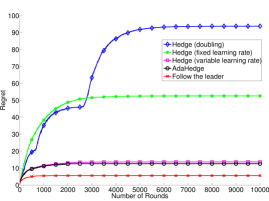
(a) I.I.D. losses

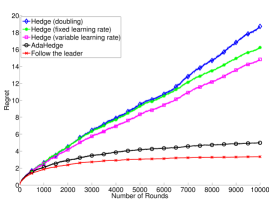
(b) Correlated losses

Figure 1: Simulation results

5.3 Discussion and Results

Figure 1 shows the results of the experiments above. We plot the regret (averaged over repetitions of the experiment) as a function of the number of rounds, for each of the considered algorithms.

I.I.D. Losses.

In the first considered regime, the accumulated losses for each action diverge linearly with high probability, so that the regret of Follow-the-Leader is bounded. Based on Theorem 9 we expect AdaHedge to incur bounded regret also; this is confirmed in Figure LABEL:fig:simlinear. Hedge with a fixed learning rate shows much larger regret. This happens because the learning rate, while it optimizes the worst-case bound, is much too small for this easy regime. In fact, if we would include more rounds, the learning rate would be set to an even smaller value, clearly showing the need to determine the learning rate adaptively. The doubling trick provides one way to adapt the learning rate; indeed, we observe that the regret of Hedge with the doubling trick is initially smaller than the regret of Hedge with fixed learning rate. However, unlike AdaHedge, the algorithm never detects that its current value of $\eta$ is working well; instead it keeps exhausting its budget, which leads to a sequence of clearly visible bumps in its regret. Finally, it appears that the Hedge algorithm with variable learning rate also achieves bounded regret. This is surprising, as the existing theory for this algorithm only considers its worst-case behaviour, and the algorithm was not designed to do specifically well in easy regimes.

Correlated Losses.

In the second simulation we investigate the case where the mean cumulative loss of two actions is extremely close — within $O(\log t)$ of one another. If the losses of the actions where independent, such a small difference would be dwarfed by random fluctuations in the cumulative losses, which would be of order $O(\sqrt{t})$. Thus the two actions can only be distinguished because we have made their losses dependent. Depending on the application, this may actually be a more natural scenario than complete independence as in the first simulation; for example, we can think of the losses as mistakes of two binary classifiers, say, two naive Bayes classifiers with different smoothing parameters. In such a scenario, losses will be dependent, and the difference in cumulative loss will be much smaller than $O(\sqrt{t})$. In the previous experiment, the posterior weights of the actions converged relatively quickly for a large range of learning rates, so that the exact value of the learning rate was most important at the start (e.g., from $3000$ rounds onward Hedge with fixed learning rate does not incur much additional regret any more). In this second setting, using a high learning rate remains important throughout. This explains why in this case Hedge with variable learning rate can no longer keep up with Follow-the-Leader. The results for AdaHedge are also interesting: although Theorem 9 does not apply in this case, we may still hope that $\Delta_{t}(\eta)$ grows slowly enough that the algorithm does not start too many segments. This turns out to be the case: over the $200$ repetitions of the experiment, AdaHedge started only $2.265$ segments on average, which explains its excellent performance in this simulation.

6 Proof of Lemma 6

Our main technical tool is Lemma 6. Its proof requires the following intermediate result:

Lemma 10.

For any $\eta>0$ and any time $t$, the function $f(\vloss_{t})=\ln\Big{(}\w_{t}\dot{e}^{-\eta\vloss_{t}}\Big{)}$ is convex.

This may be proved by observing that $f$ is the convex conjugate of the Kullback-Leibler divergence. An alternative proof based on log-convexity is provided in the Additional Material.

Proof of Lemma 6.

We need to bound $\delta_{t}=\w_{t}(\eta)\dot{\vloss}_{t}+\tfrac{1}{\eta}\ln(\w_{t}(\eta)\dot{e}^{-\eta\vloss_{t}})$, which is a convex function of $\vloss_{t}$ by Lemma 10. As a consequence, its maximum is achieved when $\vloss_{t}$ lies on the boundary of its domain, such that the losses $\ell_{t}^{k}$ are either $0$ or $1$ for all $k$, and in the remainder of the proof we will assume (without loss of generality) that this is the case. Now let $\alpha_{t}=\w_{t}\dot{\vloss}_{t}$ be the posterior probability of the actions with loss $1$. Then

$$\delta_{t}=\alpha_{t}+\frac{1}{\eta}\ln\left((1-\alpha_{t})+\alpha_{t}e^{-\eta}\right)=\alpha_{t}+\frac{1}{\eta}\ln\left(1+\alpha_{t}(e^{-\eta}-1)\right).$$

Using $\ln x\leq x-1$ and $e^{-\eta}\leq 1-\eta+\tfrac{1}{2}\eta^{2}$, we get $\delta_{t}\leq\tfrac{1}{2}\alpha_{t}\eta$, which is tight for $\alpha_{t}$ near $0$. For $\alpha_{t}$ near $1$, rewrite

$$\delta_{t}=\alpha_{t}-1+\frac{1}{\eta}\ln(e^{\eta}(1-\alpha_{t})+\alpha_{t})$$

and use $\ln x\leq x-1$ and $e^{\eta}\leq 1+\eta+(e-2)\eta^{2}$ for $\eta\leq 1$ to obtain $\delta_{t}\leq(e-2)(1-\alpha_{t})\eta$. Combining the bounds, we find

$$\delta_{t}\leq(e-2)\eta\min\{\alpha_{t},1-\alpha_{t}\}.$$

Now, let $k^{*}$ be an action such that $w_{t}^{*}=w_{t}^{k^{*}}$. Then $\ell^{k^{*}}_{t}=0$ implies $\alpha_{t}\leq 1-w_{t}^{*}$. On the other hand, if $\ell^{k^{*}}_{t}=1$, then $\alpha_{t}\geq w_{t}^{*}$ so $1-\alpha_{t}\leq 1-w_{t}^{*}$. Hence, in both cases $\min\{\alpha_{t},1-\alpha_{t}\}\leq 1-w_{t}^{*},$ which completes the proof. ∎

7 Conclusion and Future Work

We have presented a new algorithm, AdaHedge, that adapts to the difficulty of the DTOL learning problem. This difficulty was characterised in terms of convergence of the posterior probability of the best action. For hard instances of DTOL, for which the posterior does not converge, it was shown that the regret of AdaHedge is of the optimal order $O(\sqrt{L^{*}_{T}\ln(K)})$; for easy instances, for which the posterior converges sufficiently fast, the regret was bounded by a constant. This behaviour was confirmed in a simulation study, where the algorithm outperformed existing versions of Hedge.

A surprising observation in the experiments was the good performance of Hedge with a variable learning rate on some easy instances. It would be interesting to obtain matching theoretical guarantees, like those presented here for AdaHedge. A starting point might be to consider how fast the posterior probability of the best action converges to one, and plug that into Lemma 6.

Acknowledgments

The authors would like to thank Wojciech Kotłowski for useful discussions. This work was supported in part by the IST Programme of the European Community, under the PASCAL2 Network of Excellence, IST-2007-216886, and by NWO Rubicon grant 680-50-1010. This publication only reflects the authors’ views.

Appendix 0.A Additional Material

Proof of Lemma 2.

Lemma A.3 in [4] gives the bound $\ln\operatorname*{\mathbb{E}}[e^{sX}]\leq(e^{s}-1)\operatorname*{\mathbb{E}}[X]$ for any random variable $X$ taking values in $[0,1]$ and any $s\in\mathbb{R}$. Defining $X=\ell_{t}^{k}$ with distribution $\w_{t}$, setting $s=-\eta$ and dividing by the negative factor $(e^{-\eta}-1)$, we obtain

$$\frac{1}{e^{-\eta}-1}\ln(\w_{t}\dot{e}^{-\eta\vloss_{t}})\geq\w_{t}\dot{\vloss}_{t}.$$

It follows that

$$\Delta_{T}(\eta)=\sum_{t=1}^{T}\Big{(}\w_{t}\dot{\vloss}_{t}+\tfrac{1}{\eta}\ln(\w_{t}\dot{e}^{-\eta\vloss_{t}})\Big{)}\leq-f(\eta)\sum_{t=1}^{T}\ln(\w_{t}\dot{e}^{-\eta\vloss_{t}})=-f(\eta)\ln B_{T},$$

where $f(\eta)=1/(1-e^{-\eta})-1/\eta$ is a nonnegative, increasing function and $B_{T}$ is the marginal likelihood (see (1) and (2)). The lemma now follows by bounding $B_{T}$ from below by $\tfrac{1}{K}e^{-\eta L_{T}^{*}}$ and using $f(\eta)\leq f(1)=1/(e-1)$. ∎

Proof of Theorem 5.

In order to apply Lemma 4 we will need to bound the number of segments $m$. To this end, let $L^{*}(i)$ denote the cumulative loss of the best action on the $i$-th segment. That is, if the $i$-th segment spans rounds $t_{1},\ldots,t_{2}$, then $L^{*}(i)=\min_{k}\sum_{t=t_{1}}^{t_{2}}\ell_{t}^{k}$. If $m=1$, then the theorem is true by Lemma 4, so suppose that $m\geq 2$. Then we know that the budgets for the first $m-1$ segments have been depleted, so that for these segments (4) applies, giving:

$$\frac{\phi^{2m-2}-1}{\phi^{2}-1}=\sum_{i=1}^{m-1}\phi^{2i-2}=\sum_{i=1}^{m-1}\frac{1}{\eta_{i}^{2}}\leq\sum_{i=1}^{m-1}\frac{L^{*}(i)}{(e-1)\ln(K)}\leq\frac{L^{*}_{T}}{(e-1)\ln(K)}.$$

Solving for $m$, we find

$$m\leq\tfrac{1}{2}\log_{\phi}\Big{(}\frac{(\phi^{2}-1)L^{*}_{T}}{(e-1)\ln(K)}+1\Big{)}+1.$$

Substitution in Lemma 4 gives

$$R_{\text{AdaHedge}}(T) <2\ln(K)\Big{(}\frac{\phi^{m}-1}{\phi-1}\Big{)}+m\Big{(}\tfrac{1}{e-1}\ln(K)+\tfrac{1}{8}\Big{)}$$

$$=\frac{2\ln(K)}{\phi-1}\Big{(}\phi\sqrt{\frac{(\phi^{2}-1)L^{*}_{T}}{(e-1)\ln(K)}+1}-1\Big{)}+O\big{(}\ln(L^{*}_{T}+2)\ln(K)\big{)}$$

$$=\frac{2\ln(K)}{\phi-1}\phi\sqrt{\frac{(\phi^{2}-1)L^{*}_{T}}{(e-1)\ln(K)}}+O\big{(}\ln(L^{*}_{T}+2)\ln(K)\big{)},$$

where the last step uses $\sqrt{a+b}\leq\sqrt{a}+\sqrt{b}$. Rearranging yields the theorem. ∎

Proof of Lemma 7.

For $t$ between $\tau$ and $T$ we have

$$1/w^{*}_{t+1}(\eta)=\sum_{k=1}^{K}e^{-\eta(L^{k}_{t}-L^{*}_{t})}\leq 1+(K-1)e^{-\alpha\eta t^{\beta}},$$

which implies

$$\sum_{t=\tau}^{T}\big{(}1-w_{t+1}^{*}(\eta)\big{)} \leq\sum_{t=\tau}^{T}\Big{(}1-\frac{1}{1+(K-1)e^{-\alpha\eta t^{\beta}}}\Big{)}$$

$$=(K-1)\sum_{t=\tau}^{T}1/\big{(}e^{\alpha\eta t^{\beta}}+K-1\big{)}\leq(K-1)\sum_{t=\tau}^{\infty}e^{-\alpha\eta t^{\beta}}$$

$$\leq(K-1)\int_{0}^{\infty}e^{-\alpha\eta t^{\beta}}\,\textnormal{d}t=(K-1)(\alpha\eta)^{-1/\beta}\Gamma(1+1/\beta),$$

where the integral can be evaluated using the variable substitution $u=\alpha\eta t^{\beta}$ and the fact that $z\Gamma(z)=\Gamma(1+z)$. ∎

Proof of Lemma 8.

Let

$$\Delta_{T}(m^{*},\eta)=\sum_{t=s(m^{*})}^{T}\Big{(}\w_{t}(\eta)\dot{\vloss}_{t}+\tfrac{1}{\eta}\ln(\w_{t}(\eta)\dot{e}^{-\eta\vloss_{t}})\Big{)}$$

be a version of $\Delta_{T}(\eta)$ measured only on the rounds since the start of the $m^{*}$-th segment. We bound the first $\tau-1$ terms in this sum using Lemma 1 and the remaining terms using Lemmas 6 and 7, which gives

$$\Delta_{T}(m^{*},\eta) =\sum_{t=s(m^{*})}^{T}\Big{(}\delta_{t}(\eta)\Big{)}$$

$$\leq\frac{(\tau-1)\eta}{8}+(e-2)C_{K}\eta^{1-1/\beta}\leq\frac{1}{8}\big{(}\tau-1+8(e-2)C_{K}\big{)}\eta^{1-1/\beta}$$

for any $\eta\leq 1$.

We will argue that the budget in segment $m^{*}$ is never depleted: $\Delta_{T}(m^{*},\eta_{m^{*}})<b(\eta_{m^{*}})=\ln(K)/\eta_{m^{*}}+\ln(K)/(e-1)$, for which it is sufficient to show that

$$\frac{1}{8}\big{(}\tau-1+8(e-2)C_{K}\big{)}\eta_{m^{*}}^{1-1/\beta} \leq\frac{\ln(K)}{\eta_{m^{*}}}$$

$$\tau \leq 8\ln(K)\eta_{m^{*}}^{1/\beta-2}-8(e-2)C_{K}+1$$

$$=8\ln(K)\phi^{(m^{*}-1)(2-1/\beta)}-8(e-2)C_{K}+1,$$

which is true by definition of $\tau$. ∎

Proof of Theorem 9.

We will show that the conditions of Lemma 8 (with the same $\alpha$, and $\beta=1$) are satisfied with probability at least $1-\delta$. For $r=\tau,\tau+1,\ldots$, let $A_{r}^{k}$ denote the event that $L_{r}^{k}(m^{*})-\operatorname*{\mathbb{E}}[L_{r}^{k}(m^{*})]\geq-\tfrac{\alpha}{2}r$ for $k\neq k^{*}$, let $B_{r}$ denote the event that $L_{r}^{k^{*}}(m^{*})-\operatorname*{\mathbb{E}}[L_{r}^{k^{*}}(m^{*})]\leq\tfrac{\alpha}{2}r$, and let $D_{r}=B_{r}\cap\bigcap_{k\neq k^{*}}A_{r}^{k}$ denote the intersection of these events. Using (7), it can be seen that $L_{r}^{k}-L_{r}^{k^{*}}\geq\alpha r$ on $D_{r}$, as required by (6). Hence we need to show that the probability of $\bigcap_{r\geq\tau}D_{r}$ is at least $1-\delta$, or equivalently that the probability of the complementary event $\bigcup_{r\geq\tau}\bar{D}_{r}$ is at most $\delta$.

By Hoeffding’s inequality [4] the probabilities of the complementary events $\bar{A}_{r}^{k}$ and $\bar{B}_{r}$ may each be bounded by $\exp(-\tfrac{1}{2}\alpha^{2}r)$. And hence by the union bound the probability of $\bar{D}_{r}$ is bounded by $K\exp(-\tfrac{1}{2}\alpha^{2}r)$. Again by the union bound it follows that

$$\Pr\Big{(}\bigcup_{r\geq\tau}\bar{D}_{r}\Big{)}\leq\sum_{r=\tau}^{\infty}Ke^{-\tfrac{1}{2}\alpha^{2}r}\leq K\int_{\tau-1}^{\infty}e^{-\tfrac{1}{2}\alpha^{2}r}\,\textnormal{d}r\\ =\tfrac{2K}{\alpha^{2}}e^{-\tfrac{1}{2}\alpha^{2}(\tau-1)}.$$

We require this probability to be bounded by $\delta$, for which it is sufficient that

$$\tau\geq\frac{2}{\alpha^{2}}\ln\Big{(}\frac{2K}{\alpha^{2}\delta}\Big{)}+1.$$ (10)

By definition of $\tau$, this is implied by

$$8\ln(K)\phi^{m^{*}-1}-\tfrac{8(K-1)(e-2)}{\alpha} \geq\frac{2}{\alpha^{2}}\ln\Big{(}\frac{2K}{\alpha^{2}\delta}\Big{)}+1,$$

which holds for our choice (8) of $m^{*}$. To show that AdaHedge starts at most $m^{*}$ segments, it remains to verify the other condition of Lemma 8, which is that $\tau\geq 1$. This follows from (10) upon observing that (7) implies $\alpha\leq\tfrac{1}{2}$ so that $\frac{2}{\alpha^{2}}\ln\Big{(}\frac{2K}{\alpha^{2}\delta}\Big{)}\geq 0$.

Finally, the bound on the regret is obtained by plugging $m^{*}$ into Lemma 4. ∎

Proof of Lemma 10.

Within this proof, let us drop the subscript $t$ from $\vloss_{t}$ and $\w_{t}$, and define the function $f_{k}(\vloss)=e^{-\eta\ell^{k}}$ for every action $k$. Let $\vloss_{0}$ and $\vloss_{0}$ be arbitrary loss vectors, and let $\lambda\in(0,1)$ also be arbitrary. Then it is sufficient to show that

$$\ln\operatorname*{\mathbb{E}}_{k\sim\w}[f_{k}(\vloss_{\lambda})]\leq(1-\lambda)\ln\operatorname*{\mathbb{E}}_{k\sim\w}[f_{k}(\vloss_{0})]+\lambda\ln\operatorname*{\mathbb{E}}_{k\sim\w}[f_{k}(\vloss_{1})],$$ (11)

where $\vloss_{\lambda}=(1-\lambda)\vloss_{0}+\lambda\vloss_{1}$. Towards this end, we start by observing that $f_{k}$ is log-convex:

$$\ln f_{k}(\vloss_{\lambda})\leq(1-\lambda)\ln f_{k}(\vloss_{0})+\lambda\ln f_{k}(\vloss_{1}).$$ (12)

Inequality 11 now follows from the general fact that a convex combination of log-convex functions is itself log-convex, which we will proceed to prove: using first (12) and then applying Hölder’s inequality (see e.g. [11]) one obtains

$$\operatorname*{\mathbb{E}}_{k\sim\w}[f_{k}(\vloss_{\lambda})]\leq\operatorname*{\mathbb{E}}_{k\sim\w}\big{[}f_{k}(\vloss_{0})^{1-\lambda}f_{k}(\vloss_{1})^{\lambda}\big{]}\leq\operatorname*{\mathbb{E}}_{k\sim\w}[f_{k}(\vloss_{0})]^{1-\lambda}\operatorname*{\mathbb{E}}_{k\sim\w}[f_{k}(\vloss_{1})]^{\lambda},$$

from which (11) follows by taking natural logarithms. ∎

References

- [1] Y. Freund and R. E. Schapire. A decision-theoretic generalization of on-line learning and an application to boosting. Journal of Computer and System Sciences, 55:119–139, 1997.
- [2] N. Littlestone and M. K. Warmuth. The weighted majority algorithm. Information and Computation, 108(2):212–261, 1994.
- [3] V. Vovk. A game of prediction with expert advice. Journal of Computer and System Sciences, 56(2):153–173, 1998.
- [4] N. Cesa-Bianchi and G. Lugosi. Prediction, learning, and games. Cambridge University Press, 2006.
- [5] Y. Freund and R. E. Schapire. Adaptive game playing using multiplicative weights. Games and Economic Behavior, 29:79–103, 1999.
- [6] E. Hazan and S. Kale. Extracting certainty from uncertainty: Regret bounded by variation in costs. In Proceedings of the 21st Annual Conference on Learning Theory (COLT), pages 57–67, 2008.
- [7] N. Cesa-Bianchi, Y. Freund, D. Haussler, D. P. Helmbold, R. E. Schapire, and M. K. Warmuth. How to use expert advice. Journal of the ACM, 44(3):427–485, 1997.
- [8] P. Auer, N. Cesa-Bianchi, and C. Gentile. Adaptive and self-confident on-line learning algorithms. Journal of Computer and System Sciences, 64:48–75, 2002.
- [9] V. Vovk. Competitive on-line statistics. International Statistical Review, 69(2):213–248, 2001.
- [10] D. Haussler, J. Kivinen, and M. K. Warmuth. Sequential prediction of individual sequences under general loss functions. IEEE Transactions on Information Theory, 44(5):1906–1925, 1998.
- [11] A. N. Shiryaev. Probability. Springer-Verlag, 1996.