The Hubble Space Telescope Cluster Supernova Survey:
VI. The Volumetric Type Ia Supernova Rate

Abstract

We present a measurement of the volumetric Type Ia supernova (SN Ia) rate out to $z\simeq 1.6$ from the Hubble Space Telescope Cluster Supernova Survey. In observations spanning 189 orbits with the Advanced Camera for Surveys we discovered 29 SNe, of which approximately 20 are SNe Ia. Twelve of these SNe Ia are located in the foregrounds and backgrounds of the clusters targeted in the survey. Using these new data, we derive the volumetric SN Ia rate in four broad redshift bins, finding results consistent with previous measurements at $z\gtrsim 1$ and strengthening the case for a SN Ia rate that is $\gtrsim$$0.6\times 10^{-4}h_{70}^{3}$ yr^-1 Mpc^-3 at $z\sim 1$ and flattening out at higher redshift. We provide SN candidates and efficiency calculations in a form that makes it easy to rebin and combine these results with other measurements for increased statistics. Finally, we compare the assumptions about host-galaxy dust extinction used in different high-redshift rate measurements, finding that different assumptions may induce significant systematic differences between measurements.

1. Introduction

Type Ia supernovae (SNe Ia) are of great importance both as astrophysical objects and as cosmological distance indicators. An accurate knowledge of the rate at which they occur (as a function of redshift) is essential for understanding both of these roles. Astrophysically, SNe Ia play an important role in galaxy evolution. They are a major source of iron (e.g., Matteucci & Greggio, 1986; Tsujimoto et al., 1995; Thielemann et al., 1996) and inject energy into the interstellar medium (e.g., Dekel & Silk, 1986; Scannapieco et al., 2006). The SN Ia rate is necessary to include these effects in galaxy evolution models, particularly at high redshifts where much of the important galaxy evolution occurs. Cosmologically, SNe Ia are the best-tested method for measuring the scale factor of the universe as a function of redshift, with hundreds of SNe now employed in the precision measurement of cosmological parameters (e.g., Hicken et al., 2009; Amanullah et al., 2010; Sullivan et al., 2011). Despite their widespread use as distance indicators, the process that leads to a SN Ia is still not well understood. SNe Ia are widely accepted to be the end result of a carbon-oxygen (CO) white dwarf (WD) nearing the Chandrasekhar mass limit but how they near that limit is not known (see Livio, 2001, for a review). This leaves open the question of whether high-redshift SNe are different from low-redshift SNe in a way that affects the inferred distance.

Measurements of the change in the SN Ia rate with redshift can be used to distinguish between models of how SNe Ia occur. While there are a variety of SN Ia progenitor models, most fall into two classes: the single degenerate scenario (SD; Whelan & Iben, 1973) and the double degenerate scenario (DD; Iben & Tutukov, 1984; Webbink, 1984). In the single degenerate scenario, the WD accretes mass from a red giant or main sequence star that overflows its Roche lobe. In the double degenerate scenario, the WD merges with a second white dwarf after orbital decay due to the emission of gravitational radiation. Crucially, the delay time between the initial formation of the system and the SN explosion is governed by a different physical mechanism in the different models. This allows us to differentiate between models by measuring the distribution of the delay times for a population of SNe. The shape of this delay time distribution (DTD) depends on the details of the binary star evolution (particularly its evolution through one or more common envelope phases) and the specific progenitor model. One method for measuring the DTD is to correlate the cosmic star formation history (SFH) with the the cosmic SN Ia rate as a function of redshift (Yungelson & Livio, 2000): the rate as a function of cosmic time is simply the cosmic SFH convolved with the DTD.

The volumetric SN Ia rate has now been measured in many different SN surveys designed to detect and measure SNe at $z<1$ (e.g. Pain et al., 2002; Neill et al., 2007; Dilday et al., 2010). With the recently revised rates from the IfA Deep survey (Rodney & Tonry, 2010), most of these $z<1$ measurements have now come into agreement. In contrast, measurements at $z>1$ have been limited to SN searches in the GOODS fields (Dahlen et al., 2004; Kuznetsova et al., 2008; Dahlen et al., 2008) using the Hubble Space Telescope (HST) and ultra-deep single-epoch searches in the Subaru Deep Field (SDF) from the ground (Poznanski et al., 2007; Graur et al., 2011). These studies have yielded discrepant results for the DTD. The first $z>1$ measurements by Dahlen et al. (2004) (and later Dahlen et al., 2008, with an expanded dataset) showed a rate that peaked at $z\sim 1$ and decreased in the highest-redshift bin at $z>1.4$. From these results the best-fit DTD is one tightly confined to 3–4 Gyr with very few SNe Ia having short delay times (Strolger et al., 2010). The recent results of Graur et al. (2011) from the SDF show a lower rate at $z\sim 1$, and a higher rate in the highest-redshift bin compared with Dahlen et al. (2008). These results are consistent with a flat SN rate at $1<z<2$. They find that the DTD is consistent with a power law with the best-fit $\propto t^{-1.1}$, implying a significant fraction of short delay time ($\lesssim 1$ Gyr) SNe.

Relative to the HST measurements, the SDF measurements cover a much larger volume and therefore have the advantage of better statistics in the highest-redshift bin, but HST measurements hold advantages in systematics. A rolling search with HST offers multiple observations of each SN and much higher resolution than possible from the ground, useful for resolving SNe from the cores of their hosts. These factors lead to a more robust identification of SNe Ia relative to the SDF searches where a single observation is used for both detection and photometric typing. In addition, the Dahlen et al. (2008) analysis used spectroscopic typing in addition to photometric typing, whereas Graur et al. (2011) uses only photometric typing. In general, the very different strategies employed make HST measurements a good cross-check for the SDF measurements and vice versa. Increasing the statistics in HST rate measurements can make this cross-check better and improve DTD constraints. At the same time, in comparing the measurements it is important to carefully consider possible systematic differences, particularly as statistical uncertainty decreases and systematics come to dominate.

In this paper, we address these issues by (1) supplementing current determinations of the HST-based $z\gtrsim 1$ SN Ia rate and (2) comparing the effect on results of different dust distributions assumed in previous analyses. We use observations from the HST Cluster Supernova Survey, a survey to discover and follow SNe Ia in very distant clusters (Dawson et al., 2009, PI: Perlmutter, GO-10496). The survey encompassed 189 orbits with the Advanced Camera for Surveys (ACS) over a period of 18 months. The SN selection and SN typing for the all SNe in the survey was presented in Barbary et al. (2011, hereafter B11), where we calculated the cluster SN Ia rate from the survey. Here, we use a similar methodology to B11 but focus on the SNe discovered in the cluster foregrounds and backgrounds. The remainder of the paper is organized as follows: In §2 we summarize the HST Cluster Supernova Survey and the SN discoveries. In §3 we describe the Monte Carlo simulation used to calculate a rate based on the SN discoveries. In §4 we present results and characterize systematic uncertainties. Finally, in §5 we compare our results to published measurements. Throughout the paper we use a cosmology with $H_{0}=70$ km s^-1 Mpc^-1, $\Omega_{M}=0.3$, $\Omega_{\Lambda}=0.7$. Magnitudes are in the Vega system.

This paper is one of a series of ten papers (Melbourne et al., 2007; Barbary et al., 2009; Dawson et al., 2009; Morokuma et al., 2010; Suzuki et al., 2011; Ripoche et al., 2011; Meyers et al., 2011; Hsiao et al., 2011, B11; This work) that report supernova results from the HST Cluster Supernova Survey. The survey strategy and SN discoveries are described in Dawson et al. (2009), while spectroscopic follow-up observations for SN candidates are presented in Morokuma et al. (2010). A separate series of papers, ten to date, reports on cluster studies from the survey: Hilton et al. (2007); Eisenhardt et al. (2008); Jee et al. (2009); Hilton et al. (2009); Huang et al. (2009); Rosati et al. (2009); Santos et al. (2009); Strazzullo et al. (2010); Brodwin et al. (2011); Jee et al. (2011).

2. Survey and Supernova Discoveries

The details of the HST Cluster SN Survey are described in Dawson et al. (2009). Briefly, the survey targeted 25 massive galaxy clusters in a rolling SN search between July 2005 and December 2006. Clusters were selected from X-ray, optical and IR surveys and cover the redshift range $0.9<z<1.46$. During the survey, each cluster was observed once every 20 to 26 days during its HST visibility window (typically four to seven months) using ACS. Each visit consisted of four exposures in the F850LP filter (hereafter $z_{850}$). Most visits also included a fifth exposure in the F775W filter (hereafter $i_{775}$).

Table 1Non-Cluster Supernova Discoveries

ID	Nickname	$z$	Cluster $z$	Type	Confidence
SNe: Not in Clusters
SN SCP06L21	$\cdots$	$\cdots$	1.37	CC	plausible
SN SCP05N10	Tobias	0.203	1.03	CC	plausible
SN SCP06C7	$\cdots$	0.610	0.97	CC	probable
SN SCP06Z5	Adrian	0.623	1.39	Ia	secure
SN SCP06B3	Isabella	0.743	1.12	CC	probable
SN SCP06F8	Ayako	0.789	1.11	CC	probable
SN SCP05P9	Lauren	0.821	1.10	Ia	secure
SN SCP06H3	Elizabeth	0.850	1.24	Ia	secure
SN SCP06U7	Ingvar	0.892	1.04	CC	probable
SN SCP05P1	Gabe	0.926	1.10	Ia	probable
SN SCP06G3	Brian	0.962	1.26	Ia	plausible
SN SCP06C0	Noa	1.092	0.97	Ia	secure
SN SCP06N33	Naima	1.188	1.03	Ia	probable
SN SCP06F6	$\cdots$	1.189	1.11	non-Ia	secure
SN SCP06A4	Aki	1.193	1.46	Ia	probable
SN SCP05D6	Maggie	1.314	1.02	Ia	secure
SN SCP06G4	Shaya	1.350	1.26	Ia	secure
SN SCP06X26	Joe	1.44?	1.10	Ia	plausible
SNe: Cluster Membership Uncertain
SN SCP06E12	Ashley	$\cdots$	1.03	Ia	plausible
SN SCP06N32	$\cdots$	$\cdots$	1.03	CC	plausible
Uncertain to be SN
SN SCP06M50	$\cdots$	$\cdots$	0.90	$\cdots$	$\cdots$

The process of selecting SN Ia candidates for the rates analysis is described in detail in B11. We briefly summarize it here. Candidates were detected in subtractions of $z_{850}$ images and examined by eye to eliminate obviously false detections such as stellar diffraction spikes. A total of 86 candidates were selected in this phase. Detailed information on all 86 of these candidates is available from the survey website. We generated a full light curve in $z_{850}$ and $i_{775}$ for each of these candidates and then imposed automated requirements on the light curve. These included a requirement on the flux in $i_{775}$ and the rapidity of the rise and fall of the light curve. After this step, 60 SN candidates remained. (The selections up to this point are accounted for in our calculation of detection efficiency.) The remaining candidates were then divided into image artifacts (14), AGN (17), and supernovae (29) on the basis of the light curve shape and evidence from image subtractions. For example, candidates on the cores of bright galaxies and showing adjoining positive and negative regions in image subtractions are likely to be the result of image mis-alignment. With corroborating evidence from the light curves of such candidates, they are confidently dismissed as image artifacts. Similarly, candidates deemed to be AGN were located on the cores of galaxies and exhibited light curves that look nothing like SNe light curves: most rose or fell over periods of 100+ days. In general, the continuous light curve monitoring in the survey made possible to separate these artifacts and AGN from SNe with high confidence. For the remaining 29 candidates deemed to be SNe, we determined a SN type and confidence for each. In Table 1 we list the SNe along with their host galaxy redshifts, SN types and confidence. We omit the eight SNe whose hosts are spectroscopically confirmed cluster members. See Figure 4 of B11 for images, light curves and light curve fits of all candidates. A complete description of the SN coordinates, typing and confidence level (plausible, probable, or secure) is given in B11. Briefly, a secure SN Ia has either spectroscopic confirmation, or evidence from two sources (early-type host galaxy and light curve) ruling out other types. A probable SN Ia is slightly less certain than a secure SN Ia, but still a high-confidence SN Ia: the light curve rules out all core collapse subtypes. A plausible SN Ia has a light curve that is more indicative of a SN Ia than SN CC, but is not sufficient to rule out all core-collapse types.

In this analysis we use two additional selections not used in B11: (1) First, we eliminate candidates that could only be consistent with a SN Ia if it peaked prior to 10 rest-frame days before the first observation. We found that lower-redshift ($z\lesssim 0.9$) SNe were detectable even when peaking well before the first observation, but that such SNe were extremely difficult to type as they were observed only far into the light curve decline. We found it most “fair” to eliminate such candidates entirely. We include the same selection in our efficiency simulations below. Only SCP06L21 and SCP05N10 are rejected based on this selection, but both are below the redshift range of greatest interest ($z>0.6$) and at least SCP05N10 is incompatible with an SN Ia light curve anyway. This was not an issue for B11 because SNe of interest (at $z\geq 0.9$) are not detectable very far after peak.

(2) Second, we exclude regions within $20^{\prime\prime}$ of cluster centers, in order to avoid the most strongly lensed areas in the volume behind the clusters. This region is only $\sim$$3\%$ of the observed field of each cluster. Note that we were careful to choose this radius before looking at the radii of any of the candidates, in order to avoid biasing ourselves by adjusting the radius to conveniently exclude or include candidates. Two candidates were excluded as a result: SNe SCP06B3 ($16.8^{\prime\prime}$ from the cluster center) and SCP06M50 ($19.4^{\prime\prime}$ from the cluster center). As it happens, these candidates are unlikely to be SNe Ia. SN SCP06B3 is a “probable” SN CC, while SN SCP06M50 is possibly not a SN at all and may be hosted by a cluster member galaxy, making its position near the cluster center unsurprising. The exclusion of this region is taken into account in our simulations (§3). The effect of lensing on the remaining portions of the fields are discussed in §4.2.

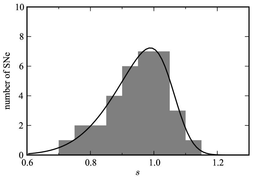
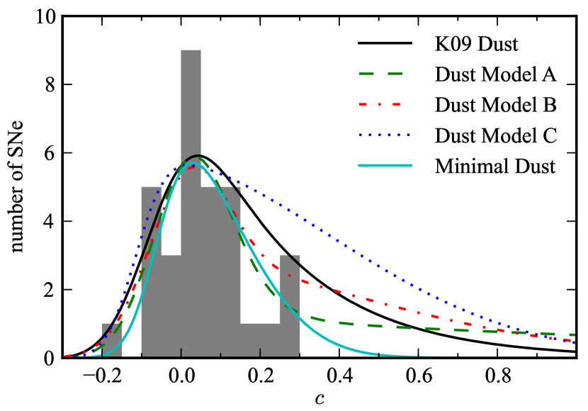
Figure 1.— Left Panel: Stretch distribution used for simulated SNe (solid black line) and the stretch distribution of first-year SNLS $z<0.6$ SNe (grey histogram) from Astier et al. (2006). Right Panel: Color distribution used for simulated SNe (solid black line), based on the K09 distribution of host-galaxy extinction. The grey histogram shows the color distribution of the first-year SNLS $z<0.6$ SNe. The other four lines show alternative color distributions used to assess the possible systematic uncertainty due to different distributions of host galaxy dust extinction (see §4.3).

The systematic uncertainties associated with the determination of SN type and redshift for the remaining candidates are addressed in §4.1.

3. Rate Calculation

We calculate the SN Ia rate in redshift bins using what has become a standard method in rate calculations: The number of SNe Ia per unit time per comoving volume is estimated in the redshift bin $z_{1}<z<z_{2}$ by

$$\mathcal{R}(z_{1}<z<z_{2})=\frac{N_{\rm SN~{}Ia}(z_{1}<z<z_{2})}{\int_{z_{1}}^{z_{2}}T(z)\frac{1}{1+z}\frac{\Theta}{4\pi}\frac{dV}{dz}(z)dz}$$ (1)

where $N_{\rm SN~{}Ia}(z_{1}<z<z_{2})$ is the number of SNe Ia discovered between redshifts $z_{1}$ and $z_{2}$, and the denominator is the total effective time-volume for which the survey is sensitive to SNe Ia in the redshift range $z_{1}<z<z_{2}$. $T(z)$ is the effective visibility time (also known as the “control time”) and is calculated by integrating the probability of detecting a SN Ia as a function of time over the active time of the survey. $T(z)$ depends on the dates and depths of observations, as well as the specific requirements for selecting SNe. The factor of $1/(1+z)$ converts from observer-frame time to rest-frame time at redshift $z$. The last two terms in the denominator represent the volume comoving element between $z$ and $z+dz$ observed in the survey. $\frac{dV}{dz}(z)$ is the comoving volume of a spherical shell of width $dz$. $\Theta$ is the solid angle observed in the survey, in units of steradians. ($\Theta/4\pi$ is the fraction of the spherical shell we have observed.) Finally, the average redshift of the bin, weighted by the volume effectively observed, is given by

$$\bar{z}=\frac{\int_{z_{1}}^{z_{2}}zT(z)\frac{1}{1+z}\frac{dV}{dz}(z)dz}{\int_{z_{1}}^{z_{2}}T(z)\frac{1}{1+z}\frac{dV}{dz}(z)dz}.$$ (2)

As in B11, we use an effective visibility time that depends on position, as observation dates and depths vary within each observed field. That is, in Equation (1) we make the substitution

$$T(z)\Theta\Rightarrow\int_{x,y}T(x,y,z)dxdy.$$ (3)

$T(x,y,z)$ is calculated by simulating SN Ia light curves at different positions, redshifts and times during the survey, and determining the probability that each simulated SN would be detected and counted in our SN sample. We pass each simulated SN through the same automated selections used to select the 60 candidates in our initial sample. Additionally, we discard simulated SNe peaking prior to 10 rest-frame days before the first observation, as discussed in the previous section.

We characterize the diversity of SN Ia light curves as a two-parameter family (stretch $s$ and color $c$) with an additional intrinsic dispersion in luminosity. The absolute magnitude of each simulated SN is set to

$$M_{B}=-19.31-\alpha(s-1)+\beta c+I$$ (4)

where $-19.31$ is the magnitude of an $s=1$, $c=0$ SN Ia in our assumed cosmology (Astier et al., 2006), $\alpha=1.24$, $\beta=2.28$ (Kowalski et al., 2008), and $I$ is an added “intrinsic dispersion”, randomly drawn from a Gaussian distribution centered at zero with $\sigma=0.15$ mag, as seen in Kowalski et al. (2008). This produces a set of simulated SNe that closely matches the distribution seen in Kowalski et al. (2008). To calculate the flux of each simulated SN in the observed $z_{850}$ and $i_{775}$ filters, we use the Hsiao et al. (2007) spectral time series template.

The main difference from B11 is that we use distributions for stretch and color that are representative of SNe in the field rather than in clusters. For stretch, we look to the observed stretch distribution of the first-year sample from the Supernova Legacy Survey (SNLS; Astier et al., 2006), cut at $z<0.6$ to limit Malmquist bias (Figure 1, grey histogram). We assume this sample is complete, fit a smooth curve to the distribution (same panel, solid line), and use this for simulated SNe.

For color, we cannot assume the SNLS sample (Figure 1, histogram in right panel) is complete even at $z<0.6$, as highly reddened SNe will have been missed. The standard picture today is that the observed distribution of SN colors is due to a combination of both intrinsic SN color variation and host galaxy extinction (Guy et al., 2010; Chotard et al., 2011). Both of these are expected to introduce a color that correlates with SN luminosity, possibly with different strengths ($\beta$ is typically found to be smaller than the canonical value of $R_{B}=4.1$ for Milky Way dust). In order to capture both effects with a single color distribution and a single $\beta$, we work backwards from the desired host galaxy extinction distribution. We wish to achieve a host galaxy extinction distribution of $P(A_{V})\propto\exp(-A_{V}/0.33)$ with $A_{V}\geq 0$, the best-fit value for host-galaxy SN extinction in the SDSS-II SN Survey (Kessler et al., 2009, hereafter K09). To do this we use a color distribution of $P(c)\propto\exp(-(\beta-1)c/0.33)$, because $A_{V}$ is related to $c$ via $A_{V}=R_{V}\times E(B-V)\approx(\beta-1)\times c$. This ensures the desired $A_{V}$ distribution is obtained for any given value of $\beta$. The full $P(c)$ distribution is then a convolution of this $P(c)$ distribution from host galaxy dust and the intrinsic distribution of SN color (assumed to be Gaussian). The Gaussian parameters of the intrinsic distribution are chosen so that the full convolved $P(c)$ distribution matches the observed SNLS $c$ distribution at $c<0.3$. The result is a $P(c)$ distribution (black line in right panel of Figure 1) that matches the SNLS sample where we expect it to be complete ($c<0.3$) and also has the desired behavior at large extinction based on our assumed $P(A_{V})$ distribution. We use this distribution in our simulation. In §4.3 we assess the systematic uncertainty associated with host galaxy dust by using alternate color distributions obtained using the same method, but different $P(A_{V})$ distributions (other curves in the same panel).

$T(x,y,z)$ is calculated in bins of 100 $\times$ 100 pixels ($5^{\prime\prime}\ \times\ 5^{\prime\prime}$) in position. In each $5^{\prime\prime}\ \times\ 5^{\prime\prime}$ region, we simulate 50 SN light curves with random parameters and random position (within the bin) and take the average effective visibility time of the 50 SNe ($\sim$80,000 SNe per field). Summing over all areas observed in all 25 fields yields $T(z)$. In doing so we exclude regions within $20^{\prime\prime}$ of cluster centers, as discussed in the previous section. We calculate $T(z)$ at intervals of $\Delta z=0.05$ in redshift.

4. Results and Systematic Uncertainty

Figure 2 (top panel, black line) shows the product of the observer-frame effective visibility time and the area ($T(z)\Theta$ from Eq. 1) as a function of SN redshift. For reference, the horizontal dotted line shows an approximate calculation of this value, multiplying the area of the ACS field (11.65 arcmin²) by the time difference between 10 days before the first observation and 10 days after the last observation. In reality the area actually observed is slightly more complicated and SNe are detected over a slightly larger time range. From $z=0$, the effective visibility time actually increases slightly out to $z\sim 0.5$ as SN light curves are time-dilated and are thus visible for longer. Afterwards, we begin to miss SNe that peak during the observations. In the lower panel of Figure 2, we convert to the rest-frame time-volume observed in each redshift bin of $\Delta z=0.05$ using the assumed cosmology.

Table 2 shows the results, in bins of $\Delta z=0.4$ (comparable to Dahlen et al., 2008) and also in bins of $\Delta z=0.5$ (comparable to Graur et al., 2011). The numerator of Equation (1) (third column in Table 2) is the number of SNe Ia described in §2. The denominator of Equation (1) (fourth column in Table 2) is obtained by summing Figure 2 (lower panel) over the redshift bin of interest. We now discuss the systematic uncertainties associated with lensing, SN type determination, host-galaxy dust, SN properties, and galaxy number density variations.

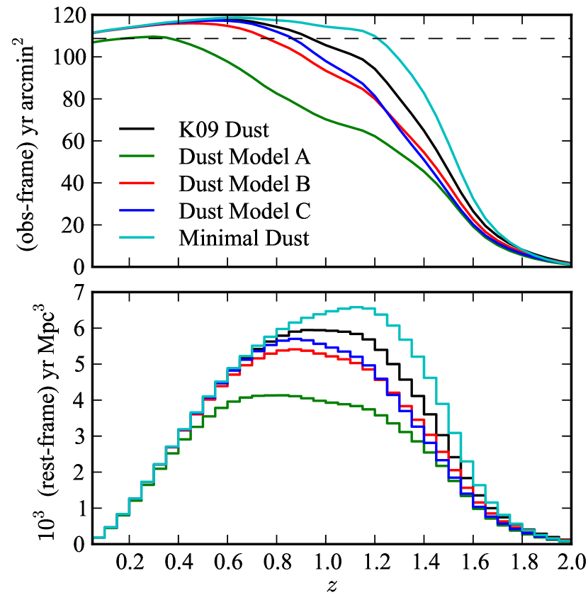
Figure 2.— Top Panel: The observer-frame effective visibility time multiplied by observed area, as a function of supernova redshift. The horizontal dotted line shows the area of the ACS field multiplied by the time spanned by the observations in each cluster. Bottom Panel: The rest-frame volume-time searched in each redshift bin of $\Delta z=0.05$. In each panel, the black line shows our main result for the effective visibility time, based on simulations using the K09 dust distribution. The green, red, blue and cyan lines show the results for alternative dust distributions. [Data in this figure is available as a machine-readable table.]

4.1. Type determination

The uncertainty in SN type in the survey is quite small, thanks to the cadenced nature of the survey and excellent spectroscopic follow-up. Consider the candidates designated as SN Ia: all three SNe Ia at $z<0.9$ are spectroscopically confirmed. At $z\gtrsim 0.9$, any SN bright enough to be detected is overwhelmingly likely to be Type Ia due to the faintness of core-collapse SNe relative to SNe Ia (e.g., Dahlen et al., 2004; Li et al., 2011; Meyers et al., 2011). Furthermore, while “probable” candidates are not as certain as “secure” candidates, this is still a fairly high-confidence type determination: A “probable” SN Ia means that a SN Ia light curve template has a $\chi^{2}$ $P$-value that is $10^{3}$ times larger than any SN CC value. A Bayesian analysis would therefore yield a type uncertainty close to zero for such candidates, regardless of the prior used.

Table 2Results: SN Ia Rate

Redshift bin	$\bar{z}$	$N_{\rm SN~{}Ia}$	Denom	Rate
bin width $\Delta z=0.4$
$0.2<z\leq 0.6$	0.442	$0.00^{+1.16+0.00}_{-0.00-0.00}$	2.332	$0.00^{+0.50+0.00}_{-0.00-0.00}$
$0.6<z\leq 1.0$	0.807	$5.25^{+2.69+0.25}_{-2.00-1.25}$	4.464	$1.18^{+0.60+0.44}_{-0.45-0.28}$
$1.0<z\leq 1.4$	1.187	$5.63^{+2.77+0.63}_{-2.08-0.63}$	4.243	$1.33^{+0.65+0.69}_{-0.49-0.26}$
$1.4<z\leq 1.8$	1.535	$1.12^{+1.56+0.12}_{-0.79-1.12}$	1.453	$0.77^{+1.07+0.44}_{-0.54-0.77}$
bin width $\Delta z=0.5$
$0.0<z\leq 0.5$	0.357	$0.00^{+1.16+0.00}_{-0.00-0.00}$	1.624	$0.00^{+0.71+0.00}_{-0.00-0.00}$
$0.5<z\leq 1.0$	0.766	$5.25^{+2.69+0.25}_{-2.00-1.25}$	5.321	$0.99^{+0.51+0.33}_{-0.38-0.24}$
$1.0<z\leq 1.5$	1.222	$6.75^{+2.99+0.75}_{-2.31-1.75}$	4.906	$1.38^{+0.61+0.71}_{-0.47-0.43}$
$1.5<z\leq 2.0$	1.639	$0.00^{+1.16+0.00}_{-0.00-0.00}$	0.890	$0.00^{+1.30+0.00}_{-0.00-0.00}$

Table 3SN Rate Uncertainties in Percentage

		statistical		systematic
Redshift bin		Poisson		Typing	Dust	Luminosity
$0.6<z\leq 1.0$		+51/$-$38		+4/$-$23	+37/$-$3	+2/$-$2
$1.0<z\leq 1.4$		+49/$-$36		+11/$-$11	+49/$-$14	+10/$-$7
$1.4<z\leq 1.8$		+138/$-$69		+11/$-$100	+39/$-$19	+38/$-$23

Note. — Percentages are not reported for the $0.2<z<0.6$ bin because there were no SNe detected in this bin.

The “plausible” candidates are perhaps the only candidates with significant type uncertainty. It is difficult to precisely quantify this uncertainty. Instead, we provide conservative bounds in a manner similar to Dahlen et al. (2008) and Sharon et al. (2010): we first assign a lower limit to the number of SNe Ia discoveries by assuming that all “plausible” SNe Ia are in fact SNe CC. We then assign an upper limit by assuming that all “plausible” SNe CC are in fact SNe Ia. These limits are shown in Table 2 as the second confidence interval for $N_{\rm SN~{}Ia}$. The corresponding systematic uncertainty in the SN rate is shown in Table 3.

For the two candidates without spectroscopic host redshifts, we assign a redshift range consistent with the SN light curve and/or host galaxy photometry, as follows: For SCP06E12, we use the range $0.8<z<1.2$. As there is uncertainty about both the type and cluster membership, we count SCP06E12 as $0.5\pm 0.5$ field SNe Ia. The situation is similar for SCP06N32: the light curve is consistent with an SN Ibc at $z\sim 0.9$, but also with an SN Ia at $z\sim 1.3$. We therefore assign a redshift range of $1.1<z<1.5$ and count it as $0.5\pm 0.5$ field SNe Ia. These two SNe are assigned to redshift bins in Table 2 according to the degree of overlap between the redshift range of the SN and the range of the redshift bin.

Finally, note that we have classified the highest-redshift SN SCP06X26 as a lower-confidence “plausible” SN Ia, despite the fact that any SN detected at $z=1.44$ is overwhelmingly likely to be Type Ia. This conservative approach was taken because the spectroscopic host galaxy redshift of SCP06X26 is based on a single low signal-to-noise emission line; as a result, the redshift and type are less certain than they would otherwise be. The “plausible” designation therefore includes the possibility that the SN is at a lower redshift. As a result, the confidence interval on the number of detected SNe Ia in the $1.4<z<1.8$ bin is [0, 1]. Still, the light curve of SCP06X26 is consistent with a typical SN Ia at $z=1.44$, so this remains the best estimate.

4.2. Lensing due to Clusters

The presence of a massive galaxy cluster in each of the 25 observed fields presents a complication for measuring the volumetric field rate. A cluster will preferentially magnify sources behind it (increasing the discovery efficiency of SNe), and will also shrink the source plane area $\Theta$ behind the cluster (decreasing the number of SNe discovered) (e.g., Sullivan et al., 2000; Goobar et al., 2009). Fortunately the effect of lensing on the calculated rates in this survey is small for three reasons. First, the high redshifts of the clusters means that the volume of interest in the cluster backgrounds is close to the clusters and therefore not lensed very efficiently. Second, we have already excluded from the analysis the central $20^{\prime\prime}$ of each field, where lensing effects are the largest. Third, at any given radius the two effects (magnification and source plane area shrinkage) are opposing in terms of number of SNe discovered.

We have calculated the magnitude of each lensing effect on the remaining outer regions using a simple lensing model: We assume each cluster has a mass of $M_{200}=4\times 10^{14}~{}M_{\odot}$ (the approximate average mass in our sample, as reported by Jee et al. (2011) and an NFW (Navarro et al., 1997) mass profile. We distribute clusters according to their redshifts and calculate the lensing effect on the 25 annular regions $20^{\prime\prime}<r<100^{\prime\prime}$ around the clusters. The distribution of magnification in these regions as a function of source redshift is shown in Figure 3. The magnification is quite small: even at a source redshift of $z=1.8$, most of the area is magnified by less than 10%. As a rough estimate of the effect on the derived rates, we show the average magnification $m_{\rm avg}$ for each source redshift, and the effect such a magnification would have on the detectability of SNe at this redshift. To calculate the effect on the detectability, we increase the luminosity of all SNe in our Monte Carlo efficiency simulation by a factor $m_{\rm avg}$ and recalculate the denominator of Equation (1). More luminous SNe causes “Denom” to increase, corresponding to a decrease in the inferred SN rate. The effect is only a few percent at $z\lesssim 1.4$, where the survey is most sensitive, but starts to increase steeply towards $z=1.8$. In Figure 4 we show the decrease in the source area as a function of redshift, which translates directly into a decrease in the effective visibility time $\times$ area. The decrease is nearly linear with redshift past $z=1.2$, reaching $\sim$13% at $z=1.8$.

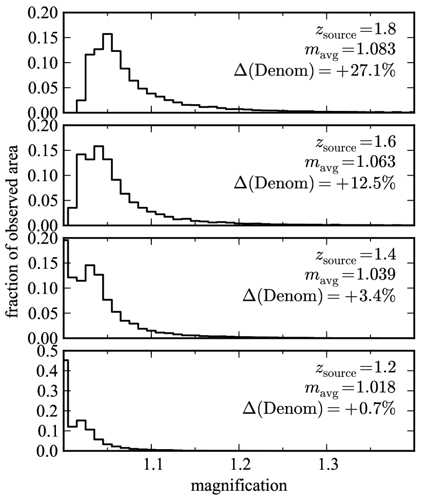
Figure 3.— Results of our lensing simulation: the magnification distribution in regions at radius $20^{\prime\prime}<r<100^{\prime\prime}$ in all 25 cluster fields (the approximate extent of the regions used in the rate analysis). The four panels correspond to source redshifts of $z_{s}=1.2,\ 1.4,\ 1.6,1.8$. For each source redshift, the average magnification $m_{\rm avg}$ is given. Under the approximation that all SNe are magnified by $m_{\rm avg}$, $\Delta({\rm Denom})$ shows the corresponding increase in the denominator of Equation (1). Note that this change in Denom considers only magnification; the effect of source-plane area shrinkage is considered separately in Figure 4. At $z<1.4$, where the survey’s sensitivity is greatest, magnification from lensing has only a $\lesssim 3\%$ effect on the detectability of SNe.

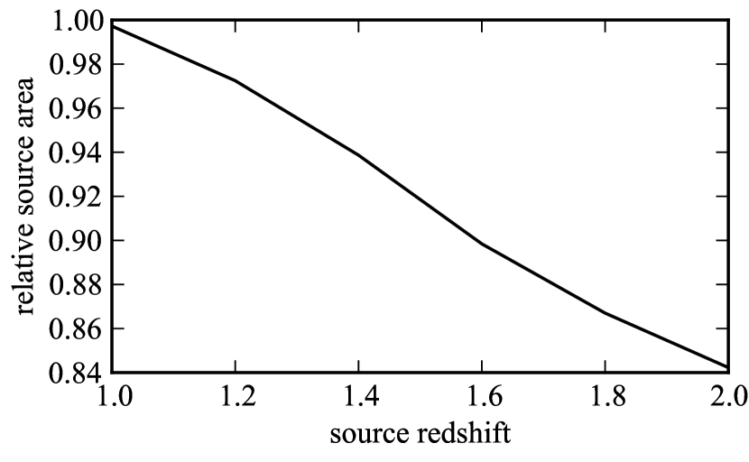
Figure 4.— True source-plane area relative to the observed area in our lensing simulation, as a function of source redshift. The relative area is for regions at radius $20^{\prime\prime}<r<100^{\prime\prime}$ in each of the 25 cluster fields (the approximate extent of the regions used in the analysis). The relative source area corresponds directly to the change in the denominator of Equation (1). The effect is opposite in sign to the effect in Figure 3.

We conclude from these simulations that the two effects cancel to within a few percent of the total rate, over the redshift range of interest: At $z=1.4$, magnification increases SN detectability by $\sim$3% and source-area reduction decreases detectability by $\sim$6%. At $z=1.6$, the increase is $\sim$12%, and the decrease is $\sim$10%. At $z=1.8$ the increase overwhelms the decrease ($\sim$27% versus $\sim$13%), but there will be very few SNe detected beyond $z\sim 1.6$ (see Figure 2). Therefore, we have not made an adjustment for these effects. Furthermore, the size of each effect is much smaller than other sources of systematic uncertainty considered below. For example, the average magnification at $z=1.8$ is only $\sim$1.08 ($-0.08$ mag), whereas below we consider the effect of changing the luminosity of all SNe in our simulation by $\pm 0.2$ magnitudes. So, we do not assign a specific systematic uncertainty to lensing effects.

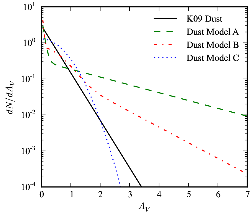
Figure 5.— Host galaxy dust extinction distributions, illustrating the behavior of the distributions at large $A_{V}$. The K09 distribution is used for our main result. Models A, B, and C are similar to the models of the same name examined in Dahlen et al. (2008) and are based on results from Hatano et al. (1998), Riello & Patat (2005) and Neill et al. (2006), respectively. These alternative distributions are used here to investigate possible systematic uncertainty due to host galaxy dust. This figure can be compared to Figure 3 of Dahlen et al. (2008).

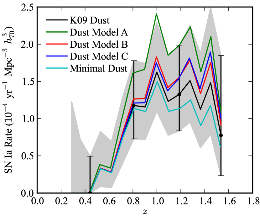
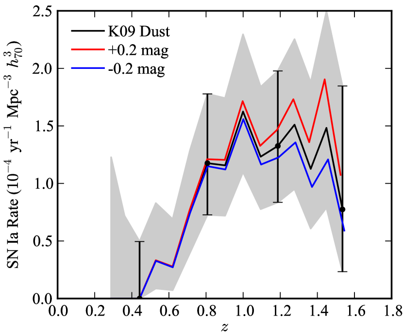
Figure 6.— The volumetric SN Ia rate in four redshift bins (points with error bars) of width $\Delta z=0.4$. The error bars represent the statistical-only uncertainty. The black line shows the rate calculated in a moving bin of width $\Delta z=0.4$ (shaded grey regions represent uncertainty). Note that the points with error bars are uncorrelated errors (using non-overlapping bins), while the uncertainty in the moving bin is correlated from point to point. Left Panel: The green, red, blue and cyan lines show the rate (with no uncertainty) assuming alternative SN color distributions. Right Panel: The red and blue lines show the rate assuming that all SNe are brighter or dimmer by $\pm 0.2$ mag.

4.3. Dust Extinction

The degree to which SNe are affected by host galaxy dust extinction is perhaps the largest systematic uncertainty in SN Ia rate studies. Here, we consider alternatives to the extinction distribution used in §3 and evaluate the effect on the results. Specifically, we reproduce three $P(A_{V})$ distributions considered in Dahlen et al. (2008) and Neill et al. (2006). In each of these models, as for our main result, we constrain $P(A_{V})=0$ for $A_{V}<0$.

The first, “Model A,” is used for the main result in Dahlen et al. (2008). It is based on the model of Hatano et al. (1998), constructed to estimate extinction in local disk galaxies. The distribution in Figure 3 of Dahlen et al. (2008) is well approximated by

$$P(A_{V})=0.61\frac{e^{-A_{V}/2}}{2}+0.39\frac{e^{-A_{V}/0.07}}{0.07}.$$ (5)

This distribution is shown in Figure 5. The second distribution we consider, “Model B,” is used by Dahlen et al. (2008) as an alternative distribution. It is based on the models in Riello & Patat (2005), which are aimed at generalizing the Hatano et al. (1998) models to a variety of dust properties and a variety of spiral Hubble types. Here we approximate the distribution by

$$P(A_{V}) = 0.35\delta(A_{V})+0.40\frac{2}{0.6\sqrt{2\pi}}e^{-A_{V}^{2}/(2\times 0.6^{2})}+$$ (6)

$$+~{}0.25e^{-A_{V}}.$$

where $\delta$ is the Dirac delta function, used here to assign 35% of SNe to the lowest host galaxy extinction bin. The third distribution we consider, labeled “Model C,” is used in the rate analysis of Neill et al. (2006). It is given by

$$P(A_{V})=\frac{2}{0.62\sqrt{2\pi}}e^{-A_{V}^{2}/(2\times 0.62^{2})}.$$ (7)

All three of these distributions are reproduced in Figure 5, and the corresponding distributions of SN color are shown in Figure 1 (right panel). In addition to these three distributions, we also consider a distribution with minimal dust, where we assume the SNLS $z<0.6$ sample is complete and fit it with a skewed Gaussian distribution. The effective visibility time for each dust model is shown in Figure 2 and the corresponding SN rate results are shown in Figure 6 (left panel).

Of all the models, Model A produces the most strikingly different results for the effective visibility time. Even in the lowest redshift bin ($0.2<z<0.6$) it implies that 10% of SNe are missed due to dust, relative to the K09 model. In the $0.6<z<1.0$ redshift bin, it yields effective visibility times lower by 27%, while Models B, C and the minimal dust model result in changes of only $-7\%$, $-3\%$, and $+3\%$ respectively. This is unsurprising: In Model A, 26% of SNe have host galaxy extinctions $A_{V}>2$ while this fraction is $<4\%$ in Model B and $<1\%$ in models K09 and C. In the $1.0<z<1.4$ bin Model A has the largest effect: $-33\%$ compared to the K09 model. As the work of Riello & Patat (2005, Model B) is aimed at generalizing Hatano et al. (1998, Model A) for use at higher redshifts, Model B may be viewed as more applicable. Along these lines, Cappellaro et al. (1999) have noted that using the Hatano et al. (1998) model appears to over-correct SN rates.

Still, for the systematic uncertainty associated with the choice of dust model we take a conservative approach, using the full range of these models. We use the minimal dust model to obtain the lower limit on the rate and Model A for the upper limit. This confidence range is shown in Table 3.

4.4. More Dust at High Redshift?

Several studies have pointed out that extinction is likely to increase with redshift, due to increasing star formation in dusty environments (Mannucci et al., 2007; Holwerda, 2008). The potential effect on the SN Ia extinction distribution is difficult to quantify as it depends not only on the relation between star formation and dust ejection but also the SN Ia delay time distribution. However, we estimate that any possible redshift-dependence is well-encompassed by the conservatively large range of extinction models we use above. Rowan-Robinson (2003) estimated that the average extinction $\langle A_{V}\rangle(z)$ peaks at $z\sim 1$, at a value $\sim$0.15 mag higher than locally. The effect of such an additional dimming on our rates at $z\sim 1$ is approximately 10%, whereas the extinction distribution uncertainty already included above is $\sim$50%. Similarly, Graur et al. (2011) estimated the fraction of missing SNe to be 5–13% in the redshift range $1<z<2$ based on the work of Mannucci et al. (2007). As the difference induced by our use of the K09 extinction model rather than model C used by Graur et al. is already much greater than this, we do not make an explicit correction for increasing dust at high redshift.

4.5. Other SN properties

In addition to the choice of the host galaxy dust extinction distribution, other assumptions about SN properties can affect the derived rates. These include the absolute magnitude, the stretch distribution, and the spectral time series template. Fortunately these properties are well constrained. For example, shifting the stretch distribution by $\Delta s=\pm 0.05$ would be inconsistent with the observed distribution, and similarly for the color distribution. The average absolute magnitude of SNe Ia (in our cosmology) is constrained to much better than $0.1$ mag (Amanullah et al., 2010). To first order, changing any of these assumptions affects the derived rate by increasing or decreasing the luminosity of the simulated SN and thereby increasing or decreasing the effective visibility time. Therefore, to estimate the effect of such changes on the result, we simply shift the absolute magnitude of the simulated SNe Ia. A shift in stretch of $\Delta s=\pm 0.05$ is equivalent to a magnitude shift of $\Delta M_{B}=\alpha\Delta s=0.08$. Similarly, a shift in color of $\Delta c=\pm 0.05$ is equivalent to a magnitude shift of $\Delta M_{B}=\beta\Delta c=0.11$. Conservatively then, we use a $\pm 0.2$ mag shift to jointly capture these uncertainties and uncertainty in the absolute magnitude. The effect on the results is shown in Figure 6 (right panel) and is generally comparable to or smaller than the effect from the extinction distribution uncertainty (see Table 3).

4.6. Cosmic Variance and galaxy-cluster correlation

There are various effects that could increase or decrease the density of galaxies in the observed fields relative to the cosmic average, potentially biasing the volumetric rates. We have estimated all such effects to be small ($\lesssim 5\%$). We briefly discuss three of these effects.

(1) Masking volume surrounding clusters. Any SN occurring in the volume around a cluster (within $|\Delta z|\lesssim 0.015$) but not associated with the cluster would be mistakenly assigned to the cluster. This volume is therefore effectively not counted for this analysis. We estimate that this decreases the total volume in the $0.6<z<1.0$ redshift bin by $\approx$1.5% (due to the presence of 5 clusters) and in the $1.0<z<1.4$ bin by $\approx$6% (due to the presence of 20 clusters). Because the next effect compensates somewhat for this effect, we do not make an explicit correction in the result.

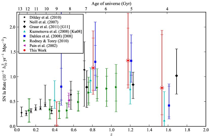
Figure 7.— Volumetric SN Ia rates from the HST Cluster Supernova Survey (red points) compared to key rates from the literature. For measurements with two error bars, including ours, the inner and outer error bars represent the statistical (Poisson) and total (statistical + systematic) uncertainties, respectively. Measurements with a single error bar (Ku08 and G11) are Bayesian-based analyses where the error bar encompasses both statistical and typing uncertainties. Some measurements have been offset slightly in redshift for visibility. Note that we have conservatively reported our measurement in the highest-redshift bin as having a lower limit of zero due to redshift uncertainty in the single SN in this bin.

(2) Cluster-galaxy correlation. There may be an increase in the density of field galaxies (relative to the cosmic average) in the volume surrounding the cluster due to the presence of the cluster itself. However, we estimate that this effect should be small outside of the volume discussed in the previous effect. At $z=1$, a redshift difference of $\Delta z=0.015$ corresponds to a comoving distance of $\sim$36 Mpc. Density fluctuations on these scales are in the linear regime. At 36 Mpc, the correlation function of massive galaxies is $\xi\lesssim 0.2$ (e.g., Eisenstein et al., 2005; White et al., 2011). Even if the average over-density at scales 36 Mpc $<r<$ 100 Mpc were 0.2 (an overestimate), this would only be a 2–3% effect on the total galaxy density in a bin of width $\Delta z=0.4$.

(3) Cosmic variance. Cosmic variance could affect the results if there is an under-density or over-density of field galaxies in the observed regions (relative to the cosmic average). In B11, we estimated the size of this effect in the GOODS fields, finding it to contribute a systematic uncertainty of 4–6% based on the cosmic variance calculator of Trenti & Stiavelli (2008) and the difference between the GOODS-N and GOODS-S fields (see also discussion in Dahlen et al., 2008). The effect is even smaller for the 25 fields in this study: here we have more than two widely separated fields, providing a better sampling of cosmic variance.

5. Discussion

The results from this study are available as a machine-readable table from the Journal or the survey website. We include the product of the effective visibility time and observed area, as a function of redshift (Figure 2), for a variety of assumptions about SN properties and host galaxy dust distributions. With these data and the SN candidate list, the rates from this survey can be recomputed in any arbitrary redshift bin and for any of these assumptions. This will make it easy to combine these results with other measurements for increased statistical power.

5.1. Comparison to Other High-Redshift Measurements

In Figure 7 we compare our results to an assortment of other volumetric SN Ia rate measurements. (All measurements have been corrected to our assumed cosmology.) Our results are generally consistent with the three published measurements at $z\gtrsim 1$: Kuznetsova et al. (2008, hereafter Ku08), Dahlen et al. (2008, hereafter D08), and Graur et al. (2011, hereafter G11). D08 and G11 supplant earlier results from Dahlen et al. (2004) and Poznanski et al. (2007), respectively. The Ku08 and D08 measurements are based on SN searches in the HST GOODS fields, with Ku08 being an independent analysis of a subset of the data used in D08. These SN searches used ACS to cover the GOODS fields with a 45 day cadence and triggered followup (imaging and spectroscopy) of SN candidates. The D08 analysis uses a SN typing method based on both spectroscopy and photometry (similar to the approach used here) while Ku08 use a photometric-only pseudo-Bayesian approach to typing. The G11 measurement is based on “single-detection” searches in the Subaru Deep Field. G11 also use a pseudo-Bayesian typing approach, but use a single detection with observations in three filters, rather than multiple detections with observation in (typically) two filters as in Ku08.

Table 4Rate Comparison Using Consistent Extinction Distributions

	$0.6<z<1.0$	$1.0<z<1.4$	$1.4<z<1.8$
This work using extinction model A	$1.61^{+0.83}_{-0.62}$	$1.99^{+0.98}_{-0.74}$	$1.08^{+1.50}_{-0.76}$
D08	$1.30^{+0.33}_{-0.27}$	$1.32^{+0.36}_{-0.29}$	$0.42^{+0.39}_{-0.23}$
This work using minimal extinction model	$1.14^{+0.58}_{-0.43}$	$1.14^{+0.56}_{-0.42}$	$0.62^{+0.86}_{-0.44}$
Ku08	$0.93^{+0.25}_{-0.25}$	$0.75^{+0.35}_{-0.30}$	$0.12^{+0.58}_{-0.12}$
	$0.5<z<1.0$	$1.0<z<1.5$	$1.5<z<2.0$
This work using extinction model C and +5 – 13% high-$z$ correction	$1.01^{+0.52}_{-0.39}$	$1.69^{+0.75}_{-0.58}$	$0.00^{+1.92}_{-0.00}$
G11	$0.79^{+0.33}_{-0.41}$	$0.84^{+0.25}_{-0.28}$	$1.02^{+0.54}_{-0.37}$

Note. — Rate in units of $10^{-4}$ $h_{70}^{3}$ yr^-1 Mpc^-3. Confidence intervals are statistical (Poisson).

5.2. The Effect of Different Extinction Distributions

Although our results generally agree with all three previous studies (Ku08, D08, G11), it is interesting to compare in more detail the assumptions used in each study. Here we focus specifically on differences in the assumed extinction distribution, which we find to be the dominant systematic. Unlike systematic uncertainties arising from SN typing, systematic uncertainty due to assumptions about SN properties will be common between rate studies, potentially leading to a systematic offset between results if different assumptions are used in different studies.

For example, our results appear very similar to D08 in the two mid-redshift bins (within 10% in both bins). However, D08 assume a different extinction distribution in their simulations than we do. If we assume the same distribution (extinction model A), our derived rates in these two bins are 1.61 and 1.99 $\times 10^{-4}$ $h_{70}^{3}$, compared to 1.30 and 1.32 $\times 10^{-4}$ $h_{70}^{3}$ in D08. (Conversely, if D08 had used the K09 extinction model, their rates would have been lower than ours.) In other words, we actually found more SNe Ia than one would have predicted based on D08 (but not inconsistently so given the large Poisson uncertainties).

Note that D08 also compare Models A, B and C in assessing their systematic uncertainty but do not find the large differences that we find here. They find that Model B produces rates that are $\lesssim 10\%$ lower than Model A (only $\sim$$4\%$ in the highest redshift bin), and that Model C has even less of an effect, whereas we find that the difference beyond Models A and B is approximately 26% in the central two bins. These different findings regarding the systematic uncertainty due to extinction are surprising given that both studies are based on HST searches the same band to similar depths. One possible explanation is the difference in cadence ($\sim$23 days here versus $\sim$45 days in GOODS). We checked the impact of a longer cadence by rerunning our simulations ignoring every other epoch in our search. We find that the effect of different extinction distributions is unchanged to within a few percent. That is, the shorter $\sim$23 day cadence is not significantly more sensitive to highly reddened SNe than the $\sim$45 day cadence. The slight enhancement in reach that a short cadence affords is insignificant compared to the long $A_{V}$ tail of, for example, Model A. It is possible that the difference in estimated systematic uncertainty could arise from some other detail of the efficiency simulations, but a full resimulation of the D08 efficiency calculations is beyond the scope of this paper.

In Table 4 we have recomputed our rates using extinction assumptions similar to D08, Ku08 and G11. Ku08 use only two discrete values for $A_{V}$. The values, 0.0 and 0.4, are relatively small, so we compare using our “minimal dust” model. G11 use the distribution of N06 (Model C) with a $+$5–13% correction in the redshift range $1.0<z<2.0$ as discussed earlier (§4.4). Table 4 serves two purposes: (1) it aids direct comparison between each of these studies and our result, and (2) it illustrates how much the assumed extinction distribution affects our result.

In light of the large systematic differences due to dust, it is vitally important to use caution when comparing rate results from studies that use different dust assumptions. In particular, systematic offsets from dust assumptions could affect the shape of the derived SN Ia delay time distribution. The DTD shape is obtained not from the SN rate itself, but from the change in the rate with redshift (see, for example, Figure 2 of Horiuchi & Beacom, 2010). To measure the change, one typically must compare surveys covering different redshift ranges. Comparing low- and high-redshift measurements that correct their rates using different extinction distributions will induce a systematic error on the slope of the SN rate and thereby the DTD shape.

To avoid such a systematic bias, studies of the DTD should strive to use consistent extinction corrections between low and high redshift. To aid this, we have provided our rates calculated under a variety of extinction assumptions. Consitency will go a long way towards reducing potential errors in the DTD, even if the extinction distribution remains poorly known. However, in the long run one would like a better understanding of SN extinction distributions at both low and high redshift, particularly to avoid uncertainties due to a changing extinction distribution with redshift. The prospects for directly detecting the highly extincted SNe are not great: even with a deep IR search, most SNe with $A_{V}>2$ will be missed at high redshift. The alternative is more precise updated modeling of SN Ia extinction in the vein of Riello & Patat (2005) or Mannucci et al. (2007) that takes into account factors such as the evolution of extinction with delay time and our latest knowledge of the SN Ia DTD.

5.3. Summary

In this paper we have computed volumetric SN Ia rates based on 189 HST orbits. This large HST dataset adds statistics to the existing HST rate measurements, previously based only on the GOODS fields. Our results provide additional strong evidence that the SN Ia rate is $\gtrsim 0.6\times 10^{-4}$ $h_{70}^{3}$ yr^-1 Mpc^-3 at $z\sim 1$. The availability of raw data from our efficiency simulations makes it simple to combine this dataset with current and future HST datasets, such as the 902-orbit Cosmic Assembly Near-IR Deep Extragalactic Legacy Survey (CANDELS; Grogin et al., 2011), for even greater statistical gains.

We find that an important systematic uncertainty in our result is the amount of host-galaxy dust assumed in our simulations. This illustrates the need to use caution in comparing SN rate results from different surveys, especially as statistical uncertainty decreases and systematic uncertainties become dominant. Consistent comparisons and updated extinction models can drastically reduce the dust systematic in future studies.

References

- Amanullah et al. (2010) Amanullah, R., et al. 2010, ApJ, 716, 712
- Astier et al. (2006) Astier, P., et al. 2006, A&A, 447, 31
- Barbary et al. (2011) Barbary, K., et al. 2011, preprint (arXiv:1010.5786)
- Barbary et al. (2009) Barbary, K., et al. 2009, ApJ, 690, 1358
- Brodwin et al. (2011) Brodwin, M., et al. 2011, ApJ, 732, 33
- Cappellaro et al. (1999) Cappellaro, E., Evans, R., & Turatto, M. 1999, A&A, 351, 459
- Chotard et al. (2011) Chotard, N., et al. 2011, A&A, 529, L4
- Dahlen et al. (2008) Dahlen, T., Strolger, L.-G., & Riess, A. G. 2008, ApJ, 681, 462
- Dahlen et al. (2004) Dahlen, T., et al. 2004, ApJ, 613, 189
- Dawson et al. (2009) Dawson, K. S., et al. 2009, AJ, 138, 1271
- Dekel & Silk (1986) Dekel, A. & Silk, J. 1986, ApJ, 303, 39
- Dilday et al. (2010) Dilday, B., et al. 2010, ApJ, 713, 1026
- Eisenhardt et al. (2008) Eisenhardt, P. R. M., et al. 2008, ApJ, 684, 905
- Eisenstein et al. (2005) Eisenstein, D. J., et al. 2005, ApJ, 633, 560
- Giavalisco et al. (2004) Giavalisco, M., et al. 2004, ApJ, 600, L93
- Goobar et al. (2009) Goobar, A., et al. 2009, A&A, 507, 71
- Graur et al. (2011) Graur, O., et al. 2011, MNRAS, 417, 916
- Grogin et al. (2011) Grogin, N. A., et al. 2011, preprint (arXiv:1105.3753)
- Guy et al. (2010) Guy, J., et al. 2010, A&A, 523, A7
- Hatano et al. (1998) Hatano, K., Branch, D., & Deaton, J. 1998, ApJ, 502, 177
- Hicken et al. (2009) Hicken, M., Wood-Vasey, W. M., Blondin, S., Challis, P., Jha, S., Kelly, P. L., Rest, A., & Kirshner, R. P. 2009, ApJ, 700, 1097
- Hilton et al. (2007) Hilton, M., et al. 2007, ApJ, 670, 1000
- Hilton et al. (2009) Hilton, M., et al. 2009, ApJ, 697, 436
- Holwerda (2008) Holwerda, B. W. 2008, MNRAS, 386, 475
- Horiuchi & Beacom (2010) Horiuchi, S. & Beacom, J. F. 2010, ApJ, 723, 329
- Hsiao et al. (2007) Hsiao, E. Y., Conley, A., Howell, D. A., Sullivan, M., Pritchet, C. J., Carlberg, R. G., Nugent, P. E., & Phillips, M. M. 2007, ApJ, 663, 1187
- Hsiao et al. (2011) Hsiao, E. Y., et al. 2011, in STScI 2010 Calibration Workshop, ed. S. Deustua and C. Oliveira (in press)
- Huang et al. (2009) Huang, X., et al. 2009, ApJ, 707, L12
- Iben & Tutukov (1984) Iben, Jr., I. & Tutukov, A. V. 1984, ApJS, 54, 335
- Jee et al. (2011) Jee, M. J., et al. 2011, ApJ, 737, 59
- Jee et al. (2009) Jee, M. J., et al. 2009, ApJ, 704, 672
- Kessler et al. (2009) Kessler, R., et al. 2009, ApJS, 185, 32
- Kowalski et al. (2008) Kowalski, M., et al. 2008, ApJ, 686, 749
- Kuznetsova et al. (2008) Kuznetsova, N., et al. 2008, ApJ, 673, 981
- Li et al. (2011) Li, W., et al. 2011, MNRAS, 412, 1441
- Livio (2001) Livio, M. 2001, in Supernovae and Gamma-Ray Bursts: the Greatest Explosions since the Big Bang, ed. M. Livio, N. Panagia, & K. Sahu, 334–355
- Mannucci et al. (2007) Mannucci, F., Della Valle, M., & Panagia, N. 2007, MNRAS, 377, 1229
- Matteucci & Greggio (1986) Matteucci, F. & Greggio, L. 1986, A&A, 154, 279
- Melbourne et al. (2007) Melbourne, J., et al. 2007, AJ, 133, 2709
- Meyers et al. (2011) Meyers, J., et al. 2011, ApJ, submitted
- Morokuma et al. (2010) Morokuma, T., et al. 2010, PASJ, 62, 19
- Navarro et al. (1997) Navarro, J. F., Frenk, C. S., & White, S. D. M. 1997, ApJ, 490, 493
- Neill et al. (2007) Neill, J. D., et al. 2007, in American Institute of Physics Conference Series, Vol. 924, The Multicolored Landscape of Compact Objects and Their Explosive Origins, ed. T. di Salvo, G. L. Israel, L. Piersant, L. Burderi, G. Matt, A. Tornambe, & M. T. Menna, 421–424
- Neill et al. (2006) Neill, J. D., et al. 2006, AJ, 132, 1126
- Pain et al. (2002) Pain, R., et al. 2002, ApJ, 577, 120
- Poznanski et al. (2007) Poznanski, D., et al. 2007, MNRAS, 382, 1169
- Riello & Patat (2005) Riello, M. & Patat, F. 2005, MNRAS, 362, 671
- Ripoche et al. (2011) Ripoche, P., et al. 2011, ApJ, submitted
- Rodney & Tonry (2010) Rodney, S. A. & Tonry, J. L. 2010, ApJ, 723, 47
- Rosati et al. (2009) Rosati, P., et al. 2009, A&A, 508, 583
- Rowan-Robinson (2003) Rowan-Robinson, M. 2003, MNRAS, 345, 819
- Santos et al. (2009) Santos, J. S., et al. 2009, A&A, 501, 49
- Scannapieco et al. (2006) Scannapieco, C., Tissera, P. B., White, S. D. M., & Springel, V. 2006, MNRAS, 371, 1125
- Sharon et al. (2010) Sharon, K., et al. 2010, ApJ, 718, 876
- Strazzullo et al. (2010) Strazzullo, V., et al. 2010, A&A, 524, A17
- Strolger et al. (2010) Strolger, L., Dahlen, T., & Riess, A. G. 2010, ApJ, 713, 32
- Sullivan et al. (2000) Sullivan, M., Ellis, R., Nugent, P., Smail, I., & Madau, P. 2000, MNRAS, 319, 549
- Sullivan et al. (2011) Sullivan, M., et al. 2011, ApJ, 737, 102
- Suzuki et al. (2011) Suzuki, N., et al. 2011, preprint (arXiv:1105.3470)
- Thielemann et al. (1996) Thielemann, F., Nomoto, K., & Hashimoto, M. 1996, ApJ, 460, 408
- Trenti & Stiavelli (2008) Trenti, M. & Stiavelli, M. 2008, ApJ, 676, 767
- Tsujimoto et al. (1995) Tsujimoto, T., Nomoto, K., Yoshii, Y., Hashimoto, M., Yanagida, S., & Thielemann, F. 1995, MNRAS, 277, 945
- Webbink (1984) Webbink, R. F. 1984, ApJ, 277, 355
- Whelan & Iben (1973) Whelan, J. & Iben, I. J. 1973, ApJ, 186, 1007
- White et al. (2011) White, M., et al. 2011, ApJ, 728, 126
- Yungelson & Livio (2000) Yungelson, L. R. & Livio, M. 2000, ApJ, 528, 108