From the cosmological model to generation of
the Hubble flow

Abstract

We review different approaches to the problem of generating the observed Hubble flow, whose discussion was pioneered by A.D. Sakharov. Extrapolating the Cosmological Standard Model to the past makes it possible to determine physical properties of and conditions in the early universe. We discuss a new cosmogenesis paradigm based on studying geodesically complete geometries of black/white holes with integrable singularities.

1 Introduction

In his works (e.g. [1, 2]) A.D. Sakharov repeatedly mentioned the idea that cosmological flows can be generated from ultra-high density states of matter through quantum transitions resulting in different values of the world constants, signature, time arrow and other geometrical features of space–time. The way how gravitational systems and parts thereof enter and leave such critical states remains a point of controversy up till now.

High curvature and density are naturally generated in separate spacetime domains in the course of collapse of compact astrophysical objects that end up as black holes. However, the problem of how collapse turns into expansion is yet to be solved. The paradigm of multi-sheet universe proposed by A.D. Sakharov as well as the widely accepted Multiverse paradigm (see, for example, [3]) requires a clear and straightforward physical mechanism of generating multiple expanding matter flows. Still, the mechanism of cosmogenesis is rather vague. In order to study it we need to know the structure of the initial material flow called the early universe with sufficient precision.

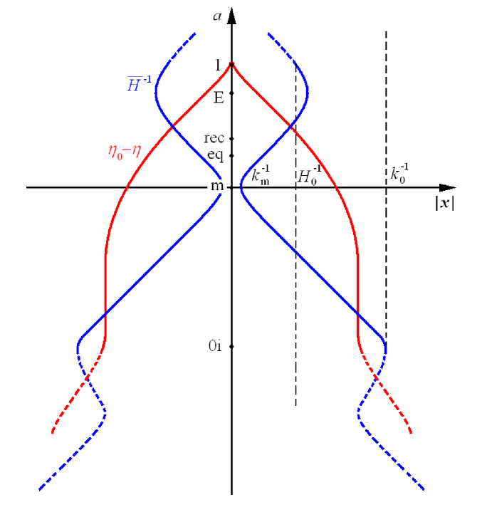
Figure 1: Vertical axis shows the scale factor $a$ while the horizontal one – the comoving coordinate $|\mathbf{x}|$ (an observer’s world line is $\mathbf{x}=0$). The line $\overline{H}^{\,-1}$ corresponds to the Hubble radius($\overline{H}=aH$), and $(\eta_{0}-\eta)$ is the light cone of the past. The scales $k_{\rm{m}}^{-1}$, $H_{0}^{-1}$, and $k_{0}^{-1}$, correspond to submillimeters, 4.3 Gpc, and the size of the Friedmannian world, respectively. The moments of time $\rm m$, $\rm eq$, $\rm E$, and $\rm rec$, mark the end of the inflationary Big Bang stage, the onsets of DM and DE eras, and recombination, respectively.

The problem of determining geometrical properties of the early universe was successfully solved at the turn of the 21st century in the Cosmological Standard Model (CSM) which describes the entire set of experimental and observational data in the energy range $10^{-3}-10^{12}$ eV. The CSM made it possible to restore the initial state of the universe by a direct extrapolation to the past with a mere assumption that General Relativity (GR) holds up to the GUT scale ($\sim 10^{25}$ eV). Further extrapolation to higher energies is rather problematic because of the inflationary Big Bang stage. At the latter stage the Hubble radius outgrows the light horizon of the past where most information about pre-inflationary geometry of the flow is stored (see Fig. 1, [4]). Going to the past deviations from the quasi-Friedmannian model increase during inflation. Hence, the cosmological flow structure at the onset of inflation could be well too different from the Friedmannian one and have a different symmetry and topology.

By virtue of the CSM the problem of generating the initial expanding flow (the cosmogenesis problem) has come into strict scientific domain, because energies do not cross the Planck scale. Besides, since ultra-high energies and curvature occur in the gravitating system during only a short period of time, in studying models with collapse turning into expansion it is sufficient to use only local conservation laws which may be written in the general geometric form of the Bianchi identities. To do so, any modification of gravity or quantum-gravitational corrections are included in the right-hand side and ascribed to an effective energy–momentum tensor, thus, containing both material and, in part, spacetime degrees of freedom. This approach allows us to keep the notion of mean metric space–time (regardless of density and curvature values) and stay in the class of geometries with integrable singularities, which makes it possible to construct geodesically complete maps of black/white holes and understand how the $T$-region of a black hole is gravitationally transformed into anticollapse of a newly generated matter in the white hole (cosmological expansion).

We review below lessons taught by the extrapolation, determine initial conditions in the early universe, discuss the physical nature of the multi-sheet universe and present new models of cosmological flow generation in the framework of the cosmogenesis paradigm we have proposed (see [5]).

2 Lessons of extrapolation

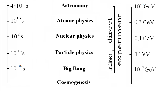
Figure 2: Experimental basis of the early universe. The curvature radius (in seconds) of the universe is on the left vertical axis, characteristic energies are on the right axis.

The cornerstone of the CSM is a vast observational and experimental basis spanning 15 orders of magnitude in energy: from the current cosmological density ($\sim 10^{-3}$ eV) to the electroweak scale ($\sim 10^{12}$ eV) studied at the Large Hadron Collider and corresponding to the age of the universe of a few picoseconds (see Fig. 2). In the present time this is established scientific knowledge rather than extrapolation. The extrapolation begins at higher energies and spans another 13 orders of magnitude up to the GUT scale.

The most important result of the contemporary research is our knowledge of the geometry of the early universe, which is equivalent to the structure of metric and energy–momentum tensors in GR. The empirically developed model has a small parameter – the amplitude of cosmological metric inhomogeneities ($\sim 10^{-5}$), which allows us to exploit perturbation theory techniques. In the zeroth order we deal with the spatially flat Friedmann model described by a single function of time – the scale factor $a(t)$ defined by matter contents. In the first order the tensors’ structure is more complicated and expressed through three irreducible forms [6]: scalar (density perturbations), tensor (gravitational waves) and vector (related to magnetic fields, for example) ones. Each of them is characterized by its power spectrum, $S(k)$, $T(k)$ and $V(k)$, where $k$ is the wave number (inverse scale of perturbation). With spatial phase being random, the second order and higher ones do not contain new free functions.

Therefore, we conclude that the initial cosmological matter flow is fully deterministic and possesses a laminar quasi-Hubble structure (weakly inhomogeneous, or quasi-Friedmannian universe). Provided that the initial conditions and matter contents are set, the world develops into the rich palette of physical processes and phenomena we currently observe. At the moment we know two first functions of the four mentioned above in the range available to observational cosmology. If the up-and-running PLANCK experiment succeeds the power spectrum of gravitational waves will be revealed as well. Detection of the vector mode is beyond our experimental capability so far.

The main goal of the cosmogenesis problem is to explain the starting properties of the cosmological flow. Its physical formulation stems from the lessons of extrapolation in the past [4]. Seven of them we review below.

1) The universe is large. This fact can be explained by the short-period inflationary Big Bang stage that precedes the radiation-dominated expansion era.

The current Hubble radius (4-curvature radius) is $H^{-1}_{0}\simeq 4.3$ Gpc, which, on the time scale, lies 60 orders of magnitude away from the Planck value. According to the CSM, during this period the scale factor could grow mere 30 orders as confirmed by the Friedmann equations describing the main order of perturbation theory:

$$H\equiv\frac{\dot{a}}{a}=H_{0}\sqrt{\frac{10^{-4}}{a^{4}}+\frac{0.3}{a^{3}}+0.7}\;\;\rightarrow\;\frac{H_{0}}{100a^{2}}\,,$$ (1)

$$\gamma\equiv-\frac{\dot{H}}{H^{2}}=\frac{2\cdot 10^{-4}+0.4\cdot a}{10^{-4}+0.3\cdot a+0.7\cdot a^{4}}\;\in\;\left(0.4\,,\,2\right)$$

(three terms under the square root correspond to radiation, non-relativistic matter and dark energy; the scale factor is measured in units of its modern value). Extrapolating to the past we obtain the universe dominated by radiation. Its size at early times is at submillimeter scale, which is extremely big being 30 orders of magnitude greater than the Planck scale. In order to explain this size one needs to introduce a preceding inflationary stage with $\gamma<1$ and no less than 70 Hubble epochs ($\sim 30\ln 10$).

2) Causality principle is independent evidence of the inflationary Big Bang stage.

As follows from eqs. (1), in the radiation-dominated era galactic scales appear to reside in causally disconnected zone (see Fig. 1). They could enter this zone from a causally connected region if there had existed a short inflationary stage.

3) Small tensor mode (indicating the inflationary Big Bang as well) and a Gaussian field of density perturbations.

While the zeroth order of perturbation theory is described by the Friedmann equations the first order consists of oscillators (see Appendix). The modes $S$ and $T$ evolve as massless scalar fields $q=(q_{S},q_{T})$ under the action of the external gravitational field of the non-stationary Hubble flow, which leads to parametric amplification of the $q$ fields in the course of cosmological expansion [7, 4]. Under quite general assumptions on the expansion rate the equations governing the behavior of the elementary oscillators yield a general solution with excitation amplitudes depending on initial conditions. For oscillators initially occupying the ground state the power spectra of the generated perturbations are the following:

$$T(k)\simeq\frac{H^{2}}{M_{P}^{2}}\;<\;10^{13}\;\mbox{GeV}\;,\qquad\frac{T}{S}\simeq 4\gamma\;<\;0.1\;,$$ (2)

where $\langle q^{2}_{S,T}\rangle=\int(S,T)\frac{dk}{k}$ . The brackets $\langle\ldots\rangle$ stand for averaging over the state, $M_{P}\equiv G^{-1/2}\simeq 10^{19}$ GeV – the Planck mass. As one can see the theory does not discriminate between the tensor and scalar modes while their ratio depends on the value $\gamma$ in the parametric amplification era. Non-equalities in (2) reflect current observational bounds on cosmological gravitational waves. The second inequality indicates that $\gamma$ in the early universe was less than one, which is indirect evidence of the inflationary start of the Hubble flow. Hard evidence of primordial inflation will become available after the tensor mode is detected in observations of cosmic microwave background and the predicted relation between the $T$-spectrum index and the tensor-scalar amplitude ratio is confirmed ($n_{T}\equiv d\ln T/d\ln k\simeq-2\gamma\simeq-0.5\cdot T/S$).

It is worth pointing out that the latter conclusion is based on the hypothesis that the early Hubble flow was ideal, which implies the vacuum initial condition for $q$-fields. The assumption is justified by the fact that, first, the observed random spatial distribution of large-scale density perturbations is Gaussian (a property of quantum fluctuations linearly transferred to the field of inhomogeneities) and, second, the time phase of acoustic oscillations corresponds to the growing adiabatic evolution mode (a property of the parametric amplification effect).

4) Dark matter presence.

Nonlinear halos hosting galaxies consist of non-relativistic particles of dark matter (DM) that neither interact with baryons nor with radiation. The nature of DM particles is unknown, but there are observational indications that the origin of DM is related to the baryon asymmetry of the universe. Here are two of them: cosmological mass densities of DM and baryons are close to each other (the ratio is 5) and scales of their spatial large-scale distributions coincide (the cosmological horizon at the moment of equal densities of relativistic and non-relativistic components is identical to the sound horizon at the era of hydrogen recombination). If we take into account that the density ratio for the two non-relativistic components does not change with time we have to conclude that the reasons that led to generation of DM and to baryon asymmetry are interconnected. Both DM particles and extra baryons may have emerged in non-equilibrium processes of particle transformation in high-temperature radiation plasma of the Hubble flow. If this is the case, their origin has nothing to do with pre-inflationary history of the Big Bang.

5) Evidence of dark energy.

The matter forming the structure of the universe is tracked by gravitational potential gradient in dynamical observations of galaxies and gas and by gravitational lensing. Its amount does not exceed $30\%$ of the critical density. The rest $70\%$ reside in homogeneously distributed medium that does not interact with light and baryons. This is the so-called dark energy (DE) with negative effective pressure whose absolute value is comparable to the DE density. We have probably encountered a relic ultra-weak field which had remained “frozen” at the radiation- and matter-dominated eras and then started slowly rolling under the action of its own gravity 3.5 billion years ago. If it is true we are witnessing relaxation of the massive field, which opens a new look on the history of the Hubble flow.

6) History of the universe evolution.

One can see that the history of evolution includes periods of accelerated ($\gamma<1$) as well as decelerated ($\gamma>1$) expansion. The former include inflationary stages of the Big Bang and DE and the latter – the radiation- and matter-dominated eras. We know, however, that small perturbations decay if $\gamma<1$ and grow otherwise. Thus, it happens that in the history of the universe there were stages of forming (restoring) and decaying Hubble flow (in the latter case the structure is formed). This feature reveals a dual nature of long-range gravity capable of creating highly ordered configurations from quite general initial distributions and types of matter. Those are anticollapse, or inflation (formation of the ideal Hubble flow) and its antipode collapse (formation of gravitationally bounded halos and black holes). Therefore, we can look on the dynamical history of the flow as a 14-billion history of massive scalar fields relaxing to their minimal-energy states. Here comes the seventh and last lesson of extrapolation of the CSM to the pre-inflationary universe. How can the conditions necessary for the expanding matter flow to emerge and inflate into the observed Hubble flow, be created?

3 Cosmogenesis conditions

As a matter of fact, any solution of the cosmogenesis problem must answer three questions:

• How do the high densities emerge?

• What triggers the expansion?

• What is the origin of the cosmological symmetry?

Inflation does not address these questions. In its different models (e.g. [8, 9]) new physical fields are introduced in an ultra-dense state from the very beginning. The birth of the universe from “nothing” [10, 11] also involves the notion of a highly dense “false” vacuum, so do models with modified gravity [12]. It is true that in the so-called bouncing models, which have been developed for more than 40 years, the problem of initial conditions does not arise at all (thanks to modifications of equation-of-state), but again the Friedmannian symmetry is postulated.

The fundamental scientific principle that states that any physical solution describing nature must contain only such observable quantities that remain finite, appears to be of great use in the cosmogenesis problem. Indeed, if we consider realistic models of black/white holes with smoothed metric singularities this allows us to constrain the tidal forces (despite a possible divergence of some curvature components) and construct a geodesically complete metric space–time on the basis of dynamical solutions resulting from the energy–momentum conservation [5]. Here the singularity emerging around the collapsed object is surrounded by an effective matter. We model the latter in a wide class of equations-of-state. Now the radial geodesics pass to the $T$-region of the white hole rather than end in the singularity. From this point we arrive to a hypothesis that any black hole that has originated from the collapse of an astrophysical object may give birth to a new (daughter, or astrogenic) universe.

This conjecture easily solves all of the three above-mentioned problems of cosmogenesis:

• The ultra-high curvature and density on the initial stage of cosmological evolution are achieved as a consequence of superstrong and highly variable gravitational fields that exist inside the black/white hole and generate a matter the daughter universe consists of.

• The initial push to the expansion of the generated matter (the Big Bang) is provided by the $T$-region of the white hole. The initial cosmological impetus is, hence, of pure gravitational nature and one of the manifestations of gravitational (tidal) instability.

• The $T$-region symmetry of the black hole outside the maternal matter of the collapsing object is that of an anisotropic cosmology. It is transferred to the white-hole $T$-region and can be made isotropic by the known inflationary mechanisms.

4 Black/white holes with integrable singularity

The above-mentioned principle applied to spherically symmetric metrics of general type practically implies finiteness of the real functions $N$ and $\Phi$  in  $\mathbb{R}^{2}\in(r,t)$:

$$ds^{2}=N^{2}(1+2\Phi)\,dt^{\,2}-\frac{dr^{\,2}}{1+2\Phi}-r^{2}d\Omega\,,$$ (3)

where $r$ and $t$ are, respectively, radial and time coordinate in $R$-regions of the space-time ($\Phi>-1/2$) and, vice versa, time and radial coordinate of the same solution in $T$-regions ($\Phi<-1/2$, see [13]) while $d\Omega$ is the squared line element on the surface of 2-dimensional sphere.

The GR equations yield:

$$\Phi=-\frac{Gm}{r}\,,$$ (4)

where the finite mass function

$$m=m\!\left(r,t\right)=4\pi\!\int_{0}T_{t}^{t}r^{2}dr$$ (5)

vanishes on the inversion line $r=0$ thanks to the finiteness condition applied on the potential $\Phi$. $T_{t}^{t}$ is the $tt$-component of the energy–momentum tensor which can be written as $T_{\mu}^{\nu}=diag(-p,\,\varepsilon,-p_{\perp},-p_{\perp})$, provided spatial flows in the $T$-region are absent. Integrability of the function $T_{t}^{t}r^{2}$ at zero (which also follows from the finiteness condition) leads us to the definition of integrable singularity $r=0$ surrounded by an effective matter. We give below two examples of the models in which energy density is generated through variations of the transversal pressure $p_{\perp}$ changing in a triggered way at certain moments of time $r$. These models have finite tidal forces along the radial geodesics, and world lines of test particles are continued from the $T$-region of the black hole to that of the white hole. In other words, the tidal gravitational interaction in the vicinity of the integrable singularity undergoes an oscillation in time which connects the interiors of both holes. This phenomenon can be referred to as a collapse inversion.

5 Astrogenic universes

The matter in the $T$-regions of the vacuum solutions can be generated through time variations of the function $p_{\perp}(r)$, e.g. through discontinuities of first kind, since equations-of-motion do not contain its derivatives (energy density is pumped from the gravitational field and the metrics is consistently reconfigured to satisfy GR). For simplicity the longitudinal pressure is conveniently chosen to be vacuum-like ($p=-\varepsilon$). Hence, $N=1$ everywhere in $\mathbb{R}^{2}$ and the matter is at rest in the reference frame (3), the energy density being found from the Bianchi identities:

$$\frac{d\left(\varepsilon r^{2}\right)}{rdr}=-2p_{\perp}\,.$$ (6)

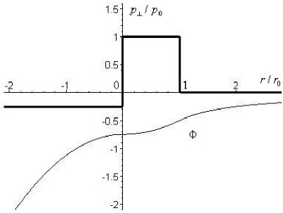
Figure 3: An asymmetric profile of the transversal pressure (in bold) inverting collapse into cosmological expansion that is asymptotically de-Sitter one. The thin line shows evolution of gravitational potential. This plot corresponds to the model in which the matter entirely fills $T$-region of the black hole ($r_{0}=2GM$). Besides, as an example, we set $p_{1}/p_{0}=0,5$ (see Sec. 5).

Let us consider two toy examples of the $p_{\perp}$-function behavior (Figs. 3, 4):

• an asymmetric step,  $p_{\perp}^{\left(A\right)}=p_{0}\cdot\theta\left(rr_{0}-r^{2}\right)-p_{1}\cdot\theta\left(-r\right),$

• a symmetric step,  $p_{\perp}^{\left(B\right)}=p_{0}\cdot\theta\left(r_{0}^{2}-r^{2}\right),$

where $r_{0}\leq 2GM$ and $p_{1}$  are positive real constants, $M\equiv 8\pi r_{0}^{3}p_{0}/3\,$ – the black-hole mass. Integrating eq. (6) with initial condition $\varepsilon(r\geq r_{0})=0$ yields the following functions $\varepsilon(r)$:

$$\varepsilon^{\left(A\right)}=-p_{\perp}^{\left(A\right)}+p_{0}\frac{r_{0}^{2}}{r^{2}}\cdot\theta\left(r_{0}-r\right),\qquad\varepsilon^{\left(B\right)}=p_{\perp}^{\left(B\right)}\cdot\left(\frac{r_{0}^{2}}{r^{2}}-1\right).$$ (7)

Thus, $(A)$ is a model of the astrogenic universe ($\varepsilon^{\left(A\right)}\rightarrow p_{1}$ as $r\rightarrow-\infty$) while $(B)$ is that of oscillating (eternal) black/white hole. The potential $\Phi(r)$ is of the $C^{1}$ class (see (4, 5), Figs. 3, 4).

Let us consider $(B)$ in two limits. As $r_{0}\rightarrow 0$ we obtain a black/white hole maximally extended onto the empty space with a delta-like source localized at $r=0$:

$$\varepsilon=2p_{\perp}=M\,\frac{\delta\left(r\right)}{2\pi r^{2}}\,,$$ (8)

where $\delta(r)=\theta^{\prime}(r)$ is one-dimensional delta-function.

In the limit $r_{0}=2GM$ we obtain a stationary black/white hole with an oscillating matter flow in the $T$-region:

$$r=-2GM\sin\left(H\tau\right)\,,\qquad\varepsilon=\frac{3H^{2}}{8\pi G}\,\cot^{2}\!\left(H\tau\right)\,,$$ (9)

$$ds^{2}=d\tau^{2}-\frac{1}{2}\left(\cos^{2}\!\left(H\tau\right)dt^{2}+\frac{\sin^{2}\!\left(H\tau\right)}{H^{2}}d\Omega\right),$$

where $H^{-1}\equiv 2\sqrt{2}GM$ and $\tau$ are the oscillation frequency and proper time of the flow, respectively.

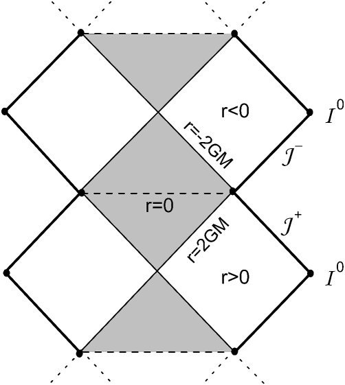
Figure 5: Penrose diagram of the pulsating flow with the symmetric function $p_{\perp}(r)$ (see Fig. 4). The matter occupies the shaded region.

Fig. 5 shows the Penrose diagram of this pulsating matter flow, spatially homogenous and anisotropic. Phase transitions in the matter on the stage of its expansion may, in principle, cause inflation and isotropize the flow to the Friedmannian symmetry in an arbitrary large volume.

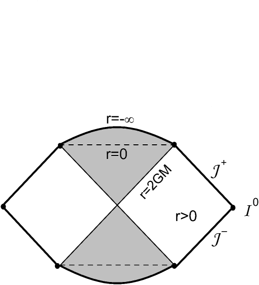
Figure 6: Penrose diagram of an astrogenic universe with the asymmetric function $p_{\perp}(r)$ (see Fig. 3).

The simplest realization of this scenario is exemplified by the case $(A)$. Indeed, if $\tau\geq 0$ eq. (7) yields the solution asymptotically approaching de-Sitter (see Fig. 6):

$$r=-\frac{\sinh(H_{1}\tau)}{\sqrt{2}H_{1}}\,,\qquad\varepsilon=\frac{3H^{2}_{1}}{8\pi G}\,\coth^{2}\!\left(H_{1}\tau\right),$$ (10)

$$ds^{2}=d\tau^{2}-\frac{1}{2}\left(\coth^{2}\!\left(H_{1}\tau\right)dt^{2}+\frac{\sinh^{2}\!\left(H_{1}\tau\right)}{H_{1}^{2}}d\Omega\right),$$

where the constant $H_{1}=(8\pi Gp_{1}/3)^{1/2}$ acquires any value independent of the external mass of the black hole. The presented toy model of astrogenic universe can be further elaborated by introducing massive scalar fields, radiation and the other ingredients of the contemporary CSM.

6 Conclusions

Extrapolation of the CSM to the past indicates that the initial Hubble matter flow expands from ultra-high curvature and density. In the models of black/white holes with integrable singularities the cosmological flows can emerge in the expanding white-hole $T$-regions lying in the absolute future with respect to the $T$-region of the maternal black hole. In the framework of this paradigm we introduce the notion of astrogenic cosmology, which is a cosmology originated from inversion of the collapse of some astrophysical compact system to expansion of the effective matter flow outside the body of the collapsed object. Figuratively speaking, black holes in these models are being lighters setting the new worlds on fire.

Multi-sheet universes with intricate topology predicted and discussed by A.D. Sakharov could have been realized through the collapse of compact systems on their final stages of evolution in a maternal universe. As mentioned above, a universe born as a result of this collapse needs to be isotropized (if we believe that this universe is similar to ours). The reason for that is a non-Friedmannian, though cosmological, symmetry of the interior of the white hole, namely, the cylindrical symmetry $\mathbb{R}\times\mathbb{S}^{2}$ of the Kantowski-Sachs model. Hence, residual cylindrical anisotropy in the present-day data would indicate the astrogenic mechanism of the beginning of our universe. Although some authors claim to have discovered a global anisotropy (see [14], for example), the current precision of cosmological observations is insufficient to state that, and future observations should clarify the situation.

7 Acknowledgements

The authors are grateful to the organizers of the Sakharov Session for the opportunity to present the talk and to P. B. Ivanov for critical reading of the manuscript. This work was partly supported by the Russian Foundation for Basic Research (project codes 11-02-12168-OFI-M-2011, 11-02-00244) and by the grant of Ministry of Science and Education of the Russian Federation (no. 16.740.11.0460). VNS also thanks the Dynasty Foundation for financial support.

Appendix

Recall [4] that  $q_{S}=\delta a/a+Hv$  where  $v$ are perturbations of the comoving scale factor and velocity potential of the matter, respectively. $q_{T}=(q_{\lambda})$ are amplitudes of gravitational waves with polarizations $\lambda=\oplus,\otimes$. The conformal fields $\tilde{q}={\tilde{\alpha}}q/\sqrt{8\pi G}$ obey the equations of classical harmonic oscillators with variable frequencies:

$${\tilde{q}}^{\,\prime\prime}+\left(\omega^{2}-U\right){\tilde{q}}=0\,,$$ (11)

where the prime stands for derivative with respect to the conformal time $\eta=\int dt/a$,

$$U\equiv\frac{{\tilde{\alpha}}^{\prime\prime}}{\tilde{\alpha}\;}\,,\qquad U_{T}=\left(2-\gamma\right)\!a^{2}H^{2}\,,\qquad{\tilde{\alpha}}_{S}=\frac{a\sqrt{2\gamma}}{\beta}\,,\qquad{\tilde{\alpha}}_{T}=a\,,$$

$\omega=\beta k,\;\beta_{S}$ – is the sound speed in the speed-of-light units, $\beta_{T}=1$. In the case when more than one medium is present the right-hand side of the $S$-oscillator equations acquires an additional term describing the action of isocurvature perturbations.

The dependence of the effective frequency ($\omega^{2}-U$) on time causes parametric amplification of the elementary oscillators in the course of the universe evolution. Assuming the vacuum initial state in the wave zone ($\omega^{2}>|U|$) and taking into account that the latter then turns into the parametric one ($|U|>\omega^{2}$) we obtain the solution of (11) in the form:

$$\frac{\exp{\left(-i\int\omega d\eta\right)}}{{\tilde{\alpha}}\sqrt{2\omega}}\,\rightarrow\,\frac{{\mathfrak{c}}-i}{C\sqrt{2k}}\,\rightarrow\,\frac{M_{P}\sqrt{\pi}}{2k^{3/2}}\,q_{k}\,,$$ (12)

where $C$ is a junction constant in the region $|U|\simeq\omega$ ,  the function ${\mathfrak{c}}=-kC^{2}\!\int{\tilde{\alpha}}^{-2}d\eta\rightarrow const$ converges at the upper limit if $\gamma<3$. The “frozen” fields $q_{k}=const(\eta)$ correspond to the growing mode of the general solution. Their phases are random while their absolute values give the spectral amplitudes $S=|q_{kS}|^{2}$ $T=|q_{k\oplus}|^{2}+|q_{k\otimes}|^{2}$. When $\beta=1$ and $\gamma\simeq const$ eqs. (11) are identical for either mode and $T/S=2{\tilde{\alpha}}_{S}^{2}/{\tilde{\alpha}}_{T}^{2}=4\gamma$. If $\gamma<1$ we obtain the $T$-spectrum (2) within a multiplicative factor of the order of unity.

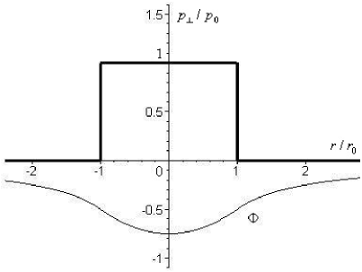
Figure 4: A symmetric profile of the transversal pressure (in bold) turning the black hole into a white hole of the same mass. The thin line shows the evolution of gravitational potential. The matter entirely fills $T$-regions of both black and white holes ($r_{0}=2GM$).

References

- [1] Sakharov A D, Sov. Phys. JETP 56, 705 (1982)
- [2] Sakharov A D, Sov. Phys. JETP 60, 214 (1984)
- [3] Carr B, Universe or Multiverse? Cambridge University Press: Cambridge (2007)
- [4] Lukash V N, Mikheeva E V, Physical cosmology, Fizmatlit: Moscow (2010). In Russian
- [5] Lukash V N, Strokov V N, arxiv.org: 1109.2796
- [6] Lifshiz E M, Zh. Eksp. Teor. Fiz. 16, 587 (1946)
- [7] Lukash V N, JETP Letters 31, 596 (1980); Sov. Phys. JETP 52, 807 (1980)
- [8] Guth A H, Phys. Rev. D 23 347 (1981)
- [9] Linde A D, Phys. Lett. B 108 389 (1982)
- [10] Dolgov A D, Sazhin M V, Zel’dovich Ya B, Basics of Modern Cosmology, Editions Frontieres: Gif-sur-Yvette, France (1990)
- [11] The Future of Theoretical Physics and Cosmology, edited by G W Gibbons, E P S Shellard, and S J Rankin, Cambridge University Press: Cambridge (2003)
- [12] Starobinsky A A, Phys. Lett B 91 99 (1980)
- [13] Novikov I D, Sov. Astron. 5 733 (1962)
- [14] P Erdogdu et al. MNRAS 368 1515 (2006); F K Hansen et al. Astrophys. J. 704 1448 (2009)