CTL Model Update for System Modifications

Abstract

Model checking is a promising technology, which has been applied for verification of many hardware and software systems. In this paper, we introduce the concept of model update towards the development of an automatic system modification tool that extends model checking functions. We define primitive update operations on the models of Computation Tree Logic (CTL) and formalize the principle of minimal change for CTL model update. These primitive update operations, together with the underlying minimal change principle, serve as the foundation for CTL model update. Essential semantic and computational characterizations are provided for our CTL model update approach. We then describe a formal algorithm that implements this approach. We also illustrate two case studies of CTL model updates for the well-known microwave oven example and the Andrew File System 1, from which we further propose a method to optimize the update results in complex system modifications.

1 Introduction

Model checking is one of the most effective technologies for automatic system verifications. In the model checking approach, the system behaviours are modeled by a Kripke structure, and specification properties that we require the system to meet are expressed as formulas in a propositional temporal logic, e.g., CTL. Then the model checker, e.g., SMV, takes the Kripke model and a formula as input, and verifies whether the formula is satisfied by the Kripke model. If the formula is not satisfied in the Kripke model, the system will report errors, and possibly provides useful information (e.g., counterexamples).

Over the past decade, the model checking technology has been considerably developed, and many effective model checking tools have been demonstrated through provision of thorough automatic error diagnosis in complex designs e.g., (?, ?, ?, ?, ?). Some current state-of-the-art model checkers, such as SMV (?), NuSMV (?) and Cadence SMV (?), employ SMV specification language for both Computational Tree Logic (CTL) and Linear Temporal Logic (LTL) variants (?, ?). Other model checkers, such as SPIN (?), use Promela specification language for on-the-fly LTL model checking. Additionally, the MCK (?) model checker was developed by integrating a knowledge operator into CTL model checking to verify knowledge-related properties of security protocols.

Although model checking approaches have been used for verification of problems in large complex systems, one major limitation of these approaches is that they can only verify the correctness of a system specification. In other words, if errors are identified in a system specification by model checking, the task of correcting the system is completely left to the system designers. That is, model checking is generally used only to verify the correctness of a system, not to modify it. Although the idea of repair has been indeed proposed for model-based diagnosis, repairing a system is only possible for specific cases (?, ?).

1.1 Motivation

Since model checking can handle complex system verification problems and as it may be implemented via fast algorithms, it is quite natural to consider whether we can develop associated algorithms so that they can handle system modification as well. The idea of integrating model checking and automatic modification has been investigated in recent years. Buccafurri, Eiter, Gottlob, and Leone (?) have proposed an approach whereby AI techniques are combined with model checking such that the enhanced algorithm can not only identify errors for a concurrent system, but also provide possible modifications for the system.

In the above approach, a system is described as a Kripke structure $M$, and a modification $\Gamma$ for $M$ is a set of state transitions that may be added to or removed from $M$. If a CTL formula $\varphi$ is not satisfied in $M$ i.e., the system contains errors with respect to property $\varphi$, then $M$ will be repaired by adding new state transitions or removing existing ones specified in $\Gamma$. As a result, the new Kripke structure $M^{\prime}$ will then satisfy formula $\varphi$. The approach of Buccafurri et al. (?) integrates model checking and abductive theory revision to perform system repairs. They also demonstrate how their approach can be applied to repair concurrent programs.

It has been observed that this type of system repair is quite restricted, as only relation elements (i.e., state transitions) in a Kripke model can be changed. This implies that errors can only be fixed by changing system behaviors. In fact, as we will show in this paper, allowing change to both states and relation elements in a Kripke structure significantly enhances the system repair process in most situations. Also, since providing all admissible modifications (i.e., the set $\Gamma$) is a pre-condition of any repair, the approach of Buccafurri et al. lacks flexibility. Indeed, as stated by the authors themselves, their approach may not be general enough for other system modifications.

On the other hand, knowledge-base update has been the subject of extensive study in the AI community since the late 1980s. Winslett’s Possible Model Approach (PMA) is viewed as pioneering work towards a model-based minimal change approach for knowledge-base update (?). Many researchers have since proposed different approaches to knowledge system update (e.g., see references from Eiter & Gottlob, 1992; Herzig & Rifi, 1999). Of these works, Harris and Ryan (?, ?) considered using an update approach for system modification, where they designed update operations to tackle feature integration, performing theory change and belief revision. However, their study focused mainly on the theoretical properties of system update, and practical implementation of their approach in system modification remains unclear.

Baral and Zhang (?) recently developed a formal approach to knowledge update based on single-agent S5 Kripke structures observing that system modification is closely related to knowledge update. From the knowledge dynamics perspective, we can view the finite transition system, which represents a real time complex system, to be a model of a knowledge set (i.e., a Kripke model). Thus the problem of system modification is reduced to the problem of updating this model so that a new updated model satisfies the knowledge formula.

This observation motivated the initial development of a general approach to updating Kripke models, which can be integrated into model checking technology, towards a more general automatic system modification. Ding and Zhang’s work (?) may be viewed as the first attempt to apply this idea to LTL model update. The LTL model update modifies the existing LTL model of an abstracted system to automatically correct the errors occurring within this model.

Based on the investigation described above, we intend to integrate knowledge update and CTL model checking to develop a practical model updater, which represents a general method for automatic system repairs.

1.2 Contributions of This Paper

The overall aim of our work is to design a model updater that improves model checking function by adding error repair (see schematic in Figure 1). The outcome from the updater is a corrected Kripke model. The model updater’s function is to automatically correct errors reported (possibly as counterexamples) by a model checking compiler. Eventually, the model updater is intended to be a universal compiler that can be used in certain common situations for model error detection and correction.

Figure 1: CTL model update.

The main contributions of this paper are described as follows:

1. We propose a formal framework for CTL model update. Firstly, we define primitive CTL model update operations and, based on these operations, specify a minimal change principle for the CTL model update. We then study the relationship between the proposed CTL model update and traditional propositional belief update. Interestingly, we prove that our CTL model update obeys all Katsuno and Mendelzon update postulates (U1) - (U8). We further provide important characterizations for special CTL model update formulas such as $\mbox{EX}\phi$, $\mbox{AG}\phi$ and $\mbox{EG}\phi$. These characterizations play an important role in optimization of the update procedure. Finally, we study the computational properties of CTL model update and show that, in general, the model checking problem for CTL model update is co-NP-complete. We also classify a useful subclass of CTL model update problems that can be performed in polynomial time.

2. We develop a formal algorithm for CTL model update. In principle, our algorithm can perform an update on a given CTL Kripke model with an arbitrary satisfiable CTL formula and generate a model that satisfies the input formula and has a minimal change with respect to the original model. The model then can be viewed as a possible correction on the original system specification. Based on this algorithm, we implement a system prototype of CTL model updater in C code in Linux.

3. We demonstrate important applications of our CTL model update approach by two case studies of the well-known microwave oven example (?) and the Andrew File System 1 (?). Through these case studies, we further propose a new update principle of minimal change with maximal reachable states, which can significantly improve the update results in complex system modification scenarios.

In summary, our work presented in this paper is an initial step towards the formal study of the automatic system modification. This approach may be integrated into existing model checkers so that we may develop a unified methodology and system for model checking and model correction. In this sense, our work will enhance the current model checking technology. Some results presented in this paper were published in ECAI 2006 (?).

The rest of the paper is organized as follows. An overview of CTL syntax and semantics is provided in Section 2.1. Primitive update operations on CTL models are defined in Section 3, and a minimal change principle for CTL model update is then developed. Section 4 consists of a study of the relationship between CTL model update and Katsuno and Mendelzon’s update postulates (U1) - (U8), and various characterizations for some special CTL model updates. In Section 5, a general computational complexity result of CTL model update is proved, and a useful tractable subclass of CTL model update problems is identified. A formal algorithm for the proposed CTL model update approach is described in Section 6. In Section 7, two update case studies are illustrated to demonstrate applications of our CTL model update approach. Section 8 proposes an improved CTL model update approach which can significantly optimize the update results in complex system modification scenarios. Finally, the paper concludes with some future work discussions in Section 9.

2 Preliminaries

In this section, we briefly review the syntax and semantics of Computation Tree Logic and basic concepts of belief update, which are the foundation for our CTL model update.

2.1 CTL Syntax and Semantics

To begin with, we briefly review CTL syntax and semantics (refer to ? and ? for details).

Definition 1

Let $AP$ be a set of atomic propositions. A Kripke model $M$ over AP is a triple $M=(S,R,L)$ where:

1. $S$ is a finite set of states;

2. $R\subseteq S\times S$ is a binary relation representing state transitions;

3. $L:S\rightarrow 2^{AP}$ is a labeling function that assigns each state with a set of atomic propositions.

An example of a finite Kripke model is represented by the graph in Figure 2, where each node represents a state in $S$, which is attached to a set of propositional atoms being assigned by the labeling function, and an edge represents a state transition - a relation element in $R$ describing a system transition from one state to another.

Figure 2: Transition state graph.

Computation Tree Logic (CTL) is a temporal logic allowing us to refer to the future. It is also a branching-time logic, meaning that its model of time is a tree-like structure in which the future is not determined but consists of different paths, any one of which might be the ‘actual’ path that is eventually realized (?).

Definition 2

CTL has the following syntax given in Backus-Naur form:

$\phi::=\top\mid\perp\mid p\mid(\neg\phi)\mid(\phi_{1}\wedge\phi_{2})\mid(\phi_{1}\vee\phi_{2})\mid\phi\rightarrow\psi\mid\mbox{\em AX}\phi\mid\mbox{\em EX}\phi$

$\mid\mbox{\em AG}\phi\mid\mbox{\em EG}\phi\mid\mbox{\em AF}\phi\mid\mbox{\em EF}\phi\mid\mbox{\em A}[\phi_{1}\mbox{\em U}\phi_{2}]\mid\mbox{\em E}[\phi_{1}\mbox{\em U}\phi_{2}]$

where $p$ is any propositional atom.

A CTL formula is evaluated on a Kripke model. A path in a Kripke model from a state is a(n) (infinite) sequence of states. Note that for a given path, the same state may occur an infinite number of times in the path (i.e., the path contains a loop). To simplify our following discussions, we may identify states in a path with different position subscripts, although states occurring in different positions in the path may be the same. In this way, we can say that one state precedes another in a path without much confusion. Now we can present useful notions in a formal way. Let $M=(S,R,L)$ be a Kripke model and $s\in S$. A path in $M$ starting from $s$ is denoted as $\pi=[s_{0},s_{1},\cdots,s_{i-1},s_{i},s_{i+1},\cdots]$, where $s_{0}=s$ and $(s_{i},s_{i+1})\in R$ holds for all $i\geq 0$. We write $s_{i}\in\pi$ if $s_{i}$ is a state occurring in the path $\pi$. If a path $\pi=[s_{0},s_{1},\cdots,s_{i},\cdots,s_{j},\cdots]$ and $i<j$, we also denote $s_{i}<s_{j}$. Furthermore for a given path $\pi$, we use notion $s\leq s_{i}$ to denote a state $s$ that is the state $s_{i}$ or $s<s_{i}$. For simplicity, we may use $succ(s)$ to denote state $s^{\prime}$ if there is a relation element $(s,s^{\prime})$ in $R$.

Definition 3

Let $M=(S,R,L)$ be a Kripke model for CTL. Given any $s$ in $S$, we define whether a CTL formula $\phi$ holds in $M$ at state $s$. We denote this by $(M,s)\models\phi$. The satisfaction relation $\models$ is defined by structural induction on all CTL formulas:

1. $(M,s)\models\top$ and $(M,s)\not\models\perp$ for all $s\in S$.

2. $(M,s)\models p$ iff $p\in L(s)$.

3. $(M,s)\models\neg\phi$ iff $(M,s)\not\models\phi$.

4. $(M,s)\models\phi_{1}\wedge\phi_{2}$ iff $(M,s)\models\phi_{1}$ and $(M,s)\models\phi_{2}$.

5. $(M,s)\models\phi_{1}\vee\phi_{2}$ iff $(M,s)\models\phi_{1}$ or $(M,s)\models\phi_{2}$.

6. $(M,s)\models\phi_{1}\rightarrow\phi_{2}$ iff $(M,s)\models\neg\phi_{1}$, or $(M,s)\models\phi_{2}$.

7. $(M,s)\models\mbox{\em AX}\phi$ iff for all $s_{1}$ such that $(s,s_{1})\in R$, $(M,s_{1})\models\phi$.

8. $(M,s)\models\mbox{\em EX}\phi$ iff for some $s_{1}$ such that $(s,s_{1})\in R$, $(M,s_{1})\models\phi$.

9. $(M,s)\models\mbox{\em AG}\phi$ iff for all paths $\pi=[s_{0},s_{1},s_{2},\cdots]$ where $s_{0}=s$ and $\forall s_{i},~{}s_{i}\in\pi$, $(M,s_{i})\models\phi$.

10. $(M,s)\models\mbox{\em EG}\phi$ iff there is a path $\pi=[s_{0},s_{1},s_{2},\cdots]$ where $s_{0}=s$ and $\forall s_{i},~{}s_{i}\in\pi$, $(M,s_{i})\models\phi$.

11. $(M,s)\models\mbox{\em AF}\phi$ iff for all paths $\pi=[s_{0},s_{1},s_{2},\cdots]$ where $s_{0}=s$ and $\exists s_{i},~{}s_{i}\in\pi$, $(M,s_{i})\models\phi$.

12. $(M,s)\models\mbox{\em EF}\phi$ iff there is a path $\pi=[s_{0},s_{1},s_{2},\cdots]$ where $s_{0}=s$ and $\exists s_{i},~{}s_{i}\in\pi$, $(M,s_{i})\models\phi$.

13. $(M,s)\models\mbox{\em A}[\phi_{1}\mbox{\em U}\phi_{2}]$ iff for all paths $\pi=[s_{0},s_{1},s_{2},\cdots]$ where $s_{0}=s$, $\exists s_{i}\in\pi$, $(M,s_{i})\models\phi_{2}$ and for each $j<i$, $(M,s_{j})\models\phi_{1}$.

14. $(M,s)\models\mbox{\em E}[\phi_{1}\mbox{\em U}\phi_{2}]$ iff there is a path $\pi=[s_{0},s_{1},s_{2},\cdots]$ where $s_{0}=s$, $\exists s_{i}\in\pi$, $(M,s_{i})\models\phi_{2}$ and for each $j<i$, $(M,s_{j})\models\phi_{1}$.

From the above definition, we can see that the intuitive meaning of A, E, X, and G are quite clear: A means for all paths, E means that there exists a path, X refers to the next state and G means for all states globally. Then the semantics of a CTL formula is easy to capture as follows.

In the first six clauses, the truth value of the formula in the state depends on the truth value of $\phi_{1}$ or $\phi_{2}$ in the same state. For example, the truth value of $\neg\phi$ in a state only depends on the truth value of $\phi$ in the same state. This contrasts with clauses $7$ and $8$ for AX and EX. For instance, the truth value of AX$\phi$ in a state $s$ is determined not by $\phi$’s truth value in $s$, but by $\phi$’s truth values in states $s^{\prime}$ where $(s,s^{\prime})\in R$; if $(s,s)\in R$, then this value also depends on the truth value of $\phi$ in $s$.

The next four clauses ($9$ - $12$) also exhibit this phenomenon. For example, the truth value of AG$\phi$ involves looking at the truth value of $\phi$ not only in the immediately related states, but in indirectly related states as well. In the case of AG$\phi$, we must examine the truth value of $\phi$ in every state related by any number of forward links (paths) to the current state $s$. In clauses $13$ and $14$, symbol U may be explained as “until”: a path $\pi=[s_{0},s_{1},s_{2},\cdots]$ satisfies $\phi_{1}\mbox{U}\phi_{2}$ if there is a state $s_{i}\in\pi$ such that for all $s<s_{i}$, $(M,s)\models\phi_{1}$ until $(M,s_{i})\models\phi_{2}$.

Clauses $9$ - $14$ above refer to computation paths in models. It is, therefore, useful to visualize all possible computation paths from a given state $s$ by unwinding the transition system to obtain an infinite computation tree. This greatly facilitates deciding whether a state satisfies a CTL formula. The unwound tree of the graph in Figure 2 is depicted in Figure 3 (note that we assume $s_{0}$ is the initial state in this Kripke model).

Figure 3: Unwinding the transition state graph as an infinite tree.

In Figure 3, if $\phi=r$, then AX$r$ is true; if $\phi=q$, then EX$q$ is true. In the same figure, if $\phi=r$, then AF$r$ is true because some states on all paths will satisfy $r$ some time in the future. If $\phi=q$, EF$q$ is true because some states on some paths will satisfy $q$ some time in the future. The clauses for AG and EG can be explained in Figure 4. In this tree, all states satisfy $r$. Thus, AG$r$ is true in this Kripke model. There is one path where all states satisfy $\phi=q$. Thus, EG$q$ is true in this Kripke model.

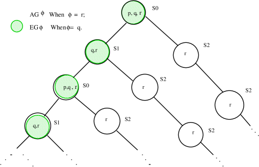
Figure 4: AG$\phi$ and EG$\phi$ in an unwound tree.

The following De Morgan rules and equivalences (?) will be useful for our CTL model update algorithm implementation:

$$\neg\mbox{AF}\phi\equiv\mbox{EG}\neg\phi;$$

$$\neg\mbox{EF}\phi\equiv\mbox{AG}\neg\phi;$$

$$\neg\mbox{AX}\phi\equiv\mbox{EX}\neg\phi;$$

$$\mbox{AF}\phi\equiv\mbox{A}[\top\mbox{U}\phi];$$

$$\mbox{EF}\phi\equiv\mbox{E}[\top\mbox{U}\phi];$$

$$\mbox{A}[\phi_{1}\mbox{U}\phi_{2}]\equiv\neg(\mbox{E}[\neg\phi_{2}\mbox{U}(\neg\phi_{1}\wedge\phi_{2})]\vee\mbox{EG}\neg\phi_{2}).$$

In the rest of this paper, without explicit declaration, we will assume that all CTL formulas occurring in our context will be satisfiable. For instance, if we consider updating a Kripke model to satisfy a CTL formula $\phi$, we already assume that $\phi$ is satisfiable.

From Definition 3, we can see that for a given CTL Kripke model $M=(S,R,L)$, if $(M,s)\models\phi$ and $\phi$ is a propositional formula, then $\phi$’s truth value solely depends on the labeling function $L$’s assignment on state $s$. In this case we may simply write $L(s)\models\phi$ if there is no confusion from the context.

2.2 Belief Update

Belief change has been a primary research topic in the AI community for almost two decades e.g., (?, ?). Basically, it studies the problem of how an agent can change its beliefs when it wants to bring new beliefs into its belief set. There are two types of belief changes, namely belief revision and belief update. Intuitively, belief revision is used to modify a belief set in order to accept new information about the static world, while belief update is to bring the belief set up to date when the world is described by its changes.

Katsuno and Mendelzon (?) have discovered that the original AGM revision postulates cannot precisely characterize the feature of belief update. They proposed the following alternative update postulates, and argued that any propositional belief update operators should satisfy these postulates. In the following (U1) - (U8) postulates, all occurrences of $T$, $\mu$, $\alpha$, etc. are propositional formulas.

(U1)  $T\diamond\mu\models\mu$.
(U2)  If $T\models\mu$ then $T\diamond\mu\equiv T$.
(U3)  If both $T$ and $\mu$ are satisfiable then $T\diamond\mu$ is also satisfiable.
(U4)  If $T_{1}\equiv T_{2}$ and $\mu_{1}\equiv\mu_{2}$ then $T\diamond\mu_{1}\equiv T_{2}\diamond\mu_{2}$.
(U5)  $(T\diamond\mu)\wedge\alpha\models T\diamond(\mu\wedge\alpha)$.
(U6)  If $T\diamond\mu_{1}\models\mu_{2}$ and $T\diamond\mu_{2}\models\mu_{1}$ then $T\diamond\mu_{1}\equiv T\diamond\mu_{2}$.
(U7)  If $T$ is complete (i.e., has a unique model) then
        $(T\diamond\mu_{1})\wedge(T\diamond\mu_{2})\models T\diamond(\mu_{1}\vee\mu_{2})$.
(U8)  $(T_{1}\vee T_{2})\diamond\mu\equiv$ $(T_{1}\diamond\mu)\vee(T_{2}\diamond\mu)$.

As shown by Katsuno and Mendelzon (?), postulates (U1) - (U8) precisely capture the minimal change criterion for update that is defined based on certain partial ordering on models. As a typical model based belief update approach, here we briefly introduce Winslett’s Possible Models Approach (PMA) (?). We consider a propositional language ${\mathcal{L}}$. Let $I_{1}$ and $I_{2}$ be two Herband interpretations of ${\mathcal{L}}$. The symmetric difference between $I_{1}$ and $I_{2}$ is defined as $diff(I_{1},I_{2})=(I_{1}-I_{2})\cup(I_{2}-I_{1})$. Then for a given interpretation $I$, we define a partial ordering $\leq_{I}$ as follows: $I_{1}\leq_{I}I_{2}$ if and only if $diff(I,I_{1})\subseteq diff(I,I_{2})$. Let ${\mathcal{I}}$ be a collection of interpretations, we denote $Min({\mathcal{I}},\leq_{M})$ to be the set of all minimal models from ${\mathcal{I}}$ with respect to ordering $\leq_{M}$, where model $M$ is fixed. Now let $\phi$ and $\mu$ be two propositional formulas, the update of $\phi$ with $\mu$ using the PMA, denoted as $\phi\diamond_{pma}\mu$, is defined as follows:

$Mod(\phi\diamond_{pma}\mu)=\bigcup_{M\in Mod(\phi)}Min(Mod(\mu),\leq_{M})$,

where $Mod(\psi)$ denotes the set of all models of formula $\psi$. It can be proved that the PMA update operator $\diamond_{pma}$ satisfies all postulates (U1) - (U8).

Our work of CTL model update has a close connection to the idea of belief update. As will be shown in this paper, in our approach, we view a CTL Kripke model as a description of the world that we are interested in, i.e., the description of a system of dynamic behaviours, and the update on this Kripke model occurs when the setting of the system of dynamic behaviours has to change to accommodate some desired properties. Although there is a significant difference between classical propositional belief update and our CTL model update, we will show that Katsuno Mendelzon’s update postulates (U1) - (U8) are also suitable to characterize the minimal change principle for our CTL model update.

3 Minimal Change for CTL Model Update

We would like to extend the idea of minimal change in belief update to our CTL model update. In principle, when we need to update a CTL Kripke model to satisfy a CTL formula, we expect the updated model to retain as much information as possible represented in the original model. In other words, we prefer to change the model in a minimal way to achieve our goal. In this section, we will propose formal metrics of minimal change for CTL model update.

3.1 Primitive Update Operations

Given a CTL Kripke model and a (satisfiable) CTL formula, we consider how this model can be updated in order to satisfy the given formula. From the discussion in the previous section, we try to incorporate a minimal change principle into our update approach. As the first step towards this aim, we should have a way to measure the difference between two CTL Kripke models in relation to a given model. We first illustrate our initial consideration of this aspect through an example.

Example 1

Consider a simple CTL model $M=(\{s_{0},s_{1},s_{2}\},\{(s_{0},s_{0})$, $(s_{0},s_{1})$, $(s_{0},s_{2})$, $(s_{1},s_{1})$, $(s_{2},s_{2})$, $(s_{2},s_{1})\},L)$, where $L(s_{0})=\{p,q\},L(s_{1})=\{q,r\}$ and $L(s_{2})=\{r\}$. $M$ is described as in Figure 5.

Figure 5: Model $M$.

Now consider formula AG$p$. Clearly, $(M,s_{0})\not\models$ AG$p$. One way to update $M$ to satisfy AG$p$ is to update states $s_{1}$ and $s_{2}$ so that both updated states satisfy $p$. Therefore, we obtain a new CTL model $M^{\prime}=(\{s_{0},s_{1},s_{2}\},\{(s_{0},s_{0}),(s_{0},s_{1}),(s_{0},s_{2})$, $(s_{1},s_{1})$, $(s_{2},s_{2})$, $(s_{2},s_{1})\}$, $L^{\prime})$, where $L^{\prime}(s_{0})=L(s_{0})=\{p,q\},L^{\prime}(s_{1})=\{p,q,r\}$ and $L^{\prime}(s_{2})=\{p,r\}$. In this update, we can see that the labeling function has been changed to associate different truth assignments with states $s_{1}$ and $s_{2}$. Another way to update $M$ to satisfy formula AG$p$ is to simply remove relation elements $(s_{0},s_{1})$ and $(s_{0},s_{2})$ from $M$, this gives $(M^{\prime\prime},s_{0})\models$ AG$p$, where $M^{\prime\prime}=(\{s_{0},s_{1},s_{2}\},\{(s_{0},s_{0}),(s_{1},s_{1}),(s_{2},s_{2}),(s_{2},s_{1})\},L)$. This more closely resembles the approach of Buccafurri et al.  (?), where no state changes occur. It is interesting to note that the first of the updated models retains the same “structure” as the original, while it is significantly changed in the second. These two possible results are described in Figure 6. $\Box$

Figure 6: Two possible results of updating $M$ with AG$p$.

The above example shows that in order to update a CTL model to satisfy a formula, we may apply different kinds of operations to change the model. From all possible operations applicable to a CTL model, we consider five basic ones where all changes on a CTL model can be achieved.

PU1: Adding one relation element
Given $M=(S,R,L)$, its updated model $M^{\prime}=(S^{\prime},R^{\prime},L^{\prime})$ is obtained from $M$ by adding only one new relation element. That is, $S^{\prime}=S$, $L^{\prime}=L$, and $R^{\prime}=R\cup\{(s_{i},s_{j})\}$, where $(s_{i},s_{j})\not\in R$ for two states $s_{i},s_{j}\in S$.

PU2: Removing one relation element
Given $M=(S,R,L)$, its updated model $M^{\prime}=(S^{\prime},R^{\prime},L^{\prime})$ is obtained from $M$ by removing only one existing relation element. That is, $S^{\prime}=S$, $L^{\prime}=L$, and $R^{\prime}=R-\{(s_{i},s_{j})\}$, where $(s_{i},s_{j})\in R$ for two states $s_{i},s_{j}\in S$.

PU3: Changing labeling function on one state
Given $M=(S,R,L)$, its updated model $M^{\prime}=(S^{\prime},R^{\prime},L^{\prime})$ is obtained from $M$ by changing labeling function on a particular state. That is, $S^{\prime}=S$, $R^{\prime}=R$, $\forall s\in(S-\{s^{*}\})$, $s^{*}\in S$, $L^{\prime}(s)=L(s)$, and $L^{\prime}(s^{*})$ is a set of true variable assigned in state $s^{*}$ where $L^{\prime}(s^{*})\neq L(s^{*})$.

PU4: Adding one state
Given $M=(S,R,L)$, its updated model $M^{\prime}=(S^{\prime},R^{\prime},L^{\prime})$ is obtained from $M$ by adding only one new state. That is, $S^{\prime}=S\cup\{s^{*}\}$, $s^{*}\not\in S$, $R^{\prime}=R$, and $\forall s\in S$, $L^{\prime}(s)=L(s)$ and $L^{\prime}(s^{*})$ is a set of true variables assigned in $s^{*}$.

PU5: Removing one isolated state
Given $M=(S,R,L)$, its updated model $M^{\prime}=(S^{\prime},R^{\prime},L^{\prime})$ is obtained from $M$ by removing only one isolated state: $S^{\prime}=S-\{s^{*}\}$, where $s^{*}\in S$ and $\forall s\in S$ such that $s\neq s^{*}$, neither $(s,s^{*})$ nor $(s^{*},s)$ is not in $R$, $R^{\prime}=R$, and $\forall s\in S^{\prime}$, $L^{\prime}(s)=L(s)$.

We call the above five operations primitive since they express all kinds of changes to a CTL model. Figure 7 illustrates examples of applying some of these operations on a model.

In the above five operations, PU1, PU2, PU4 and PU5 represent the most basic operations on a graph. Generally, using these four operations, we can perform any changes to a CTL model. For instance, if we want to substitute a state in a CTL model, we do the following: (1) remove all relation elements associated to this state, (2) remove this isolated states, (3) add a state that we want to replace the original one, and (4) add all relevant relation elements associated to this new state.

Although these four operations are sufficient enough to represent all changes on a CTL model, they sometimes complicate the measure on the changes of CTL models. Consider the case of a state substitution. Given a CTL model $M$, if one CTL model $M^{\prime}$ has exactly the same graphical structure as $M$ except that $M^{\prime}$ only has one particular state different from $M$, then we tend to think that $M^{\prime}$ is obtained from $M$ with a single change of state replacement, instead of from a sequence of operations PU1, PU2, PU4 and PU5.

This motivates us to have operation PU3. PU3 has an effect of state substitution, but it is fundamentally different from the combination of PU1, PU2, PU4 and PU5, because PU3 does not change the state name and relation elements in the original model, it only assigns a different set of propositional atoms to that state in the original model. In this sense, the combination of PU1, PU2, PU4 and PU5 cannot replace operation PU3. Using PU3 to represent state substitution significantly simplifies our measure on the model difference as will be illustrated in Definition 4. In the rest of the paper, we assume that all state substitutions in a CTL model will be achieved through PU3 so that we have a unique way to measure the differences on CTL model changes in relation to states substitutions.

We should also note that having operation PU3 as a way to substitute a state in a CTL model, PU5 becomes unnecessary, because we actually do not need to remove an isolated state from a model. All we need is to remove relevant relation element(s) in the model, so that this state becomes unreachable from the initial state. Nevertheless, to remain our discussions to be coherent with all primitive operations described above, in the following definition on the CTL minimal change, we still consider the measure on changes caused by applying PU5 in a CTL model update.

Figure 7: Illustration of primitive updates.

3.2 Defining Minimal Change

Following traditional belief update principle, in order to make a CTL model to satisfy some property, we would expect that the given CTL model is changed as little as possible. By using primitive update operations, a CTL Kripke model may be updated in different ways: adding or removing state transitions, adding new states, and changing the labeling function for some state(s) in the model. Therefore, we first need to have a method to measure the changes of CTL models, from which we can develop a minimal change criterion for CTL model update.

Given two CTL models $M=(S,R,L)$ and $M^{\prime}=(S^{\prime},R^{\prime},L^{\prime})$, for each operation $PUi$ ($i=1,\cdots,5$), ${\mathit{D}iff}_{PUi}(M,M^{\prime})$ denotes the differences between the two models where $M^{\prime}$ is an updated model from $M$, which makes clear that several operations of type $PUi$ have occurred. Since PU1 and PU2 only change relation elements, we define ${\mathit{D}iff}_{PU1}(M,M^{\prime})=R^{\prime}-R$ (adding relation elements only) and ${\mathit{D}iff}_{PU2}(M,M^{\prime})=R-R^{\prime}$ (removing relation elements only). For operation PU3, since only labeling function is changed, the difference measure between $M$ and $M^{\prime}$ for PU3 is defined as ${\mathit{D}iff}_{PU3}(M,M^{\prime})=\{s\mid s\in S\cap S^{\prime}$ and $L(s)\neq L^{\prime}(s)\}$. For operations PU4 and PU5, on the other hand, we define ${\mathit{D}iff}_{PU4}(M,M^{\prime})=S^{\prime}-S$ (adding states) and ${\mathit{D}iff}_{PU5}(M,M^{\prime})=S-S^{\prime}$ (removing states). Let ${\mathcal{M}}=(M,s)$ and ${\mathcal{M}^{\prime}}=(M^{\prime},s^{\prime})$, for convenience, we also denote ${\mathit{D}iff}({\mathcal{M}},{\mathcal{M}^{\prime}})$ $=$ $({\mathit{D}iff}_{PU1}(M,M^{\prime}),{\mathit{D}iff}_{PU2}(M,M^{\prime}),{\mathit{D}iff}_{PU3}(M,M^{\prime}),{\mathit{D}iff}_{PU4}(M,M^{\prime}),{\mathit{D}iff}_{PU5}(M,M^{\prime}))$.

It is worth mentioning that given two CTL Kripke models $M$ and $M^{\prime}$, there is no ambiguity to compute ${\mathit{D}iff}_{PUi}(M,M^{\prime})$ ($i=1,\cdots,5$), because each primitive operation will only cause one type of changes (states, relation elements, or labeling function) in the models no matter how many times it has been applied. Now we can precisely define the ordering $\leq_{M}$ on CTL models.

Definition 4

(Closeness ordering) Let $M$, $M_{1}$ and $M_{2}$ be three CTL Kripke models. We say that $M_{1}$ is at least as close to $M$ as $M_{2}$, denoted as $M_{1}\leq_{M}M_{2}$, if and only if for each set of PU1-PU5 operations that transform $M$ to $M_{2}$, there exists a set of PU1-PU5 operations that transform $M$ to $M_{1}$ such that the following conditions hold:

1. for each $i$ ($i=1,\cdots,5$), ${\mathit{D}iff}_{PUi}(M,M_{1})\subseteq{\mathit{D}iff}_{PUi}(M,M_{2})$, and

2. if ${\mathit{D}iff}_{PU3}(M,M_{1})={\mathit{D}iff}_{PU3}(M,M_{2})$, then for each $s\in{\mathit{D}iff}_{PU3}(M,M_{1})$,
   $diff(L(s),L_{1}(s))\subseteq diff(L(s),L_{2}(s))$.

We denote $M_{1}<_{M}M_{2}$ if $M_{1}\leq_{M}M_{2}$ and $M_{2}\not\leq_{M}M_{1}$.

Definition 4 presents a measure on the difference between two models with respect to a given model. Intuitively, we say that model $M_{1}$ is closer to $M$ relative to model $M_{2}$, if (1) $M_{1}$ is obtained from $M$ by applying all primitive update operations that cause fewer changes than those applied to obtain model $M_{2}$; and (2) if the set of states in $M_{1}$ affected by applying PU3 is the same as that in $M_{2}$, then we take a closer look at the difference on the set of propositional atoms associated with the relevant states. Having the ordering specified in Definition 4, we can define a CTL model update formally.

Definition 5

(Admissible update) Given a CTL Kripke model $M=(S,R,L)$, ${\mathcal{M}}=(M,s_{0})$ where $s_{0}\in S$, and a CTL formula $\phi$, a CTL Kripke model $Update({\mathcal{M}},\phi)$ is called an admissible model (or admissible updated model) if the following conditions hold: (1) $Update({\mathcal{M}},\phi)=(M^{\prime},s_{0}^{\prime})$, $(M^{\prime},s_{0}^{\prime})\models\phi$, where $M^{\prime}=(S^{\prime},R^{\prime},L^{\prime})$ and $s_{0}^{\prime}\in S^{\prime}$; and, (2) there does not exist another updated model $M^{\prime\prime}=(S^{\prime\prime},R^{\prime\prime},L^{\prime\prime})$ and $s_{0}^{\prime\prime}\in S^{\prime\prime}$ such that $(M^{\prime\prime},s_{0}^{\prime\prime})\models\phi$ and $M^{\prime\prime}<_{M}M^{\prime}$. We use ${\mathit{P}oss}(Update({\mathcal{M}},\phi))$ to denote the set of all possible admissible models of updating ${\mathcal{M}}$ to satisfy $\phi$.

Example 2

In Figure 8, model $M$ is updated in two different ways. Model $M_{1}$ is the result of updating $M$ by applying PU1. Model $M_{2}$ is another update of $M$ resulting by applying PU1, PU2 and PU5. Then we have ${\mathit{D}iff}_{PU1}(M,M_{1})=\{(s_{0},s_{2})\}$, and ${\mathit{D}iff}_{PU1}(M,M_{2})=\{(s_{1},s_{0}),(s_{0},s_{2})\}$, which results in ${\mathit{D}iff}_{PU1}(M,M_{1})\subset{\mathit{D}iff}_{PU1}(M,M_{2})$. Also, it is easy to see that ${\mathit{D}iff}_{PU2}(M,M_{1})=\emptyset$ and ${\mathit{D}iff}_{PU2}(M,M_{2})=\{(s_{3},s_{0}),(s_{2},s_{3})\}$, so ${\mathit{D}iff}_{PU2}(M,M_{1})$ $\subset$ ${\mathit{D}iff}_{PU2}(M,M_{2})$. Similarly, we can see that ${\mathit{D}iff}_{PU3}(M,M_{1})={\mathit{D}iff}_{PU3}(M,M_{2})=\emptyset$, and ${\mathit{D}iff}_{PU4}(M,M_{1})={\mathit{D}iff}_{PU4}(M,M_{2})=\emptyset$. Finally, we have ${\mathit{D}iff}_{PU5}(M,M_{1})=\emptyset$ and ${\mathit{D}iff}_{PU5}(M,M_{2})=\{s_{3}\}$. According to Definition 4, we have $M_{1}<_{M}M_{2}$. $\Box$

Figure 8: Illustration of minimal change rules.

We should note that in a CTL model update, if we can simply replace the initial state by another existing state in the model to satisfy the formula, then this model actually has not been changed, and it is the unique admissible model according to Definition 5. In this case, all other updates will be ruled out by Definition 5. For example, consider the CTL model $M$ described in Figure 9:

Figure 9: A special model update scenario.

If we want to update $(M,s_{0})$ with $\mbox{AX}p$, we can see that $(M,s_{1})$ becomes the only admissible updated model according to our definition: we simply replace the initial state $s_{0}$ by $s_{1}$. Nevertheless, we would expect that some other update may also be equally reasonable. For instance, we may change the labeling function of $M$ to make $L^{\prime}(s_{1})=\{p\}$. In both updates, we have changed something in $M$, but the change caused by the first update is not represented in our minimal change definition.

We can overcome this difficulty by creating a dummy state $\sharp$ into a CTL Kripke model $M$, and for each initial state $s$ in $M$, we add relation element $(\sharp,s)$ into $M$. In this way, a change of initial state from $s$ to $s^{\prime}$ will imply a removal of relation element $(\sharp,s)$ and an addition of a new relation element $(\sharp,s^{\prime})$. Such changes will be measured by our minimal change definition. With this treatment, both updated models described above are admissible. In the rest of the paper, without explicit declaration, we will assume that each CTL Kripke model contains a dummy state $\sharp$ and special state transitions from $\sharp$ to all initial states.

4 Semantic Properties

In this section, we first explore the relationship between our CTL model update and traditional belief update, and then provide useful semantic characterizations on some typical CTL model update cases.

4.1 Relationship to Propositional Belief Update

First we show the following result about ordering $\leq_{M}$ defined in Definition 4.

Proposition 1

$\leq_{M}$ is a partial ordering.

Proof: From Definition 4, it is easy to see that $\leq_{M}$ is reflexive and antisymmetric. Now we show that $\leq_{M}$ is also transitive. Suppose $M_{1}\leq_{M}M_{2}$ and $M_{2}\leq_{M}M_{3}$. According to Definition 4, we have $Diff_{PUi}(M,M_{1})\subseteq Diff_{PUi}(M,M_{2})$, and $Diff_{PUi}(M,M_{2})\subseteq Diff_{PUi}(M,M_{3})$ ($i=1,\cdots,5$). Consequently, we have $Diff_{PUi}(M,M_{1})\subseteq Diff_{PUi}(M,M_{3})$ ($i=1,\cdots,5$). So Condition 1 in Definition 4 holds. Now consider Condition 2 in the definition. The only case we need to consider is that $Diff_{PU3}(M,M_{1})=Diff_{PU3}(M,M_{2})$ and $Diff_{PU3}(M,M_{2})=Diff_{PU3}(M,M_{3})$ (note that all other cases will directly imply $Diff_{PU3}(M,M_{1})\subseteq Diff_{PU3}(M,M_{3})$ and $Diff_{PU3}(M,M_{1})\neq Diff_{PU3}(M,M_{3})$). In this case, it is obvious that for all $s\in Diff_{PU3}(M,M_{1})$ $=$ $Diff_{PU3}(M,M_{3})$, $diff(L(s),L_{1}(s))\subseteq diff(L(s),L_{3}(s))$. So we have $M_{1}\leq_{M}M_{3}$. $\Box$

It is also interesting to consider a special case of our CTL model update where the update formula is a classical propositional formula. The following proposition indicates that when only propositional formula is considered in CTL model update, the admissible model can be obtained through the traditional model based belief update approach (?).

Proposition 2

Let $M=(S,R,L)$ be a CTL model and $s_{0}\in S$. Suppose that $\phi$ is a satisfiable propositional formula and $(M,s_{0})\not\models\phi$, then an admissible model of updating $(M,s_{0})$ to satisfy $\phi$ is $(M^{\prime},s_{0})$, where $M^{\prime}=(S,R,L^{\prime})$, for each $s\in(S-\{s_{0}\})$, $L^{\prime}(s)=L(s)$, $L^{\prime}(s_{0})\models\phi$, and there does not exist another $M^{\prime\prime}=(S,R,L^{\prime\prime})$ such that $L^{\prime\prime}(s_{0})\models\phi$ and $diff(L(s_{0}),L^{\prime\prime}(s_{0}))\subset diff(L(s_{0}),L^{\prime}(s_{0}))$.

Proof: Since $\phi$ is a propositional formula, the update on $(M,s_{0})$ to satisfy $\phi$ will not affect any relation elements and all other states except $s_{0}$. Since $L(s_{0})\not\models\phi$, it is obvious that by applying PU3, we can change the labeling function $L$ to $L^{\prime}$ that assigns $s_{0}$ a new set of propositional atoms to satisfy $\phi$. Then from Definition 5, we can see that the model specified in the proposition is indeed a minimally changed CTL model with respect to ordering $\leq_{M}$. $\Box$

We can see that the problem addressed by our CTL model update is essentially different from the problem concerned in traditional propositional belief update. Nevertheless, the idea of model based minimal change for CTL model update is closely related to belief update. Therefore, it is worth investigating the relationship between our CTL model update and traditional propositional belief update postulates (U1) - (U8). In order to make such a comparison possible, we should lift the update operator occurring in postulates (U1) - (U8) beyond the propositional logic case.

For this purpose, we first introduce some notions. Given a CTL formula $\phi$ and Kripke model $M=(S,R,L)$, let $Init(S)\subseteq S$ be the set of all initial states in $M$. $(M,s)$ is called a model of $\phi$ iff $(M,s)\models\phi$, where $s\in Init(S)$. We use $Mod(\phi)$ to denote the set of all models of $\phi$. Now we specify an update operator $\diamond_{c}$ to impose on CTL formulas as follows: given two CTL formulas $\psi$ and $\phi$, we define that $\psi\diamond_{c}\phi$ to be a CTL formula whose models are defined as:

$Mod(\psi\diamond_{c}\phi)=\bigcup_{(M,s)\in Mod(\psi)}{\mathit{P}oss}(Update((M,s),\phi))$.

Theorem 1

Operator $\diamond_{c}$ satisfies all Katsuno and Mendelzon update postulates (U1) - (U8).

Proof: From Definitions 4 and 5, it is easy to verify that $\diamond_{c}$ satisfies (U1)-(U4). We prove that $\diamond_{c}$ satisfies (U5). To prove $(\psi\diamond_{c}\mu)\wedge\alpha\models\psi\diamond_{c}(\mu\wedge\alpha)$, it is sufficient to prove that for each model $(M,s)\in Mod(\psi)$, ${\mathit{P}oss}(Update((M,s),\mu))\cap Mod(\alpha)\subseteq{\mathit{P}oss}(Update((M,s),\mu\wedge\alpha))$. In particular, we need to show that for any $(M^{\prime},s^{\prime})\in{\mathit{P}oss}(Update((M,s),\mu))\cap Mod(\alpha)$, $(M^{\prime},s^{\prime})\in{\mathit{P}oss}(Update((M,s),\mu\wedge\alpha))$. Suppose $(M^{\prime},s^{\prime})\not\in{\mathit{P}oss}(Update((M,s),\mu\wedge\alpha))$. Then we have (1) $(M^{\prime},s^{\prime})\not\models\mu\wedge\alpha$; or (2) there exists a different admissible model $(M^{\prime\prime},s^{\prime\prime})\in Mod(\mu\wedge\alpha)$ such that $M^{\prime\prime}<_{M}M^{\prime}$. If it is case (1), then $(M^{\prime},s^{\prime})\not\in{\mathit{P}oss}(Update((M,s),\mu))\cap Mod(\alpha)$. So the result holds. If it is case (2), it also implies that $(M^{\prime\prime},s^{\prime\prime})\models\mu$ and $M^{\prime\prime}<_{M}M^{\prime}$. That means, $(M^{\prime},s^{\prime})\not\in{\mathit{P}oss}(Update((M,s),\mu))$. The result still holds.

Now we prove that $\diamond_{c}$ satisfies (U6). To prove this result, it is sufficient to prove that for any $(M,s)\in Mod(\psi)$, if ${\mathit{P}oss}(Update((M,s),\mu_{1}))\subseteq Mod(\mu_{2})$ and ${\mathit{P}oss}(Update((M,s),\mu_{2}))$ $\subseteq$ $Mod(\mu_{1})$, then ${\mathit{P}oss}(Update((M,s),\mu_{1}))={\mathit{P}oss}(Update((M,s),\mu_{2}))$. We first prove ${\mathit{P}oss}(Update((M,s),\mu_{1}))$ $\subseteq$ ${\mathit{P}oss}(Update((M,s),\mu_{2}))$. Let $(M^{\prime},s^{\prime})$ $\in$ ${\mathit{P}oss}(Update((M,s)$, $\mu_{1}))$. Then $(M^{\prime},s^{\prime})$ $\models$ $\mu_{2}$. Suppose $(M^{\prime},s^{\prime})\not\in{\mathit{P}oss}(Update((M,s),\mu_{2}))$. Then there exists a different admissible model $(M^{\prime\prime},s^{\prime\prime})\in{\mathit{P}oss}(Update((M,s),\mu_{2}))$ such that $M^{\prime\prime}<_{M}M^{\prime}$. Also note that $(M^{\prime\prime},s^{\prime\prime})\models\mu_{1}$. This contradicts the fact that $(M^{\prime},s^{\prime})\in{\mathit{P}oss}(Update((M,s),\mu_{1}))$. So we have ${\mathit{P}oss}(Update((M,s),\mu_{1}))\subseteq{\mathit{P}oss}(Update((M,s),\mu_{2}))$. Similarly, we can prove that ${\mathit{P}oss}(Update((M,s),\mu_{2}))\subseteq{\mathit{P}oss}(Update((M,s),\mu_{1}))$.

To prove that $\diamond_{c}$ satisfies (U7), it is sufficient to prove that ${\mathit{P}oss}(Update((M,s),\mu_{1}))\cap{\mathit{P}oss}(Update((M,s),\mu_{1}))\subseteq{\mathit{P}oss}(Update((M,s),\mu_{1}\vee\mu_{2}))$, where $(M,s)$ is the unique model of $T$ (note that $T$ is complete). Let $(M^{\prime},s^{\prime})\in{\mathit{P}oss}(Update((M,s),\mu_{1}))\cap{\mathit{P}oss}(Update((M,s)$, $\mu_{1}))$. Suppose $(M^{\prime},s^{\prime})\not\in{\mathit{P}oss}(Update((M,s),\mu_{1}\vee\mu_{2}))$. Then there exists an admissible model $(M^{\prime\prime},s^{\prime\prime})\in{\mathit{P}oss}(Update((M,s),\mu_{1}\vee\mu_{2}))$ such that $M^{\prime\prime}<_{M}M^{\prime}$. Note that $(M^{\prime\prime},s^{\prime\prime})\models\mu_{1}\vee\mu_{2}$. If $(M^{\prime\prime},s^{\prime\prime})\models\mu_{1}$, then it implies that $(M^{\prime},s^{\prime})\not\in{\mathit{P}oss}(Update((M,s),\mu_{1}))$. If $(M^{\prime\prime},s^{\prime\prime})\models\mu_{2}$, then it implies $(M^{\prime},s^{\prime})\not\in{\mathit{P}oss}(Update((M,s),\mu_{2}))$. In both cases, we have $(M^{\prime},s^{\prime})\not\in{\mathit{P}oss}(Update((M,s),\mu_{1}))\cap{\mathit{P}oss}(Update((M,s),\mu_{1}))$. This proves the result.

Finally, we show that $\diamond_{c}$ satisfies (U8). From Definition 5, we have that $Mod((\psi_{1}\vee\psi_{2})\diamond_{c}\mu)=\bigcup_{(M,s)\in Mod(\psi_{1}\vee\psi_{2})}{\mathit{P}oss}(Update((M,s),\mu))$ $=$ $\bigcup_{(M,s)\in Mod(\psi_{1})}{\mathit{P}oss}(Update((M,s),\mu))$ $\cup$ $\bigcup_{(M,s)\in Mod(\psi_{2})}{\mathit{P}oss}(Update((M,s),\mu))$ $=$ $Mod(\psi_{1}\diamond_{c}\mu)\cup Mod(\psi_{2}\diamond_{c}\mu)$. This completes our proof. $\Box$

From Theorem 1, it is evident that Katsuno and Mendelzon’s update postulates (U1) - (U8) characterize a wide range of update formulations beyond the propositional logic case, where model based minimal change principle is employed. In this sense, we can view that Katsuno and Mendelzon’s update postulates (U1) - (U8) are essential requirements for any model based update approaches.

4.2 Characterizing Special CTL Model Updates

From previous description, we observe that, for a given CTL Kripke model $M$ and formula $\phi$, there may be many admissible models satisfying $\phi$, where some are simpler than others. In this section, we provide various results that present possible solutions to achieve admissible updates under certain conditions. In general, in order to achieve admissible update results, we may have to combine various primitive operations during an update process. Nevertheless, as will be shown below, a single type primitive operation will be enough to achieve an admissible updated model in many situations. These characterizations also play an essential role in simplifying CTL model update implementation.

Firstly, the following proposition simply shows that during a CTL update only reachable states will be taken into account in the sense that unreachable state will never be removed or newly introduced.

Proposition 3

Let $M=(S,R,L)$ be a CTL Kripke model, $s_{0}\in S$ an initial state of $M$, $\phi$ a satisfiable CTL formula and $(M,s_{0})\not\models\phi$. Suppose $(M^{\prime},s_{0}^{\prime})$ is an admissible model after updating $(M,s_{0})$ with $\phi$, where $M^{\prime}=(S^{\prime},R^{\prime},L^{\prime})$. Then the following properties hold:

1. if $s$ is a state in $M$ (i.e. $s\in S$) and is not reachable from $s_{0}$ (i.e. there does not exist a path $\pi=[s_{0},\cdots]$ in $M$ such that $s\in\pi$), then $s$ must also be a state in $M^{\prime}$ (i.e. $s\in S^{\prime}$);

2. if $s^{\prime}$ is a state in $M^{\prime}$ and is not reachable from $s_{0}^{\prime}$, then $s^{\prime}$ must also be a state in $M$.

Proof: We only give the proof of result 1 since the proof for result 2 is similar. Suppose $s$ is not in $M^{\prime}$. That is, $s$ has been removed from $M$ during the generation of $(M^{\prime},s_{0}^{\prime})$. From Definitions 4 and 5, we know that the only way to remove $s$ from $M$ is to apply operation PU5 (and possibly other associated operations such as PU2 - removing transition relations, if $s$ is connected to other states).

Now we construct a new CTL Kripke model $M^{\prime\prime}$ in such a way that $M^{\prime\prime}$ is exactly the same as $M^{\prime}$ except that $s$ is also in $M^{\prime\prime}$. That is, $M^{\prime\prime}=(S^{\prime\prime},R^{\prime\prime},L^{\prime\prime})$, where $S^{\prime\prime}=S^{\prime}\cup\{s\}$, $R^{\prime\prime}=R^{\prime}$, for all $s^{*}\in S^{\prime}$, $L^{\prime\prime}(s^{*})=L^{\prime}(s^{*})$, and $L^{\prime\prime}(s)=L(s)$. Note that in $M^{\prime\prime}$, state $s$ is an isolated state, not connecting to any other states. Since $s$ is in $M$, from Definition 4 we can see that $M^{\prime\prime}<_{M}M^{\prime}$. Now we will show that $(M^{\prime\prime},s_{0}^{\prime})\models\phi$. We prove this by showing a bit more general result:

Result: For any satisfiable CTL formula $\phi$ and any state $s^{*}\in S^{\prime}$, $(M^{\prime\prime},s^{*})\models\phi$ iff $(M^{\prime},s^{*})\models\phi$.

This can be showed by induction on the structure of $\phi$. (a) Suppose $\phi$ is a propositional formula. In this case, $(M^{\prime\prime},s^{*})\models\phi$ iff $L^{\prime\prime}(s^{*})\models\phi$. Since $L^{\prime\prime}(s^{*})=L^{\prime}(s^{*})$, and $(M^{\prime},s^{*})\models\phi$ iff $L^{\prime}(s^{*})\models\phi$, we have $(M^{\prime\prime},s^{*})\models\phi$ iff $(M^{\prime\prime},s^{*})\models\phi$. (b) Assume that the result holds for formula $\phi$. (c) We consider variours cases for formulas constructed from $\phi$. (c.1) Suppose $\phi$ is of the form $\mbox{AG}\phi$. $(M^{\prime},s^{*})\models\mbox{AG}\phi$ iff for every path from $s^{*}$ $\pi^{\prime}=[s^{*},\cdots,]$, and for every state $s^{\prime}\in\pi^{\prime}$, $(M^{\prime},s^{\prime})\models\phi$. From the construction of $M^{\prime\prime}$, it is obvious that every path from $s^{*}$ in $M^{\prime}$ must be also a path in $M^{\prime\prime}$, and vice versa. Also from the induction assumption, we have $(M^{\prime},s^{\prime})\models\phi$ iff $(M^{\prime\prime},s^{\prime})\models\phi$. This follows that $(M^{\prime},s^{*})\models\mbox{AG}\phi$ iff $(M^{\prime\prime},s^{*})\models\mbox{AG}\phi$. Proofs for other cases such as $\mbox{AF}\phi$, $\mbox{EG}\phi$, etc. are similar.

Thus, we can find another model $M^{\prime\prime}$ such that $(M^{\prime\prime},s_{0}^{\prime})\models\phi$ and $M^{\prime\prime}<_{M}M^{\prime}$. This contradicts to the fact that $(M^{\prime},s_{0}^{\prime})$ is an admissible model from the update of $(M,s_{0})$ by $\phi$. $\Box$

Theorem 2

Let $M=(S,R,L)$ be a Kripke model and ${\mathcal{M}}=(M,s_{0})\not\models\mbox{\em EX}\phi$, where $s_{0}\in S$ and $\phi$ is a propositional formula. Let ${\mathcal{M}^{\prime}}={\mathit{U}pdate}({\mathcal{M}},\mbox{\em EX}\phi)$ be the model obtained from the update of ${\mathcal{M}}$ with $\mbox{\em EX}\phi$ through the following 1 or 2, then ${\mathcal{M}^{\prime}}$ is an admissible model.

1. PU3 is applied to one $succ(s_{0})$ to make $L^{\prime}(succ(s_{0}))\models\phi$ and
   ${\mathit{d}iff}(L(succ(s_{0})),L^{\prime}(succ(s_{0})))$ minimal, or, PU4 and PU1 are applied once successively to add a new state $s^{*}$ such that $L^{\prime}(s^{*})\models\phi$ and a new relation element $(s_{0},s^{*})$;

2. if there exists some $s_{i}\in S$ such that $L(s_{i})\models\phi$ and $s_{i}\not=succ(s_{0})$, PU1 is applied once to add a new relation element $(s_{0},s_{i})$.

Proof: Consider case 1 first. After PU3 is applied to change the assignment on $succ(s_{0})$, or PU4 and PU1 are applied to add a new state $s^{*}$ and a relation element $(s_{0},s^{*})$, the new model $M^{\prime}$ contains a $succ(s_{0})$ such that $L^{\prime}(succ(s_{0}))\models\phi$. Thus, ${\cal M^{\prime}}=(M^{\prime},s_{0})\models\mbox{EX}\phi$. If PU3 is applied once, then ${\mathit{D}iff}({\cal M},{\cal M^{\prime}})=(\emptyset,\emptyset,\{succ(s_{0})\},\emptyset,\emptyset)$; if PU4 and PU1 are applied once successively, ${\mathit{D}iff}({\mathcal{M}}$, ${\mathcal{M}^{\prime}})=(\{(s_{0},s^{*})\},\emptyset,\emptyset,\{,s^{*}\},\emptyset)$. Thus, updates by a single application of PU3 or applications of PU4 and PU1 once successively are not compatible with each other. For PU3, if any other update is applied in combination, ${\mathit{D}iff}({\cal M},{\cal M^{\prime\prime}})$ will either be not compatible with ${\mathit{D}iff}({\cal M},{\cal M^{\prime}})$ or contain ${\mathit{D}iff}({\cal M},{\cal M^{\prime}})$ (e.g., another PU3 together with its predecessor). A similar situation occurs with the applications of PU4 and PU1. Thus, applying either PU3 once or PU4 and PU1 once successively represents a minimal change. For case 2, after PU1 is applied to connect $s_{0}$ and $L(s_{i})\models\phi$, the new model $M^{\prime}$ has a successor which satisfies $\phi$. Thus, ${\cal M^{\prime}}=(M^{\prime},s_{0})\models\mbox{EX}\phi$. If PU1 is applied, ${\mathit{D}iff}({\mathcal{M}},{\mathcal{M}^{\prime}})=(\{(s_{0},s_{i})\},\emptyset,\emptyset,\emptyset,\emptyset)$. Note that this case remains a minimal change of the relation element on the original model ${\mathcal{M}}$ and is not compatible with case 1. Hence, case 2 also represents a minimal change. $\Box$

Theorem 2 provides two cases where admissible CTL model update results can be achieved for formula EX$\phi$. It is important to note that here we restrict $\phi$ to be a propositional formula. The first case says that we can either select one of the successor states of $s_{0}$ and change its assignment minimally to satisfy $\phi$ (i.e., apply PU3 once), or simply add a new state and a new relation element that satisfies $\phi$ as a successor of $s_{0}$ (i.e., apply PU4 and PU1 once successively). The second case indicates that if some state $s_{i}$ in $S$ already satisfies $\phi$, then it is enough to simply add a new relation element $(s_{0},s_{i})$ to make it a successor of $s_{0}$. Clearly, both cases will yield new CTL models that satisfy EX$\phi$.

Theorem 3

Let $M=(S,R,L)$ be a Kripke model and ${\mathcal{M}}=(M,s_{0})\not\models\mbox{\em AG}\phi$, where $s_{0}\in S$, $\phi$ is a propositional formula and $s_{0}\models\phi$. Let ${\mathcal{M}^{\prime}}={\mathit{U}pdate}({\mathcal{M}},\mbox{\em AG}\phi)$ be a model obtained from the update of ${\mathcal{M}}$ with $\mbox{\em AG}\phi$ through the following way, then ${\mathcal{M}^{\prime}}$ is an admissible model. For each path starting from $s_{0}$: $\pi=[s_{0},\cdots,s_{i},\cdots]$:

1. if for all $s<s_{i}$ in $\pi$, $L(s)\models\phi$ but $L(s_{i})\not\models\phi$, PU2 is applied to remove relation element $(s_{i-1},s_{i})$; or

2. PU3 is applied to all states $s$ in $\pi$ not satisfying $\phi$ to change their assignments such that $L^{\prime}(s)\models\phi$ and ${\mathit{d}iff}(L(s),L^{\prime}(s))$ is minimal.

Proof: Case 1 is simply to cut path $\pi$ from the first state $s_{i}$ that does not satisfy $\phi$. Clearly, there is only one minimal way to cut $\pi$: remove relation element $(s_{i-1},s)$ (i.e., apply PU2 once). Case 2 is to minimally change the assignments for all states belonging to $\pi$ that do not satisfy $\phi$. Since the changes imposed by case 1 and case 2 are not compatible with each other, both will generate admissible update results. $\Box$

In Theorem 3, case 1 considers a special form of the path $\pi$ where the first $i$ states starting from $s_{0}$ already satisfy formula $\phi$. Under this condition, we can simply cut off the path to disconnect all other states not satisfying $\phi$. Case 2 is straightforward: we minimally modify the assignments of all states belonging to $\pi$ that do not satisfy formula $\phi$.

Theorem 4

Let $M=(S,R,L)$ be a Kripke model, ${\cal M}=(M,s_{0})\not\models\mbox{\em{EG}}\phi$, where $s_{0}\in S$ and $\phi$ is a propositional formula. Let ${\cal M^{\prime}}={\mathit{U}pdate}({\cal M},\mbox{\em{EG}}\phi)$ be a model obtained from the update of ${\cal M}$ with $\mbox{\em{EG}}\phi$ through the following way, then ${\cal M^{\prime}}$ is an admissible model: Select a path $\pi=[s_{0},s_{1},\cdots,s_{i},\cdots,s_{j},\cdots]$ from $M$ which contains minimal number of different states not satisfying $\phi$, and then

1. if for all $s^{\prime}\in\pi$ such that $L(s^{\prime})\not\models\phi$, there exist $s_{i},s_{j}\in\pi$ satisfying $s_{i}<s^{\prime}<s_{j}$ and $\forall s\leq s_{i}$ or $\forall s\geq s_{j}$, $L(s)\models\phi$, then PU1 is applied to add a relation element $(s_{i},s_{j})$, or PU4 and PU1 are applied to add a state $s^{*}$ such that $L^{\prime}(s^{*})\models\phi$ and new relation elements $(s_{i},s^{*})$ and $(s^{*},s_{j})$;

2. if $\exists s_{i}\in\pi$ such that $\forall s\leq s_{i}$, $L(s)\models\phi$, and $\exists s_{k}\in\pi^{\prime\prime}$, where $\pi^{\prime\prime}=[s_{0},\cdots,s_{k},\cdots]$ such that $\forall s\geq s_{k}$ and $L(s)\models\phi$, then PU1 is applied to connect $s_{i}$ and $s_{k}$;

3. if $\exists s_{i}\in\pi$ ($i>1$) such that for all $s^{\prime}<s_{i}$, $L(s^{\prime})\models\phi$, $L(s_{i})\not\models\phi$, then,
   a. PU1 is applied to connect $s_{i-1}$ and $s^{\prime}$ to form a new transition $(s_{i-1},s^{\prime})$;
   b. if $s_{i}$ is the only successor of $s_{i-1}$, then PU2 is applied to remove relation element $(s_{i-1},s_{i})$;

4. if $\exists$ $s^{\prime}\in\pi$, such that $L(s^{\prime})\not\models\phi$, then PU3 is applied to change the assignments for all states $s^{\prime}$ such that $L^{\prime}(s^{\prime})\models\phi$ and ${\mathit{d}iff}(L(s),L^{\prime}(s^{\prime}))$ is minimal.

Proof: In case 1, without loss of generality, we assume for the selected path $\pi$, there exist states $s^{\prime}$ that do not satisfy $\phi$, and all other states in $\pi$ satisfy $\phi$. We also assume that such $s^{\prime}$ are in the middle of path $\pi$. Therefore, there are two other states $s_{i},s_{j}$ in $\pi$ such that $s_{i}<s^{\prime}<s_{j}$. That is, $\pi=[s_{0},\cdots,s_{i-1},s_{i},\cdots,s^{\prime},\cdots,s_{j},s_{j+1},\cdots]$. We first consider applying PU1. It is clear that by applying PU1 to add a new relation element $(s_{i},s_{j})$, a new path is formed: $\pi^{\prime}=[s_{0},\cdots,s_{i-1},s_{i},s_{j},s_{j+1},\cdots]$. Note that each state in $\pi^{\prime}$ is also in path $\pi$ and $s^{\prime}\not\in\pi^{\prime}$. Accordingly, we know that $\mbox{EG}\phi$ holds in the new model $M^{\prime}=(S,R\cup\{(s_{i},s_{j})\},L)$ at state $s_{0}$. Consider ${\mathcal{M}}=(M,s_{0})$ and ${\mathcal{M}^{\prime}}=(M^{\prime},s_{0}^{\prime})$. Clearly, ${\mathit{D}iff}({\mathcal{M}},{\mathcal{M}^{\prime}})=(\{(s_{i},s_{j})\},\emptyset,\emptyset,\emptyset,\emptyset)$, which implies that $(M^{\prime},s_{0})$ must be a minimally changed model with respect to $\leq_{M}$ that satisfies $\mbox{EG}\phi$.

Now we consider applying PU4 and PU1. In this case, we will have a new model $M^{\prime}=(S\cup\{s^{*}\},R\cup\{(s_{i},s^{*}),(s^{*},s_{j})\},L^{\prime})$ where $L^{\prime}$ is an extension of $L$ on new state $s^{*}$ that satisfies $\phi$. We can see that $\pi^{\prime}=[s_{0},\cdots,s_{i},s^{*},s_{j},\cdots]$ is a path in $M^{\prime}$ which shares all states with path $\pi$ except the state $s^{*}$ in $\pi^{\prime}$ and those states between $s_{i+1}$ and $s_{j-1}$ including $s^{\prime}$ in $\pi$. So we also have $(M^{\prime},s_{0})\models\mbox{EG}\phi$. Furthermore, we have ${\mathit{D}iff}({\mathcal{M}},{\mathcal{M}^{\prime}})=(\{(s_{i},s^{*}),(s^{*},s_{j})\},\emptyset,\emptyset,\{s^{*}\},\emptyset)$. Obviously, $(M^{\prime},s_{0})$ is a minimally changed model with respect to $\leq_{M}$ that satisfies EG$\phi$.

It is worth mentioning that in case 1, the model obtained by only applying PU1 is not comparable to the model obtained by applying PU4 and PU1, because no set inclusion relation holds for the changes on relation elements caused by these two different ways.

In case 2, consider two different paths $\pi=[s_{0},\cdots,s_{i},\cdots]$ and $\pi^{\prime}=[s_{0},\cdots,s_{k},\cdots]$ such that all states before state $s_{i}$ in path $\pi$ satisfy $\phi$, and all states after state $s_{k}$ in path $\pi^{\prime}$ satisfy $\phi$, then PU1 is applied to form a new transition $(s_{i},s_{k})$. This transition therefore connects all states from $s_{0}$ to $s_{i}$ in path $\pi$ and all states after $s_{k}$ in path $\pi^{\prime}$. Hence all states in the new path $[s_{0},\cdots,s_{i},s_{k}\cdots]$ satisfy $\phi$. Thus, $\cal M$${}^{\prime}\models\mbox{EG}\phi$. Such change is also minimal, because after PU1 is applied, ${\mathit{D}iff}({\mathcal{M}},{\mathcal{M}^{\prime}})=(\{(s_{i},s_{k})\},\emptyset,\emptyset,\emptyset,\emptyset)$ is minimum and $(M^{\prime},s_{0})$ is a minimally changed model with respect to $\leq_{M}$ that satisfies EG$\phi$.

In case 3, there are two situations. (a) If PU1 is applied to form a new transition $(s_{i-1},s^{\prime})$, then a new path containing $[s_{0},\cdots,s^{\prime},\cdots,s_{i-1},s^{\prime},\cdots,s_{i-1},s^{\prime},\cdots]$ consists of Strongly Connected Components where all states satisfy $\phi$, and
${\mathit{D}iff}({\mathcal{M}},{\mathcal{M}^{\prime}})$ $=$ $(\{(s_{i-1},s^{\prime})\},\emptyset,\emptyset,\emptyset,\emptyset)$ is minimum. Thus, $(M^{\prime},s_{0})$ is a minimally changed model with respect to $\leq_{M}$ that satisfies EG$\phi$.

(b) If PU2 is applied, then, a new path $\pi^{\prime}$ containing $[s_{0},\cdots,s^{\prime},\cdots,s_{i-1}]$ is derived where all states satisfy $\phi$ and $Diff(M,M^{\prime})=(\emptyset,\{(s_{i-1},s_{i})\},\emptyset,\emptyset,\emptyset)$ is minimal. Obviously, $(M^{\prime},s_{0})$ is a minimally changed model with respect to $\leq_{M}$ that satisfies $\mbox{EG}\phi$.

In case 4, suppose that there are $n$ states on the selected path $\pi$ that do not satisfy $\phi$. After PU3 is applied to all these states, ${\mathit{D}iff}({\mathcal{M}},{\mathcal{M}^{\prime}})=(\emptyset,\emptyset,\{s^{\prime}_{1},s^{\prime}_{2},\cdots,s^{\prime}_{n}\},\emptyset,\emptyset)$, where for each $s^{\prime}\in\{s_{1}^{\prime},\cdots,s_{n}^{\prime}\}$, $diff(L(s^{\prime}),L^{\prime}(s^{\prime}))$ is minimal. ${\mathit{D}iff}({\mathcal{M}},{\mathcal{M}^{\prime}})$ in this case is not compatible with those in cases 1, 2 and 3. Thus, $(M^{\prime},s_{0})$ is a minimally changed model with respect to $\leq_{M}$ that satisfies $\mbox{EG}\phi$. $\Box$

Theorem 4 characterizes four typical situations for the update with formula EG$\phi$ where $\phi$ is a propositional formula. Basically, this theorem says that in order to make formula EG$\phi$ true, we first select a path, then we can either make a new path based on this path so that all states in the new path satisfy $\phi$ (i.e., case 1, case 2 and case 3(a)), or trim the path from the state where all previous states satisfy $\phi$ (i.e., case 3(b)), if the previous state has only this state as its successor; or simply change the assignments for all states not satisfying $\phi$ in the path (i.e., case 4). Our proof shows that models obtained from these operations are admissible.

It is possible to provide further semantic characterizations for updates with other special CTL formulas such as EF$\phi$, AX$\phi$, and E$[\phi\mbox{U}\psi]$. In fact, in our prototype implementation, such characterizations have been used to simplify the update process whenever certain conditions hold.

We should also indicate that all characterization theorems presented in this section only provide sufficient conditions to compute admissible models. There are other admissible models which will not be captured by these theorems.

5 Computational Properties

In this section, we study computational properties for our CTL model update approach in some detail. We will first present a general complexity result, and then we identify a useful subclass of CTL model updates which can always be achieved in polynomial time.

5.1 The General Complexity Result

Theorem 5

Given two CTL Kripke models $M=(S,R,L)$ and $M^{\prime}=(S^{\prime},R^{\prime},L^{\prime})$, where $s_{0}\in S$ and $s_{0}^{\prime}\in S^{\prime}$, and a CTL formula $\phi$, it is co-NP-complete to decide whether $(M^{\prime},s_{0}^{\prime})$ is an admissible model of the update of $(M,s_{0})$ to satisfy $\phi$. The hardness holds even if $\phi$ is of the form $\mbox{\em EX}\psi$ where $\psi$ is a propositional formula.

Proof: Membership proof: Firstly, we know from Clarke et al. (?) that checking whether $(M^{\prime},s_{0}^{\prime})$ satisfies $\phi$ or not can be performed in time ${\mathcal{O}}(|\phi|\cdot(|S|+|R|))$. In order to check whether $(M^{\prime},s_{0}^{\prime})$ is an admissible update result, we need to check whether $M^{\prime}$ is a minimally updated model with respect to ordering $\leq_{M}$. For this purpose, we consider the complement of the problem by checking whether $M^{\prime}$ is not a minimally updated model. Therefore, we do two things: (1) guess another updated model of $M$: $M^{\prime\prime}=(S^{\prime\prime},R^{\prime\prime},L^{\prime\prime})$ satisfying $\phi$ for some $s^{\prime\prime}\in S^{\prime\prime}$; and, (2) test whether $M^{\prime\prime}<_{M}M^{\prime}$. Step (1) can be done in polynomial time. To check $M^{\prime\prime}<_{M}M^{\prime}$, we first compute $diff(S,S^{\prime})$, $diff(S,S^{\prime\prime})$, $diff(R,R^{\prime})$ and $diff(R,R^{\prime\prime})$. All these can be computed in polynomial time. Then, according to these sets, we identify $Diff_{PUi}(M,M^{\prime})$ and $Diff_{PUi}(M,M^{\prime\prime})$ ($i=1,\cdots,5$) in terms of PU1 to PU5. Again, these steps can also be completed in polynomial time. Finally, by checking $Diff_{PUi}(M,M^{\prime\prime})\subseteq Diff_{PUi}(M,M^{\prime})$ ($i=1,\cdots,5$), and $diff(L(s),L^{\prime}(s))\subseteq diff(L(s),L^{\prime\prime}(s))$ for all $s\in Diff_{PU3}(M,M^{\prime\prime})$ (if $Diff_{PU3}(M,M^{\prime\prime})=Diff_{PU3}(M,M^{\prime})$), we can decide whether $M^{\prime\prime}<_{M}M^{\prime}$. Thus, both steps (1) and (2) can be achieved in polynomial time with a non-deterministic Turing machine.

Hardness proof: It is well known that the validity problem for a propositional formula is co-NP-complete. Given a propositional formula $\phi$, we construct a transformation from the problem of deciding $\phi$’s validity to a CTL model update in polynomial time. Let $X$ be the set of all variables occurring in $\phi$, and $a,b$ two new variables do not occur in $X$. We denote $\neg X=\bigwedge_{x_{i}\in X}\neg x_{i}$. Then, we specify a CTL Kripke model based on the variable set $X\cup\{a,b\}$: $M=(\{s_{0},s_{1}\},\{(s_{0},s_{1}),(s_{1},s_{1})\},L)$, where $L(s_{0})=\emptyset$ (i.e., all variables are assigned false), $L(s_{1})=X$ (i.e., variables in $X$ are assigned true, while $a,b$ are assigned false). Now we define a new formula $\mu=\mbox{EX}(((\phi\supset a)\wedge(\neg X\wedge b))\vee(\neg\phi\wedge a))$. Clearly, formula $((\phi\supset a)\wedge(\neg X\wedge b))\vee(\neg\phi\wedge a)$ is satisfiable and $s_{1}\not\models((\phi\supset a)\wedge(\neg X\wedge b))\vee(\neg\phi\wedge a)$. So $(M,s_{0})\not\models\mu$. Consider the update $Update((M,s_{0}),\mu)$. We define $M^{\prime}=(\{s_{0},s_{1}\},\{(s_{0},s_{1}),(s_{1},s_{1})\},L^{\prime})$, where $L^{\prime}(s_{0})=L(s_{0})$ and $L^{\prime}(s_{1})=\{a,b\}$. Next, we will show that $\phi$ is valid iff $(M^{\prime},s_{0})$ is an admissible update result from $Update((M,s_{0}),\mu)$.
Case 1: We show that if $\phi$ is valid, then $(M^{\prime},s_{0})$ is an admissible update result from $Update((M,s_{0}),\mu)$. Since $\phi$ is valid, we have $\neg X\models\phi$. Thus, $L^{\prime}(s_{1})\models(\phi\supset a)\wedge(\neg X\supset b))$. This leads to $(M^{\prime},s_{0})\models\mu$. Also note that $M^{\prime}$ is obtained by applying PU3 to change $L(s_{1})$ to $L^{\prime}(s_{1})$. $diff(L(s_{1}),L^{\prime}(s_{1}))=X\cup\{a,b\}$, which presents a minimal change from $L(s_{1})$ in order to satisfy $(\phi\supset a)\wedge(\neg X\wedge b)$.
Case 2: Suppose that $\phi$ is not valid. Then, $X_{1}\subseteq X$ exists such that $X_{1}\models\neg\phi$. We construct $M^{\prime\prime}=(\{s_{0},s_{1}\},\{(s_{0},s_{1}),(s_{1},s_{1})\},L^{\prime\prime})$, where $L^{\prime\prime}(s_{0})=L(s_{0})$ and $L^{\prime\prime}(s_{1})=X_{1}\cup\{a\}$. It can be seen that $L^{\prime\prime}(s_{1})\models(\neg\phi\wedge a)$, hence $(M^{\prime\prime},s_{0})\models\mu$. Now we show that $(M^{\prime},s_{0})\models\mu$ implies $M^{\prime\prime}<_{M}M^{\prime}$. Suppose $(M^{\prime},s_{0})\models\mu$. Clearly, both $M^{\prime}$ and $M^{\prime\prime}$ are each obtained from $M$ by applying PU3 once to change the assignment on $s_{1}$. However, we have $diff(L(s_{1}),L^{\prime\prime}(s_{1}))=(X-X_{1})\cup\{a\}\subset X\cup\{a,b\}=diff(L(s),L^{\prime}(s_{1}))$. Thus, we conclude that $(M^{\prime},s_{0})$ is not an admissible updated model. $\Box$

Theorem 5 implies that it is probably not feasible to develop a polynomial time algorithm to implement our CTL model update. Indeed, our algorithm described in the next section, generally runs in exponential time.

5.2 A Tractable Subclass of CTL Model Updates

In the light of the complexity result of Theorem 5, we expect to identify some useful cases of CTL model updates which can be performed efficiently. First, we have the following observation.

Observation: Let $M=(S,R,L)$ be a CTL Kripke model, $\phi$ a CTL formula and $(M,s_{0})\not\models\phi$ where $s_{0}\in S$. If an admissible model $Update((M,s_{0}),\phi)$ is obtained by only applying operations PU1 and PU2 to $M$, then this result can be computed in polynomial time.

Intuitively, if an admissible updated model can be obtained by only using PU1 and PU2, then it implies that we only need to at most visit all states and relation elements in $M$, and each operation involving PU1 or PU2 can be completed by just adding or removing relation elements, which obviously can be done in linear time.

This observation tells us that under certain conditions, operations PU1 and PU2 may be efficiently applied to compute an admissible model. This is quite obvious because both PU3 and PU4 are involved in finding models for some propositional formulas, while applying PU3 usually needs to further find the minimal change on the assignment on the state, both of these operations may cost exponential time in the size of input updating formula $\phi$. However, the above observation does not tell us what kinds of CTL model updates can really be achieved in polynomial time. In the following, we will provide a sufficient condition for a class of CTL model updates which can always be solved in polynomial time.

We first specify a subclass of CTL formulas AEClass: (1) formulas AX$\phi$, AG$\phi$, AF$\phi$, A$[\phi_{1}\mbox{U}\phi_{2}]$, EX$\phi$, EG$\phi$, EF$\phi$ and E$[\phi_{1}\mbox{U}\phi_{2}]$ are in AEClass, where $\phi$, $\phi_{1}$ and $\phi_{2}$ are propositional formulas; (2) if $\psi_{1}$ and $\psi_{2}$ are in AEClass, then $\psi_{1}\wedge\psi_{2}$ and $\psi_{1}\vee\psi_{2}$ are in AEClass; (3) no formulas other than those specified in (1) and (2) are in AEClass. We also call formulas of the forms specified in (1) are atomic AEClass formulas.

Note that AEClass is a class of CTL formulas without nested temporal operators. Although this is somewhat restricted, as we will show next, updates with this kind of CTL formulas may be much simpler than other cases. Now we define valid states and paths for AEClass formulas with respect to a given model.

Definition 6

(Valid state and path for AEClass) Let $M=(S,R,L)$ be a CTL Kripke model, $\psi\in\mbox{\bf AEClass}$, and $(M,s_{0})\not\models\psi$, where $s_{0}\in S$. We define $\psi$’s valid state or valid path in $(M,s_{0})$ as follows.

1. If $\psi$ is of the form $\mbox{\em AX}\phi$, then state $s\in S$ is a valid state of $\psi$ in $(M,s_{0})$ if $(s_{0},s)\in R$ and $L(s)\models\phi$;

2. If $\psi$ is of the form (a) $\mbox{\em AG}\phi$, (b) $\mbox{\em AF}\phi$ or (c) $\mbox{\em A}[\phi_{1}\mbox{\em U}\phi_{2}]$, then a path $\pi=[s_{0},\cdots]$ is a valid path of $\psi$ in $(M,s_{0})$ if $\forall s\in\pi$, $L(s)\models\phi$ (case (a)); $\exists s\in\pi$ and $s>s_{0}$, $L(s)\models\phi$ (case (b)); or $\exists s\in\pi$, $s\models\phi_{2}$ and $\forall s^{\prime}<s$ $L(s^{\prime})\models\phi_{1}$ (case (c)) respectively;

3. If $\psi$ is of the form $\mbox{\em EX}\phi$, then state $s\in S$ is a valid state of $\psi$ in $(M,s_{0})$ if $L(s)\models\phi$;

4. If $\psi$ is of the form (a) $\mbox{\em EG}\phi$, (b) $\mbox{\em EF}\phi$ or (c) $\mbox{\em E}[\phi_{1}\mbox{\em U}\phi_{2}]$, then a path $\pi=[s_{0}^{\prime},\cdots]$ ($s_{0}^{\prime}\neq s_{0}$) is a valid path of $\psi$ in $(M,s_{0})$ if $\forall s\in\pi$, $L(s)\models\phi$ and $L(s_{0})\models\phi$ (case (a)); $\exists s\in\pi$ and $s>s_{0}^{\prime}$, $L(s)\models\phi$ (case (b)); or $L(s_{0})\models\phi_{1}$ and $\exists s\in\pi$, $L(s)\models\phi_{2}$ and $\forall s^{\prime}<s$ $L(s^{\prime})\models\phi_{1}$ (case (c)) respectively.

For an arbitrary $\psi\in\mbox{\bf AEClass}$, we say that $\psi$ has a valid witness in $(M,s_{0})$ if every atomic AEClass formula occurring in $\psi$ has a valid state or path in $(M,s_{0})$.

Intuitively, for formulas $\mbox{AX}\phi$, $\mbox{AG}\phi$, $\mbox{AF}\phi$ and $\mbox{A}[\phi_{1}\mbox{U}\phi_{2}]$, a valid state or path in a CTL model represents a local structure that partially satisfies the underlying formula. For formulas $\mbox{EX}\phi$, $\mbox{EG}\phi$, $\mbox{EF}\phi$ and $\mbox{E}[\phi_{1}\mbox{U}\phi_{2}]$, on the other hand, a valid state or path also represents a local structure which will satisfy the underlying formula if a relation element is added to connect this local structure and the initial state.

Example 3

Consider the CTL Kripke model $M$ in Figure 10 and formula $\mbox{EX}(p\wedge q)$. Clearly, $(M,s_{0})\not\models\mbox{EX}(p\wedge q)$. Since $p,q\in L(s_{3})$, $s_{3}$ is a valid state of $\mbox{EX}(p\wedge q)$. Then we can simply add one relation element $(s_{0},s_{3})$ into $M$ to form a new model $M^{\prime}$ so that $(M^{\prime},s_{0})\models\mbox{EX}(p\wedge q)$. Obviously, $(M^{\prime},s_{0})$ is an admissible updated model.

Figure 10: A simple CTL model update.

$\Box$

From the above example, we observe that if we update a CTL model with an AEClass formula and this formula has a valid witness in the model, then it is possible to compute an admissible model by only adding or removing relation elements (i.e. operations PU1 and PU2). The following results confirm that a CTL model update with an AEClass formula may be achieved in polynomial time if the formula has a valid witness in the model.

Theorem 6

Let $M=(S,R,L)$ be a CTL Kripke model, $\psi\in\mbox{\bf AEClass}$, and $(M,s_{0})\not\models\psi$. Deciding whether $\psi$ has a valid witness in $(M,s_{0})$ can be solved in polynomial time. Furthermore, if $\psi$ has a valid witness in $(M,s_{0})$, then all valid states and paths of atomic AEClass formulas occurring in $\psi$ can be computed from $(M,s_{0})$ in time ${\mathcal{O}}(|\psi|\cdot(|S|+|R|)^{2})$.

Proof: To prove this theorem, we show that by using CTL model checking algorithm SAT (?), which takes a CTL Kripke model and an AEClass formula as inputs, we can generate all valid states and paths of atomic AEClass formulas occurring in $\psi$ (if any). We know that the complexity of algorithm SAT is ${\mathcal{O}}(|\psi|\cdot(|S|+|R|))$. We consider each case of atomic AEClass formulas.

$\psi$ is $\mbox{AX}\phi$. We use SAT to check whether $(M,s_{0})\models\mbox{EX}\phi$. If $(M,s_{0})\not\models\mbox{EX}\phi$, then $\mbox{AE}\phi$ does not have a valid state in $(M,s_{0})$. Otherwise, SAT will return a state $s$ such that $L(s)\models\phi$ and $(s_{0},s)\in R$. Then remove relation element $(s_{0},s)$ from $M$, and continue checking formula $\mbox{EX}\phi$ in the model. By the end of this process, we obtain all valid states in $(M,s_{0})$ for formula $\mbox{AX}\phi$. Altogether, there are at most $|S|$ SAT calls.

$\psi$ is $\mbox{AG}\phi$. We use SAT to check whether $(M,s_{0})\models\mbox{EG}\phi$. If $(M,s_{0})\models\mbox{EG}\phi$, then we can obtain a path in $M$ from SAT $\pi=[s_{0},s_{1},\cdots]$ such that $\forall s\in\pi$, $L(s)\models\phi$. Clearly, such $\pi$ is a valid path of $\mbox{AG}\phi$. Now if there does not exist a state $s^{*}$ such that $s^{*}\not\in\pi$ and $(s,s{*})\in R$ for some $s\in\pi$, i.e. state $s$ connects to state $s^{*}$ leading to a different path, then the process stops, and $\pi$ is the only valid path for $\mbox{AG}\phi$. Otherwise, Then we remove one relation element $(s,s^{\prime})$ from $\pi$ (i.e. $s,s^{\prime}\in\pi$) such that for all states $s^{\prime\prime}\in\pi$ where $s^{\prime}<s^{\prime\prime}$, there is no relation element $(s^{\prime\prime},s^{*})$ leading to a different path (i.e. $s^{*}\not\in\pi$). In this way, we actually disable path $\pi$ to satisfy formula $\mbox{EG}\phi$ without affecting other paths. Then we continue checking formula $\mbox{EG}\phi$ in the newly obtained model. By the end of this process, we will obtain all paths that make $\mbox{EG}\phi$ true, and these paths are all valid paths for $\mbox{AG}\phi$. Since for each generated valid path, we need to remove one relation element from this path before we generate the next valid path, there are at most $|R|$ such valid paths to be generated. So all together, there are at most $|R|$ SAT calls to find all valid paths of $\mbox{AG}\phi$.

In the cases of $\mbox{AF}\phi$ and $\mbox{A}[\phi\mbox{U}\phi_{2}]$, all valid paths for these formulas can be generated in a similar way as described above for formula $\mbox{AG}\phi$. The only different point is that for the case of $\mbox{A}[\phi\mbox{U}\phi_{2}]$, once a valid path $\pi$ has been generated, we need to find the last state $s\in\pi$ before $\phi_{2}$ becomes true, such that $s$ connects to a state $s^{*}\not\in\pi$ leading to a different path, then we disable $\pi$ by removing relation element $(s,succ(s))$ from $\pi$. Then we continue the procedure to generate the next valid path for $\mbox{A}[\phi\mbox{U}\phi_{2}]$. If no such $s$ exists in $\pi$, then the process stops.

$\psi$ is $\mbox{EX}\phi$. In this case, each valid state $s$ can be found by checking whether $L(s)\models\phi$. At most we need to visit $|S|$ states for this checking.

$\psi$ is $\mbox{EG}\phi$. Similarly, we can find a valid path by selecting a state $s\in S$ ($s\neq s_{0}$), such that $(M,s)\models\mbox{EG}\phi$. At most, we need to visit $|S|$ states, and have $|S|$ SAT calls to check $(M,s)\models\mbox{EG}\phi$.

Finally, valid paths for $\mbox{EF}\phi$ and $\mbox{E}[\phi_{1}\cup\phi_{2}]$ can be found in a similar way. $\Box$

Theorem 7

Let $M=(S,R,L)$ be a CTL Kripke model, $\psi\in\mbox{\bf AEClass}$, and $(M,s_{0})\not\models\psi$. An admissible model $Update((M,s_{0}),\psi)$ can be computed in polynomial time if $\psi$ has a valid witness in $(M,s_{0})$.

Proof: From the proof of Theorem 6, we can obtain all valid states and paths for all atomic AEClass formulas in $\psi$ in time ${\mathcal{O}}(|\psi|\cdot(|S|+|R|)^{2})$. Now we consider each case of atomic AEClass formulas $\psi$, while the cases of conjunctive and disjunctive AEClass formulas are easy to justify.

$\psi$ is $\mbox{AX}\phi$. Let $S^{*}=\{s_{1},\cdots,s_{k}\}$ be all valid states for $\mbox{AX}\phi$. Then we remove all relation elements $(s_{0},s)$ where $s\not\in S^{*}$. In this way, we obtain a new model $M^{\prime}=(S,R^{\prime},L)$, where $R^{\prime}=R-\{(s_{0},s)\mid s\not\in S^{*}\}$. Obviously, we have $(M^{\prime},s_{0})\models\mbox{AX}\phi$. It is also easy to see that the change between $M$ and $M^{\prime}$ is minimal in order to satisfy $\mbox{AX}\phi$. So $(M^{\prime},s_{0})$ is also an admissible model.

$\psi$ is $\mbox{AG}\phi$. Let $S^{*}$ be the set of all states that are in some valid paths of $\mbox{AG}\phi$. For each state $s^{\prime}\in S$ such that $L(s^{\prime})\not\models\phi$, we check whether $s^{\prime}$ is reachable from $s_{0}$. If it is reachable, then we remove a relation element $(s_{1},s_{2})$ from $M$ so that $s^{\prime}$ becomes unreachable from $s_{0}$ and $(s_{1},s_{2})$ is not a relation element in a valid path of $\mbox{AG}\phi$. Clearly, model $(M^{\prime},s_{0})$ will then satisfy $\mbox{AG}\phi$. Also, checking whether a state is reachable from $s_{0}$ can be done in polynomial time by computing a spanning tree of $M$ rooted at $s_{0}$ (?).

$\psi$ is $\mbox{AF}\phi$. In this case, we need to cut all those paths starting from $s_{0}$ that are not valid paths for $\mbox{AF}\phi$ in $(M,s_{0})$. For doing this, it is sufficient to disconnect all states that are reachable from $s_{0}$ but not occur in any of $\mbox{AF}\phi$’s valid paths in $(M,s_{0})$. Let $S^{*}$ be the set of all these states, and $R^{*}$ be the set of all relation elements that are directly connected to these states, i.e. $(s_{1},s_{2})\in R^{*}$ iff $s_{1}\in S^{*}$ or $s_{2}\in S^{*}$. Then we remove a minimal subset of $R^{*}$ from $M$ such that removing them will disconnect all states in $S^{*}$ from $s_{0}$. The set $S^{*}$ can be identified in polynomial time by computing a spanning tree of $M$ rooted at $s_{0}$, and the minimal subset of $R^{*}$ that disconnects all states $S^{*}$ from $s_{0}$ can be found in time ${\mathcal{O}}(|R^{*}|^{2})$. So the entire process can be completed in polynomial time.

The case of $\mbox{A}[\phi_{1}\mbox{U}\phi_{2}]$ can be handled in a similar way as described above for $\mbox{AF}\phi$.

Now we consider that $\psi$ is $\mbox{EX}\phi$. In this case, we only need to select one valid state $s$ for $\mbox{EX}\phi$, and add relation element $(s_{0},s)$ into $M$. Then the model $(M^{\prime},s_{0})$ satisfies $\mbox{EX}\phi$. For the case of $\mbox{EG}\phi$, we also select a valid path $\pi=[s,\cdots]$ for $\mbox{EG}\phi$, and then add a relation element $(s_{0},s)$, so we have $(M^{\prime},s_{0})\models\mbox{EG}\phi$. The other two cases of $\mbox{EF}\phi$ and $\mbox{E}[\phi_{1}\mbox{U}\phi_{2}]$ can be handled in a similar way. $\Box$

We should emphasize that although the above results characterize a useful subclass of CTL model update scenarios in which some admissible updated models can be computed through simple operations of adding or removing relation elements, it does not mean that all such admissible models represent intuitive modifications from a practical viewpoint. Sometimes, for the same update problem, using other operations such as PU3 and PU4 are probably more preferred in order to generate a sensible system modification. This will be illustrated in Section 7.

6 CTL Model Update Algorithm

We have implemented a prototype for the CTL model update. In this implementation, the CTL model update algorithm is designed in line with the CTL model checking algorithm used in SAT (?), where an updated formula is parsed according to its structure and recursive calls to appropriate functions are used. This recursive call usage allows the checked property $\phi$ to range from nested modalities to atomic propositional formulas. In this section, we will focus our discussions on the key ideas of handling CTL model update and provide high level pseudo code for major functions in the algorithm.

6.1 Main Functions

Handling propositional formulas

Since the satisfaction of a propositional formula does not involve any relation elements in a CTL Kripke model, we implement the update with a propositional formula directly through operation PU3 with a minimal change on the labeling function of the truth assignment on the relevant state. This procedure is outlined as follows.

$\ast$ function $\mbox{Update}_{prop}((M,s_{0}),\phi)$ $\ast$
input: $(M,s_{0})$ and $\phi$, where $M=(S,R,L)$ and $s_{0}\in S$;
output: $(M^{\prime},s_{0}^{\prime})$, where $M^{\prime}=(S^{\prime},R^{\prime},L^{\prime})$, $s_{0}^{\prime}\in S^{\prime}$ and $L^{\prime}(s_{0}^{\prime})\models\phi$;
01     begin
02       apply PU3 to change labeling function $L$ on state $s_{0}$ to form a new model $M^{\prime}=(S^{\prime},R^{\prime},L^{\prime})$:
03           $S^{\prime}=S$; $R^{\prime}=R$; $\forall s\in S$ that $s\neq s_{0}$, $L^{\prime}(s)=L(s)$;
04           $L^{\prime}(s_{0})$ is defined such that $L^{\prime}(s_{0})\models\phi$, and $diff(L^{\prime}(s_{0}),L(s_{0}))$ is minimal;
05       return $(M^{\prime},s_{0})$;
06     end

It is easy to observe that this procedure is implemented as the PMA belief update (?). It is used in the lowest level in our CTL model update prototype.

Handling modal formulas $\mbox{AF}\phi$, $\mbox{EX}\phi$ and $\mbox{E}[\phi_{1}\cup\phi_{2}]$

From the De Morgan rules and equivalences displayed in Section 2.1, we know that all CTL formulas with modal operators can be expressed in terms of these three typical CTL modal formulas. Hence it is sufficient to only give the update functions for these three types of formulas without considering other types of CTL modal formulas.

$\ast$ function $\mbox{Update}_{\mbox{AF}}((M,s_{0}),\mbox{AF}\phi)$ $\ast$
input: $(M,s_{0})$ and $\mbox{AF}\phi$, where $M=(S,R,L)$, $s_{0}\in S$, and $(M,s_{0})\not\models\mbox{AF}\phi$;
output: $(M^{\prime},s_{0}^{\prime})$, where $M^{\prime}=(S^{\prime},R^{\prime},L^{\prime})$, $s_{0}^{\prime}\in S^{\prime}$ and $(M^{\prime},s_{0}^{\prime})\models\mbox{AF}\phi$;
01     begin
02       if for all $s\in S$, $(M,s)\not\models\phi$,
03       then select a state $s\in S$ that is reachable from $s_{0}$, $(M^{\prime},s^{*})=\mbox{CTLUpdate}((M,s),\phi)$;
04       else select a path $\pi$ starting from $s_{0}$ where for all $s\in\pi$, $(M,s)\not\models\phi$, do (a) or (b):
05           (a) select a state $s\in\pi$, $(M^{\prime},s^{\prime})=\mbox{CTLUpdate}((M,s),\phi)$;
06           (b) apply PU2 to disable path $\pi$ and form a new model:
07               remove a relation element from $\pi$ that does not affect other paths;
08               form a new model $M^{\prime}=(S^{\prime},R^{\prime},L^{\prime})$:
09               $S^{\prime}=S$, $R^{\prime}=R-\{(s_{i},s_{i+1})\}$ (note $(s_{i},s_{i+1})\subseteq\pi$), and
10               $\forall s\in S^{\prime}$, $L^{\prime}(s)=L(s)$;
11       if $(M^{\prime},s_{0}^{\prime})\models\mbox{AF}\phi$, then return $(M^{\prime},s_{0}^{\prime})$;
12       else $\mbox{Update}_{\mbox{AF}}((M^{\prime},s_{0}^{\prime}),\mbox{AF}\phi)$;
13     end

Function $\mbox{Update}_{\mbox{AF}}$ handles the update of formula $\mbox{AF}\phi$ as follows: if no state in the model satisfies formula $\phi$, $\mbox{Update}_{\mbox{AF}}$ will first update the model on one state to satisfy $\phi$; otherwise, for each path in the model that fails to satisfy $\mbox{AF}\phi$, $\mbox{Update}_{\mbox{AF}}$ either disables this path in some minimal way, or updates this path to make it valid for $\mbox{AF}\phi$.

$\ast$ function $\mbox{Update}_{\mbox{EX}}((M,s_{0}),\mbox{EX}\phi)$ $\ast$
input: $(M,s_{0})$ and $\mbox{EX}\phi$, where $M=(S,R,L)$, $s_{0}\in S$, and $(M,s_{0})\not\models\mbox{EX}\phi$;
output: $(M^{\prime},s_{0}^{\prime})$, where $M^{\prime}=(S^{\prime},R^{\prime},L^{\prime})$, $s_{0}^{\prime}\in S^{\prime}$ and $(M^{\prime},s_{0}^{\prime})\models\mbox{EX}\phi$;
01     begin
02       do one of (a), (b) and (c):
03           (a) apply PU1 to form a new model:
04               select a state $s\in S$ such that $(M,s)\models\phi$;
05               add a relation element $(s_{0},s)$ to form a new model $M^{\prime}=(S^{\prime},R^{\prime},L^{\prime})$:
06               $S^{\prime}=S$; $R^{\prime}=R\cup\{(s_{0},s)\}$; $\forall s\in S$, $L^{\prime}(s)=L(s)$;
07           (b) select a state $s=succ(s_{0})$, $(M^{\prime},s^{*})=\mbox{CTLUpdate}((M,s),\phi)$;
08           (c) apply PU4 and PU1 to form a new model $M^{\prime}=(S^{\prime},R^{\prime},L^{\prime})$:
09               $S^{\prime}=S\cup\{s^{*}\}$; $R^{\prime}=R\cup\{(s_{0},s^{*}\}$; $\forall s\in S$, $L^{\prime}(s)=L(s)$,
10               $L^{\prime}(s^{*})$ is defined such that $(M^{\prime},s^{*})\models\phi$;
11       if $(M^{\prime},s_{0}^{\prime})\models\mbox{EX}\phi$, then return $(M^{\prime},s_{0}^{\prime})$;
12       else $\mbox{Update}_{\mbox{EX}}((M^{\prime},s_{0}^{\prime}),\mbox{EX}\phi)$;
13     end

Function $\mbox{Update}_{\mbox{EX}}$ may be viewed as the implementation algorithm of the characterization for $\mbox{EX}\phi$ in Theorem 2 in Section 4. However, it is worth to mentioning that this algorithm illustrates the difference in $\phi$ in all update functions from those in the update characterizations and demonstrates the wider application of the algorithm compared with their corresponding characterizations. The usage of recursive calls in the algorithm allows $\phi$ to be an arbitrary CTL formula rather than a propositional formula as demonstrated in the characterizations. This is the major difference between the characterizations and the algorithmic implementation.

$\ast$ function $\mbox{Update}_{\mbox{EU}}((M,s_{0}),\mbox{E}[\phi_{1}\mbox{U}\phi_{2}])$ $\ast$
input: $(M,s_{0})$ and $\mbox{E}[\phi_{1}\mbox{U}\phi_{2}]$, where $M=(S,R,L)$, $s_{0}\in S$, and $(M,s_{0})\not\models\mbox{E}[\phi_{1}\mbox{U}\phi_{2}]$;
output: $(M^{\prime},s_{0}^{\prime})$, where $M^{\prime}=(S^{\prime},R^{\prime},L^{\prime})$, $s_{0}^{\prime}\in S^{\prime}$ and $(M^{\prime},s_{0}^{\prime})\models\mbox{E}[\phi_{1}\mbox{U}\phi_{2}]$;
01     begin
02       if $(M,s_{0})\not\models\phi_{1}$, then $(M^{\prime},s_{0}^{\prime})=\mbox{CTLUpdate}((M,s_{0}),\phi_{1})$;
03       else do (a) or (b):
04           (a) if $(M,s_{0})\models\phi_{1}$, and there is a path $\pi=[s^{*},\cdots]$ ($s_{0}\neq s^{*}$)
05                    such that $(M,s^{*})\models\mbox{E}[\phi_{1}\mbox{U}\phi_{2}]$,
06               then apply PU1 to form a new model $M^{\prime}=(S^{\prime},R^{\prime},L^{\prime})$:
07                    $S^{\prime}=S$; $R^{\prime}=R\cup\{(s_{0},s^{*}\}$; $\forall s\in S$ $L^{\prime}(s)=L(s)$;
08           (b) select a path $\pi=[s_{0},\cdots,s_{i},\cdots,s_{j},\cdots]$;
09               if $\forall s$ $s_{0}<s<s_{i}$, $(M,s)\models\phi_{1}$, $(M,s_{j})\models\phi_{2}$,
10                    but $\forall s^{\prime}$ $s_{i+1}<s^{\prime}<s_{j-1}$, $(M,s^{\prime})\not\models\phi_{1}\vee\phi_{2}$
11               then apply PU1 to form a new model $M^{\prime}=(S^{\prime},R^{\prime},L^{\prime})$:
12                    $S^{\prime}=S$; $R^{\prime}=R\cup\{(s_{i},s_{j})\}$; $\forall s\in S$, $L^{\prime}(s)=L(s)$;
13               if $\forall s$ $s<s_{i}$, $(M,s)\models\phi_{1}$, and $\forall s^{\prime}$ $s^{\prime}>s_{i+1}$, $(M,s^{\prime})\not\models\phi_{1}\vee\phi_{2}$,
14               then apply PU4 to form a new model $M^{\prime}=(S^{\prime},R^{\prime},L^{\prime})$:
15                    $S^{\prime}=S\cup\{s^{*}\}$; $R^{\prime}=R\cup\{(s_{i-1},s^{*}),(s^{*},s_{i})\}$;
16                    $\forall s\in S$, $L^{\prime}(s)=L(s)$, $L(s^{*})$ is defined such that $(M^{\prime},s^{*})\models\phi_{2}$;
17       if $(M^{\prime},s_{0}^{\prime})\models\mbox{E}[\phi_{1}\mbox{U}\phi_{2}]$, then return $(M^{\prime},s_{0}^{\prime})$;
18       else $\mbox{Update}_{\mbox{EU}}((M^{\prime},s_{0}^{\prime}),\mbox{E}[\phi_{1}\mbox{U}\phi_{2}])$;
19     end

To update $(M,s_{0})$ to satisfy formula $\mbox{E}[\phi_{1}\mbox{U}\phi_{2}]$, function $\mbox{Update}_{\mbox{EU}}$ first checks whether $M$ satisfies $\phi_{1}$ at the initial state $s_{0}$. If it does not, then $\mbox{Update}_{\mbox{EU}}$ will update this initial state so that the model satisfies $\phi_{1}$ at its initial state. This will make the later update possible. Then under the condition that $(M,s_{0})$ satisfies $\phi_{1}$, $\mbox{Update}_{\mbox{EU}}$ considers two cases: if there is a valid path in $M$ for formula $\mbox{E}[\phi_{1}\mbox{U}\phi_{2}]$, then it simply links the initial state $s_{0}$ to this path and forms a new path that satisfies $\mbox{E}[\phi_{1}\mbox{U}\phi_{2}]$ (i.e. case (a)); or $\mbox{Update}_{\mbox{EU}}$ directly selects a path to make it satisfy formula $\mbox{E}[\phi_{1}\mbox{U}\phi_{2}]$ (i.e. case (b)).

Handling logical connectives $\neg$, $\vee$ and $\wedge$

Having the De Morgan rules and equivalences on CTL modal formulas, an update for formula $\neg\phi$ can be handled quite easily. In fact we only need to consider a few primary forms of negative formulas in our algorithm implementation. Update on a disjunctive formula $\phi_{1}\vee\phi_{2}$, on the other hand, is simply implemented by calling $\mbox{CTLUpdate}((M,s_{0}),\phi_{1})$ or $\mbox{CTLUpdate}((M,s_{0}),\phi_{2})$ in a nondeterministic way. Hence here we only describe the function of updating for conjunctive formula $\phi_{1}\wedge\phi_{2}$.

$\ast$ function $\mbox{Update}_{\wedge}((M,s_{0}),\phi_{1}\wedge\phi_{2})$ $\ast$
input: $(M,s_{0})$ and $\phi_{1}\wedge\phi_{2}$, where $M=(S,R,L)$, $s_{0}\in S$, and $(M,s_{0})\not\models\phi_{1}\wedge\phi_{2}$;
output: $(M^{\prime},s_{0}^{\prime})$, where $M^{\prime}=(S^{\prime},R^{\prime},L^{\prime})$, $s_{0}^{\prime}\in S^{\prime}$ and $(M^{\prime},s_{0}^{\prime})\models\phi_{1}\wedge\phi_{2}$;
01     begin
02       if $\phi_{1}\wedge\phi_{2}$ is a propositional formula, then $(M^{\prime},s_{0}^{\prime})=\mbox{Update}_{prop}((M,s_{0}),\phi_{1}\wedge\phi_{2})$;
03       else $(M^{*},s_{0}^{*})=\mbox{CTLUpdate}((M,s_{0}),\phi_{1})$;
04             $(M^{\prime},s_{0}^{\prime})=\mbox{CTLUpdate}((M^{*},s_{0}^{*}),\phi_{2})$ with constraint $\phi_{1}$;
05       return $(M^{\prime},s_{0}^{\prime})$;
06     end

Function $\mbox{Update}_{\wedge}$ handles update for a conjunctive formula in an obvious way. Line 04 indicates that when we conduct the update with $\phi_{2}$, we should view $\phi_{1}$ as a constraint that the update has to obey. Without this condition, the result of updating $\phi_{2}$ may violate the satisfaction of $\phi_{1}$ that is achieved in the previous update. We will address this point in more details in next subsection.

Finally, we describe the CTL model update algorithm as follows.

$\ast$ algorithm $\mbox{CTLUpdate}((M,s_{0}),\phi)$ $\ast$
input: $(M,s_{0})$ and $\phi$, where $M=(S,R,L)$, $s_{0}\in S$, and $(M,s_{0})\not\models\phi$;
output: $(M^{\prime},s_{0}^{\prime})$, where $M^{\prime}=(S^{\prime},R^{\prime},L^{\prime})$, $s_{0}^{\prime}\in S^{\prime}$ and $(M^{\prime},s_{0}^{\prime})\models\phi$;
01     begin
02       case
03           $\phi$ is a propositional formula: return $\mbox{Update}_{prop}((M,s_{0}),\phi)$;
04           $\phi$ is $\phi_{1}\wedge\phi_{2}$: return $\mbox{Update}_{\wedge}((M,s_{0}),\phi_{1}\wedge\phi_{2})$;
05           $\phi$ is $\phi_{1}\vee\phi_{2}$: return $\mbox{Update}_{\vee}((M,s_{0}),\phi_{1}\vee\phi_{2})$;
06           $\phi$ is $\neg\phi_{1}$: return $\mbox{Update}_{\neg}((M,s_{0}),\neg\phi_{1})$;
07           $\phi$ is $\mbox{AX}\phi_{1}$: return $\mbox{CTLUpdate}((M,s_{0}),\neg\mbox{EX}\neg\phi_{1})$;
08           $\phi$ is $\mbox{EX}\phi_{1}$: return $\mbox{Update}_{\mbox{EX}}((M,s_{0}),\mbox{EX}\phi_{1})$;
09           $\phi$ is $\mbox{A}[\phi_{1}\mbox{U}\phi_{2}]$: return $\mbox{CTLUpdate}((M,s_{0}),\neg(\mbox{E}[\neg\phi_{2}\mbox{U}(\neg\phi_{1}\wedge\phi_{2})]\vee\mbox{EG}\neg\phi_{2}))$;
10           $\phi$ is $\mbox{E}[\phi_{1}\mbox{U}\phi_{2}]$: return $\mbox{Update}_{\mbox{EU}}((M,s_{0}),\mbox{E}[\phi_{1}\mbox{U}\phi_{2}])$;
11           $\phi$ is $\mbox{EF}\phi_{1}$; return $\mbox{CTLUpdate}((M,s_{0}),\mbox{E}[\top\mbox{U}\phi_{1}])$;
12           $\phi$ is $\mbox{EG}\phi_{1}$: return $\mbox{CTLUpdate}((M,s_{0}),\neg\mbox{AF}\neg\phi_{1})$;
13           $\phi$ is $\mbox{AF}\phi_{1}$: return $\mbox{Update}_{\mbox{AF}}((M,s_{0}),\mbox{AF}\phi_{1})$;
14           $\phi$ is $\mbox{AG}\phi_{1}$: return $\mbox{CTLUpdate}((M,s_{0}),\neg\mbox{E}[\top\mbox{U}\neg\phi_{1}])$;
15       end case;
16     end

Theorem 8

Given a CTL Kripke model $M=(S,R,L)$ and a satisfiable CTL formula $\phi$, where $(M,s_{0})\not\models\phi$ and $s_{0}\in S$. Algorithm $\mbox{\em CTLUpdate}((M,s_{0}),\phi)$ terminates and generates an admissible model to satisfy $\phi$. In the worst case, CTLUpdate runs in time ${\mathcal{O}}(2^{|\phi|}\cdot|\phi|^{2}\cdot(|S|+|R|)^{2})$.

Proof: Since we have assumed that $\phi$ is satisfiable, from above descriptions, it is not difficult to see that CTLUpdate will only call these functions finite times, and each call to these functions will (recursively) generate a result that satisfies the underlying updated formula, and then return to the main algorithm CTLUpdate. So $\mbox{CTLUpdate}((M,s_{0}),\phi)$ will terminate, and the output model $(M^{\prime},s_{0}^{\prime})$ satisfies $\phi$.

We can show that the output model $(M^{\prime},s_{0}^{\prime})$ is admissible by induction on the structure of $\phi$. The proof is quite tedious - it involves detailed examinations on $\phi$ running through each update function. Here it is sufficient to observe that for each update function, each time the input model is updated in a minimal way, e.g., it adds one state or relation element, removes a minimal set of relation elements to disconnect a state, or updates a state minimally. With iterated updates on sub-formulas of $\phi$, minimal changes on the original input model will be retained.

Now we consider the complexity of CTLUpdate. We first analyze these functions’ complexity without considering their embedded recursions. Function $\mbox{Update}_{prop}$ is to update a state by a propositional formula, which has the worst time complexity ${\mathcal{O}}(2^{|\phi|})$. Function $\mbox{Update}_{\mbox{AF}}$ contains the following major computations: (1) finding a reachable state in $(M,s_{0})$; (2) selecting a path in which each state does not satisfy $\phi$; and (3) checking $(M^{\prime},s_{0}^{\prime})\models\mbox{AF}\phi$. Task (1) can be achieved by computing a spanning tree of $M$ rooted at $s_{0}$, which can be done in time ${\mathcal{O}}(|R|\cdot log|S|)$ (?). Task (2) can be reduced to find a valid path for formula $\mbox{AG}\phi$. From Theorem 6, this can be done in time ${\mathcal{O}}(|\phi|\cdot(|S|+|R|)^{2})$. Task (3) has the same complexity of task (2). So, overall, function $\mbox{Update}_{\mbox{AF}}$ has the complexity ${\mathcal{O}}(|\phi|\cdot(|S|+|R|)^{2})$. Similarly, we can show that functions $\mbox{Update}_{\mbox{EX}}$ and $\mbox{Update}_{\mbox{EU}}$ have complexity ${\mathcal{O}}(|\phi|\cdot(|S|+|R|)^{2})$ and ${\mathcal{O}}(|\phi|\cdot(|S|+|R|)^{2}+2^{|\phi|})$ respectively. Other functions’ complexity are obvious either from their implementations based on the De Morgan rules and equivalences, or from the calls to other functions (i.e. $\mbox{Update}_{\neg}$) or the main algorithm (i.e. $\mbox{Update}_{\wedge}$ and $\mbox{Update}_{\vee}$). At most algorithm CTLUpdate has $|\phi|$ calls to other functions. Therefore, in the worst time, CTLUpdate runs in time ${\mathcal{O}}(2^{|\phi|}\cdot|\phi|^{2}\cdot(|S|+|R|)^{2})$. $\Box$

6.2 Discussions

It is worth mentioning that except functions $\mbox{Update}_{prop}$, $\mbox{Update}_{\neg}$ and $\mbox{Update}_{\wedge}$, all other functions used in algorithm CTLUpdate are involved in some nondeterministic choices. This implies that algorithm CTLUpdate is not syntax independent. In other words, given a CTL model and two logical equivalent formulas, updating the model with one formula may generate different admissible models.

In the description of function $\mbox{Update}_{\wedge}$, we have briefly mentioned the issue of constraints in a CTL model update. In general, when we perform a CTL model update, we usually have to protect some properties that should not be violated by this update procedure. These properties are usually called domain constraints. It is not difficult to modify algorithm CTLUpdate to cope with this requirement. In particular, suppose ${\mathcal{C}}$ is the set of domain constraints for a system specification $M=(S,R,L)$, and we need to update $(M,s_{0})$ with formula $\phi$, where $s_{0}\in S$, and ${\mathcal{C}}\cup\{\phi\}$ is satisfiable. Then in each function of CTLUpdate, we simply add a model checking condition on the candidate model $M^{\prime}=(S^{\prime},R^{\prime},L^{\prime})$: $(M^{\prime},s_{0}^{\prime})\models{\mathcal{C}}$ ($s_{0}^{\prime}\in S^{\prime}$). The result $(M^{\prime},s_{0}^{\prime})$ is returned from the function if it satisfies ${\mathcal{C}}$. Otherwise, the function will look for another candidate model. Since model checking $(M^{\prime},s_{0}^{\prime})\models{\mathcal{C}}$ can be done in time ${\mathcal{O}}(|{\mathcal{C}}|\cdot(|S^{\prime}|+|R^{\prime}|))$, the modified algorithm does not significantly increase the overall complexity. In our implemented system prototype, we have integrated a generic constraint checking component as an option to be added into our update functions so that domain constraints may be taken into account when necessary.

In addition to the implementation of the algorithm CTLUpdate, we have implemented separate update functions for typical CTL formulas such as $\mbox{EX}\phi$, $\mbox{AG}\phi$, $\mbox{EG}\phi$, $\mbox{AF}\phi$, $\mbox{EF}\phi$, etc., where $\phi$ is a propositional formula, based on our characterizations provided in Section 4.2. These functions simplify an update procedure when the input formula does not contain nested CTL temporal operators or can be converted into such simplified formula.

7 Two Case Studies

In this section, we show two case studies of applications of our CTL model update approach for system modifications. The two cases have been implemented in the CTL model updater prototype, which is a simplified compiler. In this prototype, the input is a complete CTL Kripke model and a CTL formula, and the output is an updated CTL Kripke model which satisfies the input formula.

We should indicate that our prototype contains three major components: parsing, model checking and model update functions. The prototype first parses the input formula and breaks it down into its atomic subformulas. Then the model checking function checks whether the input formula is satisfied in the underlying model. If the formula is not satisfied in the model, our model checking function will generate all relevant states that violate the input formula. Consequently, this information will directly be used for the model update function to update the model.

7.1 The Microwave Oven Example

We consider the well-known microwave oven scenario presented by Clarke et al. (?), that has been used to illustrate the CTL model checking algorithm on the model describing the behaviour of a microwave oven. The Kripke model as shown in Figure 11 can be viewed as a hardware design of a microwave oven. In this Kripke model, each state is labeled with both the propositional atoms that are true in the state and the negations of propositional atoms that are false in the state. The labels on the arcs present the actions that cause state transitions in the Kripke model. Note that actions are not part of this Kripke model. The initial state is state 1. Then the given Kripke model $M$ describes the behaviour of a microwave oven.

Figure 11: CTL Kripke model $M$ of a microwave oven.

It is observed that this model does not satisfy a desired property $\phi$ $=$ $\neg\mbox{EF}(Start$ $\wedge$ $\mbox{EG}\neg Heat)$: “once the microwave oven is started, the stuff inside will be eventually heated” (?). That is, $(M,s_{1})\not\models\phi$. What we would like to do is to apply our CTL model update prototype to modify this Kripke model to satisfy property $\phi$. As we mentioned earlier, since our prototype combines formula parsing, model checking and model update together, the update procedure for this case study does not exactly follow the generic CTL model update algorithm illustrated in Section 6.

Figure 12: Updated microwave oven model using PU2.

First, we parse $\phi$ into AG$(\neg(Start\wedge$EG$\neg Heat))$ to remove the front $\neg$. The translation is performed by function Update_¬, which is called in $\mbox{CTLUpdate}((M,s_{1}),\phi)$. Then we check whether each state satisfies $\neg(Start\wedge$EG$\neg Heat)$. First, we select EG$\neg Heat$ to be checked using the model checking function for EG. In this model checking, each path that has every state with $\neg Heat$ is identified. Here we find paths $[s_{1},s_{2},s_{5},s_{3},s_{1},\cdots]$ and $[s_{1},s_{3},s_{1},\cdots]$ which are strongly connected component loops (?) containing all states with $\neg Heat$. Thus the model satisfies $\mbox{EG}\neg Heat$. Consequently, we identify all states with $Start$: they are $\{s_{2},s_{5},s_{6},s_{7}\}$. Now we select those states with both $Start$ and $\neg Heat$: they are $\{s_{2},s_{5}\}$. Since the formula AG$(\neg(Start\wedge$EG$\neg Heat))$ requires that the model should not have any states with both $Start$ and $\neg Heat$, we should perform model update related to states $s_{2}$ and $s_{5}$. Now, using Theorem 3 in Section 4.2, the proper update is performed. Eventually, we obtain two possible minimal updates: (1) applying PU2 to remove relation element $(s_{1},s_{2})$; or (2) applying PU3 to change the truth assignments on $s_{2}$ and $s_{5}$. After the update, the model satisfies formula $\phi$ and it has a minimal change from the original model $M$. For instance, by choosing the update (1) above, we obtain a new Kripke model (as shown in Figure 12), which simply states that no state transition from $s_{1}$ to $s_{2}$ is allowed, whereas choosing update (2), we obtain a new Kripke model (as shown in Figure 13), which says that allowing transition from state $s_{1}$ to state $s_{2}$ will cause an error that the microwave oven could not start in $s_{2}$, and this error message will carry on to its next state $s_{5}$.

Figure 13: Updated microwave oven model using PU3.

7.2 Updating the Andrew File System 1 Protocol

The Andrew File System 1 (AFS1) (?) is a cache coherence protocol for a distributed file system. AFS1 applies a validation-based technique to the client-server protocol, as described by Wing and Vaziri-Farahani (?). In this protocol, a client has two initial states: either it has no files or it has one or more files but no beliefs about their validity. If the protocol starts with the client having suspect files, then the client may request a file validation from the server. If the file is invalid, then the client requests a new copy and the run terminates. If the file is valid, the protocol simply terminates. AFS1 is abstracted as a model with one client, one server and one file. The state transition diagrams with single client and server modules are presented in Figure 14. The nodes and arcs are labelled with the value for the state variable, $belief$, and, the name of the received message that causes the state transition, respectively. A protocol run begins at an initial state (one of the leftmost nodes) and ends at a final state (one of the rightmost nodes).

Figure 14: State transition diagrams for AFS1.

The client’s belief about a file has $4$ possible values $\{nofile,valid,invalid,suspect\}$, where nofile means that the client cache is empty; $valid$, if the client believes its cached file is valid; $invalid$ if it believes its caches file is not valid; and $suspect$, if it has no belief about the validity of the file (it could be $valid$ or $invalid$). The server’s belief about the file cached by the client ranges over $\{valid,invalid,none\}$, where $valid$, if the server believes that the file cached at the client is valid; $invalid$, if the server believes it is not valid; none, if the server has no belief about the existence of the file in the client’s cache or its validity.

The set of messages that the client may send to the server is $\{fetch,validate\}$. The message $fetch$ stands for a request for a file, and $validate$ message is used by the client to determine the validity of the file in its cache. The set of messages that the server may send to the client is $\{val,inval\}$. The server sends the $val$ ($inval$) message to indicate to the client that its cached file is valid (invalid). $valid$-$file$ is used when the client has a suspect file in its cache and requests a validation from the server. If an update by some other client has occurred then the server reflects this fact by nondeterministically setting the value of $valid$-$file$ to $0$; otherwise, $1$ (the file cached at the client is still valid). The specification property for AFS1 is:

$$\mbox{AG}((Server.belief=valid)\rightarrow(Client.belief=valid)).$$ (1)

In this file system design, the client belief leads the server belief. This specification property has been deliberately chosen to fail with AFS1 (?). Thus, after model updating, we do not need to pay much attention to the rationality of the updated models. Our model updater will update the AFS1 model to derive admissible models which satisfy the specification property (1). In this case study, we focus on the update procedure according to the functionality of the prototype.

Extracting the Kripke model of AFS1 from NuSMV

It should be noted that, in our CTL model update algorithm described in Section 6, the complete Kripke model describing system behaviours is one of two input parameters (i.e., $(M,s_{0})$ and $\phi$), while the original AFS1 model checking process demonstrated in (?) does not contain such a Kripke model. In fact, it only provides SMV model definitions (e.g., AFS1.smv) as input to the SMV model checker. This requires initial extraction of a complete AFS1 Kripke model before performing any update of it. For this purpose, NuSMV (?) has been used to derive the Kripke model for the loaded model (AFS1). The output Kripke model is shown in Figure 15. This method can also be used for extracting any other Kripke model.

Figure 15: CTL Kripke model of AFS1.

In the AFS1 Kripke model (see Figure 15), there are $26$ reachable states (out of total $216$ states) with $52$ transitions between them. The model contains $4$ initial states $\{11,12,13,14\}$ and $5$ variables with each individual variable having $2$, $3$ or $4$ possible values. These variables are: “Client.out”, (range $\{0$, $fetch$, $validate\}$); “Client.belief” (range $\{valid$, $invalid$, $suspect$, $nofile\}$); “Server.out” (range $\{0$, $val$, $inval\}$); “Server.belief” (range $\{none$, $valid$, $invalid\}$); and “Server.valid-file” (range $\{true$, $false\}$).

Update procedure

Model checking: In our CTL model update prototype, we first check whether formula (1) is satisfied by the AFS1 model. That is, we need to check whether each reachable state contains either $Server.belief=\neg valid$ or $Client.belief=valid$. Our model updater identifies that the set of reachable states that do not satisfy these conditions is $\{19,20,23,24,7,8\}$. We call these states false states.

Model update: Figure 15 reveals that each false state in AFS1 is on a different path. From Theorem 3 in Section 4 and $\mbox{Update}_{\mbox{AG}}$ in Section 6, we know that to update the model to satisfy the property, operations PU2 and PU3 may be applied to these false states in certain combinations. As a result, one admissible model is depicted in Figure 16. This model results from the update where each false state on each false path is updated using PU2. We observe that after the update, states $25,26,15$ and $16$ are no longer reachable from initial states $11$ and $12$, and states $9$ and $10$ become unreachable from initial states $13$ and $14$.

Figure 16: One of the admissible models from AFS1 model update.

We should know that Figure 16 only presents one possible updated model after the update on AFS1 model. In fact there are too many possible admissible models. For instance, instead of only using PU2 operation, we could also use both PU2 and PU3 in different combinations to produce many other admissible models. The total number of such admissible models is 64.

8 Optimizing Update Results

From Section 7.2, we observe that very often, our CTL model update approach may derive many more possible admissible models than we really need. In practice, we would expect that the solution of a CTL model update provides more concrete information to correct the underlying system specification. This motivates us to improve our CTL model update approach so that we can eliminate unnecessary admissible models and narrow down the update results.

Consider AFS1 update case again. While the model described in Figure 16 satisfies the required property and is admissible, it, however, does not retain a similar structure to the original AFS1 model. This implies that after the update, there is a significant change to the system behaviour. So this admissible model may not represent a desirable correction on the original system. One way to reduce this possibility is to impose the notion of maximal reachable states into the minimal change principle, so that each possible updated model will also retain as many reachable states as possible from the original model.

Given a Kripke model $M=(S,R,L)$ and $s_{0}\in S$, and, let ${\mathcal{M}}=(M,s_{0})$, we say that $s^{\prime}$ is a reachable state of ${\mathcal{M}}$, if there is a path in $M=(S,R,L)$ of the form $\pi=[s_{0},s_{1},\cdots]$ where $s^{\prime}\in\pi$. $RS({\mathcal{M}})=RS(M,s_{0})$ is used to denote the set of all reachable states of ${\mathcal{M}}$. Now, we propose a refined CTL model update principle which can significantly reduce the number of updated models. Let $M=(S,R,L)$ be a CTL Kripke model and $s_{0}\in S$. Suppose $M^{\prime}=(S^{\prime},R^{\prime},L^{\prime})$ and $(M^{\prime},s_{0}^{\prime})$ is an updated model obtained from the update of $(M,s_{0})$ to satisfy some CTL formula. We specify that

$RS({\mathcal{M}})\cap^{\sim}RS({\mathcal{M}^{\prime}})=\{s\mid s\in RS({\mathcal{M}})\cap RS({\mathcal{M}^{\prime}})$ and $L(s)=L^{\prime}(s)\}$.

States in $RS({\mathcal{M}})\cap^{\sim}RS({\mathcal{M}^{\prime}})$ are the common reachable states in ${\mathcal{M}}$ and ${\mathcal{M}^{\prime}}$, called unchanged reachable states. Note that a state having the same name may be reachable in two different models but with different truth assignments defined by $L$ and $L^{\prime}$ respectively. In this case, this state is not a common reachable state for ${\mathcal{M}}$ and ${\mathcal{M}^{\prime}}$.

Definition 7

(Minimal change with maximal reachable states) Given a CTL Kripke model $M=(S,R,L)$, ${\cal M}=(M,s_{0})$, where $s_{0}\in S$, and a CTL formula $\phi$, a model $Update({\cal M},\phi)$ is called committed with respect to the update of ${\cal M}$ to satisfy $\phi$, if the following conditions hold: (1) $Update({\cal M},\phi)={\mathcal{M}^{\prime}}=(M^{\prime},s_{0}^{\prime})$ is admissible; and, (2) there is no other model ${\mathcal{M}^{\prime\prime}}=(M^{\prime\prime},s_{0}^{\prime\prime})$ such that ${\mathcal{M}^{\prime\prime}}\models\phi$ and $RS({\cal M})\cap^{\sim}RS({\mathcal{M}^{\prime}})\subset RS({\cal M})\cap^{\sim}RS({\mathcal{M}^{\prime\prime}})$.

Condition (2) in Definition 7 ensures that a maximal set of unchanged reachable states is retained in the updated model. As we will prove next, the amended CTL model update approach based on Definition 7 does not significantly increase the overall computational cost.

Lemma 1

Given a CTL Kripke model $M=(S,R,L)$, ${\cal M}=(M,s_{0})$, where $s_{0}\in S$, a CTL formula $\phi$, and two models ${\cal M^{\prime}}=(M^{\prime},s_{0}^{\prime})$ and ${\cal M^{\prime\prime}}=(M^{\prime\prime},s_{0}^{\prime\prime})$ from the update of $(M,s_{0})$ to satisfy $\phi$, checking whether $RS({\cal M})\cap^{\sim}RS({\mathcal{M}^{\prime}})\subset RS({\cal M})\cap^{\sim}RS({\mathcal{M}^{\prime\prime}})$ can be achieved in polynomial time.

Proof: For a given $M=(S,R,L)$, we can view $M$ as a directed graph $G(M)=(S,R)$, where $S$ is the set of vertices and $R$ represents all edges in the graph. Obviously, the problem of finding all reachable states from $s_{0}$ in $M$ is the same as that of finding all reachable vertices from vertex $s_{0}$ in graph $G(M)$, which can be obtained by computing a spanning tree with root $s_{0}$ in $G(M)$. It is well known that a spanning tree can be computed in polynomial time (?). Therefore, all sets $RS({\cal M})$, $RS({\mathcal{M}^{\prime}})$, and $RS({\mathcal{M}^{\prime\prime}})$ can be obtained in polynomial time. Also, $RS({\cal M})\cap^{\sim}RS({\mathcal{M}^{\prime}})\subset RS({\cal M})\cap^{\sim}RS({\mathcal{M}^{\prime\prime}})$ can be checked in polynomial time. $\Box$

Theorem 9

Given two CTL Kripke models $M=(S,R,L)$ and $M^{\prime}=(S^{\prime},R^{\prime},L^{\prime})$, where $s_{0}\in S$ and $s_{0}^{\prime}\in S^{\prime}$, and a CTL formula $\phi$, it is co-NP-complete to decide whether $(M^{\prime},s_{0}^{\prime})$ is a committed result of the update of $(M,s_{0})$ to satisfy $\phi$.

Proof: Since every committed result is also an admissible one, from Theorem 5, the hardness holds. For the membership, we need to check (1) whether $(M^{\prime},s_{0}^{\prime})$ is admissible; and, (2) an updated model $M^{\prime\prime}$ does not exist such that $(M^{\prime\prime},s_{0}^{\prime\prime})\models\phi$ and $RS({\cal M})\cap^{\sim}RS({\mathcal{M}^{\prime}})\subset RS({\cal M})\cap^{\sim}RS({\mathcal{M}^{\prime\prime}})$. From Theorem 5, checking whether $(M^{\prime},s_{0}^{\prime})$ is in co-NP. For (2), we consider its complement: a updated model $M^{\prime\prime}$ exits such that $(M^{\prime\prime},s_{0}^{\prime\prime})\models\phi$ and $RS({\cal M})\cap^{\sim}RS({\mathcal{M}^{\prime}})\subset RS({\cal M})\cap^{\sim}RS({\mathcal{M}^{\prime\prime}})$. From Lemma 1, we can conclude that the problem is in NP. Consequently, the original problem of checking (2) is in co-NP. $\Box$

As in Section 4, for many commonly used CTL formulas, we can also provide useful semantic characterizations to simplify the process of computing a committed model in an update. Here, we present one such result for formula AF$\phi$, where $\phi$ is a propositional formula. Given a CTL model $M=(S,R,L)$ such that $(M,s_{0})\not\models\mbox{AF}\phi$ ($s_{0}\in S$). We recall that $\pi=[s_{0},\cdots]$ in $(M,s_{0})$ is a valid path of $\mbox{AF}\phi$ if there exists some state $s\in\pi$ and $s>s_{0}$ such that $L(s)\models\phi$; otherwise, $\pi$ is called a false path of $\mbox{AF}\phi$.

Theorem 10

Let $M=(S,R,L)$ be a Kripke model, and ${\cal M}=(M,s_{0})\not\models\mbox{\em{AF}}\phi$, where $s_{0}\in S$ and $\phi$ is a propositional formula. Let ${\mathcal{M}^{\prime}}=Update({\cal M},\mbox{\em{AF}}\phi)$ be a model obtained by the following 1 or 2, then ${\mathcal{M}^{\prime}}$ is a committed model. For each false path $\pi=[s_{0},s_{1},\cdots]$:

1. if there is no other false path $\pi^{\prime}$ sharing any common state with $\pi$, then PU3 is applied to any state $s\in\pi$ ($s>s_{0}$) to change $s$’s truth assignment such that $L^{\prime}(s)\models\phi$ and $Diff(L(s),L^{\prime}(s))$ is minimal; otherwise, this operation is only applied to a shared state $s_{j}$ ($j>0$) in maximum number of false paths;

2. PU2 is applied to remove relation element $(s_{0},s_{1})$, if $s_{1}$ also occurs in another valid path $\pi^{\prime}$, where $\pi^{\prime}=[s_{0},s^{\prime}_{1},\cdots,s^{\prime}_{k},s_{1},s^{\prime}_{k+1},\dots]$ and there exists some $s_{i}^{\prime}$ ($1\leq i\leq k$) such that $L(s_{i}^{\prime})\models\phi$.

Proof: We first prove Result 1. Consider a false path $\pi=[s_{0},\cdots,s_{i},s_{i+1},\cdots]$. Since each state in $\pi$ does not satisfy $\phi$, we need to (minimally) change one state $s$’s truth assignment along this path so that $L^{\prime}(s)$ satisfies $\phi$ (i.e., apply PU3 once). If there is no other false path that shares any states with $\pi$, then we can apply PU3 on any state in path $\pi$. In this case, only one reachable state in the original model with respect to this path is changed to satisfy $\phi$. Thus, the updated model retains a maximal set of unchanged states.

Suppose that there are other false paths sharing a common state with $\pi$. Without loss of generality, let $\pi^{\prime}=[s_{0},\cdots,s^{\prime}_{i-1},s_{i},s_{i+1}^{\prime},\cdots]$ be a false path sharing a common state $s_{i}$ with $\pi$. Then applying PU3 to any state rather than $s_{i}$ in $\pi$ will not necessarily retain a maximal set of unchanged reachable states, because a further change on any state such as $s_{i}$ could be made in path $\pi^{\prime}$ in order to make $\pi^{\prime}$ valid. Since $s_{i}$ is a sharing state between two paths $\pi$ and $\pi^{\prime}$, it implies that updating two states with PU3 does not retain a maximal set of unchanged reachable states comparing to the change only on one state $s_{i}$ that makes both $\pi$ and $\pi^{\prime}$ valid.

Now we consider the general case. In order to retain a maximal set of unchanged reachable states in the original model, we should consider all states in $\pi$ that are also in other false paths. In this case, we only need to apply PU3 operation to one state $s_{j}$ in $\pi$ that is shared by a maximal number of false paths. In this way, changing $s_{j}$ to satisfy $\phi$ will also minimally change other false paths to be valid at the same time. Consequently, we retain a maximal set of unchanged reachable states in the original model.

Now we prove Result 2. Let $\pi=[s_{0},s_{1},s_{2},\cdots]$ be a false path. According to the condition, there is a valid path $\pi^{\prime}$ of the form $\pi^{\prime}=[s_{0},s^{\prime}_{1},\cdots,s^{\prime}_{k},s_{1},s^{\prime}_{k+1},\cdots]$, where for some $s^{\prime}_{i}\in\pi^{\prime}$ ($1\leq i\leq k$), $s^{\prime}_{i}\models\phi$. Note that the third path, formed from $\pi$ and $\pi^{\prime}$, $\pi^{\prime\prime}=[s_{0},s^{\prime}_{1},\cdots,s^{\prime}_{k},s_{1},s_{2},\cdots]$ is also valid. Applying PU2 on relation element $(s_{0},s_{1})$ will simply eliminate the false path $\pi$ from the model. Under the condition, it is easy to see that this operation does not actually affect the state reachability in the original model because the valid path $\pi^{\prime\prime}$ will connect $s_{1}$ and all states in path $\pi$ are still reachable from $s_{0}$ but through path $\pi^{\prime\prime}$. This is described in Figure 17 as follows. $\Box$

Figure 17: $s_{1}$ occurs in another valid path $\{s_{0},s_{1}^{\prime},\cdots,s_{k}^{\prime},s_{1},s_{k+1}^{\prime},\cdots]$.

As an optimization of function $\mbox{Update}_{\mbox{AF}}$ described in Section 6.1, Theorem 10 proposes an efficient way to update a CTL model to satisfy formula $\mbox{AF}\phi$ to guarantee that the update model retains a maximal set of reachable states from the original model. Compared with (a) in function $\mbox{Update}_{\mbox{AF}}$, which updates any state in a path, case 1 in Theorem 10 only updates a state shared by the maximum number of false paths to minimize changes in an update to protect unchanged reachable states. Compared with (b) in function UpdateAF, which could disconnect a false path to make the disconnected part unreachable, case 2 in Theorem 10 only disconnects the false path accompanied by an alternate path to ensure the disconnected path still reachable via the alternate path. This theorem illustrates the principle of optimization for characterizations for other CTL formulas.

In general, committed models can be computed by revising our previous CTL model update algorithms with particular emphasis to identifying maximal reachable states. As an example, using the improved approach, we can obtain a committed model of AFS1 model update (as illustrated in Figure 18), and rules out the model presented in Figure 16. It can be shown that using the improved approach to the AFS1 model update, the number of total possible updated models is reduced from 64 to 36.

Figure 18: One of the committed models of AFS1.

9 Concluding Remarks

In this paper, we present a formal approach to the update of CTL models. By specifying primitive operations on CTL Kripke models, we have defined the minimal change criteria for CTL model update. The semantic and computational properties of our approach are also investigated in some detail. Based on this formalization, we have developed a CTL model update algorithm and implemented a system prototype to perform CTL model update. Two case studies are used to demonstrate important applications of this work.

There are a number of issues that merit further investigations. Our current research focuses on the following two tasks:

• Partial CTL model update: In our current approach, a model update is performed on a complete Kripke model. In practice, this may not be feasible if the system is complex with a large number of states and transition relations. One possible method to handle this problem is to employ the model checker to extract partial useful information and use it as the model update input. This could be a counterexample or a partial Kripke model containing components that should be repaired (?, ?, ?, ?). In this way, the update can be directly performed on this counterexample or partial model to generate possible corrections. It is possible to develop a unified prototype integrating model checking (e.g., SMV) and model update.

• Combining maximal structure similarity with minimal change: As demonstrated in Section 8, the principle of minimal change with maximal reachable states may significantly reduce the number of updated models. However, it is evident that this maximal reachable states principle is applied after the minimal change (see Definition 7). We may improve this principle by defining a unified analogue that integrates both minimal change and maximal structural similarity at the same level. This may further restrict the number of final updated models. This unified principle may be defined based on the notion of bisimulation of Kripke models (?). For instance, if two states are preserved in an update and there is a path between these two states in the original model, then the new definition should preserve this path in the updated model as well, so that the updated model retains maximal structural similarity with respect to the original. Consider the committed model described in Figure 18: since there is a path from state $21$ to state $26$ in the original model (i.e., Figure 15), we would require retention of the path between $21$ and $26$ in the updated model. Accordingly, the model displayed in Figure 18 should be ruled out as a final updated model.

References

- Amla, Du, Kuehlmann, Kurshan, & McMillan Amla, N., Du, X., Kuehlmann, A., Kurshan, R., & McMillan, K. (2005). An analysis of sat-based model checking techniques in an industrial environment. In Proceedings of Correct Hardware Design and Verification Methods - 13th IFIP WG 10.5 Advanced Research Working Conference (CHARME 2005), pp. 254–268.
- Baral & Zhang Baral, C., & Zhang, Y. (2005). Knowledge updates: semantics and complexity issues. Artificial Intelligence, 164, 209–243.
- Berard, Bidoit, Finkel, Laroussinie, Petit, Petrucci, & Schnoebelen Berard, B., Bidoit, M., Finkel, A., Laroussinie, F., Petit, A., Petrucci, L., & Schnoebelen, P. (2001). System and Software Verification: Model-Checking Techniques and Tools. Springer-Verlag Berlin Heidelberg.
- Boyer & Sighireanu Boyer, M., & Sighireanu, M. (2003). Synthesis and verification of constraints in the pgm protocol. In Proceedings of the 12th International Symposium of Formal Methods Europe (FME’03), pp. 264–281. Springer Verlag.
- Buccafurri, Eiter, Gottlob, & Leone Buccafurri, F., Eiter, T., Gottlob, G., & Leone, N. (1999). Enhancing model checking in verification by ai techniques. Artificial Intelligence, 112, 57–104.
- Buccafurri, Eiter, Gottlob, & Leone Buccafurri, F., Eiter, T., Gottlob, G., & Leone, N. (2001). On actl formulas having linear counterexamples. Journal of Computer and System Sciences, 62, 463–515.
- Chauhan, Clarke, Kukula, Sapra, Veith, & Wang Chauhan, P., Clarke, E., Kukula, J., Sapra, S., Veith, H., & Wang, D. (2002). Automated abstraction refinement for model checking large state spaces using sat based conflict analysis. In Proceedings of Formal Methods in Computer Aided Design (FMCAD’02), pp. 33–51.
- Cimatti, Clarke, Giunchiglia, & Roveri Cimatti, A., Clarke, E., Giunchiglia, F., & Roveri, M. (1999). Nusmv: A new symbolic model verifier. In Proceedings of the 11th International Conference on Computer Aided Verification, pp. 495–499.
- Clarke, Grumberg, Jha, Liu, & Veith Clarke, E., Grumberg, O., Jha, S., Liu, Y., & Veith, H. (2003). Counterexample-guided abstraction refinement for symbolic model checking. Journal of ACM, 50, 752–794.
- Clarke, Grumberg, & Peled Clarke, E., Grumberg, O., & Peled, D. (1999). Model Checking. MIT Press.
- Clarke, Jha, Lu, & Veith Clarke, E., Jha, S., Lu, Y., & Veith, H. (2002). Tree-like counterexamples in model checking. In Proceedings of the 17th Annual IEEE Symposium on Logic in Computer Science (LICS’02), pp. 19–29.
- Dennis, Monroy, & Nogueira Dennis, L., Monroy, R., & Nogueira, P. (2006). Proof-directed debugging and repair. In Proceedings of the 7th Symposium on Trends in Functional Programming, pp. 131–140.
- Ding & Zhang Ding, Y., & Zhang, Y. (2005). A logic approach for ltl system modification. In Proceedings of the 15th International Symposium on Methodologies for Intelligent Systems (ISMIS 2005), pp. 436–444. Springer.
- Ding & Zhang Ding, Y., & Zhang, Y. (2006). Ctl model update: Semantics, computations and implementation. In Proceedings of the 17th European Conference on Artificial Intelligence (ECAI 2006), pp. 362–366. IOS Press.
- Eiter & Gottlob Eiter, T., & Gottlob, G. (1992). On the complexity of propositional knowledge base revision, updates, and counterfactuals. Artificial Intelligence, 57, 227–270.
- Gammie & van der Meyden Gammie, P., & van der Meyden, R. (2004). Mck-model checking the logic of knowledge. In Proceedings of the 16th International Conference on Computer Aided Verification (CAV-2004), pp. 479–483.
- Gardenfors Gardenfors, P. (1988). Knowledge in Flux: Modeling the Dynamics of Epistemic States. The MIT Press.
- Groce & Visser Groce, A., & Visser, W. (2003). What went wrong: Explaining counterexamples. In Proceedings of the SPIN Workshop on Model Checking of Software, pp. 121–135.
- Harris & Ryan Harris, H., & Ryan, M. (2002). Feature integration as an operation of theory change. In Proceedings of the 15th European Conference on Artificial Intelligence (ECAI-2002), pp. 546–550.
- Harris & Ryan Harris, H., & Ryan, M. (2003). Theoretical foundations of updating systems. In Proceedings of the 18th IEEE International Conference on Automated Software Engineering, pp. 291–298.
- Herzig & Rifi Herzig, A., & Rifi, O. (1999). Propositional belief base update and minimal change. Artificial Intelligence, 115, 107–138.
- Holzmann Holzmann, C. (2003). The SPIN Model Checker: Primer and Reference Manual. Addison-Wesley Professional.
- Huth & Ryan Huth, M., & Ryan, M. (2004). Logic in Computer Science: Modelling and Reasoning about Systems. 2nd edition, Cambridge University Press.
- Katsuno & Mendelzon Katsuno, H., & Mendelzon, A. (1991). On the difference between updating a knowledge base and revising it. In Proceedings of International Conference on the Principles of Knowledge Representation and Reasoning (KR’91), pp. 387–394.
- McMillan & Amla McMillan, K., & Amla, N. (2002). A logic of implicit and explicit belief. In Automatic Abstraction without Counterexamples. Cadence Berkeley Labs, Cadence Design Systems.
- Pettie & Ramachandran Pettie, S., & Ramachandran, V. (2002). An optimal minimum spanning tree algorithm. Journal of ACM, 49, 16–34.
- Rustan, Leino, Millstein, & Saxe Rustan, K., Leino, M., Millstein, T., & Saxe, J. (2005). Generating error traces from verification-condition counterexamples. Science of Computer Programming, 55, 209–226.
- Stumptner & Wotawa Stumptner, M., & Wotawa, F. (1996). A model-based approach to software debugging. In Proceedings of the 7th International Workshop on Principles of Diagnosis.
- Wing & Vaziri-Farahani Wing, J., & Vaziri-Farahani, M. (1995). A case study in model checking software. In Proceedings of the 3rd ACM SIGSOFT Symposium on the Foundations of Software Engineering.
- Winslett Winslett, M. (1988). Reasoning about action using a possible models approach. In Proceedings of AAAI-88, pp. 89–93.
- Winslett Winslett, M. (1990). Updating Logical Databases. Cambridge University Press.