Loosely Coupled Formulations for Automated Planning: An Integer Programming Perspective

Abstract

We represent planning as a set of loosely coupled network flow problems, where each network corresponds to one of the state variables in the planning domain. The network nodes correspond to the state variable values and the network arcs correspond to the value transitions. The planning problem is to find a path (a sequence of actions) in each network such that, when merged, they constitute a feasible plan. In this paper we present a number of integer programming formulations that model these loosely coupled networks with varying degrees of flexibility. Since merging may introduce exponentially many ordering constraints we implement a so-called branch-and-cut algorithm, in which these constraints are dynamically generated and added to the formulation when needed. Our results are very promising, they improve upon previous planning as integer programming approaches and lay the foundation for integer programming approaches for cost optimal planning.

1 Introduction

While integer programming approaches for automated planning have not been able to scale well against other compilation approaches (i.e. satisfiability and constraint satisfaction), they have been extremely successful in the solution of many real-world large scale optimization problems. Given that the integer programming framework has the potential to incorporate several important aspects of real-world automated planning problems (for example, numeric quantities and objective functions involving costs and utilities), there is significant motivation to investigate more effective integer programming formulations for classical planning as they could lay the groundwork for large scale optimization (in terms of cost and resources) in automated planning. In this paper, we study a novel decomposition based approach for automated planning that yields very effective integer programming formulations.

Decomposition is a general approach to solving problems more efficiently. It involves breaking a problem up into several smaller subproblems and solving each of the subproblems separately. In this paper we use decomposition to break up a planning problem into several interacting (i.e. loosely coupled) components. In such a decomposition, the planning problem involves both finding solutions to the individual components and trying to merge them into a feasible plan. This general approach, however, prompts the following questions: (1) what are the components, (2) what are the component solutions, and (3) how hard is it to merge the individual component solutions into a feasible plan?

1.1 The Components

We let the components represent the state variables of the planning problem. Figure 1 illustrates this idea using a small logistics example, with one truck and a package that needs to be moved from location 1 to location 2. There are a total of five components in this example, one for each state variable. We represent the components by an appropriately defined network, where the network nodes correspond to the values of the state variable (for atoms this is $T$ = true and $F$ = false), and the network arcs correspond to the value transitions. The source node in each network, represented by a small in-arc, corresponds to the initial value of the state variable. The sink node(s), represented by double circles, correspond to the goal value(s) of the state variable. Note that the effects of an action can trigger value transitions in the state variables. For example, loading the package at location 1 makes the atom $pack\text{-}in\text{-}truck$ true and $pack\text{-}at\text{-}loc1$ false. In addition, loading the package at location 1 requires that the atom $truck\text{-}at\text{-}loc1$ is true.

Figure 1: Logistics example broken up into five components (binary-valued state variables) that are represented by network flow problems.

While the idea of components representing the state variables of the planning problem can be used with any state variable representation, it is particularly synergistic with multi-valued state variables. Multi-valued state variables provide a more compact representation of the planning problem than their binary-valued counterparts. Therefore, by making the conversion to multi-valued state variables we can reduce the number of components and create a better partitioning of the constraints. Figure 2 illustrates the use of multi-valued state variables on our small logistics example. There are two multi-valued state variables in this problem, one to characterize the location of the truck and one to characterize the location of the package. In our network representation, the nodes correspond to the state variable values ($1=at\text{-}loc1$, $2=at\text{-}loc2$, and $t=in\text{-}truck$), and the arcs correspond to the value transitions.

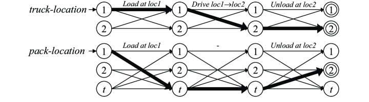
Figure 2: Logistics example broken up into two components (multi-valued state variables) that are represented by network flow problems.

1.2 The Component Solutions

We let the component solutions represent a path of value transitions in the state variables. In the networks, nodes and arcs appear in layers. Each layer represents a plan period in which, depending on the structure of the network, one or more value transitions can occur. The networks in Figures 1 and 2 each have three layers (i.e. plan periods) and their structure allows values to persist or change exactly once per period. The layers are used to solve the planning problem incrementally. That is, we start with one layer in each network and try to solve the planning problem. If no plan is found, all networks are extended by one extra layer and a new attempt is made to solve the planning problem. This process is repeated until a plan is found or a time limit is reached. In Figures 1 and 2, a path (i.e. a solution) from the source node to one of the sink nodes is highlighted in each network. Since the execution of an action triggers value transitions in the state variables, each path in a network corresponds to a sequence of actions. Consequently, the planning problem can be thought of as a collection of network flow problems where the problem is to find a path (i.e. a sequence of actions) in each of the networks. However, interactions between the networks impose side constraints on the network flow problems, which complicate the solution process.

1.3 The Merging Process

We solve these loosely coupled networks using integer programming formulations. One design choice we make is that we expand all networks (i.e. components) together, so the cost of finding solutions for the individual networks as well as merging them depends on the difficulty of solving the integer programming formulation. This, in turn, typically depends on the size of the integer programming formulation, which is partly determined by the number of layers in each of the networks. The simplest idea is to have the number of layers of the networks equal the length of the plan, just as in sequential planning where the plan length equals the number of actions in the plan. In this case, there will be as many transitions in the networks as there are actions in the plan, with the only difference that a sequence of actions corresponding to a path in a network could contain no-op actions.

An idea to reduce the required number of layers is by allowing multiple actions to be executed in the same plan period. This is exactly what is done in Graphplan (?) and in other planners that have adopted the Graphplan-style definition of parallelism. That is, two actions can be executed in parallel (i.e. in the same plan period) as long as they are non-interfering. In our formulations we adopt more general notions of parallelism. In particular, we relax the strict relation between the number of layers in the networks and the length of the plan by changing the network representation of the state variables. For example, by allowing multiple transitions in each network per plan period we permit interfering actions to be executed in the same plan period. This, however, raises issues about how solutions to the individual networks are searched and how they are combined. When the network representations for the state variables allow multiple transitions in each network per plan period, and thus become more flexible, it becomes harder to merge the solutions into a feasible plan. Therefore, to evaluate the tradeoffs in allowing such flexible representations, we look at a variety of integer programming formulations.

We refer to the integer programming formulation that uses the network representation shown in Figures 1 and 2 as the one state change model, because it allows at most one transition (i.e. state change) per plan period in each state variable. Note that in this network representation a plan period mimics the Graphplan-style parallelism. That is, two actions can be executed in the same plan period if one action does not delete the precondition or add-effect of the other action. A more flexible representation in which values can change at most once and persist before and after each change we refer to as the generalized one state change model. Clearly, we can increase the number of changes that we allow in each plan period. The representations in which values can change at most twice or $k$ times, we refer to as the generalized two state change and the generalized k state change model respectively. One disadvantage with the generalized $k$ state change model is that it creates one variable for each way to do $k$ value changes, and thus introduces exponentially many variables per plan period. Therefore, another network representation that we consider allows a path of value transitions in which each value can be visited at most once per plan period. This way, we can limit the number of variables, but may introduce cycles in our networks. The integer programming formulation that uses this representation is referred to as the state change path model.

In general, by allowing multiple transitions in each network per plan period (i.e. layer), the more complex the merging process becomes. In particular, the merging process checks whether the actions in the solutions of the individual networks can be linearized into a feasible plan. In our integer programming formulations, ordering constraints ensure feasible linearizations. There may, however, be exponentially many ordering constraints when we generalize the Graphplan-style parallelism. Rather than inserting all these constraints in the integer programming formulation up front, we add them as needed using a branch-and-cut algorithm. A branch-and-cut algorithm is a branch-and-bound algorithm in which certain constraints are generated dynamically throughout the branch-and-bound tree.

We show that the performance of our integer programming (IP) formulations show new potential and are competitive with SATPLAN04 (?). This is a significant result because it forms a basis for other more sophisticated IP-based planning systems capable of handling numeric constraints and non-uniform action costs. In particular, the new potential of our IP formulations has led to their successful use in solving partial satisfaction planning problems (?). Moreover, it has initiated a new line of work in which integer and linear programming are used in heuristic state-space search for automated planning (?, ?).

The remainder of this paper is organized as follows. In Section 2 we provide a brief background on integer programming and discuss some approaches that have used integer programming to solve planning problems. In Section 3 we present a series of integer programming formulations that each adopt a different network representation. We describe how we set up these loosely coupled networks, provide the corresponding integer programming formulation, and discuss the different variables and constraints. In Section 4 we describe the branch-and-cut algorithm that is used for solving these formulations. We provide a general background on the branch-and-cut concept and show how we apply it to our formulations by means of an example. Section 5 provides experimental results to determine which characteristics in our approach have the greatest impact on performance. Related work is discussed in Section 6 and some conclusions are given in Section 7.

2 Background

Since our formulations are based on integer programming, we briefly review this technique and discuss its use in planning. A mixed integer program is represented by a linear objective function and a set of linear inequalities:

$$\min\{cx:Ax\geq b,x_{1},...,x_{p}\geq 0\text{ and integer},x_{p+1},...,x_{n}\geq 0\},$$

where $A$ is an $(m\times n)$ matrix, $c$ is an $n$-dimensional row vector, $b$ is an $m$-dimensional column vector, and $x$ an $n$-dimensional column vector of variables. If all variables are continuous ($p=0$) we have a linear program, if all variables are integer ($p=n$) we have an integer program, and if $x_{1},...,x_{p}\in\{0,1\}$ we have a mixed 0-1 program. The set $S=\{x_{1},...,x_{p}\geq 0\text{ and integer},x_{p+1},...,x_{n}\geq 0:Ax\geq b\}$ is called the feasible region, and an $n$-dimensional column vector $x$ is called a feasible solution if $x\in S$. Moreover, the function $cx$ is called the objective function, and the feasible solution $x^{*}$ is called an optimal solution if the objective function is as small as possible, that is, $cx^{*}=\min\{cx:x\in S\}$

Mixed integer programming provides a rich modeling formalism that is more general than propositional logic. Any propositional clause can be represented by one linear inequality in 0-1 variables, but a single linear inequality in 0-1 variables may require exponentially many clauses (?).

The most widely used method for solving (mixed) integer programs is by applying a branch-and-bound algorithm to the linear programming relaxation, which is much easier to solve. The linear programming (LP) relaxation is a linear program obtained from the original (mixed) integer program by relaxing the integrality constraints:

$$\min\{cx:Ax\geq b,x_{1},...,x_{n}\geq 0\}$$

Generally, the LP relaxation is solved at every node in the branch-and-bound tree, until (1) the LP relaxation gives an integer solution, (2) the LP relaxation value is inferior to the current best feasible solution, or (3) the LP relaxation is infeasible, which implies that the corresponding (mixed) integer program is infeasible.

An ideal formulation of an integer program is one for which the solution of the linear programming relaxation is integral. Even though every integer program has an ideal formulation (?), in practice it is very hard to characterize the ideal formulation as it may require an exponential number of inequalities. In problems where the ideal formulation cannot be determined, it is often desirable to find a strong formulation of the integer program. Suppose that the feasible regions $P_{1}=\{x\in R^{n}:A_{1}x\geq b_{1}\}$ and $P_{2}=\{x\in R^{n}:A_{2}x\geq b_{2}\}$ describe the linear programming relaxations of two IP formulations of a problem. Then we say that formulation for $P_{1}$ is stronger than formulation for $P_{2}$ if $P_{1}\subset P_{2}$. That is, the feasible region $P_{1}$ is subsumed by the feasible region $P_{2}$. In other words $P_{1}$ improves the quality of the linear relaxation of $P_{2}$ by removing fractional extreme points.

There exist numerous powerful software packages that solve mixed integer programs. In our experiments we make use of the commercial solver CPLEX 10.0 (?), which is currently one of the best LP/IP solvers.

The use of integer programming techniques to solve artificial intelligence planning problems has an intuitive appeal, especially given the success IP has had in solving similar types of problems. For example, IP has been used extensively for solving problems in transportation, logistics, and manufacturing. Examples include crew scheduling, vehicle routing, and production planning problems (?). One potential advantage is that IP techniques can provide a natural way to incorporate several important aspects of real-world planning problems, such as numeric constraints and objective functions involving costs and utilities.

Planning as integer programming has, nevertheless, received only limited attention. One of the first approaches is described by Bylander (?), who proposes an LP heuristic for partial order planning algorithms. While the LP heuristic helps to reduce the number of expanded nodes, the evaluation is rather time-consuming. In general, the performance of IP often depends on the structure of the problem and on how the problem is formulated. The importance of developing strong IP formulations is discussed by Vossen et al. (?), who compare two formulations for classical planning: (1) a straightforward formulation based on the conversion of the propositional representation by SATPLAN which yields only mediocre results, and (2) a less intuitive formulation based on the representation of state transitions which leads to considerable performance improvements. Several ideas that further improve formulation based on the representation of state transitions are described by Dimopoulos (?). Some of these ideas are implemented in the IP-based planner Optiplan (?). Approaches that rely on domain-specific knowledge are proposed by Bockmayr and Dimopoulos (?, ?). By exploiting the structure of the planning problem these IP formulations often provide encouraging results. The use of LP and IP has also been explored for non-classical planning. Dimopoulos and Gerevini (?) describe an IP formulation for temporal planning and Wolfman and Weld (?) use LP formulations in combination with a satisfiability-based planner to solve resource planning problems. Kautz and Walser (?) also solve resource planning problems, but use domain-specific IP formulations.

3 Formulations

This section describes four IP formulations that model the planning problem as a collection of loosely coupled network flow problems. Each network represents a state variable, in which the nodes correspond to the state variable values, and the arcs correspond to the value transitions. The state variables are based on the SAS+ planning formalism (?), which is a planning formalism that uses multi-valued state variables instead of binary-valued atoms. An action in SAS+ is modeled by its pre-, post- and prevail-conditions. The pre- and post-conditions express which state variables are changed and what values they must have before and after the execution of the action, and the prevail-conditions specify which of the unchanged variables must have some specific value before and during the execution of an action. A SAS+ planning problem is described by a tuple $\Pi=\langle C,A,s_{0},s_{*}\rangle$ where:

• $C=\{c_{1},...,c_{n}\}$ is a finite set of state variables, where each state variable $c\in C$ has an associated domain $V_{c}$ and an implicitly defined extended domain $V^{+}_{c}=V_{c}\cup\{u\}$, where $u$ denotes the undefined value. For each state variable $c\in C$, $s[c]$ denotes the value of $c$ in state $s$. The value of $c$ is said to be defined in state $s$ if and only if $s[c]\neq u$. The total state space $S=V_{c_{1}}\times...\times V_{c_{n}}$ and the partial state space $S^{+}=V^{+}_{c_{1}}\times...\times V^{+}_{c_{n}}$ are implicitly defined.

• $A$ is a finite set of actions of the form $\langle pre,post,prev\rangle$, where $pre$ denotes the pre-conditions, $post$ denotes the post-conditions, and $prev$ denotes the prevail-conditions. For each action $a\in A$, $pre[c],post[c]$ and $prev[c]$ denotes the respective conditions on state variable $c$. The following two restrictions are imposed on all actions: (1) Once the value of a state variable is defined, it can never become undefined. Hence, for all $c\in C$, if $pre[c]\neq u$ then $pre[c]\neq post[c]\neq u$; (2) A prevail- and post-condition of an action can never define a value on the same state variable. Hence, for all $c\in C$, either $post[c]=u$ or $prev[c]=u$ or both.

• $s_{0}\in S$ denotes the initial state and $s_{*}\in S^{+}$ denotes the goal state. While SAS+ planning allows the initial state and goal state to be both partial states, we assume that $s_{0}$ is a total state and $s_{*}$ is a partial state. We say that state $s$ is satisfied by state $t$ if and only if for all $c\in C$ we have $s[c]=u$ or $s[c]=t[c]$. This implies that if $s_{*}[c]=u$ for state variable $c$, then any defined value $f\in V_{c}$ satisfies the goal for $c$.

To obtain a SAS+ description of the planning problem we use the translator component of the Fast Downward planner (?). The translator is a stand-alone component that contains a general purpose algorithm which transforms a propositional description of the planning problem into a SAS+ description. The algorithm provides an efficient grounding that minimizes the state description length and is based on the preprocessing algorithm of the MIPS planner (?).

In the remainder of this section we introduce some notation and describe our IP formulations. The formulations are presented in such a way that they progressively generalize the Graphplan-style parallelism through the incorporation of more flexible network representations. For each formulation we will describe the underlying network, and define the variables and constraints. We will not concentrate on the objective function as much because the constraints will tolerate only feasible plans.

3.1 Notation

For the formulations that are described in this paper we assume that the following information is given:

• $C$: a set of state variables;

• $V_{c}$: a set of possible values (i.e. domain) for each state variable $c\in C$;

• $E_{c}$: a set of possible value transitions for each state variable $c\in C$;

• $G_{c}=(V_{c},E_{c})$ : a directed domain transition graph for every $c\in C$;

State variables can be represented by a domain transition graph, where the nodes correspond to the possible values, and the arcs correspond to the possible value transitions. An example of the domain transition graph of a variable is given in Figure 3. While the example depicts a complete graph, a domain transition graph does not need to be a complete graph.

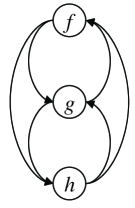
Figure 3: An example of a domain transition graph, where $V_{c}=\{f,g,h\}$ are the possible values (states) of $c$ and $E_{c}=\{(f,g),(f,h),(g,f),(g,h),(h,f),(h,g)\}$ are the possible value transitions in $c$.

Furthermore, we assume as given:

• $E^{a}_{c}\subseteq E_{c}$ represents the effect of action $a$ in $c$;

• $V^{a}_{c}\subseteq V_{c}$ represents the prevail condition of action $a$ in $c$;

• $A^{E}_{c}:=\{a\in A:|E^{a}_{c}|>0$} represents the actions that have an effect in $c$, and $A^{E}_{c}(e)$ represents the actions that have the effect $e$ in $c$;

• $A^{V}_{c}:=\{a\in A:|V^{a}_{c}|>0$} represents the actions that have a prevail condition in $c$, and $A^{V}_{c}(f)$ represents the actions that have the prevail condition $f$ in $c$;

• $C^{a}:=\{c\in C:a\in A^{E}_{c}\cup A^{V}_{c}$} represents the state variables on which action $a$ has an effect or a prevail condition.

Hence, each action is defined by its effects (i.e. pre- and post-conditions) and its prevail conditions. In SAS+ planning, actions can have at most one effect or prevail condition in each state variable. In other words, for each $a\in A$ and $c\in C$, we have that $E^{a}_{c}$ and $V^{a}_{c}$ are empty or $|E^{a}_{c}|+|V^{a}_{c}|\leq 1$. An example of how the effects and prevail conditions affect one or more domain transition graphs is given in Figure 4.

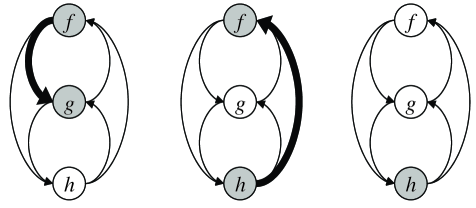
Figure 4: An example of how action effects and prevail conditions are represented in a domain transition graph. Action $a$ has implications on three state variables $C^{a}=\{c_{1},c_{2},c_{3}\}$. The effects of $a$ are represented by $E^{a}_{c_{1}}=\{(f,g)\}$ and $E^{a}_{c_{2}}=\{(h,f)\}$, and the prevail condition of $a$ is represented by $V^{a}_{c_{3}}=\{h\}$.

In addition, we use the following notation:

• $V^{+}_{c}(f)$: to denote the in-arcs of node $f$ in the domain transition graph $G_{c}$;

• $V^{-}_{c}(f)$: to denote the out-arcs of node $f$ in the domain transition graph $G_{c}$;

• $P^{+}_{c,k}(f)$: to denote paths of length $k$ in the domain transition graph $G_{c}$ that end at node $f$. Note that $P^{+}_{c,1}(f)$ = $V^{+}_{c}(f)$.

• $P^{-}_{c,k}(f)$: to denote paths of length $k$ in the domain transition graph $G_{c}$ that start at node $f$. Note that $P^{-}_{c,1}(f)$ = $V^{-}_{c}(f)$.

• $P^{\sim}_{c,k}(f)$: to denote paths of length $k$ in the domain transition graph $G_{c}$ that visit node $f$, but that do not start or end at $f$.

3.2 One State Change (1SC) Formulation

Our first IP formulation incorporates the network representation that we have seen in Figures 1 and 2. The name one state change relates to the number of transitions that we allow in each state variable per plan period. The restriction of allowing only one value transition in each network also restricts which actions we can execute in the same plan period. It happens to be the case that the network representation of the 1SC formulation incorporates the standard notion of action parallelism which is used in Graphplan (?). The idea is that actions can be executed in the same plan period as long as they do not delete the precondition or add-effect of another action. In terms of value transitions in state variables, this is saying that actions can be executed in the same plan period as long as they do not change the same state variable (i.e. there is only one value change or value persistence in each state variable).

3.2.1 State Change Network

Figure 5 shows a single layer (i.e. period) of the network which underlies the 1SC formulation. If we set up the IP formulation with $T$ plan periods, then there will be $T+1$ layers of nodes and $T$ layers of arcs in the network (the zeroth layer of nodes is for the initial state and the remaining $T$ layers of nodes and arcs are for the successive plan periods). For each possible state transition there is an arc in the state change network. The horizontal arcs correspond to the persistence of a value, and the diagonal arcs correspond to the value changes. A solution path to an individual network follows the arcs whose transitions are supported by the action effect and prevail conditions that appear in the solution plan.

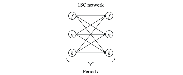
Figure 5: One state change (1SC) network.

3.2.2 Variables

We have two types of variables in this formulation: action variables to represent the execution of an action, and arc flow variables to represent the state transitions in each network. We use separate variables for changes in a state variable (the diagonal arcs in the 1SC network) and for the persistence of a value in a state variable (the horizontal arcs in the 1SC network). The variables are defined as follows:

• $x^{a}_{t}\in\{0,1\}$, for $a\in A,1\leq t\leq T$; $x^{a}_{t}$ is equal to $1$ if action $a$ is executed at plan period $t$, and $0$ otherwise.

• $\bar{y}_{c,f,t}\in\{0,1\}$, for $c\in C$, $f\in V_{c}$, $1\leq t\leq T$; $\bar{y}_{c,f,t}$ is equal to $1$ if the value $f$ of state variable $c$ persists at period $t$, and $0$ otherwise.

• $y_{c,e,t}\in\{0,1\}$, for $c\in C,e\in E_{c},1\leq t\leq T$; $y_{c,e,t}$ is equal to $1$ if the transition $e\in E_{c}$ in state variable $c$ is executed at period $t$, and $0$ otherwise.
  

3.2.3 Constraints

There are two classes of constraints. We have constraints for the network flows in each state variable network and constraints for the action effects that determine the interactions between these networks. The 1SC integer programming formulation is:

• State change flows for all $c\in C$, $f\in V_{c}$

  $$\sum_{e\in V^{-}_{c}(f)}y_{c,e,1}+\bar{y}_{c,f,1} = \left\{\begin{array}[]{ll}1\quad\textrm{if }f=s_{0}[c]\\ 0\quad\textrm{otherwise}.\end{array}\right.$$ (3)

  $$\sum_{e\in V^{-}_{c}(f)}y_{c,e,t+1}+\bar{y}_{c,f,t+1} = \sum_{e\in V^{+}_{c}(f)}y_{c,e,t}+\bar{y}_{c,f,t}\quad\text{for }1\leq t\leq T-1$$ (4)

  $$\sum_{e\in V^{+}_{c}(f)}y_{c,e,T}+\bar{y}_{c,f,T} = 1\quad\textrm{if }f=s_{*}[c]$$ (5)

• Action implications for all $c\in C$, $1\leq t\leq T$

  $$\sum_{a\in A:e\in E^{a}_{c}}x^{a}_{t} = y_{c,e,t}\quad\text{for }e\in E_{c}$$ (6)

  $$x^{a}_{t} \leq \bar{y}_{c,f,t}\quad\text{for }a\in A,f\in V^{a}_{c}$$ (7)

Constraints (3), (4), and (5) are the network flow constraints for state variable $c\in C$. Constraint (3) ensures that the path of state transitions begins in the initial state of the state variable and constraint (5) ensures that, if a goal exists, the path ends in the goal state of the state variable. Note that, if the goal value for state variable $c$ is undefined (i.e. $s_{*}[c]=u$) then the path of state transitions may end in any of the values $f\in V_{c}$. Hence, we do not need a goal constraint for the state variables whose goal states $s_{*}[c]$ are undefined. Constraint (4) is the flow conservation equation and enforces the continuity of the constructed path.

Actions may introduce interactions between the state variables. For instance, the effects of the $load$ action in our logistics example affect two different state variables. Actions link state variables to each other and these interactions are represented by the action implication constraints. For each transition $e\in E_{c}$, constraints (6) link the action execution variables that have $e$ as an effect (i.e. $e\in E^{a}_{c}$) to the arc flow variables. For example, if an action $x^{a}_{t}$ with effect $e\in E^{a}_{c}$ is executed, then the path in state variable $c$ must follow the arc represented by $y_{c,e,t}$. Likewise, if we choose to follow the arc represented by $y_{c,e,t}$, then exactly one action $x^{a}_{t}$ with $e\in E^{a}_{c}$ must be executed. The summation on the left hand side prevents two or more actions from interfering with each other, hence only one action may cause the state change $e$ in state variable $c$ at period $t$.

Prevail conditions of an action link state variables in a similar way as the action effects do. Specifically, constraint (7) states that if action $a$ is executed at period $t$ ($x^{a}_{t}=1$), then the prevail condition $f\in V^{a}_{c}$ is required in state variable $c$ at period $t$ ($\bar{y}_{c,f,t}=1$).

3.3 Generalized One State Change (G1SC) Formulation

In our second formulation we incorporate the same network representation as in the 1SC formulation, but adopt a more general interpretation of the value transitions, which leads to an unconventional notion of action parallelism. For the G1SC formulation we relax the condition that parallel actions can be arranged in any order by requiring a weaker condition. We allow actions to be executed in the same plan period as long as there exists some ordering that is feasible. More specifically, within a plan period a set of actions is feasible if (1) there exists an ordering of the actions such that all preconditions are satisfied, and (2) there is at most one state change in each of the state variables. This generalization of conditions is similar to what Rintanen, Heljanko and Niemelä (?) refer to as the $\exists$-step semantics semantics.

To illustrate the basic concept, let us again examine our small logistics example introduced in Figure 1. The solution to this problem is to load the package at location 1, drive the truck from location 1 to location 2, and unload the package at location 2. Clearly, this plan would require three plan periods under Graphplan-style parallelism as these three actions interfere with each other. If, however, we allow the $load\ at\ loc1$ and the $drive\ loc1\rightarrow loc2$ action to be executed in the same plan period, then there exists some ordering between these two actions that is feasible, namely load the package at the location 1 before driving the truck to location 2. The key idea behind this example should be clear: while it may not be possible to find a set of actions that can be linearized in any order, there may nevertheless exist some ordering of the actions that is viable. The question is, of course, how to incorporate this idea into an IP formulation.

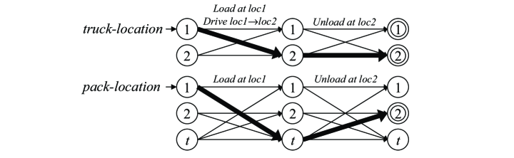
Figure 6: Logistics example represented by network flow problems with generalized arcs.

This example illustrates that we are looking for a set of constraints that allow sets of actions for which: (1) all action preconditions are met, (2) there exists an ordering of the actions at each plan period that is feasible, and (3) within each state variable, the value is changed at most once. The incorporation of these ideas only requires minor modifications to the 1SC formulation. Specifically, we need to change the action implication constraints for the prevail conditions and add a new set of constraints which we call the ordering implication constraints.

3.3.1 State Change Network

The minor modifications are revealed in the G1SC network. While the network itself is identical to the 1SC network, the interpretation of the transition arcs is somewhat different. To incorporate the new set of conditions, we implicitly allow values to persist (the dashed horizontal arcs in the G1SC network) at the tail and head of each transition arc. The interpretation of these implicit arcs is that in each plan period a value may be required as a prevail condition, then the value may change, and the new value may also be required as a prevail condition as shown in Figure 7.

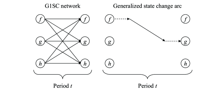
Figure 7: Generalized one state change (G1SC) network.

3.3.2 Variables

Since the G1SC network is similar to the 1SC network the same variables are used, thus, action variables to represent the execution of an action, and arc flow variables to represent the flow through each network. The difference in the interpretation of the state change arcs is dealt with in the constraints of the G1SC formulation, and therefore does not introduce any new variables. For the variable definitions, we refer to Section 3.2.2.

3.3.3 Constraints

We now have three classes of constraints, that is, constraints for the network flows in each state variable network, constraints for linking the flows with the action effects and prevail conditions, and ordering constraints to ensure that the actions in the plan can be linearized into a feasible ordering.

The network flow constraints for the G1SC formulation are identical to those in the 1SC formulation given by (3)-(5). Moreover, the constraints that link the flows with the action effects are equal to the action effect constraints in the 1SC formulation given by (6). The G1SC formulation differs from the 1SC formulation in that it relaxes the condition that parallel actions can be arranged in any order by requiring a weaker condition. This weaker condition affects the constraints that link the flows with the action prevail conditions, and introduces a new set of ordering constraints. These constraints of the G1SC formulation are given as follows:

• Action implications for all $c\in C$, $1\leq t\leq T$

  $$x^{a}_{t} \leq \bar{y}_{c,f,t}+\sum_{e\in V^{+}_{c}(f)}y_{c,e,t}+\sum_{e\in V^{-}_{c}(f)}y_{c,e,t}\quad\text{for }a\in A,f\in V^{a}_{c}$$ (8)

• Ordering implications

  $$\sum_{a\in V(\Delta)}x^{a}_{t} \leq |V(\Delta)|-1\text{ for all cycles $\Delta\in G^{prec}$ }$$ (9)

Constraint (8) incorporates this new set of conditions for which actions can be executed in the same plan period. In particular, we need to ensure that for each state variable $c$, the value $f\in V_{c}$ holds if it is required by the prevail condition of action $a$ at plan period $t$. There are three possibilities: (1) The value $f$ holds for $c$ throughout the period. (2) The value $f$ holds initially for $c$, but the value is changed to a value other than $f$ by another action. (3) The value $f$ does not hold initially for $c$, but the value is changed to $f$ by another action. In either of the three cases the value $f$ holds at some point in period $t$ so that the prevail condition for action $a$ can be satisfied. In words, the value $f$ may prevail implicitly as long as there is a state change that includes $f$. As before, the prevail implication constraints link the action prevail conditions to the corresponding network arcs.

The action implication constraints ensure that the preconditions of the actions in the plan are satisfied. This, however, does not guarantee that the actions can be linearized into a feasible order. Figure 7 indicates that there are implied orderings between actions. Actions that require the value $f$ as a prevail condition must be executed before the action that changes $f$ into $g$. Likewise, an action that changes $f$ into $g$ must be executed before actions that require the value $g$ as a prevail condition. The state change flow and action implication constraints outlined above indicate that there is an ordering between the actions, but this ordering could be cyclic and therefore infeasible. To make sure that an ordering is acyclic we start by creating a directed implied precedence graph $G^{prec}=(V^{prec},E^{prec})$. In this graph the nodes $a\in V^{prec}$ correspond to the actions, that is, $V^{prec}=A$, and we create a directed arc (i.e. an ordering) between two nodes $(a,b)\in E^{prec}$ if action $a$ has to be executed before action $b$ in time period $t$, or if $b$ has to be executed after $a$. In particular, we have

$$E^{prec} = \bigcup_{\begin{subarray}{c}(a,b)\in A\times A,c\in C,f\in V^{a}_{c},e\in E^{b}_{c}:\\ e\in V^{-}_{c,f}\end{subarray}}(a,b)\cup\bigcup_{\begin{subarray}{c}(a,b)\in A\times A,c\in C,g\in V^{b}_{c},e\in E^{a}_{c}:\\ e\in V^{+}_{c,g}\end{subarray}}(a,b)$$

The implied orderings become immediately clear from Figure 8. The figure on the left depicts the first set of orderings in the expression of $E^{prec}$. It says that the ordering between two actions $a$ and $b$ that are executed in the same plan period is implied if action $a$ requires a value to prevail that action $b$ deletes. Similarly, the figure on the right depicts second set of orderings in the expression of $E^{prec}$. That is, an ordering is implied if action $a$ adds the prevail condition of $b$.

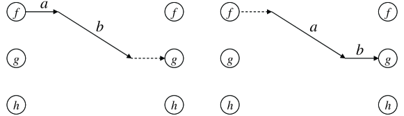
Figure 8: Implied orderings for the G1SC formulation.

The ordering implication constraints ensure that the actions in the final solution can be linearized. They basically involve putting an $n$-ary mutex relation between the actions that are involved in each cycle. Unfortunately, the number of ordering implication constraints grows exponentially in the number of actions. As a result, it will be impossible to solve the resulting formulation using standard approaches. We address this complication by implementing a branch-and-cut approach in which the ordering implication constraints are added dynamically to the formulation. This approach is discussed in Section 4.

3.4 Generalized $k$ State Change (G$k$SC) Formulation

In the G1SC formulation actions can be executed in the same plan period if (1) there exists an ordering of the actions such that all preconditions are satisfied, and (2) there occurs at most one value change in each of the state variables. One obvious generalization of this would be to relax the second condition and allow at most $k_{c}$ value changes in each state variable $c$, where $k_{c}\leq|V_{c}|-1$. By allowing multiple value changes in a state variable per plan period we, in fact, permit a series of value changes. Specifically, the G$k$SC model allows series of value changes.

Obviously, there is a tradeoff between loosening the networks versus the amount of work it takes to merge the individual plans. While we have not implemented the G$k$SC formulation, we provide some insight in this tradeoff by describing and evaluating the G$k$SC formulation with $k_{c}=2$ for all $c\in C$ We will refer to this special case as the generalized two state change (G2SC) formulation. One reason we restrict ourselves to this special case is that the general case of $k$ state changes would introduce exponentially many variables in the formulation. There are IP techniques, however, that deal with exponentially many variables (?), but we will not discuss them here.

3.4.1 State Change Network

The network that underlies the G2SC formulation is equivalent to G1SC, but spans an extra layer of nodes and arcs. This extra layer allows us to have a series of two transitions per plan period. All transitions are generalized and implicitly allow values to persist just as in the G1SC network. Figure 9 displays the network corresponding to the G2SC formulation. In the G2SC network there are generalized one and two state change arcs. For example, there is a generalized one state change arc for the transition $(f,g)$, and there is a generalized two state changes arc for the transitions $\{(f,g),(g,h)\}$. Since all arcs are generalized, each value that is visited can also be persisted. We also allow cyclic transitions, such as, $\{(f,g),(g,f)\}$ if $f$ is not the prevail condition of some action. If we were to allow cyclic transitions in which $f$ is a prevail condition of an action, then the action ordering in a plan period can not be implied anymore (i.e. the prevail condition on $f$ would either have to occur before the value transitions to $g$, or after it transitions back to $f$). Thus if there is no prevail condition on $f$ then we can safely allow the cyclic transition $\{(f,g),(g,f)\}$.

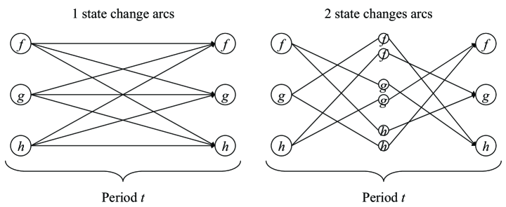
Figure 9: Generalized two state change (G2SC) network. On the left the subnetwork that consists of generalized one state change arcs and no-op arcs, on the right the subnetwork that consists of the generalized two state change arcs. The subnetwork for the two state change arcs may include cyclic transitions, such as, $\{(f,g),(g,f)\}$ as long as $f$ is not the prevail condition of some action.

3.4.2 Variables

As before we have variables representing the execution of an action, and variables representing the flows over one state change (diagonal arcs) or persistence (horizontal arcs). In addition, we have variables representing paths over two consecutive state changes. Hence, we have variables for each pair of state changes $(f,g,h)$ such that $(f,g)\in E_{c}$ and $(g,h)\in E_{c}$. We will restrict these paths to visit unique values only, that is, $f\neq g$, $g\neq h$, and $h\neq f$, or if $f$ is not a prevail condition of any action then we also allow paths where $f=h$. The variables from the G1SC formulation are also used in G2SC formulation. There is, however, an additional variable to represent the arcs that allow for two state changes:

• $y_{c,e_{1},e_{2},t}\in\{0,1\}$, for $c\in C$, $(e_{1},e_{2})\in P_{c,2}$, $1\leq t\leq T$; $y_{c,e_{1},e_{2},t}$ is equal to $1$ if there exists a value $f\in V_{c}$ and transitions $e_{1},e_{2}\in E_{c}$, such that $e_{1}\in V_{c}^{+}(f)$ and $e_{2}\in V_{c}^{-}(f)$, in state variable $c$ are executed at period $t$, and $0$ otherwise.

3.4.3 Constraints

We again have our three classes of constraints, which are given as follows:

• State change flows for all $c\in C$, $f\in V_{c}$

  $$\sum_{(e_{1},e_{2})\in P^{-}_{c,2}(f)}y_{c,e_{1},e_{2},1}+\sum_{e\in V^{-}_{c}(f)}y_{c,e,1}+\bar{y}_{c,f,1} = \left\{\begin{array}[]{ll}1\quad\textrm{if }f=s_{0}[c]\\ 0\quad\textrm{otherwise}.\end{array}\right.$$ (12)

  $$\sum_{(e_{1},e_{2})\in P^{-}_{c,2}(f)}y_{c,e_{1},e_{2},t+1}+\sum_{e\in V^{-}_{c}(f)}y_{c,e,t+1}+\bar{y}_{c,f,t+1} =$$

  $$\qquad\sum_{(e_{1},e_{2})\in P^{+}_{c,2}(f)}y_{c,e_{1},e_{2},t}+\sum_{e\in V^{+}_{c}(f)}y_{c,e,t}+\bar{y}_{c,f,t} \text{for }1\leq t\leq T-1$$ (13)

  $$\sum_{(e_{1},e_{2})\in P^{+}_{c,2}(f)}y_{c,e_{1},e_{2},T}+\sum_{e\in V^{+}_{c}(f)}y_{c,e,T}+\bar{y}_{c,f,T} = 1\quad\text{if }\{f\in s_{*}[c]\}$$ (14)

• Action implications for all $c\in C$, $1\leq t\leq T$

  $$\sum_{a\in A:e\in E^{a}_{c}}x^{a}_{t} = y_{c,e,t}+\sum_{(e_{1},e_{2})\in P_{c,2}:e_{1}=e\vee e_{2}=e}y_{c,e_{1},e_{2},t}\quad\text{for }e\in E_{c}$$ (15)

  $$x^{a}_{t} \leq \bar{y}_{c,f,t}+\sum_{e\in V^{+}_{c}(f)}y_{c,e,t}+\sum_{e\in V^{-}_{c}(f)}y_{c,e,t}+\sum_{(e_{1},e_{2})\in P^{\sim}_{c,2}(f)}y_{c,e_{1},e_{2},t}+$$ (16)

  $$\sum_{(e_{1},e_{2})\in P^{+}_{c,2}(f)}y_{c,e_{1},e_{2},t}+\sum_{(e_{1},e_{2})\in P^{-}_{c,2}(f)}y_{c,e_{1},e_{2},t}\quad\text{for }a\in A,f\in V^{a}_{c}$$

• Ordering implications

  $$\sum_{a\in V(\Delta)}x^{a}_{t} \leq |V(\Delta)|-1\text{ for all cycles $\Delta\in G^{prec}$ }$$ (17)

Constraints (12), (13), and (14) represent the flow constraints for the G2SC network. Constraints (15) and (16) link the action effects and prevail conditions with the corresponding flows, and constraint 17 ensures that the actions can be linearized into some feasible ordering.

3.5 State Change Path (PathSC) Formulation

There are several ways to generalize the network representation of the G1SC formulation and loosen the interaction between the networks. The G$k$SC formulation presented one generalization that allows up to $k$ transitions in each state variable per plan period. Since it uses exponentially many variables another way to generalize the network representation of the G1SC formulation is by requiring that each value can be true at most once per plan period. To illustrate this idea we consider our logistics example again, but we now use a network representation that allows a path of transitions per plan period as depicted in Figure 10.

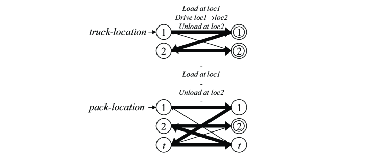
Figure 10: Logistics example represented by network flow problems that allow a path of value transitions per plan period such that each value can be true at most once.

Recall that the solution to the logistics example consists of three actions: first load the package at location 1, then drive the truck from location 1 to location 2, and last unload the package at location 2. Clearly, this solution would not be allowed within a single plan period under Graphplan-style parallelism. Moreover, it would also not be allowed within a single period in the G1SC formulation. The reason for this is that the number of value changes in the $package\text{-}location$ state variable is two. First, it changes from $pack\text{-}at\text{-}loc1$ to $pack\text{-}in\text{-}truck$, and then it changes from $pack\text{-}in\text{-}truck$ to $pack\text{-}at\text{-}loc2$. As before, however, there does exists an ordering of the three actions that is feasible. The key idea behind this example is to show that we can allow multiple value changes in a single period. If we limit the value changes in a state variable to simple paths, that is, in one period each value is visited at most once, then we can still use implied precedences to determine the ordering restrictions.

3.5.1 State Change Network

In this formulation each value can be true at most once in each plan period, hence the number of value transitions for each plan period is limited to $k_{c}$ where $k_{c}=|V_{c}|-1$ for each $c\in C$. In the PathSC network, nodes appear in layers and correspond to the values of the state variable. However, each layer now consists of twice as many nodes. If we set up an IP encoding with a maximum number of plan periods $T$ then there will be $T$ layers. Arcs within a layer correspond to transitions or to value persistence, and arcs between layers ensure that all plan periods are connected to each other.

Figure 11 displays a network corresponding to the state variable $c$ with domain $V_{c}=\{f,g,h\}$ that allows multiple transitions per plan period. The arcs pointing rightwards correspond to the persistence of a value, while the arcs pointing leftwards correspond to the value changes. If more than one plan period is needed the curved arcs pointing rightwards link the layers between two consecutive plan periods. Note that with unit capacity on the arcs, any path in the network can visit each node at most once.

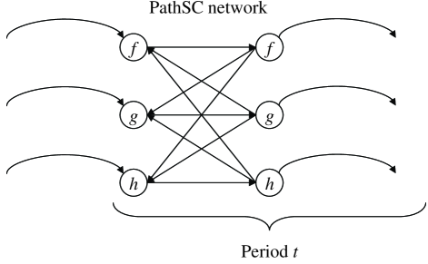
Figure 11: Path state change (PathSC) network.

3.5.2 Variables

We now have action execution variables and arc flow variables (as defined in the previous formulations), and linking variables that connect the networks between two consecutive time periods. These variables are defined as follows:

• $z_{c,f,t}\in\{0,1\}$, for $c\in C,f\in V_{c},0\leq t\leq T$; $z_{c,f,t}$ is equal to $1$ if the value $f$ of state variable $c$ is the end value at period $t$, and $0$ otherwise.

3.5.3 Constraints

As in the previous formulations, we have state change flow constraints, action implication constraints, and ordering implication constraints. The main difference is the underlying network. The PathSC integer programming formulation is given as follows:

• State change flows for all $c\in C$, $f\in V_{c}$

  $$z_{c,f,0} = \left\{\begin{array}[]{ll}1\quad\textrm{if }f=s_{0}[c]\\ 0\quad\textrm{otherwise}.\end{array}\right.$$ (20)

  $$\sum_{e\in V^{+}_{c}(f)}y_{c,e,t}+z_{c,f,t-1} = \bar{y}_{c,f,t}$$ (21)

  $$\bar{y}_{c,f,t} = \sum_{e\in V^{-}_{c}(f)}y_{c,e,t}+z_{c,f,t}\quad\text{for }1\leq t\leq T-1$$ (22)

  $$z_{c,f,T} = 1\quad\text{if }f\in s_{*}[c]$$ (23)

• Action implications for all $c\in C$, $1\leq t\leq T$

  $$\sum_{a\in A:e\in E^{a}_{c}}x^{a}_{t} = y_{c,e,t}\quad\text{for }e\in E_{c}$$ (24)

  $$x^{a}_{t} \leq \bar{y}_{c,f,t}\quad\text{for }f\in V^{a}_{c}$$ (25)

• Ordering implications

  $$\sum_{a\in V(\Delta)}x^{a}_{t} \leq |V(\Delta)|-1\text{ for all cycles }\Delta\in G^{prec^{\prime}}$$ (26)

Constraints (20)-(23) are the network flow constraints. For each node, except for the initial and goal state nodes, they ensure a balance of flow (i.e. flow-in must equal flow-out). The initial state node has a supply of one unit of flow and the goal state node has a demand of one unit of flow, which are given by constraints (20) and (23) respectively. The interactions that actions impose upon different state variables are represented by the action implication constraints (24) and (25), which have been discussed earlier.

The implied precedence graph for this formulation is given by $G^{prec^{\prime}}=(V^{prec^{\prime}},E^{prec^{\prime}})$. It has an extra set of arcs to incorporate the implied precedences that are introduced when two actions imply a state change in the same class $c\in C$. The nodes $a\in V^{prec^{\prime}}$ again correspond to actions, and there is an arc $(a,b)\in E^{prec^{\prime}}$ if action $a$ has to be executed before action $b$ in the same time period, or if $b$ has to be executed after $a$. More specifically, we have

$$E^{prec^{\prime}} = E^{prec}\cup\bigcup_{\begin{subarray}{c}(a,b)\in A\times A,c\in C,f\in V_{c},e\in E^{a}_{c},e^{\prime}\in E^{b}_{c}:\\ e\in V^{+}_{c}(f)\wedge e^{\prime}\in V^{-}_{c}(f)\end{subarray}}(a,b)$$

As before, the ordering implication constraints (26) ensure that the actions in the solution plan can be linearized into a feasible ordering.

4 Branch-and-Cut Algorithm

IP problems are usually solved with an LP-based branch-and-bound algorithm. The basic structure of this technique involves a binary enumeration tree in which branches are pruned according to bounds provided by the LP relaxation. The root node in the enumeration tree represents the LP relaxation of the original IP problem and each other node represents a subproblem that has the same objective function and constraints as the root node except for some additional bound constraints. Most IP solvers use an LP-based branch-and-bound algorithm in combination with various preprocessing and probing techniques. In the last few years there has been significant improvement in the performance of these solvers (?).

In an LP-based branch-and-bound algorithm, the LP relaxation of the original IP problem (the solution to the root node) will rarely be integer. When some integer variable $x$ has a fractional solution $v$ we branch to create two new subproblems, such that the bound constraint $x\leq\lfloor v\rfloor$ is added to the left-child node, and $x\geq\lceil v\rceil$ is added to the right-child node. This branching process is carried out recursively to expand those subproblems whose solution remains fractional. Eventually, after enough bounds are placed on the variables, an integer solution is found. The value of the best integer solution found so far, $Z^{*}$, is referred to as the incumbent and is used for pruning.

In a minimization problem, branches emanating from nodes whose solution value $Z_{\text{LP}}$ is greater than the current incumbent, $Z^{*}$, can never give rise to a better integer solution as each child node has a smaller feasible region than its parent. Hence, we can safely eliminate such nodes from further consideration and prune them. Nodes whose feasible region have been reduced to the empty set, because too many bounds are placed on the variables, can be pruned as well.

When solving an IP problem with an LP-based branch-and-bound algorithm we must consider the following two decisions. If several integer variables have a fractional solution, which variable should we branch on next, and if the branch we are currently working on is pruned, which subproblem should we solve next? Basic rules include use the “most fractional variable” rule for branching variable selection and the “best objective value” rule for node selection.

For our formulations a standard LP-based branch-and-bound algorithm approach is very ineffective due to the large number (potentially exponentially many) ordering implication constraints in the G1SC, G2SC, and PathSC formulations. While it is possible to reduce the number of constraints by introducing additional variables (?), the resulting formulations would still be intractable for all but the smallest problem instances. Therefore, we solve the IP formulations with a so-called branch-and-cut algorithm, which considers the ordering implication constraints implicitly. A branch-and-cut algorithm is a branch-and-bound algorithm in which certain constraints are generated dynamically throughout the branch-and-bound tree. A flowchart of our branch-and-cut algorithm is given in Figure 12.

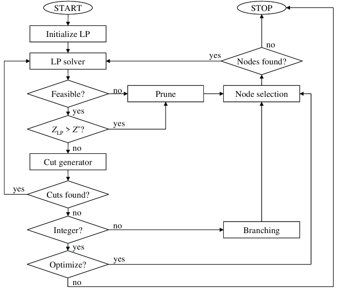
Figure 12: Flowchart of our branch-and-cut algorithm. For finding any feasible solution (i.e. optimize = no) the algorithm stops as soon as the first feasible integer solution is found. When searching for the optimal solution (i.e. optimize = yes) for the given formulation we continue until no open nodes are left.

If, after solving the LP relaxation, we are unable to prune the node on the basis of the LP solution, the branch-and-cut algorithm tries to find a violated cut, that is, a constraint that is valid but not satisfied by the current solution. This is also known as the separation problem. If one or more violated cuts are found, the constraints are added to the formulation and the LP is solved again. If none are found, the algorithm creates a branch in the enumeration tree (if the solution to the current subproblem is fractional) or generates a feasible solution (if the solution to the current subproblem is integral).

The basic idea of branch-and-cut is to leave out constraints from the LP relaxation of which there are too many to handle efficiently, and add them to the formulation only when they become binding at the solution to the current LP. Branch-and-cut algorithms have successfully been applied in solving hard large-scale optimization problems in a wide variety of applications including scheduling, routing, graph partitioning, network design, and facility location problems (?).

In our branch-and-cut algorithm we can stop as soon as we find the first feasible solution, or we can implicitly enumerate all nodes (through pruning) and find the optimal solution for a given objective function. Note that our formulations can only be used to find bounded length optimal plans. That is, find the optimal plan given a plan period (i.e. a bounded length). In our experimental results, however, we focus on finding feasible solutions.

4.1 Constraint Generation

At any point during runtime that the cut generator is called we have a solution to the current LP problem, which consists of the LP relaxation of the original IP problem plus any added bound constraints and added cuts. In our implementation of the branch-and-cut algorithm, we start with an LP relaxation in which the ordering implication constraints are omitted. So given a solution to the current LP relaxation, which could be fractional, the separation problem is to determine whether the solution violates one of the omitted ordering implication constraints. If so, we identify the violated ordering implication constraints, add them to the formulation, and resolve the new problem.

4.1.1 Cycle Identification

In the G1SC, G2SC, and PathSC formulations an ordering implication constraint is violated if there is a cycle in the implied precedence graph. Separation problems involving cycles occur in numerous applications. Probably the best known of its kind is the traveling salesman problem in which subtours (i.e. cycles) are identified and subtour elimination constraints are added to the current LP. Our algorithm for separating cycles is based on the one described by Padberg and Rinaldi (?). We are interested in finding the shortest cycle in the implied precedence graph, as the shortest cycle cuts off more fractional extreme points. The general idea behind this approach is as follows:

1. Given a solution to the LP relaxation, determine the subgraph $G_{t}$ for plan period $t$ consisting of all the nodes $a$ for which $x^{a}_{t}>0$.

2. For all the arcs $(a,b)\in G_{t}$, define the weights $w_{a,b}:=x^{a}_{t}+x^{b}_{t}-1$.

3. Determine the shortest path distance $d_{a,b}$ for all pairs ($(a,b)\in G_{t}$) based on arc weights $\bar{w}_{a,b}:=1-w_{a,b}$ (for example, using the Floyd-Warshall all-pairs shortest path algorithm).

4. If $d_{a,b}-w_{b,a}<0$ for some arc $(a,b)\in G_{t}$, there exists a violated cycle constraint.

While the general principles behind branch-and-cut algorithms are rather straightforward, there are a number of algorithmic and implementation issues that may have a significant impact on overall performance. At the heart of these issues is the trade-off between computation time spent at each node in the enumeration tree and the number of nodes that are explored. One issue, for example, is to decide when to generate violated cuts. Another issue is which of the generated cuts (if any) should be added to the LP relaxation, and whether and when to delete constraints that were added to the LP before. In our implementation, we have only addressed these issues in a straightforward manner: cuts are generated at every node in the enumeration tree, the first cut found by the algorithm is added, and constraints are never deleted from the LP relaxation. However, given the potential of more advanced strategies that has been observed in other applications, we believe there still may be considerable room for improvement.

4.1.2 Example

In this section we will show the workings of our branch-and-cut algorithm on the G1SC formulation using a small hypothetical example involving two state variables $c_{1}$ and $c_{2}$, five actions $A1$, $A2$, $A3$, $A4$, and $A5$, and one plan period. In particular we will show how the cycle detection procedure works and how an ordering implication constraint is generated.

Figure 13 depicts a solution to the current LP of the planning problem. For state variable $c_{1}$ we have that actions $A1$ and $A2$ have a prevail condition on $g$, $A4$ has a prevail condition on $h$, and action $A3$ has an effect that changes $g$ into $h$. Likewise, for state variable $c_{2}$ we have that action $A4$ has an effect that changes $g$ into $f$, action $A5$ changes $g$ into $h$, and action $A1$ has a prevail condition on $f$. Note that the given solution is fractional. Therefore some of the action variables have fractional values. In particular, we have $x^{A1}=x^{A4}=0.8$, $x^{A5}=0.2$, and $x^{A2}=x^{A3}=1$. In other words, actions $A2$ and $A3$ are fully executed while actions $A1$, $A4$ and $A5$ are only fractionally executed. Clearly, in automated planning the fractional execution of an action has no meaning whatsoever, but it is very common that the LP relaxation of an IP formulation gives a fractional solution. We simply try to show that we can find a violated cut even when we have a fractional solution. Also, note that the actions $A4$ and $A5$ have interfering effects in $c_{2}$. While this would generally be infeasible, the actions are executed only fractionally, so this is actually a feasible solution to the LP relaxation of the IP formulation.

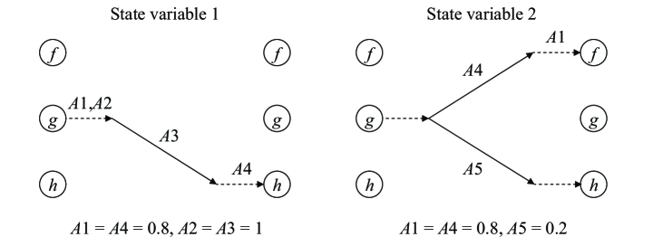
Figure 13: Solution to a small hypothetical planning example. The solution to the current LP has flows over the indicated paths and executes actions $A1$, $A2$, $A3$, $A4$, and $A5$.

In order to determine whether the actions can be linearized into a feasible ordering we first create the implied precedence graph $G^{prec}=(V^{prec},E^{prec})$, where we have $V^{prec}=\{A1,A2,A3,A4,A5\}$ and $E^{prec}=$ $\{(A1,A3)$,$(A2,A3)$,$(A3,A4)$,$(A4,A1)\}$. The ordering $(A1,A3)$, for example, is established by the effects of these actions in state variable $c_{1}$. $A1$ has a prevail condition $g$ in $c_{1}$ while $A3$ changes $g$ to $h$ in $c_{1}$, which implies that $A1$ must be executed before $A3$. The other orderings are established in a similar way. The complete implied precedence graph for this example is given in Figure 14.

The cycle detection algorithm gets the implied precedence graph and the solution to the current LP as input. Weights for each arc $(a,b)\in E^{prec}$ are determined by the values of the action variables in the current solution. We have the LP solution that is given in Figure 13, so in this example we have $w_{A1,A3}=w_{A3,A4}=0.8$, $w_{A2,A3}=1$, and $w_{A4,A1}=0.6$. The length of the shortest path from $A1$ to $A4$ using weights $\bar{w}_{a,b}$ is equal to $0.4$ $(0.2+0.2)$. Hence, we have $d_{A1,A4}=0.4$ and $w_{A4,A1}=0.6$. Since $d_{A1,A4}-w_{A4,A1}<0$, we have a violated cycle (i.e. violated ordering implication) that includes all actions that are on the shortest path from $A1$ to $A4$ (i.e. $A1$, $A3$, and $A4$, which can be retrieved by the shortest path algorithm). This generates the following ordering implication constraint $x^{A1}_{1}+x^{A3}_{1}+x^{A4}_{1}\leq 2$, which will be added to the current LP. Note that this ordering constraint is violated by the current LP solution, as $x^{A1}_{1}+x^{A3}_{1}+x^{A4}_{1}=0.8+1+0.8=2.6$. Once the constraint is added to the LP, the next solution will select a set of actions that does not violate the newly added cut. This procedure continues until no cuts are violated and the solution is integer.

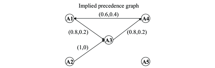
Figure 14: Implied precedence graph for this example, where the labels show $(w_{a,b},\bar{w}_{a,b})$.

5 Experimental Results

The described formulations are based on two key ideas. The first idea is to decompose the planning problem into several loosely coupled components and represent these components by an appropriately defined network. The second idea is to reduce the number of plan periods by adopting different notions of parallelism and use a branch-and-cut algorithm to dynamically add constraints to the formulation in order to deal with the exponentially many action ordering constraints in an efficient manner.

To evaluate the tradeoffs of allowing more flexible network representations we compare the performance of the one state change (1SC) formulation, the generalized one state change formulation (G1SC), the generalized two state change (G2SC) formulation, and the state change path (PathSC) formulation. For easy reference, an overview of these formulations is given in Figure 15.

In our experiments we focus on finding feasible solutions. Note, however, that our formulations can be used to do bounded length optimal planning. That is, given a plan period (i.e. a bounded length), find the optimal solution.

1SC	G1SC
Each state variable can change or	Each state variable can change (and
prevail a value at most once per	prevail a value before and after each
plan period.	change) at most once per plan period.
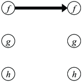
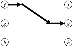
G2SC	PathSC
Each state variable can change (and	The state variable can change any
prevail a value before and after each	number of times, but each value
change) at most twice per plan	can be true at most once per plan
period. Cyclic changes $(f,g,f)$ are	period.
allowed only if $f$ is not the
prevail condition of some action

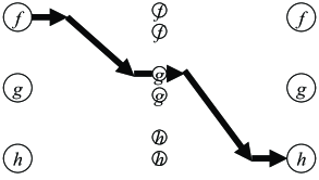
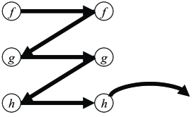
Figure 15: Overview of the 1SC, G1SC, G2SC, and PathSC formulations.

5.1 Experimental Setup

To compare and analyze our formulations we use the STRIPS domains from the second and third international planning competitions (IPC2 and IPC3 respectively). That is, Blocksworld, Logistics, Miconic, Freecell from IPC2 and Depots, Driverlog, Zenotravel, Rovers, Satellite, and Freecell from IPC3. We do not compare our formulations on the STRIPS domains from IPC4 and IPC5 mainly because of a peripheral limitation of the current implementation of the G2SC and PathSC formulations. In particular, the G2SC formulation cannot handle operators that change a state variable from an undefined value to a defined value, and the PathSC formulation cannot handle such operators if the domain size of the state variable is larger than two. Because of these limitations we could not test the G2SC formulation on the Miconic, Satellite and Rovers domains, and we could not test the PathSC formulation on the Satellite domain.

In order to setup our formulations we translate a STRIPS planning problem into a multi-valued state description using the translator of the Fast Downward planner (?). Each formulation uses its own network representation and starts by setting the number of plan periods $T$ equal to one. We try to solve this initial formulation and if no plan is found, $T$ is increased by one, and then try to solve this new formulation. Hence, the IP formulation is solved repeatedly until the first feasible plan is found or a 30 minute time limit (the same time limit that is used in the international planning competitions) is reached. We use CPLEX 10.0 (?), a commercial LP/IP solver, for solving the IP formulations on a 2.67GHz Linux machine with 1GB of memory.

We set up our experiments as follows. First, in Section 5.2 we provide a brief overview of our main results by looking at aggregated results from IPC2 and IPC3. Second, in Section 5.3, we give a more detailed analysis on our loosely coupled encodings for planning and focus on the tradeoffs of reducing the number of plan periods to solve a planning problem versus the increased difficulty in merging the solutions to the different components. Third, in Section 5.4 we briefly touch upon how different state variable representations of the same planning problem can influence performance.

5.2 Results Overview

In this general overview we compare our formulations to the following planning systems: Optiplan (?), SATPLAN04 (?), SATPLAN06 (?), and Satplanner (?).

Optiplan is an integer programming based planner that participated in the optimal track of the fourth international planning competition. Like our formulations, Optiplan models state transitions but it does not use a factored representation of the planning domain. In particular, Optiplan represents state transitions in the atoms of the planning domain, whereas our formulations use multi-valued state variables. Apart from this, Optiplan is very similar to the 1SC formulation as they both adopt the Graphplan-style parallelism.

SATPLAN04, SATPLAN06, and Satplanner are satisfiability based planners. SATPLAN04 and SATPLAN06 are versions of the well known system SATPLAN (?), which has a long track record in the international planning competitions. Satplanner has not received that much attention, but is among the state-of-the-art in planning as satisfiability. Like our formulations Satplanner generalizes the Graphplan-style parallelism to improve planning efficiency.

The main results are summarized by Figure 16. It displays aggregate results from IPC2 and IPC3, where the number of instances solved (y-axis) is drawn as a function of log time (x-axis). We must note that the graph with the IPC2 results favors the PathSC formulation over all other planners. However, as we will see in Section 5.3, this is mainly a reflection of its exceptional performance in the Miconic domain rather than its overall performance in IPC2. Morever, the graph with the IPC3 results does not include the Satellite domain. We decided to remove this domain, because we could not run it on the public versions of SATPLAN04 and SATPLAN06 nor the G2SC and PathSC formulations. While the results in Figure 16 provide a rather coarse overview, they sum up the following main findings.

• Factored planning using loosely coupled formulations helps improve performance. Note that all integer programming formulations that use factored representations, that is 1SC, G1SC, G2SC, and PathSC (except the G2SC formulation which could not be tested on all domains), are able to solve more problem instances in a given amount of time than Optiplan, which does not use a factored representation. Especially, the difference between 1SC and Optiplan is remarkable as they both adopt the Graphplan-style parallelism. In Section 5.3, however, we will see that Optiplan does perform well in domains that are either serial by design or have a significant serial component.

• Decreasing the encoding size by relaxing the Graphplan-style parallelism helps improve performance. This is not too surprising, Dimopoulos et al. (?) already note that a reduction in the number of plan periods helps improve planning performance. However, this does not always hold because of the tradeoff between reducing the number plan periods versus the increased difficulty in merging the solutions to the different components. In Section 5.3 we will see that different relaxations of Graphplan-style parallelism lead to different results. For example, the PathSC formulation shows superior performance in Miconic and Driverlog, but does poorly in Blocksworld, Freecell, and Zenotravel. Likewise, the G2SC formulation does well in Freecell, but it does not seem to excel in any other domain.

• Planning as integer programming shows new potential. The conventional wisdom in the planning community has been that planning as integer programming cannot compete with planning as satisfiability or constraint satisfaction. In Figure 16, however, we see that the 1SC, G1SC and PathSC formulation can compete quite well with SATPLAN04. While SATPLAN04 is not state-of-the-art in planning as satisfiability anymore, it does show that planning as integer programming has come a long way. The fact that IP is competitive allows us to exploit its other virtues such as optimization (?, ?, ?).

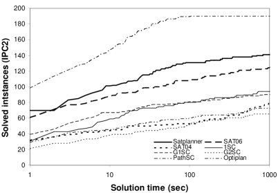
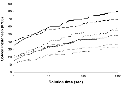
Figure 16: Aggregate results of the second and third international planning competitions.

5.3 Comparing Loosely Coupled Formulations for Planning

In this section we compare our IP formulations and try to evaluate the benefits of allowing more flexible network representations. Specifically, we are interested in the effects of reducing the number of plan periods required to solve the planning problem versus dealing with merging solutions to the different components. Reducing the number of plan periods can lead to smaller encodings, which can lead to improved performance. However, it also makes the merging of the loosely coupled components harder, which could worsen performance.

In order to compare our formulations we will analyze the following two things. First, we examine the performance of our formulations by comparing their solution times on problem instances from IPC2 and IPC3. In this comparison we will include results from Optiplan as it gives us an idea of the differences between a formulation based on Graphplan and formulations based on loosely coupled components. Moreover, it will also show us the improvements in IP based approaches for planning. Second, we examine the number of plan periods that each formulation needs to solve each problem instance. Also, we will look at the tradeoffs between reducing the number of plan periods and the increased difficulty in merging the solutions of the loosely coupled components. In this comparison we will include results from Satplanner because, just like our formulations, it adopts a generalized notion of the Graphplan-style parallelism.

We use the following figures and table. Figure 17 shows the total solution time (y-axis) needed to solve the problem instances (x-axis), Figure 18 shows the number of plan periods (y-axis) to solve the problem instances (x-axis), and Table 1 shows the number of ordering constraints that were added during the solution process, which can be seen as an indicator of the merging effort. The selected problem instances in Table 1 represent the five largest instances that could be solved by all of our formulations (in some domains, however, not all formulations could solve at least five problem instances).

The label $GPsteps$ in Figure 18 represents the number of plan steps that SATPLAN06, a state-of-the-art Graphplan-based planner, would use. In the Satellite domain, however, we use the results from the 1SC formulation as we were unable to run the public version of SATPLAN06 in this domain. We like to point out that Figure 18 is not intended to favor one formulation over the other, it simply shows that it is possible to generate encodings for automated planning that use drastically fewer plan periods than Graphplan-based encodings.

5.3.1 Results: Planning Performance

Blocksworld is the only domain in which Optiplan solves more problems than our formulations. In Zenotravel and Satellite, Optiplan is generally outperformed with respect to solution time, and in Rovers and Freecell, Optiplan is generally outperformed with respect to the number of problems solved. As for the other IP formulations, the G1SC provides the overall best performance and the performance of the PathSC formulation is somewhat irregular. For example, in Miconic, Driverlog and Rovers the PathSC formulation does very well, but in Depots and Freecell it does rather poorly.

In the Logistics domain all formulations that generalize the Graphplan-style parallelism (i.e. G1SC, G2SC, and PathSC) scale better than the 1SC formulation and Optiplan, which adopt the Graphplan-style parallelism. Among G1SC, G2SC, and PathSC formulations there is no clear best performer, but in the larger Logistics problems the G1SC formulation seems to do slightly better. The Logistics domain provides a great example of the tradeoff between flexibility and merging. By allowing more actions to be executed in each plan period, generally shorter plans (in terms of number of plan periods) are needed to solve the planning problem (see Figure 18), but at the same time merging the solutions to the individual components will be harder as one has to respect more ordering constraints (see Table 1).

Optiplan versus 1SC. If we compare the 1SC formulation with Optiplan, we note that Optiplan fares well in domains that are either serial by design (Blocksworld) or in domains that have a significant serial aspect (Depots). We think that Optiplan’s advantage over the 1SC formulation in these domains is due to the following two possibilities. First, our intuition is that in serial domains the reachability and relevance analysis in Graphplan is stronger in detecting infeasible action choices (due to mutex propagation) than the network flow restrictions in the 1SC formulation. Second, it appears that the state variables in these domains are more tightly coupled (i.e. the actions have more effects, thus transitions in one state variable are coupled with several transitions in other state variables) than in most other domains, which may negatively affect the performance of the 1SC formulation.

1SC versus G1SC. When comparing the 1SC formulation with the G1SC formulation we can see that in all domains, except in Blocksworld and Miconic, the G1SC formulation solves at least as many problems as the 1SC formulation. The results in Blocksworld are not too surprising and can be attributed to semantics of this domain. Each operator in Blocksworld requires one state change in the state variable of the arm ($stack$ and $putdown$ change the status of the arm to $arm-empty$, and $unstack$ and $pickup$ change the status of the arm to $holding-x$ where $x$ is the block being lifted). Since, the 1SC and the G1SC formulations both allow at most one state change in each state variable, there is no possibility for the G1SC formulation to allow more than one action to be executed in the same plan period. Given this, one may think that the 1SC and G1SC formulations should solve at least the same number of problems, but in this case the prevail constraints (7) of the 1SC formulation are stronger than the prevail constraints (8) of the G1SC formulation. That is, the right-hand side of (8) subsumes (i.e. allows for a larger feasible region in the LP relaxation) than the right-hand side of (7). In Figure 17 we can see this slight advantage of 1SC over G1SC in the Blocksworld domain.

The results in the Miconic domain are, on the other hand, not very intuitive. We would have expected the G1SC formulation to solve at least as many problems as the 1SC formulation, but this did not turn out to be the case. One thing we noticed is that in this domain the G1SC formulation required a lot more time to determine that there is no plan for a given number of plan periods.

G1SC versus G2SC and PathSC. Table 1 only shows the five largest problems in each domain that were solved by the formulations, yet it is representative for the whole set of problems. The table indicates that when Graphplan-style parallelism is generalized, more ordering constraints are needed to ensure a feasible plan. On average, the G2SC formulation includes more ordering constraints than the G1SC formulation, and the PathSC formulation in its turn includes more ordering constraints than the G2SC formulation. The performance of these formulations as shown by Figure 17 varies per planning domain. The PathSC formulation does well in Miconic and Driverlog, the G2SC formulation does well in Freecell, and the G1SC does well in Zenotravel. Because of these performance differences, we believe that the ideal amount of flexibility in the generalization of Graphplan-style parallelism is different for each planning domain.

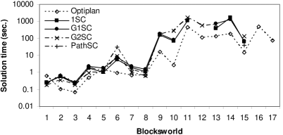
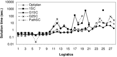
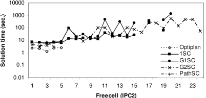
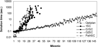
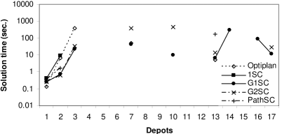
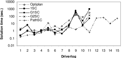
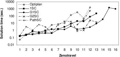
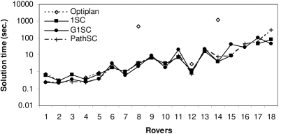
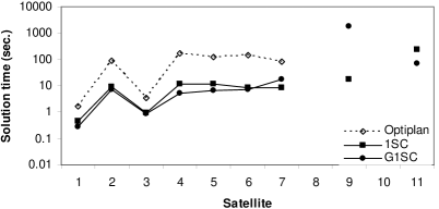
Figure 17: Solution times in the planning domains of the second and third international planning competition.

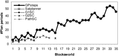
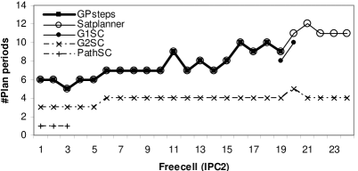
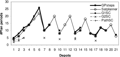
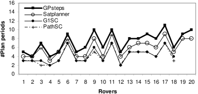
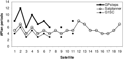
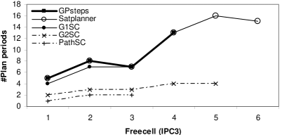
Figure 18: Number of plan periods required for each formulation to solve the planning problems in the second and third international planning competition.

Problem G1SC G2SC PathSC Blocksworld 5-1 0 0 16 5-2 0 0 62 6-0 0 0 5 6-1 0 0 5 8-2 0 0 62 Logistics 10-1 0 7 11 11-0 0 0 10 11-1 0 0 49 12-0 0 16 9 14-0 0 7 110 Freecell 2-1 0 0 0 2-2 0 0 0 2-3 0 0 84 2-4 0 2 0 5-5 0 3 * Miconic 6-4 0 - 0 7-0 0 - 0 7-2 0 - 2 7-3 0 - 4 9-4 0 - 5

Problem G1SC G2SC PathSC Depots 1 0 0 7 2 0 0 2 10 0 2 * 13 0 0 30 17 0 0 * Driverlog 7 1 16 2 8 32 62 108 9 58 80 32 10 5 5 69 11 6 30 11 Zenotravel 5 0 4 485 6 0 5 6 10 0 0 214 11 0 0 586 12 0 60 6259 Rovers 14 0 - 13 15 12 - 11 16 1 - 92 17 1 - 4 18 1 - 192 Satellite 5 2 - - 6 6 - - 7 8 - - 9 14 - - 11 0 - - Freecell 1 0 0 3 2 0 0 2480 3 0 1 1989 4 * 1 * 5 * 0 *

Table 1: Number of ordering constraints, or cuts, that were added dynamically through the solution process to problems in IPC2 (left) and IPC3 (right). A dash ‘-’ indicates that the IP formulation could not be tested on the domain and a star ‘*’ indicates that the formulation could not solve the problem instance within 30 minutes.

5.3.2 Results: Number of Plan Periods

In Figure 18, we see that in all domains the flexible network representation of the G1SC formulation is slightly more general than the 1-linearization semantics that is used by Satplanner. That is, the number of plan periods required by the G1SC formulation is always less than or equal to the number of plan periods used by Satplanner. Moreover, the flexible network representation of the G2SC and PathSC formulations are both more general than the one used by the G1SC formulation. One may think that the network representation of the PathSC formulation should provide the most general interpretation of action parallelism, but since the G2SC network representations allows some values to change back to their original value in the same plan period this is not always the case.

In the domains of Logistics, Freecell, Miconic, and Driverlog, the PathSC never required more than two plan periods to solve the problem instances. For the Miconic domain this is very easy to understand. In Miconic there is an elevator that needs to bring travelers from one floor to another. The state variables representation of this domain has one state variable for the elevator and two for each traveler (one to represent whether the traveler has boarded the elevator and one to represent whether the traveler has been serviced). Clearly, one can devise a plan such that each value of the state variable is visited at most twice. The elevator simply could visit all floors and pickup all the travelers, and then visit all floors again to bring them to their destination floor.

5.4 Comparing Different State Variable Representations

An interesting question is to find out whether different state variable representations lead to different performance benefits. In our loosely coupled formulations we have components that represent multi-valued state variables. However, the idea of modeling value transitions as flows in an appropriately defined network can be applied to any binary or multi-valued state variable representation. In this section we concentrate on the efficiency tradeoffs between binary and multi-valued state descriptions. As there are generally fewer multi-valued state variables than binary atoms needed to describe a planning problem, we can expect our formulations to be more compact when they use a multi-valued state description. For this comparison we only concentrate on the G1SC formulation as it showed the overall best performance among our formulations. In our recent work (?) we analyze different state variable representations in more detail.

Table 2 compares the encoding size for the G1SC formulation on a set of problems using either a binary or multi-valued state description. The table clearly shows that the encoding size becomes significantly smaller (both before and after CPLEX presolve) when a multi-valued state description is used. The encoding size before presolve gives an idea of the impact of using a more compact multi-valued state description, whereas the encoding size after presolve shows how much preprocessing can be done by removing redundancies and substituting out variables.

Figure 19 shows the total solution time (y-axis) needed to solve the problem instances (x-axis). Since we did not make any changes to the G1SC formulation, the performance differences are the result of using different state descriptions. In several domains the multi-valued state description shows a clear advantage over the binary state description when using the G1SC formulation, but there are also domains in which the multi-valued state description does not provide too much of an advantage. In general, however, the G1SC formulation using a multi-valued state description leads to the same or better performance than using a binary state description. In all our tests, we encountered only one problem instance (Rovers pfile10) in which the binary state description notably outperformed the multi-valued state description.

	Binary				Multi
	Before presolve		After presolve		Before presolve		After presolve
Problem	#va	#co	#va	#co	#va	#co	#va	#co
Blocksworld
6-2	7645	12561	5784	9564	5125	7281	3716	5409
7-0	10166	16881	7384	12318	6806	9741	4761	6967
8-0	11743	19657	9947	16773	7855	11305	6438	9479
Logistics
14-1	16464	16801	7052	7386	10843	11180	2693	3007
15-0	16465	16801	7044	7385	10844	11180	2696	3009
15-1	14115	14401	4625	4935	9297	9583	1771	2133
Miconic
6-4	2220	3403	1776	2843	1905	3088	428	1495
7-0	2842	4474	2295	3764	2473	4105	503	1972
7-2	2527	3977	1999	3287	2199	3649	431	1719
Freecell(IPC2)
3-3	128636	399869	27928	79369	25267	62588	7123	15588
3-4	129392	401486	28234	79577	23734	61601	6346	15101
3-5	128636	399869	27947	79444	23342	61083	6237	14931
Depots
7	21845	36181	11572	23233	17250	15381	4122	5592
10	30436	50785	13727	27570	24120	21713	4643	6731
13	36006	59425	14729	29712	27900	25297	4372	6806
Driverlog
8	3431	3673	2245	2506	2595	2513	1146	1102
10	4328	4645	2159	2333	3551	3292	1409	1171
11	8457	9101	5907	6404	6997	6471	3558	3073
Zenotravel
12	9656	15589	4294	7046	2858	5821	1051	2398
13	13738	21649	7779	12449	4466	8417	1882	4174
14	40332	70021	17815	32959	9282	24121	3367	10619
Rovers
16	8631	8093	5424	5297	7367	6637	4394	4155
17	25794	23906	19549	18384	22889	20700	16652	15257
18	20895	20241	12056	12144	18351	17377	10081	9988
Satellite
6	4471	4945	3584	3774	4087	4561	2288	2478
7	5433	5833	4294	4267	5013	5413	2974	2925
11	16758	21537	13643	16713	15578	20357	7108	10118
Freecell(IPC3)
1	7332	19185	2965	7339	1624	3265	624	1339
2	28214	76343	16218	43427	4873	11383	2604	6416
3	39638	105995	19603	50819	7029	16003	3394	8055

Table 2: Formulation size for binary and multi-valued state description of problem instances from the IPC2 and IPC3 in number of variables (#va), number of constraints (#co), and number of ordering constraints, or cuts, (#cu) that were added dynamically through the solution process.

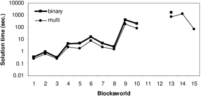
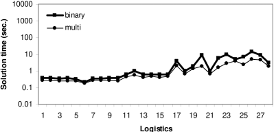
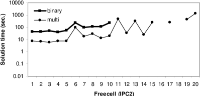
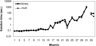
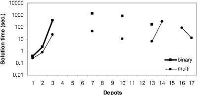
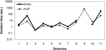
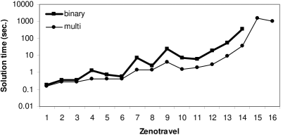
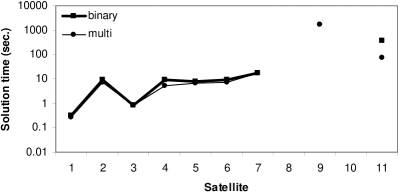
Figure 19: Comparing binary state descriptions with multi-valued state descriptions using the G1SC formulation.

6 Related Work

There are only few integer programming-based planning systems. Bylander (?) considers an IP formulation based on converting the propositional representation given by Satplan (?) to an IP formulation with variables that take the value 1 if a certain proposition is true, and 0 otherwise. The LP relaxation of this formulation is used as a heuristic for partial order planning, but tends to be rather time-consuming. A different IP formulation is given by Vossen et al. (?). They consider an IP formulation in which the original propositional variables are replaced by state change variables. State change variables take the value 1 if a certain proposition is added, deleted, or persisted, and 0 otherwise. Vossen et al. show that the formulation based on state change variables outperforms a formulation based on converting the propositional representation. Van den Briel and Kambhampati (?) extend the work by Vossen et al. by incorporating some of the improvements described by Dimopoulos (?). Other integer programming approaches for planning rely on domain-specific knowledge (?, ?) or explore non-classical planning problems (?, ?).

In our formulations we model the transitions of each state variable as a separate flow problem, with the individual problems being connected through action constraints. The Graphplan planner introduced the idea of viewing planning as a network flow problem, but it did not decompose the domain into several loosely coupled components. The encodings that we described are related to the loosely-coupled modular planning architecture by Srivastava, Kambhampati, and Do (?), as well as factored planning approaches by Amir and Engelhardt (?), and Brafman and Domshlak (?). The work by Brafman and Domshlak, for example, proposes setting up a separate CSP problem for handling each factor. These individual factor plans are then combined through a global CSP. In this way, it has some similarities to our work (with our individual state variable flows corresponding to encodings for the factor plans). Although Brafman and Domshlak do not provide empirical evaluation of their factored planning framework, they do provide some analysis on when factored planning is expected to do best. It would be interesting to adapt their minimal tree-width based analysis to our scenario.

The branch-and-cut concept was introduced by Grötschel, Rünger, and Reinelt (?) and Padberg and Rinaldi (?), and has been successfully applied in the solution of many hard large-scale optimization problems (?). In planning, approaches that use dynamic constraint generation during search include RealPlan (?) and LPSAT (?).

Relaxed definitions for Graphplan-style parallelism have been investigated by several other researchers. Dimopoulos et al. (?) were the first to point out that it is not necessary to require two actions to be independent in order to execute them in the same plan period. In their work they introduce the property of post-serializability of a set of actions. A set of actions $A^{\prime}\subseteq A$ is said to be post-serializable if (1) the union of their preconditions is consistent, (2) the union of their effects is consistent, and (3) the preconditions-effects graph is acyclic. Where the preconditions-effects graph is a directed graph that contains a node for each action in $A^{\prime}$, and an arc $(a,b)$ for $a,b\in A^{\prime}$ if the preconditions of $a$ are inconsistent with the effects of $a$. For certain planning problems Dimopoulos et al. (?) show that their modifications reduce the number of plan periods and improve performance. Rintanen (?) provides a constraint-based implementation of their idea and shows that the improvements hold over a broad range of planning domains.

Cayrol et al. (?) introduce the notion of authorized linearizations, which implies an order for the execution of two actions. In particular, an action $a\in A$ authorizes an action $b\in A$ implies that if $a$ is executed before $b$, then the preconditions of $b$ will not be deleted by $a$ and the effects of $a$ will not be deleted by $b$. The notion of authorized linearizations is very similar to the property of post-serializability. If we were to adopt these ideas in our network-based representations it would compare to the G1SC network in which the generalized state change arcs (see Figure 7) only allows values to prevail after, but not before, each of the transition arcs.

A more recent discussion on the definitions of parallel plans is given by Rintanen, Heljanko and Niemelä (?). Their work introduces the idea of $\exists$-step semantics, which says that it is not necessary that all parallel actions are non-interfering as long as they can be executed in at least one order. $\exists$-step semantics provide a more general interpretation of parallel plans than the notion of authorized linearizations used by LCGP (?). The current implementation of $\exists$-step semantics in Satplanner is, however, somewhat restricted. While the semantics allow actions to have conflicting effects, the current implementation of Satplanner does not.

7 Conclusions

This work makes two contributions: (1) it improves state of the art in modeling planning as integer programming, and (2) it develops novel decomposition methods for solving bounded length (in terms of number of plan periods) planning problems.

We presented a series of IP formulations that represent the planning problem as a set of loosely coupled network flow problems, where each network flow problem corresponds to one of the state variables in the planning domain. We incorporated different notions of action parallelism in order to reduce the number of plan periods needed to find a plan and to improve planning efficiency. The IP formulations described in this paper have led to their successful use in solving partial satisfaction planning problems (?). Moreover, they have initiated a new line of work in which integer and linear programming are used in heuristic state-space search for automated planning (?, ?). It would be interesting to see how our approach in the context of IP formulations applies to formulations based on satisfiability and constraint satisfaction.

Acknowledgments

This research is supported in part by the NSF grant IIS 308139, the ONR grant N000140610058, and by the Lockheed Martin subcontract TT0687680 to Arizona State University as part of the DARPA integrated learning program. We thank Derek Long for his valuable input, and we especially thank the anonymous reviewers whose attentive comments and helpful suggestions have greatly improved this paper.

References

- Amir & Engelhardt Amir, E., & Engelhardt, B. (2003). Factored planning. In Proceedings of the 18th International Joint Conference on Artificial Intelligence (IJCAI-2003), pp. 929–935.
- Bäckström & Nebel Bäckström, C., & Nebel, B. (1995). Complexity results for SAS+ planning. Computational Intelligence, 11(4), 625–655.
- Benton et al. Benton, J., van den Briel, M., & Kambhampati, S. (2007). A hybrid linear programming and relaxed plan heuristic for partial satisfaction planning problems. In Proceedings of the International Conference on Automated Planning and Scheduling (ICAPS-2007), pp. 34–41.
- Bixby Bixby, R. E. (2002). Solving real-world linear programs: a decade and more of progress. Operations Research, 50(1), 3–15.
- Blum & Furst Blum, A., & Furst, M. (1995). Fast planning through planning graph analysis. In Proceedings of the 14th International Joint Conference on Artificial Intelligence (IJCAI-1995), pp. 1636–1642.
- Bockmayr & Dimopoulos Bockmayr, A., & Dimopoulos, Y. (1998). Mixed integer programming models for planning problems. In Working notes of the CP-98 Constraint Problem Reformulation Workshop.
- Bockmayr & Dimopoulos Bockmayr, A., & Dimopoulos, Y. (1999). Integer programs and valid inequalities for planning problems. In Proceedings of the European Conference on Planning (ECP-1999), pp. 239–251.
- Brafman & Domshlak Brafman, R., & Domshlak, C. (2006). Factored planning: How, when, and when not. In Proceedings of the 21st National Conference on Artificial Intelligence (AAAI-2006), pp. 809–814.
- Bylander Bylander, T. (1997). A linear programming heuristic for optimal planning. In Proceedings of the 14th National Conference on Artificial Intelligence (AAAI-1997), pp. 694–699.
- Caprara & Fischetti Caprara, A., & Fischetti, M. (1997). Annotated Bibliographies in Combinatorial Optimization, chap. Branch and Cut Algorithms, pp. 45–63. John Wiley and Sons.
- Cayrol et al. Cayrol, M., Régnier, P., & Vidal, V. (2001). Least commitment in graphplan. Artificial Intelligence, 130(1), 85–118.
- Desaulniers et al. Desaulniers, G., Desrosiers, J., & Solomon, M. (Eds.). (2005). Column Generation. Springer.
- Dimopoulos Dimopoulos, Y. (2001). Improved integer programming models and heuristic search for AI planning. In Proceedings of the European Conference on Planning (ECP-2001), pp. 301–313.
- Dimopoulos & Gerevini Dimopoulos, Y., & Gerevini, A. (2002). Temporal planning through mixed integer programming. In Proceedings of the Workshop on Planning for Temporal Domains (AIPS-2002), pp. 2–8.
- Dimopoulos et al. Dimopoulos, Y., Nebel, B., & Koehler, J. (1997). Encoding planning problems in nonmonotic logic programs. In Proceedings of the 4th European Conference on Planning (ECP-1997), pp. 167–181.
- Do et al. Do, M., Benton, J., van den Briel, M., & Kambhampati, S. (2007). Planning with goal utility dependencies. In Proceedings of the 20th International Joint Conference on Artificial Intelligence (IJCAI-2007), pp. 1872–1878.
- Edelkamp & Helmert Edelkamp, S., & Helmert, M. (1999). Exhibiting knowledge in planning problems to minimize state encoding length. In Proceedings of the European Conference on Planning (ECP-1999), pp. 135–147.
- Garey & Johnson Garey, M., & Johnson, D. (1979). Computers and Intractability: a Guide to the Theory of NP-Completeness. Freeman and Company, N.Y.
- Grötschel et al. Grötschel, M., Jünger, M., & Reinelt, G. (1984). A cutting plane algorithm for the linear ordering problem. Operations Research, 32, 1195–1220.
- Helmert Helmert, M. (2006). The Fast Downward planning system. Journal of Artifical Intelligence Research, 26, 191–246.
- Hooker Hooker, J. (1988). A quantitative approach to logical inference. Decision Support Systems, 4, 45–69.
- ILOG Inc. ILOG Inc., Mountain View, CA (2002). ILOG CPLEX 8.0 user’s manual.
- Johnson et al. Johnson, E., Nemhauser, G., & Savelsbergh, M. (2000). Progress in linear programming based branch-and-bound algorithms: An exposition. INFORMS Journal on Computing, 12, 2–23.
- Kambhampati & commentary from other planning researchers Kambhampati, S., & commentary from other planning researchers (2006). On the suboptimality of optimal planning track at ipc 2006. http://raos-ruminations.blogspot.com/2006/07/on-suboptimality-of-optimal-planning.html.
- Karmarkar Karmarkar, N. (1984). A new polynomial time algorithm for linear programming. Combinatorica, 4(4), 373–395.
- Kautz Kautz, H. (2004). SATPLAN04: Planning as satisfiability. In Working Notes on the Fourth International Planning Competition (IPC-2004), pp. 44–45.
- Kautz & Selman Kautz, H., & Selman, B. (1992). Planning as satisfiability. In Proceedings of the European Conference on Artificial Intelligence (ECAI-1992).
- Kautz & Selman Kautz, H., & Selman, B. (2006). SATPLAN04: Planning as satisfiability. In Working Notes on the Fifth International Planning Competition (IPC-2006), pp. 45–46.
- Kautz & Walser Kautz, H., & Walser, J. (1999). State-space planning by integer optimization. In Proceedings of the 16th National Conference on Artificial Intelligence (AAAI-1999), pp. 526–533.
- Martin Martin, K. (1991). Using separation algorithms to generate mixed integer model reformulations. Operations Research Letters, 10, 119–128.
- Padberg & Rinaldi Padberg, M., & Rinaldi, G. (1991). A branch-and-cut algorithm for the resolution of large-scale symmetric traveling salesman problems. SIAM Review, 33, 60–100.
- Rintanen Rintanen, J. (1998). A planning algorithm not based on directional search. In Proceedings of the Sixth International Conference on Principles of Knowledge Representation and Reasoning (KR-1998), pp. 617–624.
- Rintanen et al. Rintanen, J., Heljanko, K., & Niemelä, I. (2006). Planning as satisfiability: parallel plans and algorithms for plan search. Artificial Intelligence, 170(12), 1031–1080.
- Srivastava et al. Srivastava, B., Kambhampati, S., & Do, M. (2001). Planning the project management way: Efficient planning by effective integration of causal and resource reasoning in realplan. Artificial Intelligence, 131(1-2), 73–134.
- van den Briel et al. van den Briel, M., Benton, J., Kambhampati, S., & Vossen, T. (2007). An LP-based heuristic for optimal planning. In Proceedings of the International Conference of Principles and Practice of Constraint Programming (CP-2007), pp. 651–665.
- van den Briel & Kambhampati van den Briel, M., & Kambhampati, S. (2005). Optiplan: Unifying IP-based and graph-based planning. Journal of Artificial Intelligence Research, 24, 623–635.
- van den Briel et al. van den Briel, M., Kambhampati, S., & Vossen, T. (2007). Fluent merging: A general technique to improve reachability heuristics and factored planning. In Proceedings of the Workshop Heuristics for Domain-Independent Planning: Progress, Ideas, Limitations, Challenges (ICAPS-2007).
- Vossen et al. Vossen, T., Ball, M., Lotem, A., & Nau, D. (1999). On the use of integer programming models in AI planning. In Proceedings of the 18th International Joint Conference on Artificial Intelligence (IJCAI-1999), pp. 304–309.
- Wolfman & Weld Wolfman, S., & Weld, D. (1999). The LPSAT engine and its application to resource planning. In Proceedings of the 18th International Joint Conference on Artificial Intelligence (IJCAI-1999), pp. 310–317.
- Wolsey Wolsey, L. (1998). Integer Programming. John Wiley and Sons.