On group actions with simple Lebesgue spectrum

Abstract.

In work [22] a set of ergodic flows with simple Lebesgue spectrum is found, and the construction of these flows is based on the phenomenon of existence of Littlewood-type flat polynomials with coefficients $0$ and $1$ on the group ${\mathbb{R}}$, which is closely related to the algebraic and arithmetic properties of ${\mathbb{R}}$ as a field. Thus, if we think about a hypothetical extension of this phenomenon to general Abelian groups and its futher applications to ergodic group actions with simple Lebesgue spectrum, the method used in [22] could be applied to a very specific class of groups including, for example, $p$-adic fields. At the same time, in some cases it is posible to generalize the flatness phenomenon applying a sort of straightforward analytic technique. In this paper we illustrate this argument and propose a method of such kind that helps to pass from the case of the group ${\mathbb{R}}$ to its Cartesian product ${\mathbb{R}}^{d}$. We establish the existence of ${\mathbb{R}}^{d}$-actions with Lebesgue spectrum of multiplicity one using the synthesis of the original construction of a flow introduced in [22] and this new analytic method.

The work is supported by grants RFFI No.  11-01-00759-a.

Keywords: spectral theory, rank one, ergodic flows, ergodic group actions, $(C,F)$-actions, mixing, simple Lebesgue spectrum, Littlewood polynomials, Riesz products, diophantine approximations

1. Introduction. Rank one flows with simple Lebesgue spectrum

1.1. Spectral invariants of ergodic group actions

Let us consider an invertible transformation $T$ of the standard Lebesgue probability space $(X,\mu)$ preserving measure $\mu$. We require that ${T\colon\>X\to X}$ is an invertible map such that both $T$ and $T^{-1}$ are measurable and ${\mu(TA)=\mu(T^{-1}A)=\mu(A)}$ for any measurable set $A$. It follows from Rokhlin’s theorem (see [23]) that without loss of generality we can assume that $(X,\mu)$ is the unit segment $[0,1]$ with the standard Lebesgue measure.

The Koopman operator $\hat{T}$ in $L^{2}(X,\mu)$ associated with $T$ (see [16, 17]) is defined as

(1) $$\hat{T}\colon\>\varphi({\boldsymbol{x}})\to\varphi(T{\boldsymbol{x}}),\qquad{\boldsymbol{x}}\in X,\quad\varphi\in L^{2}(X,\mu).$$

Clearly, $\hat{T}$ is a unitary operator, hence, by spectral theorem $\hat{T}$ is identified up to unitary equivalence by the measure of maximal spectral type $\sigma$ and the multiplicity function ${\mathcal{M}}(z)$. The spectral type $\sigma$ of a unitary operator is a Borel measure on the unit circle in the complex plane. A great progress made in the spectral theory of measure preserving transformations and group actions during last years (e.g. see [4, 5, 8, 14, 17]), though the it is still a complicated problem to classify the pairs $(\sigma,{\mathcal{M}}(z))$ that can appear as spectral invariants of some dynamical system.

In this paper we deal mainly with measure preserving actions $T^{t}$ of the group ${\mathbb{R}}$, refered to as measurable flows, as well as ${\mathbb{R}}^{d}$-actions. The spectral invariants $(\sigma,\,{\mathcal{M}}(z))$ of the unitary representation ${\hat{T}}^{t}$ associated with an ${\mathbb{R}}^{d}$-action are defined in the same way like in the case of a single unitatry operator, but in this case the measure of maximal spectral type $\sigma$ is a Borel measure on ${{\widehat{{\mathbb{R}}}}^{d}={\mathbb{R}}^{d}}$.

1.2. Rank one flows

Let us consider an increasing sequence $(h_{n})_{n=1}^{\infty}$, ${h_{n}>0}$, and the corresponding sequence of segments ${I_{n}=[0,h_{n+1}]}$. Suppose that for each $n$ a finite collection of disjoint subintervals

(2) $$(\omega_{n}(j),\omega_{n}(j)+h_{n})\subset I_{n+1},\qquad j=0,\dots,q_{n}-1,$$

is given such that ${\omega_{n}(j)+h_{n}\leq\omega_{n}(j+1)}$, and define the corresponding projection ${\phi_{n}\colon\>I_{n+1}\to I_{n}}$ such that ${\phi_{n}(\omega_{n}(j)+t)=t}$ for any $j$ and ${0\leq t\leq h_{n}}$ and ${\phi_{n}(t_{n+1})=0}$ otherwise. Notice that $\phi_{n}$ is continuous as a map from $I_{n+1}$ to $I_{n}$ if we identify edge points $0$ and $h_{n}$, i.e. .  .if we consider $\phi_{n}$ as a continuious map of degree $q_{n}$ from the circle ${\mathbb{R}}/h_{n+1}{\mathbb{Z}}$ to the circle ${\mathbb{R}}/h_{n}{\mathbb{Z}}$. The map $\phi_{n}$ is a linear map with derivative $1$ at any interval ${(\omega_{n}(j),\omega_{n}(j)+h_{n})}$, and $\phi_{n}$ is constant on the complement to these intervals. In other words, $\phi_{n}$ is a formal representation of the following dynamical process: a point $x_{n}(t)$ moves in the segment $I_{n}$ with the velocity $1$ and after arriving to the right edge $h_{n}$ of the segment the point $x_{n}(t)$ waits for time

(3) $$s_{n,j}=\omega_{n}(j+1)-\omega_{n}(j)-h_{n}$$

depending on the index $j$, and after this time is passed continues moving from the left edge $0$ of the segment $I_{n}$. The values $s_{n,j}$ in terms of cutting-and-stacking construction are called spacers between subsequent subintervals $(\omega_{n}(j),\omega_{n}(j)+h_{n})$ (recall that the edge points are topologically identified).

Figure 1. Construction of a rank one flow: definition of the projection $\phi_{n}$

Let us define the phase space $X$ of the flow to be the inverse limit of the spaces $(I_{n},{\mathcal{B}}_{n})$ endowed with the Borel $\sigma$-algebra ${\mathcal{B}}_{n}$ with respect to the maps $\phi_{n}$, i.e. .  .set

(4) $$X=\{{\boldsymbol{x}}=(x_{1},x_{2},\dots,x_{n},\dots)\colon\>x_{n}\in I_{n},.\,.\phi_{n}(x_{n+1})=x_{n}\}.$$

The following condition ensures the correctness of the construction:

(5) $$\prod_{n=1}^{\infty}\frac{h_{n+1}}{q_{n}h_{n}}<\infty.$$

Namely, if (5) is satisfied then there exist measures ${\mu_{n}=(1-\gamma_{n})\lambda_{n}+\gamma_{n}\delta_{0}}$, ${\gamma_{n}\to 0}$ as ${n\to\infty}$ and ${d\lambda_{n}=h_{n}^{-1}dt}$, such that ${\phi_{n}^{*}\mu_{n+1}=\mu_{n}}$, and we can define the measure $\mu$ on the limit space $X$ coinciding with $\mu_{n}$ after projecting to $I_{n}$ (see [21] for further technical details).

Now let us define the map $T$ on the space $(X,\mu)$ as follows. Let us fix ${t\in{\mathbb{R}}}$. For almost every point ${{\boldsymbol{x}}=(x_{1},x_{2},\dots,x_{n},\dots)}$ in $X$ the following is true: ${|t|<x_{n}<h_{n}-|t|}$ starting from some index $n_{0}$. We define $Tx$ by the relation

(6) $$(Tx)_{n=n_{0}}^{\infty}=(x_{n_{0}}+t,\dots,x_{n}+t,\dots)$$

and complete the sequence of coordinates $(Tx)_{n}$ for indexes $n$ smaller than $n_{0}$ using the fundamental relation ${\phi_{n}((Tx)_{n+1})=(Tx)_{n}}$. It can be easily verified that $T$ is an invertible measurable transformation on $X$ preserving the measure $\mu$.

1.3. Flows with simple Lebesgue spectrum and Littlewood polynomials

Theorem 1 (see [22]).

There exist rank one flows with simple Lebesgue spectrum.

The principal analytic argument that we can use to find a rank one flow with Lebesgue spectrum is the flatness phenomenon for the class of polynomials on the group ${\mathbb{R}}$

(7) $${\mathcal{M}}^{{\mathbb{R}}}=\Bigl{\{}{\mathcal{P}}(\tau)=\frac{1}{\sqrt{q}}\sum_{y=0}^{q-1}e^{2\pi i\,\tau\omega(y)}\colon\>\omega(y)<\omega(y+1),.\,.\omega(y)\in{\mathbb{R}},.\,.q\geq 2\Bigr{\}}$$

called Littlewood polynomials with coefficients in $\{0,1\}$. This question goes back to the famous work due to J. Littlewood [18] (see also [10]) as well as investigations on Hardy–Littlewood series [28]. The Littlewood’s hyposesis on flat polynomials is asking whether one can find a unimodular polynomial

(8) $$P(z)=\frac{1}{\sqrt{N}}\sum_{n=0}^{N-1}a_{n}z^{n},\qquad|a_{n}|=1,\qquad N\geq 2,$$

such that $P(z)$ is $\varepsilon$-ultraflat on the unit circle in the complex plane for any given $\varepsilon\>$?

A complex polynomial $P(z)$ is called $\varepsilon$-ultraflat if

(9) $$\max_{z\in S^{1}}\>\Bigl{|}\,|P(z)|-1\,\Bigr{|}<\varepsilon,\qquad S^{1}=\{z\in{\mathbb{C}}\colon\>|z|=1\}.$$

This question was answered positively by J.-P. Kahane [13], though, the problem of flatness in the class of polynomials with coefficients in $\{-1,+1\}$ as well as in the class ${\mathcal{M}}^{{\mathbb{Z}}}$ of polynomials with coeffitients in $\{0,1\}$ is wide open (for references and discussion see [3], [9], [10], [11], [22]). It is shown in paper [22] that in contrast to the classical flatness problem if ${\mathcal{M}}^{{\mathbb{Z}}}$ that looks rather difficult and no reasonable arguments are known for the answer to be “yes” or “no”, if we pass to the class ${\mathcal{M}}^{{\mathbb{R}}}$ of polynomials on ${\mathbb{R}}$ the answer in “yes” in $L^{1}$-sense on any compact subset of ${\mathbb{R}}$ and one can find explicit examples of flat sums.

Definition 2.

Let us call a window a set of two symmetric intervals isolated both from $0$ and infinity:

(10) $$G=(-b,-a)\cup(a,b),\qquad 0<a<b.$$

Definition 3.

We say that a polynomial ${\mathcal{P}}(t)$ on the real line ${\mathbb{R}}$ is $\varepsilon$-flat in $L^{p}(G)$ (or $L^{p}(G)$-$\varepsilon$-flat) if

(11) $$\bigl{\|}\>|{\mathcal{P}}(\tau)|-1\>\bigr{\|}_{L^{p}(G)}<\varepsilon.$$

Theorem 4 (see [22]).

For any ${\varepsilon>0}$ and a window $G$ there exists a polynomial ${\mathcal{P}}(t)$ which is $\varepsilon$-flat both in $L^{1}(G)$ and $L^{2}(G)$ and satisfies estimate ${|{\mathcal{P}}(t)|\leq M}$ for ${t\in G}$ with a global constant $M$.

It is interesting to see that the flat polynomials in theorem 4 can be represented in an explicit way.

Theorem 5 (see [22]).

Let us fix a window $G$ and some precision ${\varepsilon>0}$. There exists ${m>0}$ and ${\beta_{0}>0}$ such that for any ${\beta\leq\beta_{0}}$, ${\beta^{-1}\in{\mathbb{N}}}$, there exists an infinite sequence ${\bar{q}=(q_{j})_{j=1}^{\infty}}$ of polynomial degrees generating $L^{1}$-$\varepsilon$-flat polynomials on $G$

(12) $${\mathcal{P}}_{q}(\tau)=\frac{1}{\sqrt{q}}\sum_{y=0}^{q-1}e^{2\pi i\,t\omega(y)}\quad\text{with}\quad\omega(y)=m\frac{q}{\beta^{2}}e^{\beta y/q}.\qquad q\in\bar{q}.$$

Remark 6.

The only feature which is hard to control when choosing parameters $m$, $\beta$ and $q$ in theorem 5 is the sequence $q_{j}$. Indeed, the sequence $q_{j}$ is the rarer the smaller $\varepsilon$ and the more spacious window $G$ we take. Here we use the term spaciousness of the window $G$ for the fraction $b/a$. Suprisingly the value of the  smallest .  .proper $q$ is strongly related to the diophantine properties of the vector

(13) $${\boldsymbol{v}}=(\log 2,\log 3,\log 4,\dots,\log(K+1)).$$

More exactly, we consider the line parallel to ${\boldsymbol{v}}$ in the torus ${\mathbb{T}}^{K}$ starting from $0$ and study its first return time to some $\varepsilon$-neighbourhood of the zero point. And the value of this return time is connected with the complexity (in particulr, the degree) of the polynomial ${\mathcal{P}}(\tau)$. To explain this phenomenon we should mention that the frequency function $\omega(y)$ in the proof of theorem 5 is considered a Hamiltonian of a free quantum particle moving on the torus ${\mathbb{T}}$, and the small parameter $\beta q^{-1}$ measures deviation according to the classical quadratic Hamiltonian ($y$ is the momentum of the particle),

(14) $$\omega(y)={\color[rgb]{0,1,0}\frac{q}{\beta^{2}}+\frac{y}{\beta}}+{\color[rgb]{0,0,1}\frac{y^{2}}{2q}}+{\color[rgb]{0,0,0}\beta\frac{y^{3}}{6q^{2}}+\dots,}$$

where $m=1$, for example. Actually, that is exactly $\beta^{-1}q$, the value playing role of a time in the dynamical system ${\dot{Y}={\boldsymbol{v}}(Y)}$ on the torus ${\mathbb{T}}^{K}$ participating in the construction of flat polynomials with the frequency function ${\omega=\frac{q}{\beta^{2}}e^{\beta y/q}}$.

The following theorem generalizing lemma 5 is of special status concerning the content of this paper. It cannnot used to improve the investigation of Riesz products on ${\mathbb{R}}$, but it is applied in the case of rank one ${\mathbb{R}}^{d}$-actions (see the proof of theorem 33 and lemma 34).

Theorem 7.

For any compact set $K$ in ${\mathbb{R}}$ and ${\varepsilon>0}$ there exists a polinomial in the class ${\mathcal{M}}^{{\mathbb{R}}}$ which is $\varepsilon$-flat in $L^{1}(K)$.

Observe that the statement of this lemma is false in $L^{2}$, and concerning $L^{1}$-flatness it is not known can we find a polynomial which is globally $L^{1}$-flat on ${\mathbb{R}}\>$?

1.4. Generalized Riesz products and spectral measures of rank one flows

In view of the forthcoming discussion of rank one ${\mathbb{R}}^{d}$-actions we consider in detains the proof of theorem 1 in the one-dimensional case. The concept of generalized Riesz product in the scope of rank one dynamical systems goes back to paper [6] by J. Bourgain. In this paper the measure of maximal spectral type $\sigma$ is claculated for the mixing rank one constructions introduced by D. Ornstein [19]. The measure $\sigma$ is represented in a form of Riesz product (converging in weak sense)

(15) $$\sigma=\prod_{n=1}^{\infty}|P_{n}(z)|^{2},\qquad P_{n}(z)=\frac{1}{\sqrt{q_{n}}}\sum_{k=0}^{q_{n}-1}z^{\omega_{n}(k)}$$

and it is discovered that this measure in purely singular with probability $1$ (see also [1, 2, 3]).

It is important to mention the deep connection of this approach with the classical problem on investigation of purely singular Rajchman measures on the unit segment $[0,1]$, in particular, the famous question due to Rafaël Salem on the Minkowskii question mark function and his work on strictly increasing singular functions on $[0,1]$ with fast correlation decay (see [25, 26] and [12]). In order to illustrate this connection let us mention that in the most cases the spectral measures of rank one dynamical systems are investigated using different variations around the Riesz product technique, though, it is not known exactly how fast the Fourier coefficients

(16) $$c_{n}=\int_{0}^{1}e^{2\pi i\,nx}\,d\sigma(x)$$

can decay for the spectral measures $\sigma$ of rank one dynamical systems? At the same time, for a class of local rank one ergodic transformations (see [20]) one can observe the extremal rate of power decay

(17) $$c_{n}=O(n^{-1/2+\varepsilon})$$

for all ${\varepsilon>0}$, similar to R. Salem’s examples of purely singular measures on $[0,1]$. Notice that faster power decay (with some additional requirements) would ensure the absolute continuity of the spectral measure $\sigma$. Nevertheless, no deducion can be made from such kind of information about the decay of $c_{n}$, whether it has a Lebesgue component or not?

Hypothesis 8.

Suppose that a sequence of tower partitions $\xi_{n}$ is fixed for a rank one transformation such that $\xi_{n+1}$ refines $\xi_{n}$ and any measurable set $A$ can be approximated by a sequence of $\xi_{n}$-measurable sets $A_{n}$. Then for any $\xi_{n_{0}}$-measurable function $f$ the sequence of the Fourier coefficients $c_{n}$ for the spectral measure $\sigma_{f}$ satisfies

(18) $$\limsup_{n\to\infty}\frac{\log|c_{n}|}{n}\geq-\frac{1}{2}.$$

Enclosing the discussion around analytical properties of the spectral measures generated by rank one dynamical systems let us remark that if we like construct a Lebesgue component in the spectrum of some rank one system, the only approach discussed in the literature (both for transformatios and flows) is the use of Littlewood-type flat polynomials. THough, hypothetically it could happen that $P_{n}(z)$ are not flat, but the Riesz product (15) converges to a measure with an absolutely continuous component or even Lebesgue measure. In this connection we should mention that the following question concerning the spectral type of rank one transformations is still open.

Question 9.

For any rank one transformation the measure of maximal spectral type $\sigma$ is singular with respect to the Lebesgue measure?

Question 10 (S. Banach).

Is it possible to find an invertible measure preserving transformation with the Lebesgue spectrum of multiplicity one?

Therefore a rank one transformation is a candidate to the positive answer to the well-known question 10 due to Stephan Banach (see [27], [15], [17] and [22]), there are no obstacles both for question 9 and for question on existence of Littlewood type flat polynomials in the class ${\mathcal{M}}$ to be false. At the same time, both questions, the flatness in the class ${\mathcal{M}}^{{\mathbb{R}}}$ and Banach question, have positive answer for the group ${\mathbb{R}}$, and our purpose in this paper is to discuss simple extensions of this phenomenon to the larger class of group actions including a class of rank one ${\mathbb{R}}^{d}$-actions.

Proof of theorem 1. Let us consider a function ${f\colon\>X\to{\mathbb{C}}}$, ${f\in L^{2}(X,\mu)}$, which is measurable with respect to $\sigma$-algebra ${\mathcal{B}}_{n}$. Such function can be represented in the form

(19) $$f({\boldsymbol{x}})=f_{(n_{0})}(x_{n_{0}}),$$

where $x_{n_{0}}$ is the $n_{0}$-th coordinate of a point ${{\boldsymbol{x}}\in X}$. The function $f_{n_{0}}$ as well as any measurable function on $I_{n}$ can be lifted to the upper levels in accordance with the relation

(20) $$f_{(n+1)}(x_{n+1})=f_{(n)}(\phi_{n}(x_{n+1})).$$

Here and in the sequel we consider the functions $f_{(n)}(x_{n})$ like function on the real line ${\mathbb{R}}$ letting $f_{(n)}$ be zero outside ${I_{n}=[0,h_{n}]}$. Let us define the following correlation functions:

(21) $$R(t)=\left\langle T^{t}f,\,f\right\rangle,$$

(22) $$R_{n}(t)=(1-\gamma_{n})\frac{1}{h_{n}}\int_{0}^{h_{n}}f_{(n)}(t+x_{n})\,\overline{f_{(n)}(x_{n})}\,dx_{n},\quad n\geq n_{0},$$

and recall that the equivariant measure $\mu_{n}$ on the $n$-th level of the construction of the rank one flow equals ${(1-\gamma_{n})\lambda_{n}+\gamma_{n}{\boldsymbol{\delta}}_{0}}$ and ${1-\gamma_{n}}$ is the total measure of the $n$-th tower in the cutting-and-stacking construction,

(23) $$1-\gamma-n=\mu(U_{n}),\quad\text{where}\quad U_{n}=\{{\boldsymbol{x}}\in X\colon\>0<x_{n}<h_{n}\}.$$

Without loss of generality for our purposes it suffies to explore functions satisfying the following requirements:

• ${|f({\boldsymbol{x}})|\leq M_{0}}$;

• ${\|f\|=1}$ in $L^{2}(X,\mu)$;

• ${f({\boldsymbol{x}})=0}$ outside the tower $U_{n}$.

From this point we assume that these conditions are satisfied. Notice that ${R(0)=\|f\|^{2}=1}$ and we can also check that ${R_{n}(0)=1}$.

Lemma 11.

$R_{n}(0)=1$ for any $n\geq n_{0}$.

Proof.

The lemma follows from the observation that $f_{(n+1)}$ “sits inside” any tower $U_{n}$ with ${n\geq n_{0}}$, whenever ${\mathop{\mathrm{supp}}\nolimits f_{(n_{0})}\subseteq U_{n_{0}}}$ (up to zero measure set) for some starting index $n_{0}$. Thus, for any ${\mathcal{B}}_{n}$-measurable function ${\psi({\boldsymbol{x}})\in L^{1}(X,\mu)}$, zero on ${X\mathbin{\smallsetminus}U_{n}}$, which is associated with a function $\psi_{(n)}$ on $[0,h_{n}]$ we have

(24) $$\int_{X}\psi({\boldsymbol{x}})\,d\mu=\frac{1-\gamma_{n}}{h_{n}}\int_{0}^{h_{n}}\psi(x)\,dx.$$

and the statement follows from the identity ${R_{n}(0)=\|\psi_{(n)}\|^{2}}$, since $R_{n}(t)$ is the correlation function for the shift action

(25) $$S^{t}\colon\>{\mathbb{R}}\to{\mathbb{R}}\colon\>x\mapsto t+x,$$

where $\|\psi_{(n)}\|$ is the norm in $L^{2}({\mathbb{R}},\,(1-\gamma_{n})h_{n}^{-1}dx)$. ∎

Since the sequence towers $U_{n}$ approximate the $\sigma$-algebra of our phase space $(X,\mu)$ and $U_{n}$ covers most part of $X$, i.e. .  .${\mu(U_{n})\to 1}$, the functions $R_{n}(t)$ asymptotically close to $R(t)$.

Lemma 12.

If $0<|t|<h_{n}$ then ${|R_{n}(t)-R(t)|\leq\gamma_{n}+|t|/h_{n}}$.

Proof.

Indeed, integrating the product $f_{(n)}(t+x_{n})\,\overline{f_{(n)}(x_{n})}$ in $R(t)$ we cannot control the influence of the set of measure $\gamma_{n}$ outside $U_{n}$ and the part of the tower $U_{n}$ not covered by the levels that fit into the overlapping ${I_{n}\cap(I_{n}+t)}$. Suppose that ${t>0}$, then

(26) $$R(t)=\int_{U_{n}}T^{t}f({\boldsymbol{x}})\,\overline{f({\boldsymbol{x}})}\,d\mu({\boldsymbol{x}})+\int_{X\mathbin{\smallsetminus}U_{n}}T^{t}f({\boldsymbol{x}})\,\overline{f({\boldsymbol{x}})}\,d\mu({\boldsymbol{x}})=\\ =\frac{1-\gamma_{n}}{h_{n}}\int_{0}^{h_{n}-t}f_{(n)}(t+x_{n})\,\overline{f_{(n)}(x_{n})}\,dx_{n}+\int_{U_{n}|_{(h_{n}-t,h_{n})}\>\cup\>(X\mathbin{\smallsetminus}U_{n})}T^{t}f({\boldsymbol{x}})\,\overline{f({\boldsymbol{x}})}\,d\mu({\boldsymbol{x}}),$$

where

(27) $$U_{n}|_{J}\stackrel{{\scriptstyle def}}{{=}}\{{\boldsymbol{x}}\in X\colon\>x_{n}\in J\},$$

and

(28) $$R_{n}(t)=\frac{1-\gamma_{n}}{h_{n}}\int_{0}^{h_{n}-t}f_{(n)}(t+x_{n})\,\overline{f_{(n)}(x_{n})}\,dx_{n},$$

hence, taking into account the requirement ${|f|\leq 1}$,

(29) $$|R_{n}(t)-R(t)|\leq\mu\bigl{(}U_{n}|_{(h_{n}-t,h_{n})}\>\cup\>(X\mathbin{\smallsetminus}U_{n})\bigr{)}\leq t/h_{n}+\gamma_{n}.$$

The case ${t<0}$ is symmetrical. ∎

As a direct corollary we get the following statement.

Lemma 13.

For a fixed ${\mathcal{B}}_{n_{0}}$-measurable function $f({\boldsymbol{x}})$ satisfying the conditions stated above then the correlation functions $R_{n}(t)$ converges pointwise to $R(t)$, i.e. .  .

(30) $$\forall t\in{\mathbb{R}}\quad R_{n}(t)\to R(t).$$

The next lemma is the common property of measurable ${\mathbb{R}}$-actions on a Lebesgue space (see [16]).

Lemma 14.

Any measurable flow $T^{t}$ is continuous, i.e. .  .${R_{f}(t)\to 0}$ as ${t\to 0}$ for any ${f\in L^{2}(X,\mu)}$, where ${R_{f}(t)=\left\langle T^{t}f,\,f\right\rangle}$.

Now using the well-known Levy’s lemma we can deduce the convergence of the corresponding probability distributions $\sigma_{n}$, where ${{\widehat{\sigma}}_{n}=R_{n}(t)}$.

Lemma 15 (Levy).

Given a sequence of probability distributions $\nu_{n}$ on ${\mathbb{R}}$ as well as a distribution $\nu^{*}$, if the characteristic functions $\widehat{\nu}_{n}(t)$ converge pointwise to the characteristic function $\widehat{\nu}^{*}$ and the limit funtion $\widehat{\nu}^{*}$ is continuous at zero than $\nu_{n}$ converges weakly to $\nu^{*}$ with respect to the space $C_{b}({\mathbb{R}})$ of bounded continuous functions (with the $C$-norm), i.e. .  .

(31) $$\forall\,\phi(x)\in C_{b}({\mathbb{R}})\quad\int\phi(x)\,d\nu_{n}\to\int\phi(x)\,d\nu.$$

Let us make the following remark. It is important in Levy’s lemma that we know in advance that the limit function ${r(t)=\lim_{n\to\infty}\widehat{\nu}_{n}(t)}$ coincides with the characteristic function of some probability distribution $\nu^{*}$.

Lemma 16.

Any function ${\widehat{R}}_{n}(\tau)$ is a density of a positive measure $\sigma_{n}$ on ${\mathbb{R}}$ and ${\|\sigma_{n}\|=1}$.

Proof.

The first statement follows from the following explicit form of the correlation function for the shift action $S^{t}$:

(32) $$R_{n}(t)=f_{(n)}\stackrel{{\scriptstyle n}}{{\mathbin{*}}}\tilde{f}_{(n)},$$

where ${\tilde{f}_{(n)}(x)=\overline{f_{(n)}(-x)}}$ and the convolution is defined using the same normalizing multiplier like the $L^{2}$-norm on $I_{n}$:

(33) $$(f\stackrel{{\scriptstyle n}}{{\mathbin{*}}}g)(t)=\frac{1-\gamma_{n}}{h_{n}}\int_{{\mathbb{R}}}f(t-x)\,g(x)\,dx.$$

Hence,

(34) $${\widehat{R}}_{n}(\tau)=(f_{(n)}\stackrel{{\scriptstyle n}}{{\mathbin{*}}}\tilde{f}_{(n)})\,\widehat{\hbox{\,}}=\frac{1-\gamma_{n}}{h_{n}}\,|\widehat{f}_{(n)}|^{2}(\tau),$$

and, finally, for the measure $\sigma_{n}={\widehat{R}}_{n}(\tau)\,d\tau$ we have ${\|\sigma_{n}\|=R(0)=1}$. ∎

Let us note that the symbol $\widehat{f}$ means the ordinary Fourier transform,

(35) $$\widehat{f}(\tau)=\int_{{\mathbb{R}}}e^{2\pi i\,\tau\,t}f(t)\,dt,$$

and with the following notation for the normalized Fourier transform

(36) $${\mathsf{F}}_{n}[f](\tau)=\sqrt{\frac{1-\gamma_{n}}{h_{n}^{-1}}}\cdot{\widehat{f}}(\tau).$$

we get the following smart representation for ${\hat{R}}_{n}(t)$:

(37) $${\widehat{R}}_{n}(\tau)=\bigl{|}{\mathsf{F}}[f]_{(n)}\bigr{|}^{2}(\tau).$$

Lemma 17.

The sequence $\sigma_{n}$ converges weakly to the spectral measure $\sigma$.

Proof.

From the spectral theorem we know that $R(t)$ is the (inverse) Fourier transform of the spectral measure $\sigma$, hence, we can apply Levy’s lemma to the sequence $\sigma_{n}$ taking into account continuity at zero of $R(t)$. ∎

Remark 18.

This lemma opens a set of non-trivial effects. For the sake of the forthcoming analytical investigation of the measure $\sigma$ it is important to know that $\sigma_{n}$ a priori converges to $\sigma$. Though, it is hard to follow the sequence of densities ${\widehat{R}}_{n}(\tau)$, for example, if we try to examine the local structure of ${\widehat{R}}_{n}(\tau)$ on an interval $(\tau_{1},\tau_{2})$. The behavior of the densities ${\widehat{R}}_{n}(\tau)$ could be very complicated.

In the case of a rank one transformation it is shown that $\sigma$ can be calculated, in a sense, directly, in the form of generalized Riesz product $\prod_{n}|P_{n}(z)|^{2}$ (see [1, 3, 6]). In other words, there is no need to follow the sequence ${\widehat{R}}_{n}(z)$ for an individual function $f({\boldsymbol{x}})$. On the contrary, the ${\mathbb{R}}$-case is more intriguing, and we need to apply additional restrictions to the huge variety of ${\mathbb{R}}$-based Riesz product. In our case the initial density ${\widehat{R}}_{(n_{0})}(\tau)$ plays the role of regularizing multiplier in the Riesz product. Though, a priory there is no obvious way to eliminate this multiplier and to extract some purely analytic description of the global convergence for the product $\prod_{n}|{\mathcal{P}}_{n}(t)|^{2}$ on the real line ${\mathbb{R}}$. This effect with regard to our case leads to the following phenomenon. In fact, we know a priory that ${\sigma_{n}\to\sigma}$ weakly on ${\mathbb{R}}$, but we can only control the structure of the limit distribution on any window $G_{a,b}={(-b,-a)\cup(a,b)}$, ${a>0}$, and a part of the mass in $\sigma_{n}$ can “escape” into the boundary set

(38) $${\mathcal{F}}={\mathbb{R}}\mathbin{\smallsetminus}\bigcup_{b>a>0}^{\infty}G_{a,b}=\bigl{\{}0\bigr{\}}$$

which is exactly the set containing zero point $\{0\}$. In other words, the limit measure $\sigma$ can have an atom at zero (this is the only possible measure on a one-point set), and to see that $\sigma$ is absolutely continuous we need to apply second ergodic argument, namely, the ergodicity of our rank one flow $T^{t}$ that ensures that $\sigma$ has no atom at zero. Thus, the convergence of $\sigma_{n}$ is established using several argumets coming from the ergodic theory background, and the general question on the global convergence of Riesz products on ${\mathbb{R}}$ is an object for special investigations.

Now we pass to the second logical part of the proof that can be entitled: investigation of the limit distribution $\lim_{n\to\infty}\sigma_{n}$.

Lemma 19.

The densities ${\widehat{R}}_{n}(\tau)$ can be calculated using the following reccurent relation

(39) $${\widehat{R}}_{n+1}(\tau)={\widehat{R}}_{n}(\tau)\cdot|{\mathcal{P}}_{n}(\tau)|^{2},$$

where

(40) $${\mathcal{P}}_{n}(\tau)=\frac{1}{\sqrt{q_{n}}}\sum_{y=0}^{q_{n}-1}e^{2\pi i\,\tau\,\omega_{n}(y)}.$$

Thus,

(41) $${\widehat{R}}_{N+1}(\tau)={\widehat{R}}_{n_{0}}(\tau)\>\prod_{n=n_{0}}^{N}|{\mathcal{P}}_{n}(\tau)|^{2}.$$

Proof.

Since

(42) $$R_{n}(t)=(f_{(n)}\stackrel{{\scriptstyle n}}{{\mathbin{*}}}\tilde{f}_{(n)})(t),$$

it is sufficient to look at the corresponding recurrent formula for $f_{(n)}$. Indeed, it can be easily seen that

(43) $$f_{(n+1)}=f_{(n)}\mathbin{*}({\boldsymbol{\delta}}_{\omega_{n}(0)}+\dots+{\boldsymbol{\delta}}_{\omega_{n}(q_{n}-1)}),$$

hence, passing to Fourier transforms, we have

(44) $${\widehat{f}}_{(n+1)}(\tau)={\widehat{f}}_{(n)}(\tau)\cdot\sum_{y=0}^{q_{n}-1}e^{2\pi i\,\tau\,\omega_{n}(y)}={\widehat{f}}_{(n)}(\tau)\cdot\sqrt{q_{n}}\>P_{n}(\tau),$$

and

(45) $${\widehat{R}}_{n+1}(\tau)=\frac{1-\gamma_{n+1}}{h_{n+1}}\>|{\widehat{f}}_{(n+1)}(\tau)|^{2}=\frac{1-\gamma_{n+1}}{h_{n+1}}\>|{\widehat{f}}_{(n)}(\tau)|^{2}\cdot q_{n}\>|P_{n}(\tau)|^{2}={\widehat{R}}_{n}\cdot|P_{n}(\tau)|^{2}.$$

Here we use the following fundamental relation

(46) $$\frac{h_{n+1}}{q_{n}h_{n}}=\frac{1-\gamma_{n+1}}{1-\gamma_{n}},$$

implying

(47) $$\frac{1-\gamma_{n+1}}{h_{n+1}}\cdot q_{n}=(1-\gamma_{n+1})\cdot\frac{1-\gamma_{n}}{h_{n}\,(1-\gamma_{n+1})}=\frac{1-\gamma_{n}}{h_{n}}$$

and ${\widehat{R}}_{n+1}(\tau)=(1-\gamma_{n})\,h_{n}^{-1}\>|{\widehat{f}}_{(n)}(\tau)|^{2}\cdot|P_{n}(\tau)|^{2}={\widehat{R}}_{n}(\tau)\cdot|P_{n}(\tau)|^{2}$. ∎

Our next purpose is to analyze the convergence of the densities ${\widehat{R}}_{n}(\tau)$ on a window $G_{a,b}$, ${a>0}$, separated from zero. We are going to prove the following common lemma and to apply this observation to the Riesz product for a sequence of flat polynomials ${\mathcal{P}}_{n}(\tau)$.

Lemma 20.

Consider a sequence of positive probability distributions $\nu_{n}$ on ${\mathbb{R}}$ having regular densities ${\rho_{n}\in L^{1}({\mathbb{R}})}$. Suppose that $\nu_{n}$ converges weakly to a probability distribution $\nu^{**}$ and, at the same time, for any segment $[a,b]$, ${a>0}$, the functions $\rho_{n}|_{[a,b]}$ converges in $L^{1}[a,b]$. Then the limit distribution splits into a sum of an absolutely continuous measure and an atom at zero,

(48) $$\nu^{**}=\alpha\,{\boldsymbol{\delta}}_{0}+\Phi(\tau)d\tau,\quad\text{where}\quad\alpha=\nu(\{0\}),$$

moreover, for any segment $[a,b]$, ${a>0}$, the following holds in $L^{1}[a,b]\>$:

(49) $$\lim_{n\to\infty}\rho_{n}|_{[a,b]}=\Phi|_{[a,b]},$$

and $\|\Phi\|_{1}=\nu^{**}({\mathbb{R}}\mathbin{\smallsetminus}\{0\})=1-\alpha$.

The idea of this lemma is very simple. We control the convergence of $\sigma_{n}$ on any window $G_{a,b}$, in fact, $\sigma_{n}$ converge even in strong sense, but some mass can “escape” outside all windows $G_{a,b}$, ${0<a<b}$. Thus, generally we must take into account the atom at zero.

Proof.

First, notice that in our consideration we can omit a set of points which are very far from zero, i.e. .  .using a simple fact of real anaysis we can find ${L>0}$ such that

(50) $$\nu^{**}({\mathbb{R}}\mathbin{\smallsetminus}[-L,L])<\varepsilon$$

for some fixed ${\varepsilon>0}$, since $\nu^{**}$ is a $\Sigma$-finite Borel measure on ${\mathbb{R}}$. Then, roughly speaking, we can restrict ourselves to the compact set $[-L,L]$ and identify measures with the corresponding bounded linear functionals on $C[-L,L]$. We also choose ${\delta>0}$ such that

(51) $$\nu^{**}\bigl{(}(-\delta,0)\cup(0,\delta)\bigr{)}<\varepsilon.$$

Now let us consider a function ${\varphi\in C_{b}({\mathbb{R}})}$ and split $\varphi$ into the sum

(52) $$\varphi=\varphi_{0}+\varphi_{1}+\varphi_{2},\qquad\varphi_{j}(\tau)=r_{j}(\tau)\varphi(\tau),\qquad r_{j}\in C_{b}({\mathbb{R}}),$$

where

(53) $$r_{0}(\tau)+r_{1}(\tau)+r_{2}(\tau)\equiv 1,\qquad|r_{j}(\tau)|\leq 1,$$

(54) $$\mathop{\mathrm{supp}}\nolimits\,r_{0}=[-\delta,\delta],\qquad\mathop{\mathrm{supp}}\nolimits\,r_{1}=G_{\delta/2,L+1},\qquad\mathop{\mathrm{supp}}\nolimits\,r_{2}=(-\infty,-L]\cup[L,\infty),$$

(55) $$r_{1}(\tau)\equiv 1\quad\text{if}\quad\tau\in G_{\delta,L}.$$

For simlicity, let us use notation

(56) $$\left\langle\varphi,\,\nu\right\rangle\stackrel{{\scriptstyle def}}{{=}}\int\varphi(\tau)\,d\nu.$$

We know that

(57) $$\lim_{n\to\infty}\int\varphi(\tau)\,d\nu_{n}=\left\langle\varphi,\,\nu^{**}\right\rangle=\left\langle\varphi_{0},\,\nu^{**}\right\rangle+\left\langle\varphi_{1},\,\nu^{**}\right\rangle+\left\langle\varphi_{2},\,\nu^{**}\right\rangle,$$

and

(58) $$\left|\left\langle\varphi_{0},\,\nu^{**}\right\rangle-\alpha\varphi(0)\right|\leq\varepsilon\cdot\|\varphi\|_{\infty},\qquad\left|\left\langle\varphi_{2},\,\nu^{**}\right\rangle\right|\leq\varepsilon\cdot\|\varphi\|_{\infty},$$

hence,

(59) $$\Bigl{|}\left\langle\varphi,\,\nu^{**}\right\rangle-\left\langle\varphi_{1},\,\nu^{**}\right\rangle-\alpha\varphi(0)\Bigr{|}<2\varepsilon\cdot\|\varphi\|_{\infty}.$$

At the same time, for any component $\varphi_{j}$ we have ${\left\langle\varphi_{j},\,\nu_{n}\right\rangle\to\left\langle\varphi_{j},\,\nu^{**}\right\rangle}$ as ${n\to\infty}$, hence, passing to the limit we see that

(60) $$\left\langle\varphi_{1},\,\nu^{**}\right\rangle=\lim_{n\to\infty}\int_{\delta/2}^{L+1}\varphi(\tau)\,\rho_{n}(\tau)\,d\tau=\int_{\delta/2}^{L+1}\varphi(\tau)\,\Phi|_{[\delta/2,L+1]}(\tau)\,d\tau,$$

where $\Phi|_{[\delta/2,L+1]}$ is the limit of $\rho_{n}$ in $L^{1}[\delta/2,L+1]$. It can be easlily checked that $L^{1}$-limit of $\rho_{n}$ does not depend on the choice of a window $G_{a,b}$, ${a>0}$, so that $\Phi|_{[a,b]}$ is the restriction to $[a,b]$ of some locally $L^{1}$-function $\Phi$ on ${\mathbb{R}}$. More exactly, if ${\rho_{n}\to\Phi_{1}}$ in $L^{1}[a,b]$ and ${\rho_{n}\to\Phi_{2}}$ in $L^{1}[a^{\prime},b^{\prime}]$ for a wider segment ${[a^{\prime},b^{\prime}]\supseteq[a,b]}$ then ${\Phi_{1}=\Phi_{2}|_{[a,b]}}$. Notice that since $\nu_{n}$ converges weakly to $\nu^{**}$

(61) $$\left|\int\varphi_{1}(\tau)\,\Phi(\tau)\,d\tau\right|=\lim_{n\to\infty}|\left\langle\varphi_{1},\,\nu_{n}\right\rangle|=|\left\langle\varphi_{1},\,\nu^{**}\right\rangle|\leq\|\nu^{**}\|\cdot\|\varphi_{1}\|_{\infty}=\|\varphi_{1}\|_{\infty},$$

thus, $\|\Phi|_{G_{a,b}}\|_{1}\leq 1$ for any window $G_{a,b}$, ${a>0}$, and it evidently follows from this extimate that

(62) $$\Phi\in L^{1}({\mathbb{R}})\quad\text{and}\quad\|\Phi\|_{1}\leq 1.$$

Integrating all the above arguments we can deduce that the limit measure ${\nu^{**}=\alpha{\boldsymbol{\delta}}_{0}+\Phi(\tau)\,dt}$, and aplying it to the unit function we see that ${\|\Phi\|_{1}=1-\alpha}$. ∎

Lemma 21.

Consider a uniformely bounded sequence of non-negative continuous functions $Q_{n}(\tau)$ on a segment $[a,b]$ satisfying the following conditions

(63) $$\forall\,\tau\in[a,b]\quad Q_{n}(\tau)\leq M,\qquad\bigl{\|}\,Q_{n}-1\,\bigr{\|}_{1}\leq\varepsilon_{n},$$

and suppose that ${\sum_{n}(M^{n}\varepsilon_{n})^{1/2}<\infty}$ and ${M>1}$. Then the Riesz product $\prod_{n}Q_{n}$ converges in $L^{1}[a,b]$.

Remark 22.

Let us observe that it is not sufficient to require $L^{1}$-$\varepsilon-n$-flatness of the multipliers $Q_{n}$ whatever rate of decay we require for $\varepsilon_{n}$. Indeed, let us show, for example, that there exists a sequence of uniformely bounded functions $Q_{n}$ on $[0,1]$ with exponential estimate ${\|Q_{n}-1\|_{1}\leq\varepsilon_{n}=2^{-n}}$ such that $\prod_{n}Q_{n}$ converges to the delta-function ${\boldsymbol{\delta}}_{1}$. We define $Q_{n}(\tau)$ as follows

(64) $$Q_{n}(\tau)=\left\{\begin{aligned} &1,\quad&&\text{if $0\leq\tau<1-2^{-n}$},\\ &0,&&\text{if $1-2^{-n}\leq\tau<1-2^{-n-1}$},\\ &2,&&\text{if $1-2^{-n-1}\leq\tau<1$}\end{aligned}\right.$$

Clearly, $Q_{n}(\tau)\approx 1$ everywhere but $2^{-n}$-small set ${[1-2^{-n},\>1]}$, and also ${\|Q_{n}-1\|_{1}=2^{-n}}$, but

(65) $$\prod_{n=0}^{N}Q_{n}=\left\{\begin{aligned} &0,&&\text{if $0\leq\tau<1-2^{-N-1}$},\\ &2^{N+1},\quad&&\text{if $1-2^{-N-1}\leq\tau<1$}\end{aligned}\right.\;\;\to{\boldsymbol{\delta}}_{1},\quad\text{when $n\to\infty$}.$$

Question 23.

An observation of positive kind: if non-negative functions $Q_{n}$ on $[0,1]$ are indepedent as random variables with respect to the Lebesgue measure and ${\|Q_{n}-1\|_{1}<\varepsilon_{n}}$, ${\sum_{n}\varepsilon_{n}<\infty}$, then the product $\prod_{n}Q_{n}$ convergence in $L^{1}[0,1]$. This idea can be applied as well to the sequence $|{\mathcal{P}}_{n}(\tau)|^{2}$ of flat polynomials associated with a rank one flow, but they are just very close to indpendence.

How close $Q_{n}$ should come to satisfying the independence property to ensure the $L^{1}$-convergence of the Riesz product?

Proof of lemma 21.

Let us define sets

(66) $$A_{n}=\bigl{\{}x\colon\>|Q_{n}(x)-1|>\alpha_{n}\bigr{\}},\qquad\lambda(A_{n})\leq\frac{\varepsilon_{n}}{\alpha_{n}},$$

where ${\alpha_{n}=(M^{n}\varepsilon_{n})^{1/2}}$ and $\lambda$ is the Lebesgue measure on ${\mathbb{R}}$. We use Chebyshev’s inequality estimating the value of $\lambda(A_{n})$. Remark that ${\sum_{n}\alpha_{n}<\infty}$ by the conditions of the lemma. Let us build a code any point $x$ setting ${x_{n}=1}$ if ${x\in A_{n}}$ and ${x_{n}=0}$ otherwise, and let $h(x)$ be the index of the last “$1$” in the code of $x$. Taking into account that

(67) $$\sum_{n=1}^{\infty}\lambda(A_{n})\leq\sum_{n=1}^{\infty}\frac{\varepsilon_{n}}{\alpha_{n}}=\sum_{n=1}^{\infty}\alpha_{n}M^{-n}\leq\sum_{n=1}^{\infty}\alpha_{n}<\infty$$

then in force of Borel–Cantelli lemma $h(x)$ is correctly defined for almost all points $x$. Set

(68) $$B_{n}=\{x\colon\>h(x)=n\}.$$

Since ${B_{n}\subseteq A_{n}}$, then ${\lambda(B_{n})\leq\lambda(A_{n})}$. We cannot control the behaviour of mutipliers $Q_{k}$ on $B_{n}$ for the indexes ${k\leq n}$, but we have the global estimate for the $Q_{k}$,

(69) $$\forall\,x\in B_{n}\quad\prod_{k=1}^{N}Q_{k}=\prod_{k=1}^{n}Q_{k}\cdot\prod_{k=n+1}^{N}Q_{k}\leq M^{n}\cdot\prod_{k\>>\>n}(1+\alpha_{n})\leq\Pi_{0}\,M^{n},$$

where

(70) $$\Pi_{0}=\prod_{n=1}^{\infty}(1+\alpha_{n}).$$

Let us define the following global $L^{1}$-majorant for our Riesz product:

(71) $$M(x)=\Pi_{0}\,M^{n}\quad\text{if}\quad x\in B_{n}$$

and $M(x)=\Pi_{0}$ if $x$ does not belong to any $B_{n}$. The function $M(x)$ is integrable (belongs to $L^{1}[a,b]$), since the following series converges:

(72) $$\sum_{n=1}^{\infty}\mu(B_{n})\cdot\Pi_{0}\,M^{n}\leq\Pi_{0}\,\sum_{n=1}^{\infty}\frac{\varepsilon_{n}}{\alpha_{n}}\cdot M^{n}=\Pi_{0}\,\sum_{n=1}^{\infty}\alpha_{n}<\infty.$$

Thus, by the Lebesgue dominated convergence theorem our product $\prod_{n}Q_{n}(x)$ converges in $L^{1}[a,b]$, whenever it converges pointwise for almost all points $x$. ∎

Lemma 24.

In the scope of the previous lemma it is enough to require the following modified set of conditions:

(73) $$Q_{n}(x)\leq M_{n},\qquad 1<M_{1}<\dots<M_{n}<\dots,$$

(74) $$\alpha_{n}^{2}=\varepsilon_{n}\,\prod_{k=1}^{n}M_{n},\qquad\sum_{n=1}^{\infty}\alpha_{n}<\infty.$$

Proof.

In fact, let us check for convergence the serieses examined in the proof of the previous lemma. First, we have the following estimate for Borel–Cantelli lemma:

(75) $$\sum_{n=1}^{\infty}\frac{\varepsilon_{n}}{\alpha_{n}}=\sum_{n=1}^{\infty}\alpha_{n}\prod_{k=1}^{n}M_{k}^{-1}<\sum_{n=1}^{\infty}\alpha_{n}<\infty.$$

Next,

(76) $$\sum_{n=1}^{\infty}\left(\frac{\varepsilon_{n}}{\alpha_{n}}\cdot\prod_{k=1}^{n}M_{k}\right)=\sum_{n=1}^{\infty}\alpha_{n}<\infty.$$

Finally, ${\sum_{n}\alpha_{n}<\infty}$ by the conditions of the lemma. ∎

Lemma 25.

Assume that the conditions of lemma 21 are satisfied and set ${\varepsilon_{0}=\sum_{n}\alpha_{n}}$. Then there is a set $U$ of measure ${b-a-\varepsilon_{0}}$ such that

(77) $$\forall\,x\in U\quad\left|\prod_{n}Q_{n}-1\right|<\Pi_{0}-1\leq\exp\!\left(\sum_{n}\alpha_{n}\right)-1.$$

If we additionally require that all ${\varepsilon_{0}<1}$ then ${\Pi_{0}-1<3\varepsilon_{0}}$.

Let us apply lemmas 20 and 21 to the Riesz product generated by the rank one flow with flat polynomials ${\mathcal{P}}_{n}(\tau)$. We begin with the repetition of the main elements of the construction.

Construction 26.

Let us choose an encreasing sequence of windows expanding to the whole ${\mathbb{R}}$ except zero point:

(78) $$G_{a_{n},b_{n}}\subset G_{a_{n+1},b_{n+1}},\qquad\bigcup_{n}G_{a_{n},b_{n}}={\mathbb{R}}\mathbin{\smallsetminus}\{0\},$$

and for each winfow $G_{a_{n},b_{n}}$ we let us find a flat polynomial (see [22])

(79) $${\mathcal{P}}_{n}(\tau)=\frac{1}{q_{n}}\sum_{y=0}^{q_{n}-1}e^{2\pi i\,\tau\,\omega_{n}(y)},\qquad\omega_{n}(y)=m_{n}\frac{q_{n}}{\beta_{n}^{2}}e^{\beta_{n}y/q_{n}},$$

which should be compatible, of course, with the rank one construction, in particular,

(80) $$h_{n}=\frac{m_{n}}{\beta_{n}}\,(1+o(1)),\qquad\sum_{n=1}^{\infty}\frac{m_{n}}{h_{n}}<\infty.$$

We can choose ${\mathcal{P}}_{n}(\tau)$ in such a way that

(81) $$\|{\mathcal{P}}_{n}(\tau)|_{G_{a_{n},b_{n}}}\|_{\infty}\leq M_{n}^{1/2},$$

(82) $$\bigl{\|}\,|{\mathcal{P}}_{n}(\tau)|_{G_{a_{n},b_{n}}}|^{2}-1\,\bigr{\|}<\varepsilon_{n}\quad\text{in $L^{1}(G_{a_{n},b_{n}})$},$$

and $M_{n}\varepsilon_{n}$ goes to $0$ as fast as it is required. Assume that ${M_{n}>0}$. Notice that all the parameters $m_{n}$, $\beta_{n}$ and $q_{n}$ are choosen when $\varepsilon_{n}$, $h_{n}$, the window $G_{a_{n},b_{n}}$ and all the parameters from the previous steps are fixed (including ${\mathcal{P}}_{k}(\tau)$, ${k=1,\ldots,n-1}$), so that we can take an appropriate $m_{n}$ and $\beta_{n}$ to “cover” the window $G_{a_{n},b_{n}}$ and to match $h_{n}$ (see (80)) and vary $q_{n}$ going far towards infinity to fit any predefined precision $\varepsilon_{n}$.

Remark 27.

According to [22] the flat polynomials ${\mathcal{P}}_{n}(\tau)$ in construction 26 possesses a universal upper bound ${M\equiv M_{n}}$.

Lemma 28.

Suppose that the following conditions on the flat polynomials ${\mathcal{P}}_{n}(\tau)$ are satisfied:

(83) $$|{\mathcal{P}}_{n}(\tau)|\leq M^{1/2},$$

(84) $$\bigl{\|}\,|{\mathcal{P}}_{n}|^{2}-1\,\bigr{\|}_{1}\leq\varepsilon_{n}\quad\text{and}\quad\sum_{n=1}^{\infty}(M^{n}\varepsilon_{n})^{1/2}<\infty,$$

whenever $\tau$ ranges over a window $G_{a_{n},b_{n}}$, and ${M>1}$ is a global constant. Then for any ${\mathcal{B}}_{n}$-measurable bounded function $f({\boldsymbol{x}})$ having support in the tower $U_{n}$ the spectral measure $\sigma_{f}$ is absolutely continuous with respect to the Lebesgue measure on ${\mathbb{R}}$.

Proof.

On the one side, in view of lemma 21 the sequence of measurable functions

(85) $${\widehat{R}}_{N+1}(\tau)=|\widehat{f}_{n_{0}}|^{2}\,\prod_{n=n_{0}}^{N}|{\mathcal{P}}_{n}(\tau)|^{2}$$

converges in $L^{1}(G)$ for any window $G_{a,b}$, ${a>0}$. On the other side, the measures $\sigma_{n}$ having ${\widehat{R}}_{n}(\tau)$ as the density converge weakly to the spectral measure $\sigma_{f}$ by lemma 17. Hence, in force of lemma 20

(86) $$\sigma_{f}=\alpha{\boldsymbol{\delta}}_{0}+\Phi_{f}(\tau)\,d\tau,$$

where $\Phi_{f}\in L^{1}({\mathbb{R}})$. It follows from the ergodicity of the rank one flow $T^{t}$ that $\sigma_{f}$ has no atom at zero, and ${\sigma_{f}=\Phi_{f}(\tau)\,d\tau}$. ∎

The following lemma completes the proof of theorem 1.

Lemma 29.

The maximal spectral type $\sigma$ of the rank one flow constructed with the help of a sequence of flat polynomials ${\mathcal{P}}_{n}(\tau)$ is Lebesgue.

Proof.

It is enough to prove (in addition to the statement of lemma 29) that for any segment $[a,b]$ and ${\varepsilon>0}$ there exists a spectral measure ${\sigma_{f}=\Phi_{f}(\tau)\,d\tau}$ for the flow $T^{t}$ such that

(87) $$\lambda\bigl{(}\{\tau\in[a,b]\colon\>\Phi_{f}(\tau)=0\}\bigr{)}<\varepsilon.$$

Let us find $n_{0}$ and a function $f({\boldsymbol{x}})$ satisfying the following requirements:

(88) $$[a,b]\subseteq G_{a_{n},b_{n}},\qquad n\geq n_{0},$$

(89) $$\sum_{n=n_{0}}^{\infty}\alpha_{n}<\varepsilon\quad\text{with}\quad\alpha_{n}^{2}=M^{n}\varepsilon_{n},$$

(90) $$\forall\,\tau\in G_{a_{n_{0}},b_{n_{0}}}\quad{\widehat{f}}_{(n)}(\tau)>0.$$

Then the density of the measure $\sigma_{f}$ is positive on a set of measure at least ${b-a-\varepsilon}$. ∎

2. ${\mathbb{R}}^{d}$-Actions

In this section we extend the construction of rank one flow with simple Lebesgue spectrum to the case of rank one ${\mathbb{R}}^{d}$-actions.

2.1. Beginning illustration: tensor square $T^{t}\times T^{s}$

We would like to start with a simple illustration that helps to see what kind of effects we need overcome when passing to the multi-dimensional case. Let us assume that ${d=2}$ and consider for a given rank one flow ${{\boldsymbol{T}}=\{T^{t}\colon\>t\in{\mathbb{R}}\}}$ acting on the space $(X,\mu)$ its tensor product ${{\boldsymbol{T}}\otimes{\boldsymbol{T}}=\{T^{t}\times T^{s}\colon\>(t,s)\in{\mathbb{R}}^{2}\}}$ acting on $(X\times X,\mu\times\mu)$,

(91) $$(T^{t}\times T^{s})(x,y)=(T^{t}x,T^{s}y).$$

On the one hand, the space $L^{2}(X\times X,\mu\times\mu)$ splits into the four invariant spaces:

(92) $$L^{2}(X\times X,\mu\times\mu)=\{{\mathrm{const}}\}\oplus(\{{\mathrm{const}}\}\otimes H)\oplus(H\otimes\{{\mathrm{const}}\})\oplus(H\otimes H),$$

where ${H=\{f\in L^{2}(X,\mu)\colon\>\int f\,d\mu=0\}}$ is the subspace of functions with zero mean. Thus, whenever $T^{t}$ has Lebesgue spectrum of multiplicity one, its tensor square will also have simple spectrum, but its spectral type $\sigma^{(2)}$ will be the superposition of the Lebesgue measure $\lambda^{(2)}$ on ${\mathbb{R}}$ in the subspace $H\otimes H$ and two singular components: the Lebesgue measure on $X$-axis ${{\boldsymbol{\delta}}_{0}(\tau_{2})=\lambda\times{\boldsymbol{\delta}}_{0}}$ (in $H\otimes\{{\mathrm{const}}\}$) and the Lebesgue measure on $Y$-axis ${{\boldsymbol{\delta}}_{0}(\tau_{1})={\boldsymbol{\delta}}_{0}\times\lambda}$ (in $\{{\mathrm{const}}\}\otimes H$), and, of course, an atom ${\boldsymbol{\delta}}_{(0,0)}$ corresponding the subspace $\{{\mathrm{const}}\}$.

On the other hand, let us remark that ${\boldsymbol{T}}\otimes{\boldsymbol{T}}$ can be viewed as a result the cutting-and-stacking construction for rank one actions of the group ${\mathbb{R}}^{2}$ involving the sequence of towers $U_{n}$ having square shape $I_{n}\times I_{n}$, where ${I_{n}=[0,h_{n}]}$. And it is interesting to find an iterpretation of the appearance of the singular part of $\sigma^{(2)}$ in terms of Riesz products. This question helps understand better the structure of the Riesz product generated by a sequence of flat polynomials in the one-dimensional case.

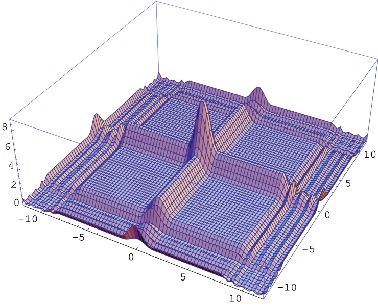
Figure 2. Polynomials ${\mathcal{P}}_{n}(\tau)$ for ${\boldsymbol{T}}\otimes{\boldsymbol{T}}$

For this purpose consider a trigonometric sum

(93) $${\mathcal{P}}(\tau_{1},\tau_{2})={\mathcal{P}}_{X}(\tau_{1})\,{\mathcal{P}}_{Y}(\tau_{2}),$$

(94) $${\mathcal{P}}_{X}(\tau_{1})=\frac{1}{\sqrt{q}}\sum_{y_{1}=0}^{q-1}e^{2\pi i\,\tau_{1}\omega_{X}(y_{1})},\qquad{\mathcal{P}}_{Y}(\tau_{2})=\frac{1}{\sqrt{q}}\sum_{y_{2}=0}^{q-1}e^{2\pi i\,\tau_{2}\omega_{Y}(y_{2})},$$

(95) $$\omega_{X}(y)=\omega_{Y}(y)=m\frac{q}{\beta^{2}}e^{\beta y/q}.$$

for a single step in the rank one construction (for simplicity we omit index $n$). Clearly, ${{\mathcal{P}}={\mathcal{P}}_{X}\otimes{\mathcal{P}}_{Y}}$ is just a tensor square of ${\mathcal{P}}_{X}$. We can represent ${\mathcal{P}}(\tau_{1},\tau_{2})$ in the following invariant form:

(96) $${\mathcal{P}}(\tau)=\frac{1}{q}\sum_{y_{1}=0}^{q-1}\sum_{y_{2}=0}^{q-1}e^{2\pi i\,\left\langle\tau,\,\omega(y)\right\rangle},$$

where ${\tau=(\tau_{1},\tau_{2})}$, ${y=(y_{1},y_{2})}$, and

(97) $$\left\langle\tau,\,\omega(y)\right\rangle=\tau_{1}\omega_{X}(y)+\tau_{2}\omega_{Y}(y),$$

(98) $$\omega(y)=\mu\frac{q}{\beta^{2}}(e^{\beta y_{1}/q},e^{\beta y_{2}/q}).$$

The following lemma directly follows from the one-dimensional one.

Lemma 30.

Consider a window in ${\mathbb{R}}^{2}$

(99) $$G=\bigl{(}(-b,-a)\cup(a,b)\bigr{)}\times\bigl{(}(-b,-a)\cup(a,b)\bigr{)}.$$

For any ${\varepsilon>0}$ we can find $L^{1}$-$\varepsilon$-flat sums in $G$ with a frequency function $\omega$ given by equation (98).

Following the terminology introduced by A. Danilenko (see [7]) we define our rank one action of the group ${\mathbb{R}}^{2}$ to be the rank one action given by a $(C,F)$-construction, where at $n$-th step of the construction: $C_{n}$ is an open set in ${\mathbb{R}}^{2}$ (analogue of the tower) and $F_{n}$ is a finite set. We set precisely

(100) $$C_{n}=(0,h_{n})\times(0,h_{n}),$$

(101) $$F_{n}=\bigl{\{}\bigl{(}\omega_{X}(y_{1},y_{2}),\omega_{Y}(y_{1},y_{2})\bigr{)}\colon\>(y_{1},y_{2})\in\{0,1,\dots,q_{n}-1\}^{\times 2}\bigr{\}}.$$

Lemma 31.

Given two functions $f_{1}$ and $f_{2}$ with zero mean the spectral measure ${\sigma_{f_{1}\otimes f_{2}}}$ with respect to the action ${\boldsymbol{T}}\otimes{\boldsymbol{T}}$ in the space ${H\otimes H}$ is absolutely continuous with respect to the Lebesgue measure. And the measure of maximal spectral type for ${\boldsymbol{T}}\otimes{\boldsymbol{T}}$ in the space $H^{(2)}$ of all functions with zero mean is equivalent to the sum of the Lebesgue measure and a singular measure with support on two coordinate axes,

(102) $$\sigma\sim\lambda+{\boldsymbol{\delta}}_{0}(\tau_{1})+{\boldsymbol{\delta}}_{0}(\tau_{2}).$$

The serious difference between dimension one and dimension ${d>2}$ is that the trivial subspace of constants in $L^{2}(X)$ produces a non-trivial subspace ${\{{\mathrm{const}}\}\times H}$ in $H^{(2)}$.

2.2. ${\mathbb{R}}^{d}$-actions with simple Lebesgue spectrum

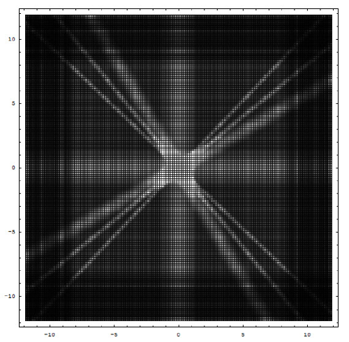
Figure 3. The structure of the Riesz product (density plot of $\prod_{n}{\mathcal{P}}_{n}(\tau)$ graph)

In the above discussion we have described the obstacle to simple Lebesgue spectrum for the frequency function ${\omega(y_{1},y_{2})=q\beta^{-2}(e^{\beta y_{1}/q},e^{\beta y_{2}/q})}$. Two components ${\boldsymbol{\delta}}(x_{1})$ and ${\boldsymbol{\delta}}(x_{2})$ appear in addition to Lebesgue component.

The idea of the next construction is to overcome this obstacle by choosing a sequence of different coordinate systems given by some linear transforms $\Psi_{n}$ in such a way that at any step of the construction the polynomials ${\mathcal{P}}_{n}(\tau)$ is rotated on the plane ${\mathbb{R}}^{2}$ according the transform $\Psi_{n}$,

(103) $$\Phi(\tau)=\prod_{n}{\mathcal{P}}_{n}(\Psi_{n}\tau)$$

and the “bad set”

(104) $$G_{n}^{c}={\mathbb{R}}^{2}\mathbin{\smallsetminus}G_{n}=({\mathbb{R}}^{2}\mathbin{\smallsetminus}[-b_{n},b_{n}]^{\times 2})\cup([-b_{n},b_{n}]\times[-a_{n},a_{n}])\cup([-a_{n},a_{n}]\times[-b_{n},b_{n}])$$

for the polynomial ${\mathcal{P}}_{n}(\tau)$ after applying $\Psi_{n}^{-1}$ is covered (in most part) by the windows

(105) $$\Psi_{n+1}^{-1}G_{n+1},\quad\Psi_{n+2}^{-1}G_{n+2},\quad\ldots$$

In other words, the part of the Riesz product $\prod_{k\><\>n}|{\mathcal{P}}_{k}(\tau)|^{2}$ which is not necessary flat is covered by the area of flatness of the polynomials ${\mathcal{P}}_{n+k}(\Psi_{n+k}\tau)$, ${k\geq 1}$, so that it becomes in a sense “frozen” for all further steps of the construction.

Remark that $G_{n}^{c}$ consists of the area outside a big square $[-b_{n},b_{n}]^{\times 2}$ and two thin rectangles

(106) $${\mathcal{F}}_{n}=([-b_{n},b_{n}]\times[-a_{n},a_{n}])\cup([-a_{n},a_{n}]\times[-b_{n},b_{n}])$$

located near coordinate axes (recall that ${b_{n}\to\infty}$ and ${a_{n}\to 0}$ as ${n\to\infty}$). We will find appropriate $\Psi_{n}$ to achieve the following effect:

(107) $$\max\{|\tau|\colon\>\tau\in\Psi_{n}^{-1}{\mathcal{F}}_{n}\cap\Psi_{n+k}^{-1}{\mathcal{F}}_{n+k}\}\to 0\quad\text{as $n\to\infty$},\qquad k\geq 1$$

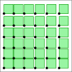
Figure 4. Illustration for the set $F_{1}$. The small squares are shifts of the set $C_{1}$, and the large bounding square is the set $C_{2}$. One can see that the distance between adjacent points slightly increases from the left to the right and from the bottom to the top.

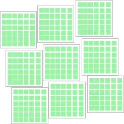
Figure 5. Illustration to construction 32, the second step.

Construction 32.

Assume that for each index $n$ a pair of basis vectors $\{\widehat{e}_{1}(n),\widehat{e}_{2}(n)\}$ is given such that

(108) $$|\widehat{e}_{1}(n)|=|\widehat{e}_{2}(n)|=1,$$

(109) $$\widehat{e}_{1}(n)=\Psi_{n}\begin{pmatrix}1\\ 0\end{pmatrix},\qquad\widehat{e}_{1}(n)=\Psi_{n}\begin{pmatrix}0\\ 1\end{pmatrix},$$

and let $\Psi_{n+1}=V_{n}\Psi_{n}$ be a small linear correction of $\Psi_{n}$ by a map $V_{n}$ to be defined later. Set

(110) $$F_{n}=\bigl{\{}\omega_{X,n}(y_{1})\,\widehat{e}_{1}(n)+\omega_{Y,n}(y_{2})\,\widehat{e}_{2}(n)\colon\>y\in\{0,\dots,q_{n}-1\}^{\times 2}\bigr{\}}$$

Let us define $\widehat{e}_{1}(n)$ and $\widehat{e}_{2}(n)$ as follows. Imagine that everuthing is consider in the coordinate system connected to the original one via the transform $\Psi_{n}$. In this coordinate system $\widehat{e}_{j}(n)$ becomes $(1,0)$ and $(0,1)$ and $\Psi_{n}^{-1}F_{n}$ is exactly the non-perturbed set $F_{n}$ comming from the beginning example of ${\boldsymbol{T}}\otimes{\boldsymbol{T}}$. It looks like a rectangular grid ${F_{n}^{(1)}\times F_{n}^{(1)}}$ so that the adjacent points in this set connected by a vector ${v\approx(h_{n},0)}$ or ${v\approx(0,h_{n})}$. Now let us set

(111) $$h_{n+1}\,\widehat{e}_{1}(n+1)=\ell_{n}\widehat{e}_{1}(n)+\xi_{n}\ell_{n}e_{2}(n),\quad h_{n+1}\,\widehat{e}_{2}(n+1)=-\xi_{n}\ell_{n}e_{2}(n)+\ell_{n}e_{1}(n),$$

(112) $$\ell_{n}=q_{n}h_{n}e^{\beta_{n}}.$$

(Notice that for the original non-perturbed construction of ${\boldsymbol{T}}\otimes{\boldsymbol{T}}$ we would have ${\xi_{n}=0}$.)

Thus, one can get the following representation for the elementary rotation on each step:

(113) $$V_{n}=\begin{pmatrix}1&-\xi_{n}\\ \xi_{n}&1\end{pmatrix}.$$

Such kind of cunstruction in the context of ${\mathbb{Z}}$-actions was used by V. Ryzhikov in [24]. The spectral measure $\sigma_{f}$ can be represented in a form of a Riesz product, which is formal so far, and our purpose is to prove its convergence:

(114) $$\sigma_{n}=|f_{(n_{0})}|^{2}\,\prod_{n=n_{0}}^{\infty}|{\mathcal{P}}_{n}(\tau)|^{2}\,d\tau,\qquad{\mathcal{P}}_{n}=\frac{1}{q_{n}}\,\widehat{\bf 1}_{F_{n}},$$

where

(115) $${\bf 1}_{F_{n}}=\sum_{t\>\in\>F_{n}}{\boldsymbol{\delta}}_{t}=\sum_{y_{1}=0}^{q_{n}-1}\sum_{y_{2}=0}^{q_{n}-1}{\boldsymbol{\delta}}_{\omega(y_{1},y_{2})\Psi^{-1}_{n}},$$

According to this modification applied to $F_{n}$ let us define $C_{n}$ to be the open set $\Psi_{n}((0,h_{n})\times(0,h_{n}))$.

Theorem 33.

The rank one ${\mathbb{R}}^{2}$-action built in construction 32 has simple Lebesgue spectrum if $q_{n}$ go to infinity sufficiently fast.

Proof.

It is enough to establish that $\sigma_{f}$ is absolutely continuous for any $f$ constant on the levels of the $n_{0}$’th tower. If we compare this action with the construction of rank one flow described above all the points on the plane can be classified to the following three groups:

• points covered by many (more than one) sets ${\mathcal{F}}_{n}$, where flatness of ${\mathcal{P}}_{n}(\tau)$ cannot be controlled;

• points containing infinitely many ${\mathcal{F}}_{n}$ entering its arbitrary small boundary;

• points with a boundary free from points from ${\mathcal{F}}_{n}$ starting from some $n^{*}$;

Notice that the case (b) is not present for the flow, but in the case of the ${\mathbb{R}}^{2}$-action the case (b) is observed on the limit set of ${\mathcal{F}}_{n}$ which is non-empty and consists of two limit lines crossing at zero (see figure 3). It can be easily seen that the intersection of ${\mathcal{F}}_{n}$ and ${\mathcal{F}}_{m}$ can be fit in a ball of radius

(116) $$r_{n,m}=O\!\left(\frac{a_{n}+a_{m}}{\varphi_{n,m}}\right),$$

where $a_{n}$ is the thickness of the rectangular strips in ${\mathcal{F}}_{n}$, and $\varphi_{n,m}$ is the angle between them,

(117) $$\varphi_{n,m}\sim\xi_{n}+\xi_{n+1}+\ldots+\xi_{m-1}\leq\sum_{k\geq n}\xi_{k}$$

if ${n<m}$. Since $\xi_{n}$ are fixed in advance, before we construct the sequence of flat polynomials, we have to require the following condition:

(118) $$a_{n}\ll\sum_{k\geq n}\xi_{k}$$

to ensure that all these intersections collapses to the zero point, so that we can apply the same arguments like in the case of rank one flow and see that atom at zero in the limit distribution prohibited by the ergodicity of the actions.

At the same time, case (b) appear only in the multidimensional case and to complete the proof we have to use the following lemma on the polynomials used in the construction (see lemma 7).

Lemma 34.

A flat polynomial ${\mathcal{P}}(\tau_{1})$ on ${\mathbb{R}}$ build for the function

(119) $$\omega(y)=M\frac{q}{\beta^{2}}e^{\beta y/q}.$$

can be estimated near zero as follows:

(120) $$\|{\mathcal{P}}\|_{L^{1}(-a,a)}=O\!\left(\frac{\log aq}{\sqrt{q}}\right),\qquad a<1.$$

Using this lemma one can see that for any small neighbourhood $U_{0}$ of a limit line the intersections $U_{0}\cap{\mathcal{F}}_{n}$ become disjoint starting at some indedx $n_{1}$ and

(121) $$\sum_{n\geq n_{1}}\|{\mathcal{P}}_{n}|_{U_{0}\cap{\mathcal{F}}_{n}}\|_{1}<\infty.$$

This calculation cannot be applied to the case (a), since the polynomials ${\mathcal{P}}_{n}(\tau)$ are multiplied and if we loose disjointness of ${\mathcal{F}}_{n}$ it will be impossible to control the Riesz product behaviour.

The case (c) corresponds to the area of flatness. ∎

We have considered only the case of rank one ${\mathbb{R}}^{2}$-actions and the same effects remain for ${\mathbb{R}}^{d}$-actions. Thus, the existence of rank one actions with Lebesgue spectrum is established using the same technique.

The author is very greatly to El. Houcein El Abdalaoui, Bassam Fayad, Mariusz Lemanczyk and Jean-Paul Thouvenot for the deep and helpful discussions concerning the first part of this paper.

References

- [1] El H. El Abdalaoui, La singularité mutuelle presque sûre du spectre des transformatioys d’ornstein, Isr. . .J. . .Math. 112 (1999), 135–155.
- [2] by same author, On the spectrum of the powers of ornstein transformations, Special issue on Ergodic theory and harmonic analysis. Shankyā, ser. . .A 62 (2000), no. 3, 291–306.
- [3] El H. El Abdalaoui, F. Parreau, and A.A. Prikhod’ko, A new class of ornstein transformations with singular spectrum, Annales de l’Institut Henri Poincare (B) Probability and Statistics 42 (2006), no. 6, 671–681.
- [4] O.N. Ageev, The homogeneous spectrum problem in ergodic theory, Invent. Math. 160 (2005), no. 2.
- [5] D.V. Anosov, On spectral multiplicity in ergodic theory, (2003).
- [6] J. Bourgain, On the spectral type of ornstein class one transformations, Isr. . .J. . .Math. 84 (1993), 53–63.
- [7] A.I. Danilenko, Funny rank-one weak mixing for nonsingular abelian actions, Isr. J. Math. 121 (2001), 29–54.
- [8] A.I. Danilenko and V.V. Ryzhikov, Mixing constructions with infinite invariant measure and spectral multiplicities, preprint, arxiv: 0908.1643v2, (2010), 1 –21.
- [9] T. Downarowicz and Y. Lacroix, Merit factors and morse sequences, Theoretical Computer Science archive 209 (1998), no. 1–2, 377–387.
- [10] T. Erdelyi, Polynomials with littlewood-type coefficient constraints, Approximation Theory X: Abstract and Classical Analysis, Charles K. Chui, Larry L. Schumaker, and Joachim Stockler (Eds.) (2002), 153–196.
- [11] M. Guenais, Morse cocycles and simple lebesgue spectrum, Ergodic Theory and Dynamical Systems 19:2 (1999), 437–446.
- [12] E. Janvresse, T. De La Rue, and V. Ryzhikov, Around king’s rank-one theorems: Flows and -actions, preprint, arxiv: 1108.2767v1.
- [13] J.-P. Kahane, Sur les polynômes à coefficients unimodulaires, Bull. . .London Math. . .Soc. 12 (1980), 321–342.
- [14] A. Katok and M. Lemanczyk, Some new cases of realization of spectral multiplicity function for ergodic transformations (special volume dedicated to m. misiurewicz), Fundamenta Math. 206 (2009), 185–215.
- [15] A.A. Kirillov, Dynamical systems, factors and representations of groups, Russian Math. Surveys 22 (1967), no. 5, 63–75.
- [16] I.P. Kornfel’d, Ya.G. Sinaĭ, and S.V. Fomin, Ergodic theory, Nauka, Moscow / Springer–Verlag, Berlin–Heidelberg–New York, 1982.
- [17] M. Lemańczyk, Spectral theory of dynamical systems, encyclopedia of complexity and system science, Springer Verlag, 2009.
- [18] J.E. Littlewood, On polynomials, , , , J. London Math., Soc. 41 (1966), 367–376.
- [19] D.S. Ornstein, On the root problem in ergodic theory, Proc. . .6th Berkley Sympos. . .Math. . .Statist. . .Probab., Univ. . .Calif. 2 (1970), 347–356.
- [20] A.A. Prikhod’ko, On ergodic properties of “iceberg” transformations. I: approximation and spectral multiplicity, preprint, arxiv:1002.2808v1.
- [21] by same author, Stochastic constructions of flows of rank , Sb. . .Math. 192 (2001), no. 12, 1799–1828.
- [22] by same author, On flat trigonometric sums and flows with simple lebesgue spectrum, preprint, arxiv:1002.2808v1, (2010), 1–18.
- [23] V.A. Rokhlin, On the fundamental ideas of measure theory, Mat. Sb. (N.S.) 25 (1949), no. 67.
- [24] V.V. Ryzhikov, The -free rokhlin–halmos property is not satisfied for the actions of the group , Mat. Zametki 44 (1988), no. 2, 208–215.
- [25] R. Salem, On some singular monotonic functions which are strictly increasing, Trans. Amer. Soc. Math. 53 (1943), no. 3, 427 –439.
- [26] by same author, Sets of uniqueness and sets of multiplicity, Trans. Amer. Soc. Math. 54 (1943), 218 –228.
- [27] S.M. Ulam, A collection of mathematical problems. interscience tracts in pure and applied mathematics, no. 8, New York, Interscience, 1960.
- [28] M. Weiss, On hardy-littlewood series, Transactions of the American Mathematical Society 91 (1959), no. 3, 470–479.