The Average Likelihood Ratio for Large-scale Multiple Testing and Detecting Sparse Mixtures

Abstract

Large-scale multiple testing problems require the simultaneous assessment of many p-values. This paper compares several methods to assess the evidence in multiple binomial counts of p-values: the maximum of the binomial counts after standardization (the ‘higher-criticism statistic’), the maximum of the binomial counts after a log-likelihood ratio transformation (the ‘Berk-Jones statistic’), and a newly introduced average of the binomial counts after a likelihood ratio transformation. Simulations show that the higher criticism statistic has a superior performance to the Berk-Jones statistic in the case of very sparse alternatives (sparsity coefficient $\beta\gtrapprox 0.75$), while the situation is reversed for $\beta\lessapprox 0.75$. The average likelihood ratio is found to combine the favorable performance of higher criticism in the very sparse case with that of the Berk-Jones statistic in the less sparse case and thus appears to dominate both statistics. Some asymptotic optimality theory is considered but found to set in too slowly to illuminate the above findings, at least for sample sizes up to one million. In contrast, asymptotic approximations to the critical values of the Berk-Jones statistic that have been developed by Wellner and Koltchinskii (2003) and Jager and Wellner (2007) are found to give surprisingly accurate approximations even for quite small sample sizes.

t1Work supported by NSF grant DMS-1007722

1 Introduction

This paper is concerned with the following mixture problem: One observes $X_{1},\ldots,X_{n}$ i.i.d. $F$ and one wants to test

$$H_{0}:\ F=\Phi,\ \ \ \mbox{ the standard normal distribution function}$$

versus

$$H_{1}:\ F=(1-\epsilon)\Phi+\epsilon\Phi(\cdot-\mu)\ \ \ \ \mbox{ for some }\epsilon\in(0,1),\mu>0.$$

Interest in this prototypical setting derives from a number of applications that involve large-scale multiple testing, see e.g. Donoho and Jin (2004). In the case where the proportion of nonzero means is small, $\epsilon=\epsilon_{n}=n^{-\beta}$, for $\beta\in(\frac{1}{2},1)$, there is the following result: Parametrize $\mu=\mu_{n}=\sqrt{2r\log n}$ for $r\in(0,1)$ and define the detection boundary

$$\rho^{*}(\beta)=\begin{cases}\beta-\frac{1}{2}&\text{if $\frac{1}{2}<\beta\leq\frac{3}{4}$},\\ (1-\sqrt{1-\beta})^{2}&\text{if $\frac{3}{4}<\beta<1$}.\end{cases}$$

If $r<\rho^{*}(\beta)$, then it is impossible to detect the presence of the nonzero means $\mu_{n}$: Any test with asymptotic level $\alpha\in(0,1)$ can only have trivial asymptotic power $\alpha$. On the other hand, if $r>\rho^{*}(\beta)$, then the likelihood ratio test (which requires the knowledge of $\beta$ and $r$) at asymptotic level $\alpha$ will have asymptotic power 1, see Ingster (1997,1998) and Jin (2004). But $\beta$ and $r$ are unknown, so direct application the likelihood ratio test is not possible. Jin (2004) and Donoho and Jin (2004) propose to employ the higher criticism statistic

$$\mbox{HC}_{n}^{*}\ =\ \max_{1\leq i\leq n/2}\sqrt{n}\Bigl{(}i/n-p_{(i)}\Bigr{)}/\sqrt{p_{(i)}(1-p_{(i)})},$$

where $p_{i}={\rm I\!P}(N(0,1)>X_{i})$ is the p-value of $X_{i}$, and they show that $\mbox{HC}_{n}^{*}$ also attains the optimal detection boundary, i.e. $\mbox{HC}_{n}^{*}$ has asymptotic power 1 for all $\beta\in(\frac{1}{2},1)$ and $r>\rho^{*}(\beta)$. Note that $\mbox{HC}_{n}^{*}$ does not require the knowledge of $\beta$ and $r$.

2 Combining the evidence of multiple binomial counts

Denote by $F_{n}$ the empirical distribution function of the p-values: $F_{n}(t):=\frac{1}{n}\sum_{i=1}^{n}1(p_{i}\leq t)$. Then one sees that

$$\mbox{HC}_{n}^{*}=\max_{t\in\{p_{(1)},\ldots,p_{(n/2)}\}}\sqrt{n}\frac{F_{n}(t)-t}{\sqrt{t(1-t)}}.$$ (1)

Under the null hypothesis, the p-values $p_{i}$ are an i.i.d. sample from $U[0,1]$. Thus the quantity $\sqrt{n}\frac{F_{n}(t)-t}{\sqrt{t(1-t)}}$ is the standardized count of p-values that fall in the interval $(0,t]$, and so $\mbox{HC}_{n}^{*}$ looks for an excessive number of p-values in the intervals $(0,t]$ for $t\in(0,\frac{1}{2}]$ by considering the maximum of these standardized binomial counts over the intervals $(0,p_{(i)}]$ for $i=1,\ldots,n/2$.

While a standardized binomial random variable is a classical example to illustrate the convergence to a normal distribution, it is important to keep in mind that its long tail is not any more subgaussian: As the success probability moves from $\frac{1}{2}$ to $0$, the long tail becomes increasingly heavy, see Shorack and Wellner (1986,Ch.11.1). In fact, the first several terms in $\mbox{HC}_{n}^{*}$ even have heavy algebraic tails, as can be seen from an argument similar to Sec. 3 in Donoho and Jin (2004). Since the distribution of the $\max$ depends sensitively on the tails, this means that standardizing the counts does not guarantee that all counts are treated equally. Rather, $\mbox{HC}_{n}^{*}$ gives increasingly more weight to counts with smaller index $i$. This raises the question what effect this has on the performance of $\mbox{HC}_{n}^{*}$.

To investigate this issue, we can compare the performance of $\mbox{HC}_{n}^{*}$ with a statistic that standardizes the binomial counts differently to avoid unequal and heavy tails. Such a standardization is given by the log-likelihood ratio transformation. Define

$$logLR_{n}(t)=\begin{cases}nF_{n}(t)\log\frac{F_{n}(t)}{t}+n(1-F_{n}(t))\log\frac{1-F_{n}(t)}{1-t}&\text{if $0<t<F_{n}(t)$},\\ 0&\text{otherwise}.\end{cases}$$

$logLR_{n}(t)$ is the one-sided log-likelihood ratio statistic for testing whether the parameter of the binomial count $nF_{n}(t)$ equals $t$ vs. whether it is larger than $t$. The log-likelihood ratio transformation possesses the important property that it produces clean subexponential tails under the null hypothesis, no matter what the binomial parameter $t$. This fact is implicit in the proof of the Chernoff-Hoeffding theorem, see Hoeffding (1963). One can now proceed as with $\mbox{HC}_{n}^{*}$ and take the maximum of the thus standardized binomial counts over the random intervals $(0,p_{(i)}]$. This essentially yields a statistic proposed by Berk and Jones (1979):

$$\mbox{BJ}_{n}^{+}\ =\ \max_{1\leq i\leq n/2}logLR_{n,i},$$

where $logLR_{n,i}:=logLR_{n}(p_{(i)})=(i\log\frac{i}{np_{(i)}}+(n-i)\log\frac{1-i/n}{1-p_{(i)}})1(p_{(i)}<\frac{i}{n})$. $\mbox{BJ}_{n}^{+}$ was shown by Donoho and Jin (2004) to also attain the optimal detection boundary. Both $\mbox{HC}_{n}^{*}$ and $\mbox{BJ}_{n}^{+}$ are special cases of a family of goodness-of-fit tests based on $\phi$-divergences that are introduced and studied by Jager and Wellner (2007).

We compare the power of $\mbox{HC}_{n}^{*}$ and $\mbox{BJ}_{n}^{+}$ against alternatives $\mu_{n}=\sqrt{2r\log n}$ with $r=r(\beta)=1.2\rho^{*}(\beta)+0.1$ for ten equally spaced values of $\beta$ between 0.5 and 1. The significance level was set to 5% by estimating the exact finite sample critical values of $\mbox{HC}_{n}^{*}$ and $\mbox{BJ}_{n}^{+}$ with $10^{5}$ simulations. The power of $\mbox{HC}_{n}^{*}$ and $\mbox{BJ}_{n}^{+}$ was then simulated with $10^{4}$ simulations. The left plot in Figure 1 shows the resulting power values for sample size $n=10^{4}$, the right plot for sample size $n=10^{6}$. One sees that $\mbox{HC}_{n}^{*}$ has a better detection performance in the very sparse case $\beta\gtrapprox\frac{3}{4}$, while $\mbox{BJ}_{n}^{+}$ has a better performance for smaller $\beta$.

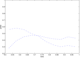
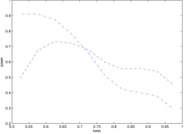
Figure 1: Power of $\mbox{HC}_{n}^{*}$ (dashed) and $\mbox{BJ}_{n}^{+}$ (dash-dot) as a function of the sparsity parameter $\beta$. The left plot shows power for sample size $n=10^{4}$, the right plot for $n=10^{6}$.

The preceding discussion suggests the following explanation of this result: Donoho and Jin (2004) observed that for $\beta\in[\frac{3}{4},1)$ the strongest evidence against $H_{0}$ is found near the maximum of the observations, i.e. at the smallest p-values. Since $\mbox{HC}_{n}^{*}$ gives more weight to smaller p-values compared to $\mbox{BJ}_{n}^{+}$, $\mbox{HC}_{n}^{*}$ will have more power. But when $\beta\in(\frac{1}{2},\frac{3}{4})$, then the most informative place to look is at larger p-values, i.e. one needs to examine the count of p-values in the interval $(0,t]$ for certain $t\in(0,1)$. Since $\mbox{HC}_{n}^{*}$ gives less weight to the evidence in those intervals, it suffers a performance penalty in this case.

The simulation study also confirms the cautionary remarks in Donoho and Jin (2004) about the sample size required for the above asymptotic optimality theory to adequately assess the performance of statistical procedures. Both $\mbox{HC}_{n}^{*}$ and $\mbox{BJ}_{n}^{+}$ attain the optimal detection boundary, i.e. have asymptotic power 1 against the alternatives considered in the above simulation study. But even for a sample size of one million, their detection power is quite small for a large range of $\beta$ values. Moreover, the difference in power between these two optimal procedures is larger than the gain in power obtained by increasing the sample size 100fold from $n=10^{4}$ to $n=10^{6}$. Thus it appears that the asymptotic optimality theory sets in too slowly to be informative for sample sizes up to at least a million, and it seems prudent to instead assess the performance of such procedures primarily via simulation studies.

The difference in performance between $\mbox{HC}_{n}^{*}$ and $\mbox{BJ}_{n}^{+}$ for various $\beta$ raises the question whether this difference represents an unavoidable trade-off, or whether it is possible to improve on this overall performance. If a better performance is possible, how should one go about developing a better test?

3 The average likelihood ratio statistic

A promising approach to obtain good power uniformly in $\beta$ is a minimax test, which is typically constructed as a Bayes solution with respect to a least favorable prior, see Lehmann and Romano (2005,Ch.8.1). But in the context at hand, such a construction appears to be involved since it requires the specification a multivariate prior over an appropriate set of alternative distributions.

Instead we proceed as follows: Suppose we start with an noninformative uniform prior for the parameter $\beta$ on $(\frac{1}{2},1)$. Given $\beta$, we can use knowledge about the problem to construct an appropriate conditional test: Donoho and Jin (2004) observe that for $\beta\in[\frac{3}{4},1)$ the most promising approach is essentially to look at the smallest p-value. Thus we put prior probability $\frac{1}{2}$ on the likelihood ratio test over the interval $(0,p_{(1)}]$. For $\beta\in(\frac{1}{2},\frac{3}{4})$, the most promising interval to detect alternatives with $r$ close to the detection boundary $\rho^{*}(\beta)=\beta-\frac{1}{2}$ is the interval $(0,n^{-4r}]$. Thus given such a $\beta$, we will employ the likelihood ratio test on the interval $(0,t]$ with $t=n^{-4(\beta-\frac{1}{2})}$. If $\beta\sim U(\frac{1}{2},\frac{3}{4})$, then $t=n^{-4(\beta-\frac{1}{2})}$ has density proportional to $\frac{1}{t}$ on $(\frac{1}{n},1)$. Approximating the resulting posterior integral with the corresponding weighted sum of the $p_{(i)}$ and observing that the normalizing factor of the weights is $\sum_{i=2}^{n/2}\frac{1}{i}\approx\log(n/3)$ yields the average likelihood ratio

$$\mbox{ALR}_{n}\ =\ \frac{1}{2}LR_{n,1}+\frac{1}{2}\sum_{i=2}^{n/2}\frac{1}{i\log(n/3)}LR_{n,i}$$

where

$$LR_{n,i}=\begin{cases}\Bigl{(}\frac{i}{np_{(i)}}\Bigr{)}^{i}\Bigl{(}\frac{1-\frac{i}{n}}{1-p_{(i)}}\Bigr{)}^{n-i}&\text{if $p_{(i)}<\frac{i}{n}$},\\ 1&\text{otherwise}.\end{cases}$$

Thus $LR_{n,i}$ is the one-sided likelihood ratio statistic for testing whether the parameter of the binomial count on $(0,t]$ equals $t$, evaluated at $t=p_{(i)}$.

Theorem.

$\mbox{ALR}_{n}$ attains the optimal detection boundary.

For a proof, note that it was shown in Donoho and Jin (2004) that with probability converging to 1 there exists an index $i\in\{1,\ldots,n/2\}$ such that $logLR_{n,i}\gtrapprox n^{\kappa}$, where $\kappa=\kappa(\beta,r)>0$. Hence $\mbox{BJ}_{n}^{+}$ (and $\mbox{HC}_{n}^{*}$) grow algebraically fast under the alternative. Now $LR_{n,i}=\exp(logLR_{n,i})\gtrapprox\exp(n^{\kappa})$. Thus $\mbox{ALR}_{n}$ grows exponentially fast. Some informal arguments given below suggest that $\mbox{ALR}_{n}$ may have a limiting distribution under $H_{0}$, but to complete the proof in a rigorous way it is enough to employ the upper bound $\mbox{ALR}_{n}\leq 2\exp(\mbox{BJ}_{n}^{+})$ together with $\mbox{BJ}_{n}^{+}/\log\log n\stackrel{{\scriptstyle p}}{{\rightarrow}}1$ under $H_{0}$, see Jager and Wellner (2007,Thm.3.1). $\Box$

The exponential increase of $\mbox{ALR}_{n}$ has to be taken with a grain of salt. Depending on $\beta$ and $r$, the constant $\kappa(\beta,r)$ may be close to zero. Then an enormous $n$ is required for $LR_{n,i}$ to overcome the divisor $i\log(n/3)$ if $i\geq 2$. Of course, the same calamity befalls $\mbox{BJ}_{n}^{+}$ and $\mbox{HC}_{n}^{*}$, where the polynomial $n^{\kappa}$ needs to overcome a critical value of order $\log\log n$. This appears to be one of the reasons why the asymptotic theory is so slow to take hold.

As discussed above, it is therefore preferrable to evaluate the performance of $\mbox{ALR}_{n}$ with a simulation study. Figure 2 compares the power of $\mbox{ALR}_{n}$, $\mbox{HC}_{n}^{*}$, and $\mbox{BJ}_{n}^{+}$ in the same setting that was considered in section 2.

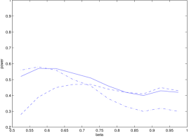
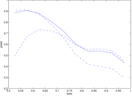
Figure 2: Power of $\mbox{ALR}_{n}$ (solid), $\mbox{HC}_{n}^{*}$ (dashed) and $\mbox{BJ}_{n}^{+}$ (dash-dot) as a function of the sparsity parameter $\beta$. The left plot shows power for sample size $n=10^{4}$, the right plot for $n=10^{6}$.

One sees that $\mbox{ALR}_{n}$ combines the good performance of $\mbox{HC}_{n}^{*}$ at larger $\beta$ with the good performance of $\mbox{BJ}_{n}^{+}$ at smaller $\beta$ and thus results in a test that appears to dominate both $\mbox{HC}_{n}^{*}$ and $\mbox{BJ}_{n}^{+}$.

To avoid numerical difficulties when $n$ is large, it is advisable to rewrite $LR_{n,i}=\exp(logLR_{n,i})$ with $logLR_{n,i}$ given in section 2. As above, the simulation study used a size of 5% for all three tests by estimating the exact finite sample critical values with $10^{5}$ simulations. Since such a simulation may not be practical for larger samples, it is of interest to explore whether reasonably accurate asymptotic approximations are available.

4 Asymptotic approximations for the null distributions

A first attempt to derive a simple large sample approximation for the critical values of $\mbox{HC}_{n}^{*}$ and $\mbox{BJ}_{n}^{+}$ can be based on $\mbox{HC}_{n}^{*}/\sqrt{2\log\log n}\stackrel{{\scriptstyle P}}{{\rightarrow}}1$ and $\mbox{BJ}_{n}^{+}/\log\log n\stackrel{{\scriptstyle P}}{{\rightarrow}}1$, which follows e.g. from Jager and Wellner (2007,Thm.3.1). The significance levels obtained by using the resulting thresholds $\sqrt{2\log\log n}$ and $\log\log n$ for $\mbox{HC}_{n}^{*}$ and $\mbox{BJ}_{n}^{+}$, respectively, are listed under ‘thresh’ in Table 1. One sees that the resulting size of the tests is very large even for $n=10^{6}$.

A more refined approximation can be derived from results about the convergence to an extreme value distribution. In the case of $\mbox{HC}_{n}^{*}$, this result follows from Jaeschke (1979) and Eicker (1979), see also Shorack and Wellner (1986, Ch.16). In the case of $\mbox{BJ}_{n}^{+}$ a proof was sketched in Berk and Jones (1979). Wellner and Koltchinskii (2003) note an apparent error in that sketch and give a rigorous proof. See also Jager and Wellner (2007,Thm.3.1) for a unified treatment of $\mbox{HC}_{n}^{*}$ and $BJ$. The latter theorem establishes convergence of two-sided versions of $\mbox{BJ}_{n}^{+}$ and $\frac{1}{2}(\mbox{HC}_{n}^{*})^{2}$, after centering, to an extreme value distribution with distribution function $E_{v}^{4}(x)=\exp(-4\exp(-x))$. As remarked in Shorack and Wellner (1986,p.600), the two one sided versions as well as the two halves ($i\lessgtr n/2$) are asymptotically independent. Therefore the pertinent limit for $\mbox{HC}_{n}^{*}$ and $\mbox{BJ}_{n}^{+}$ considered here should be $E_{v}^{1}$. The resulting approximation for the level $\alpha$ critical value for $\mbox{BJ}_{n}^{+}$ is

$$q_{\alpha}:=\log\log n+\frac{1}{2}\log\log\log n-\frac{1}{2}\log(4\pi)-\log(-\log(1-\alpha)),$$ (2)

and the corresponding approximation for $\mbox{HC}_{n}^{*}$ is $\sqrt{2q_{\alpha}}$. It is known that convergence to an extreme value distribution is typically extremely slow, see Hall (1979). Thus there would seem to be little hope that the above approximation is useful for moderate sample sizes, in particular since it involves a doubly-iterated (!) logarithm. But surprisingly, the simulation study in Table 1 shows that the above approximation (labelled ‘EVI’) is quite good for $\mbox{BJ}_{n}^{+}$ even for sample sizes as small as $n=100$. This appears to be another benefit of the clean exponential tails resulting from the log-likelihood ratio transformation. Unfortunately, the approximation does not work well for $\mbox{HC}_{n}^{*}$, where it yields very anti-conservative results.

Wellner and Koltchinskii (2003) suggest a further improvement for the approximation to $\mbox{BJ}_{n}^{+}$ by using the centering $c_{n}^{2}/(2b_{n}^{2})$ with $c_{n}=2\log\log n+\frac{1}{2}\log\log\log n-\frac{1}{2}\log(4\pi)$ and $b_{n}^{2}=2\log\log n$ in place of the first three terms on the right hand side of (2). The results of this approximation are labelled ‘EVII’ in Table 1 and show a further improvement for $\mbox{BJ}_{n}^{+}$, but still not a useful outcome for $\mbox{HC}_{n}^{*}$. This is presumably due to the heavy binomial tails which are not taken care of by the standardization in $\mbox{HC}_{n}^{*}$.

In connection to this it is worth pointing out that a key argument in proving the above limit theorems is to show that with high probability the first $\log^{5}n$ terms in $\mbox{HC}_{n}^{*}$ and $\mbox{BJ}_{n}^{+}$ do not contribute to the maximum, and that for the remaining terms a strong approximation with a Brownian bridge is applicable. In particular, this means that asymptotically the heavy binomial tails don’t matter, and that the maximum will not be attained at the first few terms. But as shown by the simulations above and elsewhere, such as in Donoho and Jin (2004), this is certainly not the case for sample sizes of up to at least $n=10^{6}$, which is the largest sample size we could explore in a reasonable amount of time. As remarked in Wellner (2006,p.43) concerning the applicability of the asymptotic results, one needs $n>1010388\approx 10^{6}$ just to get $\log^{5}n<n/2$.

Calibration	thresh		EVI				EVII
Statistic	$\mbox{HC}_{n}^{*}$	$\mbox{BJ}_{n}^{+}$	$\mbox{HC}_{n}^{*}$		$\mbox{BJ}_{n}^{+}$		$\mbox{HC}_{n}^{*}$		$\mbox{BJ}_{n}^{+}$
Nominal level in %	-	-	5	10	5	10	5	10	5	10
$n=10^{2}$	44.7	34.7	20.8	27.2	7.2	13.4	19.6	25.3	6.2	11.4
$10^{3}$	45.0	34.0	20.0	26.2	6.7	12.3	19.1	25.1	6.1	11.2
$10^{4}$	45.7	34.4	19.2	25.2	6.4	11.7	18.6	24.3	5.9	10.9
$10^{5}$	45.6	34.4	18.4	24.4	6.2	11.3	17.9	23.7	5.9	10.7
$10^{6}$	46.0	34.9	18.0	23.9	6.2	11.4	17.6	23.3	5.9	10.8

Table 1: Finite sample significance levels (in %) of $\mbox{HC}_{n}^{*}$ and $\mbox{BJ}_{n}^{+}$ for various asymptotic approximations to critical values. Based on $10^{5}$ simulations.

Next we consider $\mbox{ALR}_{n}$ and write

$$logLR_{n,1} = \Bigl{[}\log\frac{1}{np_{(1)}}+(n-1)\log\frac{1-1/n}{1-p_{(1)}}\Bigr{]}1(p_{(1)}<1/n)$$

$$= \Bigl{[}-\log\Bigl{(}np_{(1)}\Bigl{(}1-\frac{np_{(1)}}{n}\Bigr{)}^{n}\Bigr{)}+\log(1-p_{(1)})+(n-1)\log(1-1/n)\Bigr{]}1(np_{(1)}<1).$$

Recall that under $H_{0}$ we can use the representation $p_{(1)}\stackrel{{\scriptstyle d}}{{=}}E_{1}/(E_{1}+\ldots+E_{n+1})$, where $\{E_{i}\}$ is an infinite sequence of i.i.d. Exp(1) random variables, see Shorack and Wellner (1986,p.335). Thus $logLR_{n,1}$ has the same distribution as a random variable that converges a.s. to $(-\log E_{1}+E_{1}-1)1(E_{1}<1)$ by the strong law. Hence

$$LR_{n,1}\stackrel{{\scriptstyle d}}{{\rightarrow}}\Bigl{(}\frac{\exp(E_{1})}{eE_{1}}\Bigr{)}^{1(E_{1}<1)}.$$ (3)

Next, set ${\cal I}_{n}:=\{i:p_{(i)}\leq\log^{5}n/n\}$. Using (A.4) in Donoho and Jin (2004) and (26) on p.602 of Shorack and Wellner (1986), we get

$$\max_{i\in{\cal I}_{n}}\ logLR_{n,i}\ \leq\ \max_{i\in{\cal I}_{n}}\frac{\Bigl{(}\frac{i}{n}-p_{(i)}\Bigr{)}^{2}}{2p_{(i)}(1-p_{(i)})}\ =\ o_{p}(\log\log n).$$

Hence on the event ${\cal A}_{n}:=\{\#{\cal I}_{n}\leq 2\log^{5}n\}$:

$$\sum_{i\in{\cal I}_{n}}\frac{1}{i\log(n/3)}LR_{i}\ \leq\ \exp\Bigl{(}(o_{p}(\log\log n)\Bigr{)}\frac{2\log\log n}{\log(n/3)}\ =\ o_{p}(1),$$

and ${\rm I\!P}({\cal A}_{n}^{c})={\rm I\!P}(\mbox{bin}(n,\log^{5}n/n)>2\log^{5}n)\rightarrow 0$ by Chebychev.

For $p_{(i)}>\log^{5}n/n$ one can proceed as in the proof of Thm. 3.1 in Jager and Wellner (2007), see also the proof of Thm. 1.1 in Wellner and Koltchinskii (2003), and as on p.601 of Shorack and Wellner (1986) and first approximate the log-likelihood ratio process by the square of the normalized empirical process and then by the square of a normalized Brownian Bridge. This suggests that

$$\sum_{i=2}^{n/2}\frac{1}{i\log(n/3)}LR_{n,1}\approx L_{n}:=\frac{1}{\log n}\int_{1/n}^{1/2}\frac{1}{t}\exp\Bigl{(}\frac{{B^{+}}^{2}(t)}{2t(1-t)}\Bigr{)}dt.$$

It is not clear whether $L_{n}$ has a finite limit distribution. Simulations show that the quantiles of $L_{n}$ increase very slowly as $n$ increases from $10^{2}$ to $10^{6}$. Formally applying l’Hôpital’s rule gives $\lim_{n\rightarrow\infty}L_{n}=\lim_{n\rightarrow\infty}\exp\Bigl{(}\frac{{B^{+}}^{2}(1/n)}{2/n(1-1/n)}\Bigr{)}$. Since $\exp\Bigl{(}\frac{{B^{+}}^{2}(1/n)}{2/n(1-1/n)}\Bigr{)}\stackrel{{\scriptstyle d}}{{=}}\exp(\frac{1}{2}{Z^{+}}^{2})$ with $Z\sim$N(0,1), a conjecture for the limit law of $\mbox{ALR}_{n}$ would be

$$\frac{1}{2}\Bigl{(}\frac{\exp(E_{1})}{eE_{1}}\Bigr{)}^{1(E_{1}<1)}+\frac{1}{2}\exp(\frac{1}{2}{Z^{+}}^{2}).$$ (4)

This expression reflects the fact that the beta distribution of the first order statistic behaves like an exponential distribution, while sufficiently larger order statistics possess a beta distribution that is closer to a normal. Of course, l’Hôpital’s rule is not applicable since $\lim_{n\rightarrow\infty}\exp\Bigl{(}\frac{(B^{+})^{2}(1/n)}{2/n(1-1/n)}\Bigr{)}$ does not exist by the law of the iterated logarithm for the Brownian bridge, so even if the law of $L_{n}$ converges, the limit does not have to be the law of $\exp(\frac{1}{2}{Z^{+}}^{2})$.

Table 2 gives the finite sample significance levels of $\mbox{ALR}_{n}$ resulting from the approximation (4) in the column ‘Calibration 1’. The critical values used for calibration 1 are 6.05 and 3.42, which were obtained from $10^{5}$ simulations of (4). Calibration 2 uses $L_{n}$ with $n=10^{5}$ in place of $\exp(\frac{1}{2}{Z^{+}}^{2})$. The resulting critical values are 6.16 and 3.60. One sees that both approximations are reasonably accurate, albeit somewhat anti-conservative, for the sample sizes considered.

	Calibration 1		Calibration 2
Nominal level in %	5	10	5	10
$n=10^{2}$	6.3	12.5	6.2	11.7
$10^{3}$	6.0	12.0	5.9	11.3
$10^{4}$	5.8	11.9	5.7	11.1
$10^{5}$	5.7	11.7	5.6	11.0
$10^{6}$	5.7	11.8	5.4	11.0

Table 2: Finite sample significance levels (in %) of $\mbox{ALR}_{n}$ for two different approximations to the critical values of $\mbox{ALR}_{n}$. Based on $10^{5}$ simulations.

5 Relation to other work and open problems

Different variations of the average likelihood ratio have been used successfully in other detection problems, see e.g. Shiryaev (1963), Burnashev and Begmatov (1990), Dümbgen (1998), Siegmund (2001), Gangnon and Clayton (2001), Chan (2009) or Chan and Walther (2011), but the above weighted average likelihood ratio seems not to have been considered before.

It is worthwhile to compare the above results with the setting where the proportion $\epsilon_{n}$ of observations with nonzero means is not scattered randomly but possesses structure, e.g. when $\epsilon_{n}n$ consecutive observations possess an elevated mean. Such problems are typically addressed with the scan statistic, i.e. the maximum likelihood ratio statistic. It was shown by Arias-Castro et al. (2005) that the scan can detect elevated means of size $\mu_{n}=\sqrt{2\log n/(\epsilon_{n}n)}$. Chan and Walther (2011) showed that the scan cannot do better than that but that a version of the average likelihood ratio can detect smaller means where the factor $\sqrt{2\log n}$ in the numerator is replaced by $\sqrt{2\log(1/\epsilon_{n})}=\sqrt{2\beta\log n}$. No test can improve on this latter rate. Thus the scan is optimal only in the case of a single elevated mean, but its performance relative to the ALR deteriorates as the proportion of nonzero means increases. It was also shown in Walther (2010) and Chan and Walther (2011) that optimality of the scan can be restored by employing scale-dependent critical values. Comparing with the results in the present paper, one sees that structure in the elevated means allows to greatly improve the detection power: In the case of consecutively elevated means, the detection boundary is lowered by a factor $\sim\sqrt{\epsilon_{n}n}=\sqrt{n^{1-\beta}}$, which can be considerable.

Regarding the setting in the present paper, it would be of interest to develop an optimality theory that allows to compare the performance of tests at more moderate sample sizes. Such a comparison might by possible by exploring the rate at which an estimator can approach the detection boundary while still guaranteeing consistency. See Walther (2010) and Chan and Walther (2011) for such an analysis in the case of consecutively elevated means. Finally, it would be of interest to perform a more formal investigation of a possible limit distribution of the average likelihood ratio.

Acknowledgement

The author would like to thank David Siegmund and Jon Wellner for helpful discussions.

References

Arias-Castro, E., Donoho, D.L. and Huo, X. (2005). Near-optimal detection of geometric objects by fast multiscale methods. IEEE Trans. Inform. Th. 51 2402–2425.

Berk, R.H. and Jones, D.H. (1979). Goodness-of-fit test statistics that dominate the Kolmogorov statistics. Z. Wahrsch. Verw. Gebiete. 47 47–59.

Burnashev, M.V. and Begmatov, I.A. (1990). On a problem of detecting a signal that leads to stable distributions. Theory Probab. Appl. 35 556–560.

Chan, H.P. (2009). Detection of spatial clustering with average likelihood ratio test statistics. Ann. Statist. 37 3985–4010.

Chan, H.P. and Walther,G. (2011). Detection with the scan and the average likelihood ratio. Manuscript.

Donoho, D. and Jin, J. (2004). Higher criticism for detecting sparse heterogeneous mixtures. Ann. Statist. 32 962–994.

Dümbgen, L. (1998). New goodness-of-fit tests and their application to nonparametric confidence sets. Ann. Statist. 26 288–314.

Eicker, F. (1979). The asymptotic distribution of the suprema of the standardized empirical processes. Ann. Statist. 7 116–138.

Gangnon, R.E. and Clayton, M.K. (2001). The weighted average likelihood ratio test for spatial disease clustering. Statistics in Medicine 20 2977–2987.

Hall, P. (1979). On the rate of convergence of normal extremes. J. Appl. Probab. 16, 433–439.

Hoeffding, W. (1963). Probability inequalities for sums of bounded random variables. J. Amer. Statist. Assoc. 58 13–30.

Ingster, Y. I. (1997). Some problems of hypothesis testing leading to infinitely divisible distributions. Math. Methods Statist. 6 47–69.

Ingster, Y. I. (1998). Minimax detection of a signal for $l^{n}$-balls. Math. Methods Statist. 7 401–428.

Jaeschke, D. (1979). The asymptotic distribution of the supremum of the standardized empirical distribution function on subintervals. Ann. Statist. 7 108–115.

Jager, L. and Wellner, J.A. (2007). Goodness-of-fit tests via phi-divergences. Ann. Statist. 35 2018–2053.

Jin, J. (2004). Detecting a target in very noisy data from multiple looks. IMS Monograph. 45 255–286.

Lehmann, E.L. and Romano, J.P. (2005). Testing Statistical Hypotheses, Third Edition, Springer, New York.

Shiryaev, A.N. (1963) On optimum methods in quickest detection problems. Theory Probab. Appl. 8 22-46.

Shorack, G.R. and Wellner, J.A. (1986). Empirical Processes with Applications to Statistics. Wiley, New York.

Siegmund, D. (2001). Is peak height sufficient? Genetic Epidemiology 20 403–408.

Walther, G. (2010). Optimal and fast detection of spatial clusters with scan statistics. Ann. Statist. 38 1010-1033.

Wellner, J.A. (2006) Goodness of fit via phi-divergences: a new family of test statistics. Talk at Northwest Probability Seminar. University of Washington, Seattle. October 22, 2006.

Wellner, J.A. and Koltchinskii, V. (2003) A note on the asymptotic distribution of Berk-Jones type statistics under the null hypothesis. In High Dimensional Probability III (J. Hoffmann-Jorgensen, M. B. Marcus and J. A. Wellner, eds.) 321-332. Birkhäuser, Basel.