Distributed Parametric and Statistical Model Checking

Abstract

Statistical Model Checking (SMC) is a trade-off between testing and formal verification. The core idea of the approach is to conduct some simulations of the system and verify if they satisfy some given property. In this paper we show that SMC is easily parallelizable on a master/slaves architecture by introducing a series of algorithms that scale almost linearly with respect to the number of slave computers. Our approach has been implemented in the UPPAAL SMC toolset and applied on non-trivial case studies.

1 Introduction

Computers play a central role in modern societies and their errors can have dramatic consequences. For example, such errors could jeopardize a banking system, possibly stalling the economy of a whole country or, more dramatically, endanger human life through the failure of some safety critical systems (railway signaling, integrated avionics, air-traffic, medical life support machines, automotive electronics). It is therefore not surprising that proving the correctness of computer systems is a highly relevant problem. Unfortunately, the growing complexity in system design makes it almost impossible to ensure correctness simply by looking at the (possibly distributed) code. Automatic techniques are thus needed.

The most common method to ensure the correctness of a system is testing (see [4] for a survey). After the computer system is constructed, it is tested using a number of test cases with predicted outcomes. Testing techniques have shown effectiveness in bug hunting in many industrial problems. Unfortunately, testing is not always the perfect solution. Indeed, since there is, in general, no way for a finite set of test cases to cover all possible scenarios, errors may remain undetected. There are also methods that can ensure the full correctness of a system. Those methods, also called formal methods, use mathematical techniques to check whether the system will behave correctly for all possible scenarios. Over the past, formal methods such as symbolic model checking [15] have been used to verify systems with more than $10^{20}$ reachable states [5].

In an ideal world, it would thus be “better” to use formal methods rather than testing ones. Unfortunately, improvements in development of formal methods do not seem to follow the increasing complexity in system design. Nowadays, most of formal methods suffer from the so-called state-space explosion problem, which makes them unenforceable to large industrial case studies. As testing does not suffer from the same problem, it remains the only scalable technique and it is thus the one promoted by the industrials.

As we already said, the major drawback with testing is that, in general, it does not give any confidence on the correctness of the entire system. This lack of accuracy has motivated the development of new algorithms that combine testing techniques with statistical algorithms. These techniques, also called Statistical Model Checking techniques (SMC) [12, 16, 21], can be seen as a trade-off between testing and formal verification. The core idea of the approach is to conduct some simulations of the system and verify if they satisfy some given property. The results are then used together with algorithms from the statistical area in order to decide whether the system satisfies the property with some probability. Statistical model checking techniques can also be used to estimate the probability that a system satisfies a given property [12, 11]. Of course, in contrast to an exhaustive approach, a simulation-based solution does not guarantee a correct result with 100% confidence. However, it is possible to bound the probability of making an error. Simulation-based methods are known to be far less memory and time intensive than exhaustive ones, and are sometimes the only option [23, 13]. Among existing SMC algorithms, one find those that use a fixed number of samplings (those to estimate the probability) and those that support sequential sampling (those that test an estimate of the probability provided by the user) where the number of simulation is not known in advance [18].

Statistical model checking gets widely accepted in various research areas such as software engineering, in particular for industrial applications, or even for solving problems originating from systems biology [7, 14]. There are several reasons for this success. First, SMC is very simple to understand, implement, and use. Second, it does not require extra modeling or specification effort, but simply a stochastic operational sematics of the model that can be used as the basis for simulation and checked against state-based properties. Third, it allows to verify properties [6, 3] that cannot be expressed in classical temporal logics.

However, SMC is not a panacea and many huge size problems are still beyond its scope. Indeed, sometimes the algorithm needs a lot of simulation to compute, and the computation of each simulation may be time consuming. There are two solutions to this problem. The first solution is to propose new algorithms and heuristics to reduce the number of simulations needed for the algorithm to reach a decision. The second approach consists in taking new and emerging platforms into account. This paper goes for the second solution. A trend to speed up computation time and hence to improve the efficiency of SMC is certainly to take advantage of the new technologies among which one find our ability to use several computers working in parallel. In fact, it is well-known that statistical solutions methods that use samples of independent observations are often trivially parallelizable (see the work on Metropolis and Ulam). As observed by Youness, SMC algorithms can be distributed through the help of a master/slave architecture where multiple computers are used to generate the simulations. The idea is as follows: one or more slave processes register their ability to generate simulation with a single master process that is used to collect those simulations and peform the statistical test. As pointed out by Youness [22], in order to ensure that simulations are independent, some care needs to be taken when generating pseudorandom number on each machines, which can easily be solved by incorporating the number of each processor in the generation of theses numbers [22]. When using sequential testing, the situation becomes more complex as it is important to guarantee that the technique will not introduce a bias against simulations that take a longer time to generate. The latter can be done by computing an a priori to the order in which simulations are taken into account. Defining this order so that the algorithm scales up linearly with the number of slave processors may be complex and remains a major challenge through distributing sequential algorithms.

In this paper, we report on the implementation of a new methodology we use to parallelize the statistical model checking algorithms we developed for model checking stochastic timed automata [8, 9] against weighted temporal logic properties. Those SMC algorithms, which have been implemented in Uppaal-smc– a SMC extension of the Uppaal toolset [17] – rely on Wald’s sequential hypothesis testing (used to test a probability) and Monte Carlo simulation (used to estimate a probability). Our approach, also implemented in Uppaal-smc, scales better than the one of Youness. Moreover, we show how to perform parameter estimation with SMC. The latter approach can be used to optimize a given algorithm (what is the best network topology, the best transmission rate, …) in an efficient manner. Our approach is applied to non-trivial case studies.

2 Statistical Model Checking

2.1 The model

In this section, we briefly recap the concept of Priced Timed Automata (PTA), see [8] for more details. We denote ${\cal{B}}(X)$ to be a finite conjunction of bounds of the form $x\sim n$ where $x\in X$, $n\in\bbbn$, and $\sim\in\{<,\leq,>,\geq\}$. A Priced Timed Automaton (PTA) is a tuple ${\cal A}=(L,\ell_{0},X,E,R,I)$ where: (i) $L$ is a finite set of locations, (ii) $\ell_{0}\in L$ is the initial location, (iii) $X$ is a finite set of real-valued variables called clocks, (iv) $E\subseteq L\times{\cal{B}}(X)\times 2^{X}\times L$ is a finite set of edges, $(v)$ $R:L\rightarrow\mathbb{Z}_{\geq 0}$ assigns a rate vector to each location, and (vi) $I:L\rightarrow{\cal{B}}(X)$ assigns an invariant to each location. A state of a PTA is a pair $(l,v)$ that consists of a location $l$ and a valuation of clocks $\nu:X\rightarrow\bbbr_{\geq 0}$. From a state $(l,v)\in L\times\bbbr_{\geq 0}^{X}$ a PTA can either let time progress or do a discrete transition and reach a new location. During time delay clocks are growing with the rates defined by $R(l)$, and the resulting clock valuation should satisfy invariant $I(l)$. A discrete transition from $(l,v)$ to $(l^{\prime},v^{\prime})$ is possible if there is $(l,g,Y,l^{\prime})\in E$ such that $v$ satisfies $g$ and $v^{\prime}$ is obtained from $v$ by resetting clocks from the set $Y$ to $0$. A run of PTA is a sequence of alternating time and discrete transitions.

Several PTA $M_{1},M_{2},\dots,M_{n}$, can be put in parallel via message passing in order to form a network $M_{1}\|M_{2}\|\dots\|M_{n}$ of PTAs. By message passing, we mean that the automata can synchronize on some transitions and exchange messages through input and output actions.

In order to perform SMC on PTAs, we have to equip them with a stochastic semantic. The latter being needed to define a probability space over the sets of their executions. Giving details on the stochastic semantic of PTAs is beyond the scope of this paper but details are available in [8]. Roughly speaking, the stochastic semantic associates probability distributions on both the delays one can spend in a given state as well as on a transition between states. In general one considers uniform distribution for bounded delays and exponential for the case where a component can remain indefinitely in a state. As observed in [8], though the stochastic semantic of each individual PTA is rather simple (but quite realistic), arbitrarily complex stochastic behavior can be obtained by their composition when mixing individual distributions through message passing. The beauty of our model is that these distributions are naturally and automatically defined by the network of PTAs.

Our implementation supports extensions of PTA, coming from the language of the Uppaal model checker [17]. Such models can contain integer variables that can be present in transition guards, and they can be updated only when a discrete transition is taken. Additionally, we support other features of the Uppaal model checker’s input language such as data structures and user-defined functions.

A parametrized PTA $M(p)$ is a PTA in which some integer constant (transition weight or constant in variable assignment/clock invariant) is replaced by a parameter $p$.

For defining properties we use weighted temporal logic PWCTL, which contains formulas of the form $\Diamond_{c\leq C}\varphi$. Here $c$ is an observer clock (that is never reset and should grow to infinity on any infinite run of PTA), $C\in\bbbr_{\geq 0}$ and $\varphi$ is a state-predicate. We say that a run $\pi$ satisfies $\psi=\Diamond_{c\leq C}\varphi$ if there exists $(l,v)\in\pi$ such that $l$ satisfies $\varphi$ and $v(c)\leq C$. We denote by $Pr_{\cal A}[\psi]$ the probability that a random run of the model ${\cal A}$ satisfies $\psi$.

2.2 Statistical Model Checking for NPTAs

The problem of checking $Pr_{\cal A}[\Diamond_{c\leq C}\varphi]\geq p$ (${\cal A}$ being a PTA and $p\in[0,1]$) is unfortunately undecidable in general . Our solution is to approximate the answer using simulation-based algorithms known under the name of statistical model checking algorithms. We briefly recap statistical algorithms permitting to answer the following two types of questions :

1. Testing: Is the probability $Pr_{\cal A}[\Diamond_{c\leq C}\varphi]$ for a given NPTA $\boldsymbol{{\cal A}}$ greater or equal to a certain threshold $\theta$ ?

2. Estimation: What is the probability $Pr_{\cal A}[\Diamond_{c\leq C}\varphi]$ for a given NPTA $\boldsymbol{{\cal A}}$?

From a conceptual point of view both solving the two above questions via SMC is simple. First, each run of the system is encoded as a Bernoulli random variable that is true if the run satisfies the property and false otherwise. Then a statistical algorithm groups the observations to answer the two questions. For the qualitative question, we shall use sequential hypothesis testing, while for the quantitative question we will use an estimation algorithm that ressemble the classical Monte Carlo simulation. The two solutions are detailed hereafter.

Sequential Sampling/Testing

This approach reduces the qualitative question to the test the hypothesis $H:p={\mathbb{P}}_{\boldsymbol{{\cal A}}}(\Diamond_{C\leq c}\varphi)\geq\theta$ against $K:p<\theta$. To bound the probability of making errors, we use strength parameters $\alpha$ and $\beta$ and we test the hypothesis $H_{0}:p\geq p_{0}$ and $H_{1}:p\leq p_{1}$ with $p_{0}=\theta+\delta_{0}$ and $p_{1}=\theta-\delta_{1}$. The interval $p_{0}-p_{1}$ defines an indifference region, and $p_{0}$ and $p_{1}$ are used as thresholds in the algorithm. The parameter $\alpha$ is the probability of accepting $H_{0}$ when $H_{1}$ holds (false positives) and the parameter $\beta$ is the probability of accepting $H_{1}$ when $H_{0}$ holds (false negatives). The above test can be solved by using Wald’s sequential hypothesis testing [18]. This test computes a proportion $r$ among those runs that satisfy the property. With probability 1, the value of the proportion will eventually cross $\log(\beta/(1-\alpha)$ or $\log((1-\beta)/\alpha)$ and one of the two hypothesis will be selected.

Estimation

This algorithm [12] computes the number of runs needed in order to produce an approximation interval ${[}p-\epsilon,p+\epsilon{]}$ for $p=Pr(\psi)$ with a confidence $1-\alpha$. The values of $\epsilon$ and $\alpha$ are chosen by the user and the number of runs relies on the Chernoff-Hoeffding bound.

3 Distributed Statistical Model-Checking

We report on preliminary results on using distributed computing to speed-up SMC algorithms. We start by discussing the solution for hypothesis testing where the number of simulations needed by the test is not known in advance. A naive solution in distributing the generation of the runs may give rise to a bias in the result, as pointed by Younes [21]. In short, some computers may generate (for example) positive answers more quickly than some other computers, which may bias the decision toward the positive answer. This would not happen when computing runs sequentially. In general, the time required to generate runs may not be uniform and can cause this type of bias. To counter this, Younes [21] proposed a round-Robin solution where the runs are counted in rounds. To improve performance, Younes defined safe lower and upper bounds on the Binomial random variable that represents the sum of all the positive realisations, i.e., all the simulation that do satisfy the property. Instead of waiting for the results of all the nodes, if a result is missing the lower and upper bounds are used to take a safe decision. This has the potential to reduce the execution time since decisions may be taken earlier.

We generalize Younes’ algorithm by sending the result of simulations by batches and also by implementing a buffer of incoming result. The batch is used to reduce communication by sending an aggregate result of predefined size (instead of individual results). The buffer is used to improve concurrency since the nodes are more loosely synchronized. We experiment on these two dimensions for different topologies, while Younes’ algorithm is the particular case where both are equal to one, which is not very scalable since this generates a lot of traffic and the nodes are more synchronized. Figure 1 shows the time it took to verify that the mutual exclusion property of the train-gate example distributed with Uppaal holds with probability 98% configured with 20 trains and 99.999% confidence. We show the results for different topologies of our cluster, NxPxC where N is the number of nodes, P the number of processors per node, and C the number of cores per processor.

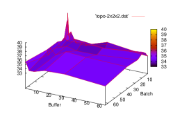
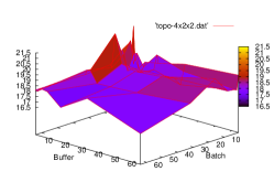
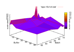
Figure 1: Time to check for mutual exclusion for 20 trains qualitatively.

We see, modulo experimental variations, that the algorithm improves when the batches or buffer are increased but then it becomes quickly insensitive to these parameters.

Distributing the estimation algorithm is much simpler. We need a fixed number of runs determined by the Chernoff’s bound [12] to conclude on a probability value with given confidence level. This is an embarrassingly parallel problem since we can simply divide the work equally and gather the result at the end. To compensate for fluctuations in the cluster, we could implement work-stealing but as our experiments show, this does not seem to be necessary since the observed performance scales almost linearly. The loss in efficiency in the later cases exhibits the overhead of starting up all the processors (around 3-4 seconds), which would be compensated for much longer runs. Figure 1 shows running time and relative efficiency for checking a few quantitative properties on the Firewire and LMAC protocol.

	Firewire					LMAC
PxC/N	1	2	4	8	16	1	2	4	8	16
1x1	621.7s	316.7s	160.2s	81.1s	44.7s	279.3s	140.7s	73.0s	37.0s	19.5s
	1.00	0.98	0.97	0.96	0.87	1.00	0.99	0.96	0.94	0.90
1x2	300.9s	162.2s	80.5s	47.6s	24.3s	144.3s	71.0	37.5s	19.2s	10.4s
	1.03	0.96	0.97	0.82	0.80	0.97	0.98	0.93	0.91	0.84
1x4	161.2s	84.0s	44.8s	24.1s	16.0s	74.2s	36.1s	19.3s	9.6s	8.1s
	0.96	0.93	0.87	0.81	0.61	0.94	0.97	0.90	0.91	0.54
2x4	85.1s	46.5s	23.1s	14.1s	8.5	35.5s	19.6s	10.1s	10.2s	6.4s
	0.91	0.84	0.84	0.69	0.57	0.98	0.89	0.86	0.43	0.34

Table 1: Time in seconds and efficiency (italic) to checking quantitative properties on the Firewire and LMAC model in function of the number of nodes (N), processors per node (P) and cores per processor (C).

4 Distributed Parametric Model-Checking: The Principle

In many practical cases system behaviors depend on the values of a finite set of constant parameters. For instance, these parameters can define network topology, or transmission rate of a node.

An interesting question might be to study how a system behavior depends on the values of these parameters. This may include visualisation of this dependency (drawing plots), optimization/worst case analysis and determining the correlation between different parameters. Another example that we will study below is computing Nash Equilibrium in wireless ad-hoc networks, e.g. choosing a network configuration that is stable with respect to the behavior of selfish nodes.

Let us assume that there is a finite set of parameters, each defined on a finite domain. We will model parameterized systems using Uppaal models in which some integer constants (transition weights or constants in variable assignment/clock invariants) are parameterized, e.g. they are replaced by special syntactic constructs that define the sets of possible values. Currently, we support two constructs:

• #range(a, b) defines the set of all integers between a and b,

• #booleanmatrix(N) defines the set of all boolean matrices of size N, this construct can be used to represent the set of all possible topologies of a network with N nodes.

We developed a framework for solving the “parametric” problems listed above (visualisation, optimization/worst case analysis, Nash Equilibrium computation). In order to solve all these problems our implementation performs a series of invocations of Uppaal-smc for different values of parameters. These invocations are independent of each other, thus they can be easily distributed on highly heterogeneous clusters. Our implementation uses the SLURM batch system [20], or it can submit jobs to the computational nodes using SSH connection by its own.

5 Distributed Parametric Model Checking: Case-Studies

5.1 Traingate example

We consider a model of a railway bridge [19] where several trains are crossing a bridge with one track. Our Uppaal model is depicted on Fig. 2. Trains start in the Safe initial location where they are not approaching. They will leave that location and be approaching (and go to location Appr) with an arrival rate given by the expression 1:#range(1,20) on the figure. This is a parameter declaration that will be used to generate models with values 1:1, 1:2, …1:20. This expression (of the form $i:j$) is an extension of Uppaal and defines an exponential distribution with the rate $\frac{i}{j}$ to pick the delay from. When a train is approaching, it enters Appr and synchronizes with appr[id]!. The gate controller will know that train id is approaching. After 10 time units the train will be crossing (enter location Cross, unless it is stopped before by the gate controller. This is done with the synchronization stop[id]? and the train goes to the location Stop. From there, it is restarted with the synchronization go[id]? by the gate controller and after 7 time units it will be crossing. After crossing, trains leave the bridge with leave[id]! and are safe again and can decide to approach again.

The gate controller keeps track of stopped trains with a FIFO queue (not depicted here) that we will not detail. Trains are queued and dequeued with this queue with the help of functions as seen on the figure. The gate has two main states Free and Occ (i.e. occupied) that keeps track of the state of the bridge. If trains are approaching then it either stops them if the bridge is occupied or let them pass otherwise. When the bridge becomes free (one train leaves), the controller decides to restart a train at the front of the queue with go[front()]!.

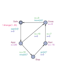
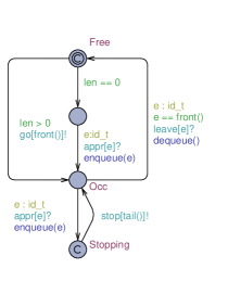
Figure 2: Uppaal models of a train (left) and a gate controller (right).

Here a (qualitative) safety means to ensure that at most one train can be in the crossing at the same time, and such property can be checked using classical Uppaal model checker. On top of that, now Uppaal-smc can also evaluate probabilistic (quantitative) properties. For instance, we can estimate the probability that the first train will cross the bridge within $50$ time units by checking a PWCTL property $\Diamond_{time\leq 50}\big{(}Train(0).Cross\big{)}$.

Consider two parameters in our model: the number of trains, and the rate with which these trains are coming. The rate parameter is on location ‘Safe shown in Fig. 2, and the number of trains is declared similarly in the System declarations.

Fig. 3 depicts the results of a parameter sweep of this model. The plot shows that when the number of trains increases, the probability that the first train will cross the bridge within $50$ time units decreases. Indeed, it is more likely that it will be stopped by other trains (there are more) and spend time in the Stop location. When the arrival rate is decreased, the probability also decreases.

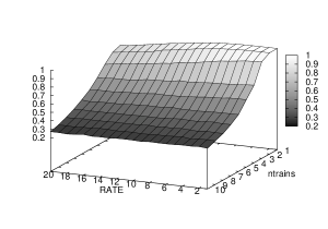
Figure 3: Parametric sweep for the traingate model.

5.2 Nash equilibrium Aloha CSMA/CD protocol

Aloha protocol [2] is a simple Carrier Sense Multiple Access with Collision Detection (CSMA/CD) protocol that was used in the first known wireless data network developed at the University of Hawaii in 1971. The protocol assumes that there are several nodes that share the same wireless medium. Each node is listening to its own signal during its transmission and checks that the signal is not corrupted by a simultaneous transmission by another node. In case of collision both nodes stop transmitting immediately and wait for a random time before they try to transmit again.

The Uppaal model of a single node is given in Fig. 4. We consider unslotted Aloha where the nodes are not necessary synchronized. Additionally, we study the p-persistent variant of Aloha, i.e. a protocol implementation in which a random delay before retransmission is distributed according to a geometric distribution. This means that in each time slot a node transmits with probability TransmitProb and waits for one more slot (and then decide again) with probability $1-$TransmitProb.

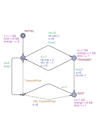
Figure 4: Model of Aloha in Uppaal

In our experiments we assumed that the goal of a node is to transmit a single frame within $50$ time units and to limit energy consumption by $3$. This goal for a node $i$ can be expressed using the following PWCTL formula:

$$\psi_{i}\equiv\Diamond_{Node(i).time\leq 50}(Node(i).ns\geq 1\wedge Node(i).energy\leq 3)$$ (1)

Then the utility function $U_{i}$ of a node $i$ is equal to the probability that the goal $\psi_{i}$ is satisfied by a random run of a system, i.e:

$$U_{i}(p_{1},p_{2},\dots,p_{N})\equiv Pr[S(p_{1},p_{2},\dots,p_{N})\models\psi_{i}]$$ (2)

, where $p_{j}$ is equal to the value of TransmitProb chosen by node $j$.

We consider the case where there is a master node that knows the network configuration (here the number of nodes) and broadcasts the value of TransmitProb parameter to all the nodes. Now, if there are selfish nodes, they can change their values of TransmitProb to achieve better performance (and other nodes will suffer from that). Thus, the interesting question is to find the value of TransmitProb that satisfies Nash Equilibrium (NE). For such a value, it is not profitable for any node to alter its behaviour to the detriment of other nodes. For our case the network is symmetric, thus we can search for $NE$ from the point of view of the first node only. In other words, parameter $p$ satisfies NE, iff $U_{0}(p,p,\dots,p)$ is larger than $U_{0}(p^{\prime},p,\dots,p)$ for any $p^{\prime}$.

Table 2: Nash equilibrium (NE) and Symmetric optimal (Opt) strategies for Aloha.

Number of nodes	2	3	4	5	6	7
NE strategy $p_{NE}$	0.37	0.40	0.35	0.35	0.41	0.42
$\widetilde{U}(p_{NE},p_{NE})$	0.99	0.98	0.95	0.89	0.75	0.61
Symmetric optimal strategy $p_{opt}$	0.30	0.30	0.26	0.22	0.19	0.15
$\widetilde{U}(p_{Opt},p_{opt})$	0.99	0.98	0.96	0.90	0.87	0.98
Computation time	2m5s	3m44s	7m62s	15m45s	26m11s	37m55s

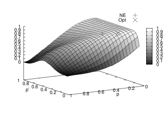
Figure 5: Utility function (left) and its diagonal slice (right) for Aloha with $5$ nodes.

Fig. 5 depicts the plot of the utility function $U_{0}(p^{\prime},p,\dots,p)$ for the network of $5$ nodes for different values of $p^{\prime}$ and $p$. Here $p^{\prime}$ is a value of TransmitProb of a potentially selfish node, and $p$ is a value for other nodes. You can also see the computed values of Nash Equlibrium (NE) parameter and symmetric optimal (Opt) parameter.

Table 2 contains the found values of Nash Equilibrium for Aloha with different number of nodes. The experiments were done on a 8-node cluster, where each node uses Intel(R) Core(TM)2 Quad CPU 2.66GHz processor.

5.3 Parameterized Topology for Network Models

There are situations The performance of some network protocols can depend not only on retransmission parameters as seen previously but also on the actual topology of the network. In this section we study the impact of different topologies on the LMAC protocol.

LMAC is a Lightweight Media Access protocol (studied in [8, 10]) used for scheduling communication in wireless sensor networks where the topology is determined by physical location and radio connectivity of the individual nodes. One of the goals of the LMAC protocol is to minimize the number of collisions in the network and to reconfigure the network to avoid further collisions. The difficulty of studying such protocols stems from the fact that the topology is not known in advance and there are exponentially many topologies (at least $n\cdot 2^{n-1}$ for $n$ nodes with one of them being a gateway), which makes systematic analysis of large networks impractical. In order to study the robustness of the LMAC protocol against collisions, we propose to examine hundreds of random topologies and then pick and focus on the most problematic ones. Listing 1 shows how a topology is declared in the Uppaal model: a two-dimensional array of boolean constants gives the adjacency matrix of the network graph. The receivers then use the guard can_hear[receiver][sender] when listening for the broadcast channel synchronizations.

⬇

1const int NODES = 10; // number of nodes

2typedef int[0,NODES$-$1] nodeid_t; // used to identify node

3typedef bool topology_t[nodeid_t][nodeid_t]; // type for topology

4const topology_t can_hear = #binarymatrix(NODES, NODES); // adjacency matrix

Listing 1: Network topology declaration in Uppaal model of LMAC.

In this case we try networks of up to ten nodes and twice as many slots, whereas one slot per node is enough to schedule flawless communication if only nodes were perfectly aware of each others choices. We used a property $Pr[\Diamond_{time\leq 2000}(col\_count>42)]$ estimating the probability of having more than 42 collisions after 2000 time units, which hints that there are perpetually reoccurring collisions.

The prepared model is then processed by our parametric model-checker that instantiates the keyword #binarymatrix with a concrete random matrix and distributes the verification on a cluster of computers, one instance of the matrix per core. Each verification uses Uppaal-smc. Using the naive randomization, a cluster of 32 cores (the same as in Section 5.2) can verify 10000 topologies in 6h 50min. Figure 6 shows the five topologies that yield the highest probabilities. We used low confidence (95%) statistical parameters to gain performance, thus the estimated probabilities have large $\pm 0.05$ statistical error, but the found topologies can be studied further in Uppaal-smc.

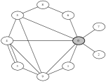
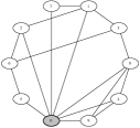
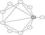
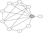
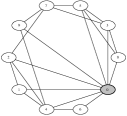
$p_{1}=0.630$	$p_{2}=0.629$	$p_{3}=0.617$	$p_{4}=0.607$	$p_{5}=0.599$

Figure 6: Highest probabilities found by model checking random topologies of 10 nodes.

Alternatively we tried generating all graphs up to 10 nodes which are unlikely to be isomorphic. The procedure is not guaranteed to cover all non-isomorphic classes (it may miss some), but it is very simple and can be recursively described as follows:

1. Start with a topology consisting of just one node.

2. Add a new node and consider two new topologies:

   1. Connect the new node to all the old nodes, go to step 2 until enough nodes are added.

   2. Leave the new node unconnected at all, go to step 2 until enough nodes are added.

3. For every node in a topology, make a new topology by marking the node as a gateway.

4. Get rid of the topologies where the gateway is not connected.

Up to the step 2 the procedure generates $2^{n-1}$ topologies which are non-isomorphic for sure, then steps 4 and 5 contain basic heuristics how to pick a gateway, which may yield some isomorphic graphs due to symmetric gateways, but the overhead is small.

Figure 7 shows the 5 cases that achieve the highest probability found by generating 5120 topologies of up to 10 nodes using our heuristics. The verification took about 3h 30min. The heuristic procedure has clear advantages over the randomized one but it is not exhaustive. On the other hand, the randomized method has the potential to find any topology but without any guarantee.

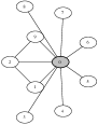
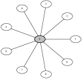
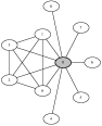
$p_{1}=0.919$	$p_{2}=0.905$	$p_{3}=0.898$	$p_{4}=0.894$	$p_{5}=0.888$

Figure 7: Highest probabilities found by model checking generated topologies of 10 nodes.

6 Conclusion

This paper proposes new algorithms to distribute statistical model checking algorithms through a master/slaves architecture. Our results have been implemented in the UPPAAL SMC toolset. A series of experiments show that our approach scales better than existing solutions [22].

As a future work, we will extend our distributed algorithms to the setting of rare events and unbounded temporal properties. We shall also implement and distribute Bayesian extensions of the approach we proposed in [14].

References

- [1]
- [2] Norman Abramson (1970): THE ALOHA SYSTEM: another alternative for computer communications. In: Proceedings of the November 17-19, 1970, fall joint computer conference, AFIPS ’70 (Fall), ACM, New York, NY, USA, pp. 281–285, 10.1145/1478462.1478502.
- [3] A. Basu, S. Bensalem, M. Bozga, B. Caillaud, B. Delahaye & A. Legay (2010): Statistical Abstraction and Model-Checking of Large Heterogeneous Systems. In: FORTE, LNCS 6117, Springer, pp. 32–46, 10.1007/978-3-642-13464-7_4.
- [4] M. Broy, B. Jonsson, J-P. Katoen, M. Leucker & A. Pretschner, editors (2005): Model-Based Testing of Reactive Systems, Advanced Lectures The volume is the outcome of a research seminar that was held in Schloss Dagstuhl in January 2004. Lecture Notes in Computer Science 3472, Springer, 10.1007/b137241.
- [5] J. R. Burch, E. M. Clarke, K. L. McMillan, D. L. Dill & L. J. Hwang (1992): Symbolic model checking: 1020 States and beyond. Information and Computation 98(2), pp. 142–170, 10.1016/0890-5401(92)90017-A.
- [6] E. M. Clarke, A. Donzé & A. Legay (2008): Statistical Model Checking of Mixed-Analog Circuits with an Application to a Third Order Delta-Sigma Modulator. In: Proc. of 3rd Haifa Verification Conference (HVC), LNCS 5394, Springer, pp. 149–163, 10.1007/978-3-642-01702-5_16.
- [7] Edmund M. Clarke, James R. Faeder, Christopher James Langmead, Leonard A. Harris, Sumit Kumar Jha & Axel Legay (2008): Statistical Model Checking in BioLab: Applications to the Automated Analysis of T-Cell Receptor Signaling Pathway. In Monika Heiner & Adelinde Uhrmacher, editors: Proceedings of the 6th International Conference on Computational Methods in Systems Biology (CMSB), LNCS, Springer, pp. 231–250, 10.1007/978-3-540-88562-7_18.
- [8] Alexandre David, Kim G. Larsen, Axel Legay, Marius Mikučionis, Danny Bøgsted Poulsen, Jonas Van Vliet & Zheng Wang (2011): Statistical Model Checking for Networks of Priced Timed Automata. In Uli Fahrenberg & Stavros Tripakis, editors: 9th International Conference on Formal Modeling and Analysis of Timed Systems (FORMATS), LNCS 6919, Springer, Aalborg, Denmark, pp. 80–96, 10.1007/978-3-642-24310-3.
- [9] Alexandre David, Kim G. Larsen, Axel Legay, Marius Mikučionis & Zheng Wang (2011): Time for Statistical Model Checking of real-time systems. In Ganesh Gopalakrishnan & Shaz Qadeer, editors: 23rd International Conference on Computer Aided Verification (CAV), LNCS 6806, Springer, Snowbird, UT, USA, pp. 349–355, 10.1007/978-3-642-22110-1.
- [10] Ansgar Fehnker, Lodewijk van Hoesel & Angelika Mader (2007): Modelling and Verification of the LMAC Protocol for Wireless Sensor Networks. In Jim Davies & Jeremy Gibbons, editors: Integrated Formal Methods, LNCS 4591, Springer Berlin / Heidelberg, pp. 253–272, 10.1007/978-3-540-73210-5_14.
- [11] R. Grosu & S. A. Smolka (2005): Monte Carlo Model Checking. In: Proc. of 11th Int. Conference on Tools and Algorithms for the Construction and Analysis of Systems (TACAS), LNCS 3440, Springer, pp. 271–286, 10.1007/978-3-540-31980-1_18.
- [12] Thomas Hérault, Richard Lassaigne, Frédéric Magniette & Sylvain Peyronnet (2004): Approximate Probabilistic Model Checking. In Bernhard Steffen & Giorgio Levi, editors: Verification, Model Checking, and Abstract Interpretation, LNCS 2937, Springer, pp. 307–329, 10.1007/978-3-540-24622-0_8.
- [13] D. N. Jansen, J-P Katoen, M.Oldenkamp, M. Stoelinga & I. S. Zapreev (2007): How Fast and Fat Is Your Probabilistic Model Checker? An Experimental Performance Comparison. In: HVC, LNCS 4899, Springer, 10.1007/978-3-540-77966-7_9.
- [14] Sumit Kumar Jha, Edmund M. Clarke, Christopher James Langmead, Axel Legay, André Platzer & Paolo Zuliani (2009): A Bayesian Approach to Model Checking Biological Systems. In: CMSB, LNCS 5688, Springer, pp. 218–234, 10.1007/978-3-642-03845-7_15.
- [15] Kenneth L. McMillan (1993): Symbolic Model Checking. Ph.D. thesis, Carnegie Mellon University.
- [16] Koushik Sen, Mahesh Viswanathan & Gul Agha (2004): Statistical Model Checking of Black-Box Probabilistic Systems. In: CAV, LNCS 3114, Springer, pp. 202–215, 10.1007/978-3-540-27813-9_16.
- [17] The UPPAAL Tool. Available at http://www.uppaal.com/.
- [18] Abraham Wald (2004): Sequential Analysis. Courier Dover Publications.
- [19] Wang Yi, Paul Pettersson & Mats Daniels (1994): Automatic Verification of Real-Time Communicating Systems by Constraint-Solving. In Dieter Hogrefe & Stefan Leue, editors: Proceedings of the 7th International Conference on Formal Description Techniques, North–Holland, London, UK, pp. 223–238. Available at http://dl.acm.org/citation.cfm?id=646213.681364.
- [20] Andy B. Yoo, Morris A. Jette & Mark Grondona (2003): SLURM: Simple Linux Utility for Resource Management. In Dror G. Feitelson, Larry Rudolph & Uwe Schwiegelshohn, editors: Job Scheduling Strategies for Parallel Processing, 9th International Workshop, JSSPP 2003, Seattle, WA, USA, June 24, 2003, Revised Papers, LNCS 2862, Springer, pp. 44–60, 10.1007/10968987_3.
- [21] Håkan L. S. Younes (2005): Verification and Planning for Stochastic Processes with Asynchronous Events. Ph.D. thesis, Carnegie Mellon University.
- [22] Håkan L. S. Younes (2005): Ymer: A Statistical Model Checker. In: Proc. of 11th Int. Conference on Computer Aided Verification (CAV), LNCS 3576, Springer, pp. 429–433, 10.1007/11513988_43.
- [23] Håkan L. S. Younes, Marta Z. Kwiatkowska, Gethin Norman & David Parker (2006): Numerical vs. statistical probabilistic model checking. International Journal on Software Tools for Technology Transfer (STTT) 8(3), pp. 216–228, 10.1007/s10009-005-0187-8.