Imbalanced ultracold Fermi gas in the weakly repulsive regime: Renormalization group approach for $p$-wave superfluidity

Abstract

We theoretically study a possible new pairing mechanism for a two-dimensional population imbalanced Fermi gas with short-range repulsive interactions which can be realized on the upper branch of a Feshbach resonance. We use a well-controlled renormalization group approach, which allows an unbiased study of the instabilities of imbalanced Fermi liquid without assumption of a broken symmetry and gives a numerical calculation of the transition temperature from microscopic parameters. Our results show a leading superfluid instability in the $p$-wave channel for the majority species. The corresponding mechanism is that there are effective attractive interactions for the majority species, induced by the particle-hole susceptibility of the minority species, where the mismatch of the Fermi surfaces of the two species plays an important role. We also propose an experimental protocol for detecting the $p$-wave superfluidity and discuss the corresponding experimental signatures.

I Introduction

Much of the interest in ultracold atomic gases comes from their amazing tunability. Experiments on ultracold atomic gases allow fermionic pairing phenomena to be manipulated much more precisely and controllably than those in solid state systems. There are many important experiments in ultracold gases which undoubtedly illustrate this advantage, such as the crossover from Bose-Einstein condensation (BEC) to Bardeen-Cooper-Schrieffer (BCS) superfluidity with the help of Feshbach resonance Regal et al. (2004); Zwierlein et al. (2004); Chin et al. (2004); Kinast et al. (2004), and superfluid-Mott insulator transitions with optical lattices Greiner et al. (2002); Stöferle et al. (2004).

Due to the wide-range tunability of the effective interatomic scattering length there are strong motivations to study the pairing phenomena with population imbalanced ultracold Fermi gases in different regimes. However, in ultracold Fermi gases, in contrast with solid state systems, the pairing state is not easily achieved due to the smallness of the gap parameter. Therefore, previous investigations on superfluidity of imbalanced Fermi gases mostly focused on the unitary regime where the scattering length is large Giorgini and Stringari (2008); Zwierlein et al. (2006); Gubbels and Stoof (2008); Patton and Sheehy (2011). In systems with attractive interactions, the presence of population imbalance can enrich the possibilities for pairing states. As predicted by previous works, there may be Larkin-Ovchinnikov-Fulde-Ferrell (LOFF) state Fulde and Ferrell (1964); Larkin and Ovchinnikov (1965); James and Lamacraft (2010), breached pair state Liu and Wilczek (2003); Gubankova et al. (2003); Forbes et al. (2005) and deformed Fermi surfaces Müther and Sedrakian (2002). Pairing can also occur when there are intermediate bosons for providing effective attractive interactions such as bosonic molecules in deep BEC regime, where there may be $p$-wave superfluidity Bulgac et al. (2006); Bulgac and Yoon (2009); Iskin and Sá de Melo (2007), and phonons of a dipolar condensate Kain and Ling (2011). Besides, in a system where the bare interactions are purely repulsive, there are also possibilities for effective attractive interactions to emerge. It was first studied by Kohn and Luttinger Kohn and Luttinger (1965), where a three-dimensional (3D) electron system was considered. In 3D electron systems, the particle-hole susceptibility $\chi(k)$ has a strong $k$ dependence for $k\leqslant 2k_{F}$, which is responsible for the emergence of effective attractive interactions in high angular-momentum channel. However, dimensionality can significantly change the behavior of $\chi(k)$. In two dimension (2D), $\chi(k)$ is momentum independent when $k\leqslant 2k_{F}$, and there may be superfluid instability in the presence of population imbalance Raghu and Kivelson (2011), which is different from the Kohn-Luttinger type.

In this paper, we consider a population imbalanced 2D ultracold Fermi gases in the weakly repulsive regime, which can be realized on the upper branch of a Feshbach resonance Jo et al. (2009). There are two novelties in our system that should be emphasized. Firstly, the bare interactions between atoms of two different hyperfine states are purely repulsive. Secondly, there are no intermediate bosons for providing effective attractive interactions such as phonons in traditional superconductors or bosonic molecules at the BEC side of a Feshbach resonance. Our study shows that there is an alternative choice of $p$-wave superfluid state induced by the population imbalance, which fundamentally breaks the spin rotation symmetry. The particle-hole susceptibility of the minority species can induce an attractive interaction for the majority species because of the population imbalance. This mechanism of superfluidity resembles qualitatively the situation in the $A_{1}$ phase of superfluid ${}^{3}\mathrm{He}$ Vollhardt and Wölfle (1990) and 2D electronic gases Raghu et al. (2010); Raghu and Kivelson (2011).

Our theoretical framework is heavily based on the renormalization group (RG) theory for interacting fermion systems Shankar (1991, 1994); Polchinski (1994); Weinberg (1994). The RG framework provides us a powerful tool to treat competing instabilities simultaneously, and most importantly, to justify the leading instability channel Shankar (1994). Furthermore, we can identify the critical temperature from the onset of the instability channel Tsai et al. (2005). By performing RG process at finite temperature and solving the flow equations numerically, we can obtain the phase transition between normal state and $p$-wave superfluid state. Within this framework, in the second stage of RG, when mode eliminations have reached an momentum cutoff $\Lambda$ far smaller than the Fermi momentum $K_{F}$, a large-N expansion emerges with $N=K_{F}/\Lambda$, which is a strong suggestion for us to extend our results from weak to intermediate coupling regime Shankar (1994).

The paper is organized as follows: The first stage of the RG approach for building the model of interacting imbalanced fermions is described in Sec. II. Sec. III illustrates the non-perturbative RG method for unequal Fermi surfaces and obtain the flow equations. The RG analysis indicates a leading instability in the $p$-wave Cooper channel when the population imbalance is present. In Sec. IV we numerically solve the flow equation at finite temperature. We obtain the critical temperature at which the normal Fermi liquid state becomes unstable in the $p$-wave Cooper channel. Furthermore, with the large-$N$ analysis, we extend our results from weak coupling regime to intermediate coupling regime where we may have higher critical temperature. Sec. V contains experimental discussions and conclusions.

II Model building: The first stage of RG

We consider a population imbalanced Fermi gas with short-range Hubbard repulsive interactions, whose partition function

$$\mathcal{Z}=\int\,D[\bar{\psi},\psi]e^{-S[\bar{\psi},\psi]}$$ (1)

with

$$S[\bar{\psi},\psi]=S_{0}[\bar{\psi},\psi]+S_{I}[\bar{\psi},\psi],$$ (2)

where $S_{0}$ is the free part,

$$S_{0}[\bar{\psi},\psi]=\sum_{k,\sigma}\bar{\psi}_{\sigma}(k)(-ik_{n}-\mu_{\sigma}+E(\boldsymbol{k}))\psi_{\sigma}(k).$$ (3)

$k$ is short for $(k_{n},\boldsymbol{k})$. $\sigma=\uparrow$ or $\downarrow$ represents two different hyperfine states. $E(\boldsymbol{k})=\boldsymbol{k}^{2}/(2m)$ is the free energy of atoms. $\mu_{\sigma}$ is the chemical potential, and the Fermi momentum satisfies $\mu_{\sigma}=K_{F\sigma}^{2}/(2m)$. Population imbalance is put in by setting $\mu_{\uparrow}\neq\mu_{\downarrow}$ ( Without loss of generality, we can assume $\mu_{\uparrow}>\mu_{\downarrow}$. ). We work at finite temperature, with imaginary time formulism, where $k_{n}$ is the fermionic Matsubara frequency. The interacting part of the action reads

$$S_{I}[\bar{\psi},\psi] = \frac{U}{\beta V}\sum_{\{k_{i}\}}\bar{\psi}_{\uparrow}(k_{1})\bar{\psi}_{\downarrow}(k_{2})\psi_{\downarrow}(k_{3})\psi_{\uparrow}(k_{4})$$ (4)

$$\times\delta_{k_{1n}+k_{2n},k_{3n}+k_{4n}}\delta(\boldsymbol{k}_{1}+\boldsymbol{k}_{2}-\boldsymbol{k}_{3}-\boldsymbol{k}_{4}).$$

The basic idea of RG is to gradually integrate out “faster” degrees of freedom which have larger momentums locating in a shell region in momentum space and see how the resulting effective Hamiltonian will flow under such process. To begin the RG process, we first introduce an artificial energy scale $\Omega_{0}$ and integrate out degrees of freedom with energies higher than $\Omega_{0}$ to obtain the effective theory of the system at energy scale $\Omega_{0}$. We assume that the bare Hamiltonian is in the weak coupling regime. Thus, if we choose $\Omega_{0}$ not much lower than the ultraviolet cutoff of the bare Hamiltonian, the “integrating out” procedure can be done by using straightforward perturbative approach because there is no significant renormalization of the coupling parameters.

In detail, we first divide the degrees of freedom of the system into “slow modes”

$$\psi_{\sigma}^{<}=\psi_{\sigma}(k),\bar{\psi}_{\sigma}^{<}=\bar{\psi}_{\sigma}(k)\;\text{for}\;|\varepsilon_{\boldsymbol{k},\sigma}|<\Omega_{0}$$ (5)

and “fast modes”

$$\psi_{\sigma}^{>}=\psi_{\sigma}(k),\bar{\psi}_{\sigma}^{>}=\bar{\psi}_{\sigma}(k)\;\text{for}\;|\varepsilon_{\boldsymbol{k},\sigma}|>\Omega_{0},$$ (6)

where $\varepsilon_{\boldsymbol{k},\sigma}=E(\boldsymbol{k})-\mu_{\sigma}$.

We then carry out the “modes elimination” by integrating out the fast modes and this can be formally written as

$$Z = \int D[\bar{\psi},\psi]\mathrm{e}^{-S[\bar{\psi},\psi]}$$ (7)

$$= \int D[\bar{\psi}^{<},\psi^{<},\bar{\psi}^{>},\psi^{>}]$$

$$\times\;\mathrm{e}^{-S[\bar{\psi}^{<},\psi^{<}]-S[\bar{\psi}^{>},\psi^{>}]-S_{2}[\bar{\psi}^{<},\psi^{<},\bar{\psi}^{>},\psi^{>}]}$$

$$= \int D[\bar{\psi}^{<},\psi^{<}]\mathrm{e}^{-S[\bar{\psi}^{<},\psi^{<}]}$$

$$\times\;\int D[\bar{\psi}^{>},\psi^{>}]\mathrm{e}^{-S[\bar{\psi}^{>},\psi^{>}]-S_{2}[\bar{\psi}^{<},\psi^{<},\bar{\psi}^{>},\psi^{>}]}$$

$$\equiv \int D[\bar{\psi}^{<},\psi^{<}]\mathrm{e}^{-S^{\Omega_{0}}[\bar{\psi}^{<},\psi^{<}]}.$$

After gathering all terms independent of $\bar{\psi}^{>}$ and $\psi^{>}$ into $S[\bar{\psi}^{<},\psi^{<}]$ , the rest terms can be written as $-S[\bar{\psi}^{>},\psi^{>}]-S_{2}[\bar{\psi}^{<},\psi^{<},\bar{\psi}^{>},\psi^{>}]$, and $S^{\Omega_{0}}$ is the resulting effective action at energy scale $\Omega_{0}$.

Generally, $S^{\Omega_{0}}$ has the form:

$$S^{\Omega_{0}}[\bar{\psi},\psi]=S_{0}^{\Omega_{0}}[\bar{\psi},\psi]+S_{I}^{\Omega_{0}}[\bar{\psi},\psi],$$ (8)

where $S_{0}^{\Omega_{0}}[\bar{\psi},\psi]$ is the free action,

$$S_{0}^{\Omega_{0}}[\bar{\psi},\psi]=\sum_{k}^{\Omega_{0}}\,\bar{\psi}(k)(-ik_{n}-\mu+\tilde{E}(\boldsymbol{k}))\psi(k)$$ (9)

and $S_{I}^{\Omega_{0}}[\bar{\psi},\psi]$ is the interacting action which will have the most generic form after the “integrating out” procedure.

$$S_{I}^{\Omega_{0}}[\bar{\psi},\psi] = \frac{1}{\beta V}\sum_{\{k_{i},\sigma_{i}\}}^{\Omega_{0}}u(k_{1},\sigma_{1},k_{2},\sigma_{2},k_{3},\sigma_{3},k_{4},\sigma_{4})$$ (10)

$$\times\bar{\psi}_{\sigma_{1}}(k_{1})\bar{\psi}_{\sigma_{2}}(k_{2})\psi_{\sigma_{3}}(k_{3})\psi_{\sigma_{4}}(k_{4})$$

$$\times\delta_{k_{1n}+k_{2n},k_{3n}+k_{4n}}\delta_{\sigma_{1}+\sigma_{2}-\sigma_{3}-\sigma_{4},0}$$

$$\times\delta(\boldsymbol{k}_{1}+\boldsymbol{k}_{2}-\boldsymbol{k}_{3}-\boldsymbol{k}_{4}).$$

where the superscript $\Omega_{0}$ of the summation operator means the summation is done within the slow modes characterized by the energy scale $\Omega_{0}$ (Eq. (5)).

With singlet pairing suppressed by imbalance, we shall consider triplet pairing between fermions with the same spin. As shown in Fig. 1, the induced interaction within the same spin species in the Cooper channel is of order $U^{2}$ and depends on external momentums and frequencies. However, only the constant term of a coupling function is not irrelevant in the tree level scaling Shankar (1994). Therefore, we will focus on the induced Cooper channel effective interaction of order $U^{2}$ with external momentums set on the Fermi surface and external frequencies set to zero. In this case, the interaction vertex will only depend on the orientations of the incoming and outgoing momentums and can be written as

$$\Gamma_{\sigma}(\hat{\boldsymbol{k}},\hat{\boldsymbol{k}}^{\prime})=U^{2}\chi_{-\sigma}(\boldsymbol{k}-\boldsymbol{k}^{\prime}).$$ (11)

$\chi_{\sigma}(\boldsymbol{k})$ is the susceptibility at zero frequency:

$$\chi_{\sigma}(\boldsymbol{k}) = \int_{p}G_{\sigma}(ip_{n},\boldsymbol{p})G_{\sigma}(ip_{n},\boldsymbol{p+k})$$ (12)

$$= \int\frac{\mathrm{d}^{2}p}{(2\pi)^{2}}\frac{f(\varepsilon_{\boldsymbol{p+k},\sigma})-f(\varepsilon_{\boldsymbol{p},\sigma})}{\varepsilon_{\boldsymbol{p+k},\sigma}-\varepsilon_{\boldsymbol{p},\sigma}},$$

where $f$ is the Fermi-Dirac distribution function, and $\int_{p}\equiv\frac{1}{\beta}\sum_{p_{n}}\int\frac{\mathrm{d}^{2}p}{(2\pi)^{2}}$. Because the susceptibility is not singular in the limit $\Omega_{0}\rightarrow 0$ ($\Omega_{0}\ll\mu$), we can only keep the zeroth order term by setting $\Omega_{0}=0$.

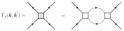
Figure 1: Interaction vertex within the same spin species at order $U^{2}$. It is induced by the susceptibility of “fast modes” with opposite spins. The propagators of fermions with spins opposite to the external ones are represented by dashed lines.

III The second stage of RG

After obtaining the effective action at energy scale $\Omega_{0}$ around the Fermi surface, Shankar’s RG Shankar (1994) for fermions can be carried out. We use the field-theory approach and calculate the four-point vertex at one-loop order at energy scale $\Omega$ (see Fig. 2 ):

$$\Gamma^{(4)}_{\sigma}(\hat{\boldsymbol{k}},\hat{\boldsymbol{k}^{\prime}}) = \Gamma_{\sigma}(\hat{\boldsymbol{k}},\hat{\boldsymbol{k}^{\prime}})$$ (13)

$$-\int_{p}^{\Omega}\frac{\Gamma_{\sigma}(\hat{\boldsymbol{k}},\hat{\boldsymbol{p}})\Gamma_{\sigma}(\hat{\boldsymbol{p}},\hat{\boldsymbol{k}^{\prime}})}{(ip_{n}-\varepsilon_{\boldsymbol{p},\sigma})(-ip_{n}-\varepsilon_{\boldsymbol{p},\sigma})},$$

where $\int_{p}^{\Omega}$ means the momentum integral is restricted in the shell region in momentum space with energy deviation less than $\Omega$ with respect to Fermi energy, and $\Omega$ is a energy scale within $\Omega_{0}$, i.e. $\Omega<\Omega_{0}$. The one-loop correction can be further carried out as:

$$-\frac{1}{\beta}\sum_{n}\int^{\Lambda_{\sigma}}\frac{p\mathrm{d}p}{2\pi}\int_{0}^{2\pi}\frac{\mathrm{d}\theta}{2\pi}\frac{\Gamma_{\sigma}(\hat{\boldsymbol{k}},\hat{\boldsymbol{p}})\Gamma_{\sigma}(\hat{\boldsymbol{p}},\hat{\boldsymbol{k}^{\prime}})}{(ip_{n}-\varepsilon_{\boldsymbol{p},\sigma})(-ip_{n}-\varepsilon_{\boldsymbol{p},\sigma})}$$ (14)

$$= -\!\int^{\Lambda_{\sigma}}\!\frac{p\mathrm{d}p}{2\pi}\int_{0}^{2\pi}\frac{\mathrm{d}\theta}{2\pi}\frac{\Gamma_{\sigma}(\hat{\boldsymbol{k}},\hat{\boldsymbol{p}})\Gamma_{\sigma}(\hat{\boldsymbol{p}},\hat{\boldsymbol{k}^{\prime}})}{2\varepsilon_{\boldsymbol{p}\sigma}}\tanh\frac{\beta\varepsilon_{\boldsymbol{p}\sigma}}{2}$$

where $\Lambda_{\sigma}$ is the momentum cutoff corresponding to $\Omega$, and $\int^{\Lambda_{\sigma}}$ is short for $\int_{|p-K_{F\sigma}|<\Lambda_{\sigma}}$. Due to $\Omega\ll\mu_{\uparrow(\downarrow)}$, we can approximate $\Omega$ as $v_{F\sigma}\Lambda_{\sigma}$, where $v_{F\sigma}$ is the Fermi velocity of atoms with spin $\sigma$.

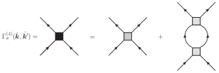
Figure 2: Four-point vertex for the effective action at energy scale $\Omega_{0}$ in the Cooper channel at one-loop order. Loop momentums are restricted in the thin shell around Fermi surface.

Because the four-point vertex is related to the scattering amplitude of certain scattering process, which is a physical observable, it should not depend on cutoff:

$$\frac{\mathrm{d}\Gamma^{(4)}_{\sigma}(\hat{\boldsymbol{k}},\hat{\boldsymbol{k}^{\prime}})}{\mathrm{d}l}=0,$$ (15)

where $l=\ln(\Omega_{0}/\Omega)=\ln(\Lambda_{0}/\Lambda)$.

From Eq. (15), we can get the flow equation as following

$$\frac{\mathrm{d}\Gamma_{\sigma}(\hat{\boldsymbol{k}},\hat{\boldsymbol{k}^{\prime}})}{\mathrm{d}l}=-\rho\!\int_{0}^{2\pi}\!\frac{\mathrm{d}\theta}{2\pi}\Gamma_{\sigma}(\hat{\boldsymbol{k}},\hat{\boldsymbol{p}})\Gamma_{\sigma}(\hat{\boldsymbol{p}},\hat{\boldsymbol{k}^{\prime}})\tanh\frac{\beta\Omega}{2}$$ (16)

where $\rho=m/2\pi$ is the 2D density of states. This is an ordinary differential equation for matrix $\Gamma_{\sigma}(\hat{\boldsymbol{k}},\hat{\boldsymbol{k}^{\prime}})$ with initial condition:

$$\Gamma_{\sigma}(\hat{\boldsymbol{k}},\hat{\boldsymbol{k}^{\prime}};\Omega_{0})=U^{2}\chi_{-\sigma}(\boldsymbol{k}-\boldsymbol{k}^{\prime}),$$ (17)

where $\Gamma_{\sigma}(\hat{\boldsymbol{k}},\hat{\boldsymbol{k}^{\prime}};\Omega_{0})$ denotes the effective interaction vertex at energy scale $\Omega_{0}$. For convenience, we define a dimensionless coupling function $g_{\sigma}(\hat{\boldsymbol{k}},\hat{\boldsymbol{k}^{\prime}};\Omega_{0})\equiv\rho\Gamma_{\sigma}(\hat{\boldsymbol{k}},\hat{\boldsymbol{k}^{\prime}};\Omega_{0})$. In the presence of rotational symmetry, $g_{\sigma}(\hat{\boldsymbol{k}},\hat{\boldsymbol{k}^{\prime}})$ only depends on the relative angle between the incoming and outgoing momentum, and the flow equation can be decomposed into uncoupled equations for eigenvalues of channels with different angular momentums Weinberg (1994):

$$\frac{\mathrm{d}\lambda_{\sigma m}}{\mathrm{d}l}=-(\lambda_{\sigma m})^{2}\tanh\frac{\beta\Omega}{2},$$ (18)

where $m$ labels different angular momentum channels.

The right hand side of Eq. (18) is negative definite, which means that for an initially attractive channel, $\lambda_{\sigma m}$ may be renormalized to negative infinity as the energy scale goes down to the Fermi energy. A qualitative argument of the critical temperature can be given based on Eq. (18). At low temperatures, $\tanh(\beta\Omega/2)$ equals almost unity for nearly all $\Omega$’s when $\Omega>0$, and drops rapidly to zero as $\Omega$ approaches zero from about $\Omega\sim k_{B}T$. Therefore, when temperature is low enough, we can approximate $\tanh(\beta\Omega/2)$ to be unity, and easily get the solution of Eq. (18), which guarantees a divergence at a certain energy scale. If this energy scale is higher than $k_{B}T$, the approximation used above is self-consistent, and the divergence indicates the superfluid instability. In other words, this energy scale gives a qualitative estimation of the critical temperature.

Results obtained by using the methods introduced above will certainly depend on the energy scale $\Omega_{0}$. However, it is clear that $\Omega_{0}$ is more a calculation device than a physical energy scale Raghu et al. (2010). Any physical predictions should not depend on $\Omega_{0}$. In fact, like RG in quantum field theory, we can make results independent of $\Omega_{0}$ at any order of $U$. This can be achieved by simply considering diagrams of the same order as the ones in the second stage when carrying out the perturbative calculations in the first stage Raghu et al. (2010); Efremov et al. (2000).

In detail, we have to take an additional term into account (see Fig. 3) and take $\tilde{\Gamma}_{\sigma}(\hat{\boldsymbol{k}},\hat{\boldsymbol{k}^{\prime}};\Omega_{0})$ as the initial condition for the second stage.

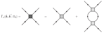
Figure 3: Induced interaction vertex at energy scale $\Omega_{0}$ after reconsidering a $U^{4}$ order correction, which is responsible for removing the $\Omega_{0}$ dependence. The loop modes are the “fast” ones, whose corresponding on-shell energies are larger than $\Omega_{0}$.

$$\tilde{\Gamma}_{\sigma}(\hat{\boldsymbol{k}},\hat{\boldsymbol{k}^{\prime}};\Omega_{0})$$ (19)

$$= \Gamma_{\sigma}(\hat{\boldsymbol{k}},\hat{\boldsymbol{k}^{\prime}})-\int^{>\Omega_{0}}_{p}\frac{\Gamma_{\sigma}(\hat{\boldsymbol{k}},p)\Gamma_{\sigma}(p,\hat{\boldsymbol{k}^{\prime}})}{(ip_{n}-\varepsilon_{\boldsymbol{p},\sigma})(-ip_{n}-\varepsilon_{\boldsymbol{p},\sigma})},$$

which has a similar form as Eq. (13) except that the region of the momentum integral is the area besides the thin shell around the Fermi surface and the dependence of the vertex on the magnitudes of momentums and frequencies should also be considered.

We first consider the frequency summation in the second term of Eq. (19). Most contribution comes from neighborhood of $p_{0}\sim 0$ and $|\boldsymbol{p}|\sim K_{F\sigma}$, so we can first set frequencies in $\Gamma^{\prime}s$ to zero. Then the frequency summation can be carried out as:

$$\tilde{\Gamma}_{\sigma}(\hat{\boldsymbol{k}},\hat{\boldsymbol{k}^{\prime}};\Omega_{0})$$ (20)

$$= \Gamma_{\sigma}(\hat{\boldsymbol{k}},\hat{\boldsymbol{k}^{\prime}})-\int_{\Lambda_{\sigma 0}}\frac{p\mathrm{d}p}{2\pi}\int_{0}^{2\pi}\frac{\mathrm{d}\theta}{2\pi}\frac{\Gamma_{\sigma}(\hat{\boldsymbol{k}},\boldsymbol{p})\Gamma_{\sigma}(\boldsymbol{p},\hat{\boldsymbol{k}^{\prime}})}{2\varepsilon_{\boldsymbol{p}\sigma}}$$

$$\times\tanh\frac{\beta\varepsilon_{\boldsymbol{p}\sigma}}{2},$$

where $\Lambda_{\sigma 0}=\Omega_{0}/v_{F\sigma}$.

Because the bare interaction is short-range and the Fermi gas is dilute which means the interatomic distance is much larger than the range of the interatomic interaction i.e. $K_{F\uparrow}^{-1}\gg r_{0}$, we can introduce an ultraviolet cutoff $\Lambda_{H}=2K_{F\uparrow}$ here. In the second term of Eq. (20) $\Gamma_{\uparrow}$ does not vary much with respect to momentum within this cutoff Raghu and Kivelson (2011) at low temperatures compared with the notable dependence of the other term on momentum. Therefore, we can neglect the dependence of the $\Gamma^{\prime}s$ on the magnitude of the momentums. Using the dimensionless coupling function which has been defined above as $g_{\sigma}(\hat{\boldsymbol{k}},\hat{\boldsymbol{k}^{\prime}};\Omega_{0})\equiv\rho\Gamma_{\sigma}(\hat{\boldsymbol{k}},\hat{\boldsymbol{k}^{\prime}};\Omega_{0})$ the initial condition of the flow equation can be written as

$$\tilde{g}_{\sigma}(\hat{\boldsymbol{k}},\hat{\boldsymbol{k}^{\prime}};\Omega_{0})$$ (21)

$$= g_{\sigma}(\hat{\boldsymbol{k}},\hat{\boldsymbol{k}^{\prime}})-\int_{0}^{2\pi}\frac{\mathrm{d}\theta}{2\pi}g_{\sigma}(\hat{\boldsymbol{k}},\hat{\boldsymbol{p}})g_{\sigma}(\hat{\boldsymbol{p}},\hat{\boldsymbol{k}^{\prime}})$$

$$\times\left(F_{\sigma}(\Omega_{H})-F_{\sigma}(\Omega_{0})\right),$$

where $F_{\sigma}(\Omega)$ is an auxiliary function defined as

$$F_{\sigma}(\Omega)=\frac{1}{\rho}\int_{|\varepsilon_{\boldsymbol{p}\sigma}|<\Omega}\frac{p\mathrm{d}p}{2\pi}\frac{1}{2\varepsilon_{\boldsymbol{p}\sigma}}\tanh\frac{\beta\varepsilon_{\boldsymbol{p}\sigma}}{2}$$ (22)

With the help of Eq. (22), flow equation can be expressed as:

$$\frac{\mathrm{d}g_{\sigma}(\hat{\boldsymbol{k}},\hat{\boldsymbol{k}^{\prime}})}{\mathrm{d}\Omega} = \int_{0}^{2\pi}\frac{\mathrm{d}\theta}{2\pi}g_{\sigma}(\hat{\boldsymbol{k}},\hat{\boldsymbol{p}})g_{\sigma}(\hat{\boldsymbol{p}},\hat{\boldsymbol{k}^{\prime}})\frac{\mathrm{d}F_{\sigma}(\Omega)}{\mathrm{d}\Omega}.$$ (23)

It can also be written in a more compact form, regarding $g_{\sigma}(\hat{\boldsymbol{k}},\hat{\boldsymbol{k}^{\prime}})$ as a matrix $(\mathbf{g}_{\sigma})_{\hat{\boldsymbol{k}},\hat{\boldsymbol{k}^{\prime}}}$ Weinberg (1994),

$$\frac{\mathrm{d}\mathbf{g}_{\sigma}}{\mathrm{d}\Omega}=\mathbf{g}_{\sigma}\cdot\mathbf{g}_{\sigma}\frac{\mathrm{d}F_{\sigma}(\Omega)}{\mathrm{d}\Omega}.$$ (24)

As we mentioned earlier, because of the rotational symmetry of the system, the coupling function can be decoupled in the angular momentum representation, and Eq. (24) becomes a series of flow equations of individual eigenvalues,

$$\frac{\mathrm{d}\lambda_{\sigma m}}{d\Omega}=(\lambda_{\sigma m})^{2}\frac{\mathrm{d}F_{\sigma}}{\mathrm{d}\Omega}$$ (25)

with innitial conditions,

$$\lambda_{\sigma m}(\Omega_{0})=\lambda_{\sigma m}-(\lambda_{\sigma m})^{2}\left(F_{\sigma}(\Omega_{H})-F_{\sigma}(\Omega_{0})\right),$$ (26)

which can be easily integrated and gives

$$\lambda_{\sigma m}(\Omega)^{-1} = \left(\lambda_{\sigma m}-(\lambda_{\sigma m})^{2}(F_{\sigma}(\Omega_{H})-F(\Omega_{0}))\right)^{-1}$$ (27)

$$-F(\Omega)+F(\Omega_{0}).$$

To order $U^{4}$, we have

$$\lambda_{\sigma m}(\Omega)=(\lambda_{\sigma m}^{-1}+F_{\sigma}(\Omega_{H})-F_{\sigma}(\Omega))^{-1},$$ (28)

which is independent of $\Omega_{0}$, and controls the flow behavior of the coupling strengths. At zero temperature, as mentioned above, a negative eigenvalue will flow to infinity at certain energy scale and cause superfluid instability. As temperature goes higher, the divergence will appear at lower energy scale. When temperature reaches a certain critical value, the divergence will not arise until we renormalize to the Fermi surface. Above this critical value, no divergence exists during the whole renormalization process down to the Fermi surface, which means that the Fermi liquid state is stable in the corresponding channel.

IV Numerical solutions of RG flow equations

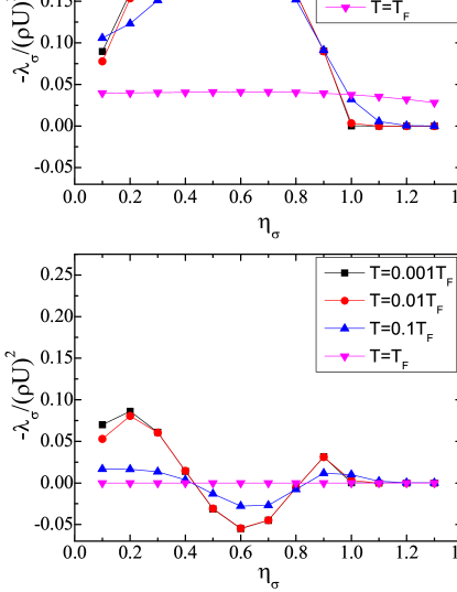
Figure 4: (Color online) Strength of the pairing interactions ( $-\lambda_{\sigma}/(\rho U)^{2}$) for spin spieces $\sigma$ in the $p$-wave (top) and $f$-wave (bottom) channels at different temperatures, where $\eta_{\sigma}$ is the imbalance ratio defined as $\eta_{\sigma}=K_{F-\sigma}/K_{F\sigma}$. The scales of the vertical axes of these two figures are chosen to be the same for convenient comparison.

In this section, we will determine the critical temperature by solving the flow equations numerically. As explained above, at critical temperature, we have

$$-\lambda_{\sigma m}^{-1}=F_{\sigma}(\Omega_{H})-F_{\sigma}(0).$$ (29)

For convenience, we can define some dimensionless parameters as follows $x_{\sigma}=k/K_{F\sigma},t_{\sigma}=T/T_{F\sigma}$, where $T_{F}$ is the Fermi temperature ($T_{F}^{\sigma}=\mu_{\sigma}/k_{B}$), and rewrite the susceptibility and the eigenvalues to the final form for numerical calculation.

Susceptibility only depends on the magnitude of momentum and can be written as

$$\chi_{\sigma}(x_{\sigma}) = \frac{1}{(2\pi)^{2}}\int_{0}^{\infty}p\mathrm{d}p\int_{0}^{2\pi}\mathrm{d}\theta f(\epsilon_{p,\sigma})\frac{2}{\epsilon_{p,\sigma}-\epsilon_{p+k,\sigma}}$$ (30)

$$= -\rho\int_{0}^{1}\mathrm{d}y\frac{y}{\sqrt{1-y^{2}}}\frac{1}{e^{((x_{\sigma}y/2)^{2}-1)/t_{\sigma}}+1}.$$

Eigenvalues of the dimensionless coupling function $g_{\sigma}$ have the form

$$\lambda_{\sigma m} = \rho U^{2}\int_{0}^{2\pi}\frac{\mathrm{d}\theta}{2\pi}\chi_{-\sigma}(2k_{F\sigma}\sin\frac{\theta}{2})\cos(m\theta).$$ (31)

For the $p$-wave and $f$-wave case, we have respectively

$$\lambda_{\sigma 1} = -(\rho U)^{2}\frac{2}{\pi}\int_{0}^{1}\mathrm{d}x\int_{0}^{1}\mathrm{d}y\frac{y}{\sqrt{1-y^{2}}}\frac{1-2x^{2}}{\sqrt{1-x^{2}}}$$ (32)

$$\times\frac{1}{e^{(x^{2}y^{2}-(K_{F-\sigma}/K_{F\sigma})^{2})/t_{\sigma}}+1},$$

$$\lambda_{\sigma 3} = -(\rho U)^{2}\frac{2}{\pi}\int_{0}^{1}\mathrm{d}x\int_{0}^{1}\mathrm{d}y\frac{y}{\sqrt{1-y^{2}}}$$ (33)

$$\times\frac{-32x^{6}+48x^{4}-18x^{2}+1}{\sqrt{1-x^{2}}}$$

$$\times\frac{1}{e^{(x^{2}y^{2}-(K_{F-\sigma}/K_{F\sigma})^{2})/t_{\sigma}}+1}$$

Figure 5: Critical temperature ($T_{c}$) from weak coupling regime to intermediate coupling regime with imbalanced ratio ($\eta$) set to $0.5$ near the optimal value. $T_{F}$ is the Fermi temperature. The variation of $T_{c}$ with respect to $\eta$ at different coupling strengths will be illustrated in Fig. 6.

First, the eigenvalues of $p$-wave ($\lambda_{\sigma 1}$) and $f$-wave ($\lambda_{\sigma 3}$) channel are obtained at different imbalance ratios ($\eta_{\sigma}=K_{F-\sigma}/K_{F\sigma}$) and temperatures as illustrated in Fig. 4, where it can be seen that eigenvalues of the $p$-wave channel is more negative than those in $f$-wave channel, indicating the leading instability in $p$-wave channel. Eigenvalues are almost zero when $\eta_{\sigma}>1$, which means that there is no obvious instability for smaller Fermi surface (we will focus on the majority speices in the remaining part of this paper). This is similar to the $A_{1}$ phase of ${}^{3}\mathrm{He}$ Vollhardt and Wölfle (1990) when applied a magnetic field which will cause spin population imbalance. According to the qualitative arguments on $A_{1}$ phase given by Leggett Leggett (1975), the reason why pairing only happens for the bigger Fermi surface is that the density of states at the bigger Fermi surface is larger, which results in higher critical temperature for the majority species. However, in a 2D system, density of states is a constant and we are thus facing a different situation from the $A_{1}$ phase of ${}^{3}\mathrm{He}$. Besides, we can see that, for $p$-wave channel, the optimal imbalance ratio where the most negative eigenvalue appears is about $0.5$, which is consistent with Ref. Raghu and Kivelson (2011). When temperature goes higher and becomes comparable with the Fermi temperature, the eigenvalues are concealed under thermal fluctuation.

To guarantee the validation of the perturbative approach in the first stage, the dimensionless coupling $\rho U$ should be small. The induced vertex, which is of order $U^{2}$, will be even smaller, and exponentially suppress the critical temperature. Considering the large-N emerging in the second stage of RG Shankar (1994), we can extrapolate the results to the intermediate coupling regime Raghu and Kivelson (2011).

Setting imbalance ratio to $0.5$, near the optimal value, we plotted the critical temperature from weak to intermediate coupling regime (see Fig. 5). It can be seen that the critical temperature drops quickly as the interaction strength goes smaller.

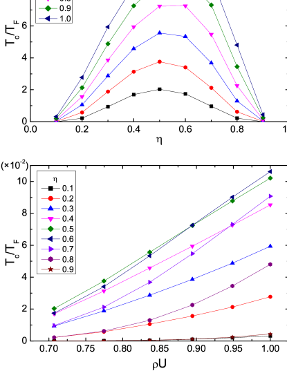
Figure 6: (Color online) Critical temperatures $T_{c}$ in unit of $T_{F}$ at different imbalance ratios ($\eta$) and coupling strengths ($\rho U$) in the intermediate coupling regime. The variation of $T_{c}$ with respect to $\rho U$ from the weak to the intermediate coupling regime is shown in Fig. 5.

We also calculated critical temperatures at different imbalance ratios with coupling strengths $\rho U\sim 1$ in the intermediate regime (see Fig. 6). For fixed coupling, the highest critical temperature appears near $\eta=0.5$ as expected and is about $10^{-2}T_{F}$ but also drops quickly as the imbalance ratio tends to zero or unity.

V Discussions and Summaries

We have shown that the population imbalance induced $p$-wave superfluid state may be observable in a 2D repulsive fermion gas. Population imbalance can be achieved by an unequal mixing of atoms in two hyperfine states, and tunable repulsive interactions can be realized by using the upper branch of a Feshbach resonance. In Ref.Jo et al. (2009), ${}^{6}\mathrm{Li}$ atoms in the repulsive regime were used to study the itinerant ferromagnetism. One problem that should be considered is that the upper branch of a Feshbach resonance is an excited branch, and will decay to the BEC molecule state due to inelastic three-body collisions Petrov (2003). However, with small scattering length and population imbalance, the decay rate is suppressed Jo et al. (2009); D’Incao and Esry (2005) and the system may be metastable for observation. For experimental observations, we suggest to look for rotational asymmetries in the momentum distribution or pairwise correlation in the time of flight expansion images of the dominant species Altman et al. (2004); Greiner et al. (2005). In addition, the transition temperature can be raised in two different ways (see Fig. 6). One is to adjust the imbalance ratio to the optimal value which is around $0.5$. As can be seen from Fig. 5, the theoretical transition temperature should be around $10^{-5}T_{F}\sim 10^{-3}T_{F}$ in the weak repulsive regime near the optimal imbalance ratio. Another one is to increase the coupling strength by Feshbach resonance. By extending our result to the intermediate coupling regime, we get an estimation of the critical temperature which reaches as high as $10^{-2}T_{F}$. Since our approach is asymptotically exact, the perturbative calculations are well controlled in the first stage of RG. After safely arriving at the second stage, where the cutoff $\Lambda$ is much smaller than the Fermi momentum $K_{F}$, the emergence of a large-N ensures the non-perturbative nature of the momentum shell RG in the second stage where a quantitatively calculation of critical temperature was given. However, for comparing with the experimental results, we should notice that another important issue is the trap effects on our system. In striking contrast with $s$-wave superfluid state, the trap asymmetries would have a strong influence on the spontaneously preferred orientation of $p$-wave superfluid state. We will study the trap effects in our future work.

In summary, we studied a possible new superfluid state for a 2D population imbalanced fermion gas with short-range repulsive interactions. This phenomena is different from the ones in the BEC-BCS crossover where the BEC molecule state is concerned. It is also different from the ones in the unitary region where the scattering length is approaching infinity and many universal properties emerge. For the system considered in this paper, the bare interaction is purely repulsive, and there are no intermediate bosons for inducing attractive interactions. We studied this system based on RG approach and treated different instabilities on an equal footing. There are no assumptions of specific orders compared with mean-field approach. What is essential for the Cooper instability is the mismatch of the Fermi surfaces caused by population imbalance in our system. It can also be achieved in mixture of fermions with unequal mass, to which our approach can be generalized straightforwardly. By working in the finite temperature formulism and numerically solving the flow equation, we gave a quantitatively calculation of the critical temperature. Our study is of particular significance both for probing $p$-wave superfluidity in the novel regime experimentally and for studying imbalanced fermionic systems with RG theory theoretically.