On a bifurcation value related
to quasi-linear Schrödinger equations

Abstract.

By virtue of numerical arguments we study a bifurcation phenomenon occurring for a class of minimization problems associated with the quasi-linear Schrödinger equation.

1. Introduction

Various physical situations are described by quasi-linear equations of the form

(1.1) $$\begin{cases}{\rm i}\phi_{t}+\Delta\phi+\phi\Delta|\phi|^{2}+|\phi|^{p-1}\phi=0&\text{in $(0,\infty)\times{\mathbb{R}}^{3}$},\\ \phi(0,x)=\phi_{0}(x)&\text{in ${\mathbb{R}}^{3}$},\end{cases}$$

where $1<p<11$, ${\rm i}$ stands for the imaginary unit and the unknown $\phi:(0,\infty)\times{\mathbb{R}}^{3}\to{\mathbb{C}}$ is a complex valued function. For example, it is used in plasma physics and fluid mechanics, in the theory of Heisenberg ferromagnets and magnons and in condensed matter theory. See e.g. the bibliography of  [6]. Motivated by the classical stability results of the semi-linear Schrödinger equation

(1.2) $$\begin{cases}{\rm i}\phi_{t}+\Delta\phi+|\phi|^{p-1}\phi=0&\text{in $(0,\infty)\times{\mathbb{R}}^{3}$},\\ \phi(0,x)=\phi_{0}(x)&\text{in ${\mathbb{R}}^{3}$},\end{cases}$$

namely the stability of ground states (least energy solutions of $-\Delta u+\omega u=|u|^{p-1}u$, $\omega>0$) for $1<p<\frac{7}{3}$ and their instability for $p\geq\frac{7}{3}$ (see [2, 5]), an interesting and physically relevant question for equation (1.1) is the orbital stability of ground state solutions of

(1.3) $$-\Delta u-u\Delta u^{2}+\omega u=|u|^{p-1}u\quad\text{in ${\mathbb{R}}^{3}$}.$$

When $1<p<\frac{13}{3}$, it is conjectured in [6] that the ground states are orbitally stable. However, in [6] this result was not proved. Instead, it was considered the stability issue for the minimizers of the problem

(1.4) $$\mathscr{M}(c)=\inf_{\begin{subarray}{c}u\in X\\ \|u\|_{L^{2}({\mathbb{R}}^{3})}^{2}=c\end{subarray}}{\mathscr{E}}(u),$$

where $1<p<\frac{13}{3}$ and the energy functional ${\mathscr{E}}$ defined on $X=\big{\{}u\in H^{1}({\mathbb{R}}^{3}):\,u|Du|\in L^{2}({\mathbb{R}}^{3})\big{\}}$ by

(1.5) $${\mathscr{E}}(u)=\frac{1}{2}\int_{{\mathbb{R}}^{3}}(1+2u^{2})|Du|^{2}dx-\frac{1}{p+1}\int_{{\mathbb{R}}^{3}}|u|^{p+1}dx.$$

This problem, which looks interesting by itself, can be seen as a useful tool for a first attempt towards the understanding of orbital stability of ground states of (1.3) for fixed $\omega>0$. Denoting by $\mathcal{G}(c)$ the set of solutions to (1.4), in [6] the authors prove that if $1<p<\frac{13}{3}$ and $c>0$ is such that $m(c)<0$, then ${\mathcal{G}}(c)$ is orbitally stable (see [6] for the definition). Concerning (1.4), we learn [6] that the following facts hold:

Proposition 1.1 (CJS, [6]).

The following properties hold.

1. Assume that $1<p<\frac{13}{3}$. Then $\mathscr{M}(c)>-\infty$ for every $c>0$.

2. Assume that $p=\frac{13}{3}$. Then $\mathscr{M}(c)>-\infty$ for $c>0$ small and $\mathscr{M}(c)=-\infty$ for $c>0$ large.

3. Assume that $\frac{13}{3}<p<11$. Then $\mathscr{M}(c)=-\infty$ for every $c>0$.

4. Assume that $1<p<\frac{13}{3}$ and let $c>0$ be such that $\mathscr{M}(c)<0$. Then problem (1.4) admits a positive minimizer $u_{c}\in X$ which is radially symmetric and radially decreasing. Moreover any solution $u_{c}\in X$ of (1.4) satisfies

   (1.6) $$-\Delta u_{c}-u_{c}\Delta u_{c}^{2}+\lambda_{c}u_{c}=|u_{c}|^{p-1}u_{c}$$

   for some $\lambda_{c}>0$.

5. Assume that $1<p<\frac{7}{3}$. Then $\mathscr{M}(c)<0$ for every $c>0$.

6. Assume that $\frac{7}{3}\leq p\leq\frac{13}{3}$. Then $\mathscr{M}(c)\leq 0$ for every $c>0$.

7. Assume that $\frac{7}{3}\leq p<\frac{13}{3}$. Then there exists

   $$c_{\sharp}=c(p)>0$$

   such that:

   1. If $c<c_{\sharp}$ then $\mathscr{M}(c)=0$ and $\mathscr{M}(c)$ does not admit a minimizer.

   2. If $c>c_{\sharp}$ then $\mathscr{M}(c)<0$ and $\mathscr{M}(c)$ admits a minimizer.

The motivation for the formulation of the following problems is mainly related to point (7) in the statement of Proposition 1.1. Notice that the value of $c_{\sharp}(p)$ can be characterized as follows

$$c_{\sharp}(p)=\inf\{c>0:\,\mathscr{M}(c)<0\},$$

This could help while trying to numerically compute the value of $c_{\sharp}(p)$. The bifurcation value $c_{\sharp}(p)$ which appears in the previous Proposition 1.1 is obtained in [6] by an indirect argument by contradiction and thus it is not explicitly available for calculation through a given formula. Hence, on these basis, it seems natural to formulate the following problems:

Problem 1.2.

Provide some lower and upper bounds of $\mathscr{M}(c)$ for $c>0$ and $p\in[\frac{7}{3},\frac{13}{3})$.

Problem 1.3.

Numerically compute or provide bounds for the map $c_{\sharp}:[\frac{7}{3},\frac{13}{3})\to(0,+\infty)$.

Problem 1.4.

Numerically compute the solutions to $\mathscr{M}(c)$ for $c>c_{\sharp}(p)$ with $p\in[\frac{7}{3},\frac{13}{3})$.

For the corresponding, more classical [5], semi-linear minimization problem

$$\mathscr{M}_{{\rm sl}}(c)=\inf_{\begin{subarray}{c}u\in H^{1}({\mathbb{R}}^{3})\\ \|u\|_{L^{2}({\mathbb{R}}^{3})}^{2}=c\end{subarray}}{\mathscr{E}}_{{\rm sl}}(u),\qquad{\mathscr{E}}_{{\rm sl}}(u)=\frac{1}{2}\int_{{\mathbb{R}}^{3}}|Du|^{2}dx-\frac{1}{p+1}\int_{{\mathbb{R}}^{3}}|u|^{p+1}dx,\quad 1<p<\frac{7}{3},$$

there is no bifurcation phenomena, namely $c_{\sharp}(p)=0$ for every $1<p<\frac{7}{3}$ and Problem 1.4 was studied in [4] by arguing on a suitable associated parabolic problem in order to decrease initial energies computed on Gaussian initial guesses. An important point both for analytical and numerical purposes is the fact that minimizers of $\mathscr{M}_{{\rm sl}}(c)$ have fixed sign, are radially symmetric, decreasing and unique, up to translations and multiplications by $\pm 1$. In principle, the uniqueness is used in [4] to justify that the numerical algorithm really provides the solution to the minimization problem $\mathscr{M}_{{\rm sl}}(c)$. To show the uniqueness of solutions to $\mathscr{M}_{{\rm sl}}(c)$ one can argue as follows. By the result of [9], for any $\lambda>0$ there exists a unique (up to translations) positive and radially symmetric solution $r=r_{\lambda}:{\mathbb{R}}^{3}\to{\mathbb{R}}$ of

$$-\Delta r+\lambda r=r^{p}\qquad\text{in ${\mathbb{R}}^{3}$},$$

In turn, given $\lambda_{1},\lambda_{2}>0$, if $r_{1},r_{2}:{\mathbb{R}}^{3}\to{\mathbb{R}}$ denote, respectively, positive radial solutions of

(1.7) $$-\Delta r_{1}+\lambda_{1}r_{1}=r_{1}^{p}\qquad\text{in ${\mathbb{R}}^{3}$},\qquad\,\,\,-\Delta r_{2}+\lambda_{2}r_{2}=r_{2}^{p}\qquad\text{in ${\mathbb{R}}^{3}$},$$

there exists some point $\xi\in{\mathbb{R}}^{3}$ such that

(1.8) $$r_{2}(x+\xi)=\mu r_{1}(\gamma x),\qquad\gamma:=\Big{(}\frac{\lambda_{2}}{\lambda_{1}}\Big{)}^{\frac{1}{2}},\quad\mu:=\Big{(}\frac{\lambda_{2}}{\lambda_{1}}\Big{)}^{\frac{1}{p-1}}.$$

Let now $r_{1}$ and $r_{2}$ be two given solutions to the minimization problem $\mathscr{M}_{{\rm sl}}(c)$ and let $-\lambda_{1}$ and $-\lambda_{2}$ be the corresponding Lagrange multipliers. By virtue of [5, Theorem II.1, ii)], $\lambda_{1},\lambda_{2}>0$ and $r_{1},r_{2}$ are $C^{2}$ solutions of (1.7), are radially symmetric, radially decreasing and with fixed sign. In turn, up to multiplication by $\pm 1$, $r_{1},r_{2}>0$ and by (1.8) it holds

$$c=\|r_{2}\|_{L^{2}({\mathbb{R}}^{3})}^{2}=\|r_{2}(\cdot+\xi)\|_{L^{2}({\mathbb{R}}^{3})}^{2}=\mu^{2}\gamma^{-3}\int_{{\mathbb{R}}^{3}}r_{1}^{2}(x)dx=c\mu^{2}\gamma^{-3},$$

yielding in turn $\mu^{2}\gamma^{-3}=1$. By the definition of $\gamma$ and $\mu$ in (1.8), we get $\lambda_{1}=\lambda_{2}$ and $\gamma=\mu=1$, yielding from (1.8) as desired $r_{1}=r_{2}$, up to a translation.

On the contrary, it is not currently known that minimizers $r\in X$ of the quasi-linear minimization problem (1.4) are unique, up to translations and multiplications by $\pm 1$, although it is conjectured that this is the case. If $r\in X$ is a given minimizer for (1.4), arguing as in [6] it is possible to prove that it has fixed sign, so that, up to multiplication by $-1$, we may assume $r>0$. Then, $r$ is radially symmetric and radially decreasing, see for instance the main result of [12]. Given $r_{1}$ and $r_{2}$ two solutions to the minimization problem $\mathscr{M}(c)$ we have that $-\lambda_{1}$ and $-\lambda_{2}$ are the corresponding Lagrange multipliers and $\lambda_{1},\lambda_{2}>0$ in light of [6, Lemma 4.6]

(1.9) $$-\Delta r_{i}-r_{i}\Delta r_{i}^{2}+\lambda_{i}r_{i}=r_{i}^{p}\qquad\text{in ${\mathbb{R}}^{3}$},\qquad i=1,2.$$

With respect to the semi-linear case, the main problem is the identification of Lagrange multipliers, which cannot be inferred as in the semi-linear case. In fact, let us consider as above the rescaling for $r_{1}$ by

$$w(x)=\mu r_{1}(\gamma x),\qquad\gamma:=\Big{(}\frac{\lambda_{2}}{\lambda_{1}}\Big{)}^{\frac{1}{2}},\quad\mu:=\Big{(}\frac{\lambda_{2}}{\lambda_{1}}\Big{)}^{\frac{1}{p-1}}.$$

Then this yields $\|w\|_{L^{2}({\mathbb{R}}^{3})}^{2}=(\lambda_{2}/\lambda_{1})^{\frac{4-3(p-1)}{2(p-1)}}c$ and

$$-\Delta w-(\lambda_{1}/\lambda_{2})^{\frac{2}{p-1}}w\Delta w^{2}+\lambda_{2}w=w^{p}\qquad\text{in ${\mathbb{R}}^{3}$}.$$

Although there are recent uniqueness results for the positive radial solutions to (1.9), due to the presence of the residual coefficient $(\lambda_{1}/\lambda_{2})^{2/(p-1)}$, we cannot infer as before that $w(\cdot)=r_{2}(\cdot+\xi)$ for some point $\xi\in{\mathbb{R}}^{3}$. In the course of the next section, we shall compute the ground state under a conjectured property (indeed true in the semi-linear case discussed above) stated in the following

Conjecture 1.5.

Assume that $r_{1},r_{2}>0$ are radial decreasing solutions to (1.9) with $\lambda_{1},\lambda_{2}>0$, ${\mathcal{E}}(r_{i})<0$ and $\|r_{i}\|^{2}_{L^{2}({\mathbb{R}}^{3})}=c$ for $i=1,2$. Then $\lambda_{1}=\lambda_{2}$ and $r_{2}=r_{1}(\cdot+\xi)$, for some $\xi\in{\mathbb{R}}^{3}$.

Consequently, given $c>0$, assume that there exist $r:{\mathbb{R}}^{3}\to{\mathbb{R}}$ and $\lambda>0$ such that

$$\text{$r=\rho(|x|)>0$,\,\, $\rho^{\prime}\leq 0$},\qquad\|r\|^{2}_{L^{2}({\mathbb{R}}^{3})}=c,\qquad{\mathcal{E}}(r)<0,\qquad-\Delta r-r\Delta r^{2}+\lambda r=r^{p}\quad\text{in ${\mathbb{R}}^{3}$}.$$

We know that this happens to be the case under the assumption that $\mathscr{M}(c)<0$. Then $r$ is the unique solution to problem $\mathscr{M}(c)$, up to translations and multiplication by $\pm 1$. In figure 1, we compared the shape of the solutions to

(1.10) $$\mathscr{M}_{\vartheta}(70):=\inf_{\begin{subarray}{c}u\in X\\ \|u\|_{L^{2}({\mathbb{R}}^{3})}^{2}=70\end{subarray}}{\mathscr{E}}_{\vartheta}(u),\qquad{\mathscr{E}}_{\vartheta}(u):=\frac{1}{2}\int_{{\mathbb{R}}^{3}}(1+2\vartheta u^{2})|Du|^{2}dx-\frac{1}{3}\int_{{\mathbb{R}}^{3}}|u|^{3}dx.$$

with $\vartheta=1$ (quasi-linear case) and $\vartheta=0$ (semi-linear case). Roughly speaking, the term $-u\Delta u^{2}$ produces an additional diffusive contribution which tends to squeeze the bump down against source effects.

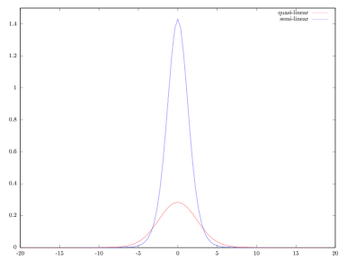
Figure 1. Comparison between the solution (a section of the absolute value squared) of (1.10) with $\vartheta=1$ (quasi-linear case) and with $\vartheta=0$ (semi-linear case). The additional diffusive term present in the quasi-linear case tends to produce squeezing effects.

2. Results

Concerning Problem 1.2, we have the following (see also Fig. 2)

Proposition 2.1.

The following properties hold.

1. For every $\frac{7}{3}\leq p<\frac{13}{3}$ there holds

   $$\forall c>0:\quad\mathscr{M}(c)\leq\inf_{\sigma>0}\Big{(}\sigma^{2}\frac{3c}{4}+\sigma^{5}\frac{3c^{2}}{8\sqrt{2}\pi^{3/2}}-\sigma^{\frac{3(p-1)}{2}}\frac{2\sqrt{2}c^{\frac{p+1}{2}}\pi^{\frac{3}{2}-\frac{3(p+1)}{4}}}{(p+1)^{\frac{5}{2}}}\Big{)}.$$

2. For every $\frac{7}{3}\leq p<\frac{13}{3}$, if

   $${\mathcal{K}}_{p}:=4^{\frac{3p-3}{10}}S_{{\rm sob}}^{\frac{3p-3}{5}},\qquad S_{{\rm sob}}=\frac{2^{1/3}}{\sqrt{3\pi}}\frac{1}{\Gamma^{1/3}(3/2)},$$

   being $S_{{\rm sob}}$ the best Sobolev constant for the embedding of $H^{1}({\mathbb{R}}^{3})$ into $L^{q}({\mathbb{R}}^{3})$, there holds

   $$\forall c>0:\quad\mathscr{M}(c)\geq-\frac{13-3p}{3(p-1)}\Big{(}\frac{10(p+1)}{3(p-1){\mathcal{K}}_{p}}\Big{)}^{\frac{10}{3p-13}}c^{\frac{11-p}{13-3p}}.$$

3. For $p=\frac{7}{3}$, setting $A:=\frac{2\sqrt{2}3^{5/2}}{10^{5/2}\pi}$, $B:=\frac{3^{2/3}}{2^{7/3}\pi}$ and $c_{\sharp}:=(\frac{10^{5/2}\pi}{2^{7/2}3^{3/2}})^{3/2}$, there holds

   $$\forall c>0:\quad\mathscr{M}(c)|_{p=\frac{7}{3}}\leq\begin{cases}\,\,\,0&\text{if $c\leq c_{\sharp}$,}\\ -\big{[}\big{(}\frac{2}{5}\big{)}^{2/3}-\big{(}\frac{2}{5}\big{)}^{5/3}\big{]}\frac{[Ac^{5/3}-3c/4]^{5/3}}{Bc^{4/3}}&\text{if $c\geq c_{\sharp}$.}\end{cases}$$

   In particular, $\mathscr{M}(c)|_{p=\frac{7}{3}}\apprle-Mc^{13/9},$ for every $c>0$ large and some $M>0$.

4. If $p=\frac{13}{3}$, setting

   $$c_{\flat}:=(16/{3{\mathcal{K}}_{\frac{13}{3}}})^{3/2}\approx 19.73,\qquad{\mathcal{K}}_{\frac{13}{3}}:=4S_{{\rm sob}}^{2},$$

   we have $\mathscr{M}(c)=0$ for every $c\leq c_{\flat}$ and the infimum $\mathscr{M}(c)$ is not attained.

5. If $p=\frac{13}{3}$, setting

   $$c^{\flat}:=\frac{3^{3/2}(16/3)^{15/4}\pi^{3/2}}{32^{3/2}}\approx 85.09,$$

   we have $\mathscr{M}(c)=-\infty$ for every $c>c^{\flat}$.

Proof.

Properties (1), (3) and (5) easily follow by the arguments in Section 3 and direct computations. Properties (2) and (4) need bounds from below and can be justified as follows. The best Sobolev constant $S_{{\rm sob}}$ is computed through the formula contained in [13]. Concerning (4), by Hölder and Sobolev inequalities, for $u\in X$ we have

(2.1) $$\int_{{\mathbb{R}}^{3}}|u|^{16/3}dx\leq\Big{(}\int_{{\mathbb{R}}^{3}}|u|^{2}dx\Big{)}^{2/3}\Big{(}\int_{{\mathbb{R}}^{3}}|u|^{12}dx\Big{)}^{1/3}\leq{\mathcal{K}}_{\frac{13}{3}}c^{2/3}\Big{(}\int_{{\mathbb{R}}^{3}}|u|^{2}|Du|^{2}dx\Big{)},$$

where we have used the fact that ($2^{*}=6$ is the critical Sobolev exponent in ${\mathbb{R}}^{3}$)

$$\int_{{\mathbb{R}}^{3}}|u|^{12}dx=\int_{{\mathbb{R}}^{3}}(u^{2})^{2^{*}}dx,\qquad\int_{{\mathbb{R}}^{3}}|D(u^{2})|^{2}dx=4\int_{{\mathbb{R}}^{3}}|u|^{2}|Du|^{2}dx.$$

From inequality (2.1) we infer

$${\mathcal{E}}(u)\geq\int_{{\mathbb{R}}^{3}}|u|^{2}|Du|^{2}dx-\frac{3{\mathcal{K}}_{\frac{13}{3}}}{16}c^{2/3}\int_{{\mathbb{R}}^{3}}|u|^{2}|Du|^{2}dx,$$

which yields ${\mathcal{E}}(u)\geq 0$ for every $u\in X$ and any $c\leq c_{\flat}$ and hence, in turn, the desired conclusion. In a similar fashion, concerning (2), if $p<13/3$, using Hölder and Sobolev inequalities for any $u\in X$ we have

(2.2) $$\int_{{\mathbb{R}}^{3}}|u|^{p+1}dx\leq{\mathcal{K}}_{p}c^{\frac{11-p}{10}}\Big{(}\int_{{\mathbb{R}}^{3}}|u|^{2}|\nabla u|^{2}dx\Big{)}^{\frac{3p-3}{10}},$$

yielding immediately that

$${\mathcal{E}}(u)\geq\int_{{\mathbb{R}}^{3}}|u|^{2}|\nabla u|^{2}dx-\frac{{\mathcal{K}}_{p}}{p+1}c^{\frac{11-p}{10}}\Big{(}\int_{{\mathbb{R}}^{3}}|u|^{2}|\nabla u|^{2}dx\Big{)}^{\frac{3p-3}{10}}.$$

Since $p<3/13$ it follows that $\frac{3p-3}{10}<1$. In turn, the function $\omega:[0,+\infty)\to{\mathbb{R}}$

$$\omega(s)=s-\frac{{\mathcal{K}}_{p}}{p+1}c^{\frac{11-p}{10}}s^{\frac{3p-3}{10}},\qquad s\geq 0,$$

always admits a (negative) absolute minimum point at a point $t_{p,c}>0$ which can be easily computed, yielding the desired assertion by the arbitrariness of $u\in X$. ∎

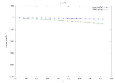
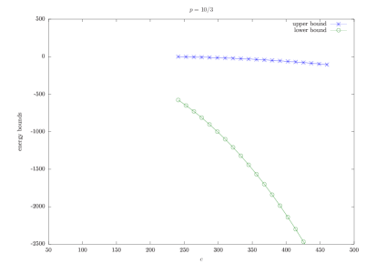
Figure 2. Upper and lower bounds of ${\mathscr{M}}(c)$ according to the estimates obtained Proposition 2.1 in the particular cases $p=7/3$ (sharp bounds) and $p=10/3$ (less sharp bounds).

Concerning Problem 1.3 we shall provide an upper bounding profile for the values of $c_{\sharp}(p)$ and give indications showing that very likely $c_{\sharp}(p)$ remains in a small lower neighborhood of this profile. As $p$ increases from $7/3$ up to a certain value $p_{0}\sim 3.3$ the bounding profile is increasing, reaching values around $c=250$. Then, after $p_{0}$ it decreases. Concerning Problem 1.4, under the conjectured uniqueness result we compute the ground state solutions for some values of $c$ greater than the upper bounding profile for the values of $c_{\sharp}(p)$. In the case $c<c_{\sharp}(p)$, roughly speaking, if $(u_{n})\subset X$ is an arbitrary minimizing sequence for problem $\mathscr{M}(c)$, since we know that $\mathscr{M}(c)$ is not attained, $(u_{n})$ cannot be strongly convergent, up to a subsequence, in $L^{2}({\mathbb{R}}^{3})$ and in turn in $H^{1}({\mathbb{R}}^{3})$. Then, by virtue of Lions’s compactness-concentration principle, only vanishing or dichotomy might occur, in the language of [10, 11]. On the other hand, it was proved in [6, Theorem 1.11] that dichotomy can always be ruled out. In conclusion, the only possibility remaining for a minimizing sequence is vanishing, precisely:

$$\mbox{for every $R>0$:}\qquad\lim_{n\to\infty}\sup_{y\in{\mathbb{R}}^{3}}\int_{B(y,R)}u_{n}^{2}dx=0,$$

where $B(y,R)$ denotes the ball in ${\mathbb{R}}^{3}$ of center $y$ and radius $R$. In particular, fixed any bounded domain $C$ in ${\mathbb{R}}^{3}$, imagined for instance as the computational domain, the sequence $(u_{n})$ cannot be essentially supported into $C$, being for $R_{0}={\rm diam}(C)$

$$\int_{{\mathbb{R}}^{3}\setminus C}u_{n}^{2}dx\geq c-\sup_{y\in C}\int_{B(y,R_{0})}u_{n}^{2}dx\geq c-\sup_{y\in{\mathbb{R}}^{3}}\int_{B(y,R_{0})}u_{n}^{2}dx\geq c/2,$$

for $n$ sufficiently large. This means that $(u_{n})$ (in particular any numerically approximating ${\mathscr{M}}(c)$) tends to spread out of any fixed (computational) domain $C$. For instance, the sequence $(g_{c,\sigma_{j}})$ with $\sigma_{j}\to 0$ as $j\to\infty$, where $g_{c,\sigma}$ is defined in Section 3 is such that $\|g_{c,\sigma_{j}}\|_{L^{2}({\mathbb{R}}^{3})}^{2}=c$ and ${\mathcal{E}}(g_{c,\sigma_{j}})\to 0$ as $j\to\infty$ and hence, for $c<c_{\sharp}(p)$, being ${\mathscr{M}}(c)=0$, it is a minimization sequence. It shows vanishes, since

$$\sup_{y\in{\mathbb{R}}^{3}}\int_{B_{R}(y)}g_{c,\sigma_{j}}^{2}dx\leq CR^{3}\sigma_{j}^{3},$$

for all $R>0$ and $j\geq 1$.

3. Numerical approximation

Instead of a direct minimization of the energy functional (1.5) (see, for instance, [3]), as seen in [1, 4], it is also possible to find a solution of (1.6) by solving the parabolic problem

(3.1) $$\left\{\begin{aligned} \partial_{t}u&=\Delta u+u\Delta u^{2}+|u|^{p-1}u-\lambda(u)u\\ u(0)&=u_{0},\quad\|u_{0}\|^{2}_{L^{2}({\mathbb{R}}^{3})}=c\end{aligned}\right.$$

up to the steady-state $u_{c}$, where $\lambda(u)$ is defined by

$$\lambda(u)=-\frac{\int_{{\mathbb{R}}^{3}}(1+4u^{2})|Du|^{2}-\int_{{\mathbb{R}}^{3}}|u|^{p+1}}{\int_{{\mathbb{R}}^{3}}u^{2}}$$

This approach in known as continuous normalized gradient flow. It is easy to show that the energy associated to the solution $u(t)$ decreases in time, whereas the $L^{2}$-norm is constant.

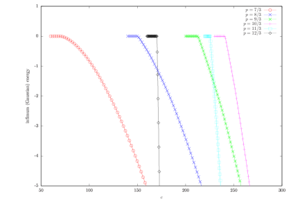
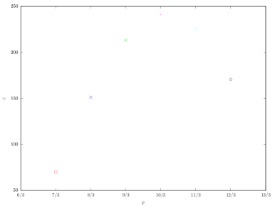
Figure 3. Values of the infimum (Gaussian) energy with respect to $c$ (left) and values of $c_{\mathrm{g}}$ (right): from $p=7/3$ to $p=12/3$ they are $69.510$, $150.65$, $212.91$, $241.01$, $225.42$, $170.33$, respectively.

In order to find a “good” initial solution $u_{0}$, that is a function with a negative energy, we can consider the family of Gaussian radial functions

$$g_{c,\sigma}(r)=\frac{\sqrt{c\sigma^{3}}}{\sqrt[4]{\pi^{3}}}e^{-\sigma^{2}r^{2}/2},\quad\|g_{c,\sigma}\|^{2}_{L^{2}({\mathbb{R}}^{3})}=c,\quad\sigma>0$$

and minimize the energy $\mathscr{E}(g_{c,\sigma})$, which, for a given $p$ and $c$, can be computed analytically as

(3.2) $$\mathscr{E}(g_{c,\sigma})=\sigma^{2}\frac{3c}{4}+\sigma^{5}\frac{3c^{2}}{8\sqrt{2}\pi^{3/2}}-\sigma^{\frac{3(p-1)}{2}}\frac{2\sqrt{2}c^{\frac{p+1}{2}}\pi^{\frac{3}{2}-\frac{3(p+1)}{4}}}{(p+1)^{\frac{5}{2}}}$$

with respect to the parameter $\sigma$. If the infimum value for the energy is zero, we increase the value of $c$ and look again for the infimum energy. We proceed with increasing values of $c$ until we find a $c_{\mathrm{g}}$ such that the minimum energy with respect to $\sigma$, corresponding to a value $\bar{\sigma}$, is negative. This is possible, since we consider a discrete sequence of increasing values for $c$ in order to test the negativity of the energy. Such a $c_{\mathrm{g}}$ is clearly an upper bound for the desired value $c_{\sharp}$. For the range $p=7/3,8/3,9/3,10/3,11/3,12/3$ we obtain the values reported in Figure 3 (right).

Now, we are ready to look for values $c<c_{\mathrm{g}}$, for which the steady-state of (3.1) has a negative energy. To this purpose, we choose $u_{0}=g_{c,\sigma}$, where $\sigma=\bar{\sigma}\cdot c/c_{\mathrm{g}}$. The meaning of this choice is the following: since $c<c_{\mathrm{g}}$, the infimum value of the energy attained by a Gaussian function is zero and corresponds to the limit case $\sigma\to 0$. We instead select $0<\sigma<\bar{\sigma}$ with the idea that $g_{c,\sigma}$ is a good initial value, because close to $g_{c_{\mathrm{g}},\bar{\sigma}}$, that is the optimal element in the Gaussian family. With this choice, clearly we have $\mathscr{E}(u_{0})>0$.

In order to fix once and for all the computational domain in such a way that it does not depend on $\sigma$, we scale the space variables by $\sigma$ and the unknown $u$ in order to have unitary $L^{2}$ norm, that is

$$\sqrt{c\sigma^{3}}v_{c}(t,\sigma\cdot)=u(t,\cdot)$$

We end up with

(3.3) $$\left\{\begin{aligned} \partial_{t}v_{c}&=\sigma^{2}\Delta v_{c}+c\sigma^{5}v_{c}\Delta v_{c}^{2}+(c\sigma^{3})^{\frac{p-1}{2}}|v_{c}|^{p-1}v_{c}+\eta(v_{c})v_{c}\\ v_{c}(0)&=\frac{1}{\sqrt[4]{\pi^{3}}}e^{-r^{2}/2}\end{aligned}\right.$$

where

$$\eta(v_{c})=\frac{\int_{{\mathbb{R}}^{3}}\sigma^{2}(1+4c\sigma^{3}v_{c}^{2})|Dv_{c}|^{2}-(c\sigma^{3})^{\frac{p-1}{2}}\int_{{\mathbb{R}}^{3}}|v_{c}|^{p+1}}{\int_{{\mathbb{R}}^{3}}v_{c}^{2}}$$

The corresponding energy is

$$\mathscr{E}(u)=E(v_{c})=\frac{1}{2}\int_{{\mathbb{R}}^{3}}c\sigma^{2}(1+2c\sigma^{3}v_{c}^{2})|Dv_{c}|^{2}-\frac{c(c\sigma^{3})^{\frac{p-1}{2}}}{p+1}\int_{{\mathbb{R}}^{3}}|v_{c}|^{p+1}.$$

We solve equation (3.3) up to a final time $T$ for which

$$\|\bar{\sigma}^{2}\Delta v_{c}+c\bar{\sigma}^{5}v_{c}\Delta v_{c}^{2}+(c\bar{\sigma}^{3})^{\frac{p-1}{2}}|v_{c}|^{p-1}v_{c}+\eta(v_{c})v_{c}\|_{L^{2}({\mathbb{R}}^{3})}<\mathrm{tol}$$

where $\mathrm{tol}$ is a prescribed tolerance to detect the approximated steady-state. As already done in [4], we apply the exponential Runge–Kutta method of order two (see [8]) to the spectral Fourier decomposition in space of (3.3). The embedded exponential Euler method gives the possibility to derive a variable stepsize integrator, which is particularly useful when approaching the steady-state solution, allowing the time steps to become larger and larger. For our numerical experiments, we used the computational domain $[-5,5]^{3}$, the regular grid of $64^{3}$ points, a tolerance for the local error (in the $L^{2}$ norm) equal to $10^{-8}$ and the steady-state detection tolerance $\mathrm{tol}=10^{-7}$.

The solution $v_{c}(T)$ is then considered an approximated steady-state solution. If its energy is negative and it is radially symmetric and decreasing, then we conclude it is a minimum for $\mathscr{M}(c)$. Therefore, $c\geq c_{\sharp}$ is the current upper bound for $c_{\sharp}$ (blue circle in Figure 4).

On the other hand, if $c<c_{\sharp}$, then $\mathscr{M}(c)=0$ and the infimum is approximated by flatter and flatter functions. This is perfectly clear in the case one restricts the search among Gaussian functions, for which $\mathscr{E}(g_{c,\sigma})\to 0$ for $\sigma\to 0$. This situation can be recognized in the numerical experiments because the essential support of $v_{c}(t)$ during time evolution tends to grow and to spread out the computational domain (green plus in Figure 4), which was chosen in such a way to comfortably contain the essential support of the initial solution $v_{c}(0)$. In this case, we apply a bisection algorithm on the values $c$ and $c_{\mathrm{g}}$ (the Gaussian upper bound for $c_{\sharp}$) in order to find a tighter upper bound for $c_{\sharp}$, since $c<c_{\sharp}$ and $c_{\mathrm{g}}\geq c_{\sharp}$.

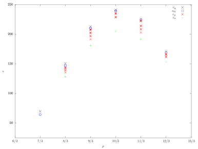
Figure 4. Values of $c_{\mathrm{g}}$ (Gaussian upper bound of $c_{\sharp}$), $c_{\mathrm{m}}$ (values for which $E(v_{c_{\mathrm{m}}}(T))<0$) and $c_{\mathrm{p}}$ (values for which $E(v_{c_{\mathrm{p}}}(T))>0$). For instance, for the case $p=9/3$ and $c=0.9875\cdot c_{\mathrm{g}}\approx 210.25$ we found an approximated steady-state with energy $E(v_{c}(T))\approx-1.30\cdot 10^{-1}$ (blue circle), whereas with $c=0.975\cdot c_{\mathrm{g}}\approx 207.59$, we found an approximated steady-state with energy $E(v_{c}(T))\approx 6.97\cdot 10^{-2}$ (red star).

In the numerical experiments we encountered another situation: starting from an initial solution with positive energy, it was possible to find a radially symmetric and decreasing approximated steady-state solution, whose support was perfectly contained into the computational domain and with a positive energy (red star in Figure 4). This solution is not a solution with minimum energy, because for $\sigma$ small enough it is possible to find a Gaussian function $g_{c,\sigma}$ with smaller energy. In our numerical experiments, we observed this behaviour, for a given $p$ and with the tolerances described above, for the values of $c$ between the first value for which the essential support of the solution spread out the computational domain and the current upper bound for $c_{\sharp}$. We notice that we were not able to obtain solutions with positive energy in the limit case $p=7/3$.

Overall, from the numerical experiments we found out that the higher is $p$ the more difficult is to find a value of $c<c_{\mathrm{g}}$ for which the steady-state has a negative energy and can thus be considered a solution of minimum energy.

References

[1]W. Bao, Q. Du,
Computing the ground state solution of Bose–Einstein condensates by a
normalized gradient flow,
SIAM J. Sci. Comput.25 (2004), 1674–1697.
[2]H. Berestycki, T. Cazenave,
Instabilité des états stationnaires dans les équations de Schrödinger et de
Klein-Gordon non linéaire,
C. R. Acad. Sci. Paris293 (1981), 489–492.
[3]M. Caliari, A. Ostermann, S. Rainer, M. Thalhammer,
A minimisation approach for computing
the ground state of Gross–Pitaevskii systems,
J. Comput. Phys.228 (2009), 349–360.
[4]M. Caliari, M. Squassina,
Numerical computation of soliton dynamics for NLS equations in a driving potential,
Electron. J. Differential Equations89 (2010), 1–12.
[5]T. Cazenave, P.L. Lions,
Orbital stability of standing waves for some nonlinear Schrödinger equations,
Comm. Math. Phys.85 (1982), 549–561.
[6]M. Colin, L. Jeanjean, M. Squassina,
Stability and instability results for standing waves of quasi-linear Schrödinger equations,
Nonlinearity23 (2010), 1353–1385.
[7]F. Gladiali, M. Squassina,
Uniqueness of ground states for a class of quasi-linear elliptic equations
Adv. Nonlinear Anal., to appear.
[8]M. Hochbruck, A. Ostermann,
Exponential Integrators,
Acta Numerica19 (2010), 209–286.
[9]M.K. Kwong,
Uniqueness of positive solutions of in ,
Arch. Rational Mech. Anal.105 (1989), 243–266.
[10]P.L. Lions, The concentration-compactness principle in the
calculus of variations. The locally compact case. I., Ann. Inst. H. Poincaré Anal. Non Linéaire1 (1984),
109–145.
[11]P.L. Lions, The concentration-compactness principle in the
calculus of variations. The locally compact case. II., Ann. Inst. H. Poincaré Anal. Non Linéaire1 (1984),
223–283.
[12]M. Squassina,
On the symmetry of minimizers in constrained quasi-linear problems,
Adv. Calc. Var.4 (2011), 339–362.
[13]G. Talenti,
Best constant in Sobolev inequality,
Ann. Mat. Pura Appl.110 (1976), 353–372.