Equation of state for partially ionized carbon and oxygen mixtures at high temperatures

Abstract

The equation of state (EOS) for partially ionized carbon, oxygen, and carbon-oxygen mixtures at temperatures $3\times 10^{5}\mbox{~{}K}\lesssim T\lesssim 3\times 10^{6}$ K is calculated over a wide range of densities, using the method of free energy minimization in the framework of the chemical picture of plasmas. The free energy model is an improved extension of our model previously developed for pure carbon (Phys. Rev. E 72, 046402). The internal partition functions of bound species are calculated by a self-consistent treatment of each ionization stage in the plasma environment taking into account pressure ionization. The long-range Coulomb interactions between ions and screening of the ions by free electrons are included using our previously published analytical model, recently improved, in particular for the case of mixtures. We also propose a simple but accurate method of calculation of the EOS of partially ionized binary mixtures based on detailed ionization balance calculations for pure substances.

I Introduction

An understanding of the physical properties of matter at high densities and temperatures is important as a problem of fundamental physics as well as for various applications. A particularly challenging problem is the calculation of the equation of state (EOS) for stellar partial ionization zones, where the electrons and the different ionic species cannot be regarded as simple mixtures of ideal gases: Coulomb interactions, bound-state level shifts, pressure ionization, and electron degeneracy must be taken into account. In a previous publication Potekhin et al. (2005), we calculated the EOS for carbon at temperatures $10^{5}\mbox{~{}K}\lesssim T\lesssim 10^{7}$ K over a wide range of densities $\rho$, based on the free energy minimization method (Harris et al., 1960; Graboske et al., 1969) which enables us to include the complex physics in the model and ensures thermodynamic consistency. For the case of carbon, in particular, the EOS developed by Fontaine et al. Fontaine et al. (1977) (FGV) more than three decades ago and widely used in astrophysics up to now is based on the free energy minimization method at relatively low densities $\rho\lesssim 0.1$ g cm^-3.

The free energy model inevitably becomes complicated when density increases above $\rho\gtrsim 0.1$ g cm^-3 because of the growing importance of nonideal contributions and the onset of pressure ionization. This latter phenomenon is difficult to treat in the framework of the “chemical picture” of plasmas, which assumes that the different ion species retain their identity (see, e.g., Refs. Saumon et al. (1995); Potekhin (1996); Rogers (2000), for discussions). On the other hand, EOS calculations within the more rigorous “physical picture”, quite successful at relatively low $\rho$ (e.g., Rogers et al. (1996)), become prohibitively complicated at high densities. First principle approaches based on path integral Monte Carlo (PIMC) Militzer & Ceperley (2000); Bezkrovniy et al. (2004) or molecular dynamics (MD) calculations Surh et al. (2001); Mazevet et al. (2003) are computationally highly expensive, especially at high temperatures when excited ionic cores should be considered. To the best of our knowledge, no PIMC or MD data for carbon or oxygen in the temperature-density range of interest in this paper has been published so far.

Besides these first principle based computations and a few works that consider the influence of anisotropic distributions of neighboring ions (e.g. Refs. Nardi (1990); Wilson et al. (2011)), hot dense plasma studies of medium- to high-$Z$ elements are generally built around the modeling of an ion in its plasma environment placing it at the center of a spherically symmetric system. The complexity of the physics that is still required leads to a wealth of models. In ion sphere (IS) models Liberman (1979) neighboring ions act as a mere neutralizing background beyond some radius, while some correlation with the central ion can be introduced through the computation of pair distribution functions Blancard & Faussurier (2004), for instance in the hypernetted chain approximation (HNC) Wünsch et al. (2009). The free electron background may be obtained from model prescriptions like Thomas-Fermi Feynman et al. (1949); Kirzhnits & Shpatakovskaya (1995) or may involve quantum computations, usually from the Kohn-Sham equations in the density functional theory (DFT) context Piron et al. (2009); Pattison et al. (2010). Several levels of refinement are possible to model the atomic structure of the central ion. Most of them merge the various excitation and/or ionization states into a fictitious average atom (AA) Rozsnyai (1972). This saves a lot of computation time because the overall self-consistent scheme for the ion and its environment has to be solved only once for a given thermodynamics condition. The price to pay, especially when interested in opacities, is some additional statistical procedure to infer individual ionization stages populations from the average-atom solution (e.g. Pain et al. (2006)). This undoubtedly works well for high-$Z$ elements due to their innumerable quantum states which translate into unresolved transition arrays (UTA), but for lighter elements such as carbon or oxygen the relevance of the AA scheme becomes questionable.

In this paper we employ a generalized version of the EOS model Potekhin et al. (2005) which relies on the free energy minimization in the framework of the chemical picture and is applied to high densities across the pressure ionization region. We combine separate models for different ionization stages in the plasma environment, taking into account the detailed structure of bound states (configurations, $LS$ terms), and use Boltzmann statistics to sum up the internal partition functions of these ions. The atomic structure of each ion embedded in the dense plasma is calculated using a scheme (Massacrier, 1994) which self-consistently takes into account the modification of bound states due to the environment. The free electron density around each ion is treated quantum mechanically, thus resolving the resonances. Though neighboring ions act at this level as a neutralizing background, the long-range interactions in the system of charged particles (ions and electrons) is included in the thermodynamics using the theory previously developed for fully ionized plasmas (see Ref. (Potekhin and Chabrier, 2010) and references therein). This model allows us to obtain not only the thermodynamic functions, but also directly number fractions for every ionization stage, unlike AA models.

As different ions are treated on an equal footing, whether from the same element or not, our approach allows to treat mixtures in a similar way as pure plasmas. We apply the model to carbon and oxygen plasmas at temperatures between $3\times 10^{5}$ K and $3\times 10^{6}$ K and mass densities in the range $10^{-3}$ g cm^-3 $\lesssim\rho\lesssim 10^{4}$ g cm^-3. We also consider carbon-oxygen mixtures at the same plasma parameter values and propose a simple but accurate method of calculation of thermodynamic functions of the mixtures based on the solution of the ionization equilibrium problem for the pure substances. At $T\lesssim 3\times 10^{5}$ K the model remains valid in principle, but the calculation becomes numerically much more difficult in the current implementation, and it has not been realized in this work. For temperatures higher than $\simeq 3\times 10^{6}$ K our model recovers a simpler one where the free electron density is assumed to be uniform.

In Sec. II we briefly describe the total free energy model. In Sec. III we present the model for internal free energy of ions, which takes into account bound state configurations in $LS$ coupling and their interactions with the continuum of free electrons. The technique for the calculation of thermodynamic functions at equilibrium and its update with respect to Ref. Potekhin et al. (2005) is briefly described in Sec. IV. In Sec. V we discuss the results of the EOS calculations for carbon and oxygen plasmas and for their mixtures. Section VI is devoted to the conclusion.

II Free energy model

Consider a plasma consisting of $N_{e}$ free electrons and $N_{i}=\sum_{j\nu}N_{j\nu}$ heavy ions in a volume $V$, where $N_{j\nu}$ is the number of ions of the $j$th chemical element having $\nu$ bound electrons, and $\nu$ can range from 0 to $Z_{j}$, where $Z_{j}$ is the $j$th element charge number. The free energy model is basically the same as in Ref. Potekhin et al. (2005). The total Helmholtz free energy is ${F_{\mathrm{tot}}}=F_{e}+F_{i}+F_{\mathrm{ex}},$ where $F_{i,e}$ denotes the ideal free energy of ions and free electrons, respectively, and $F_{\mathrm{ex}}$ is the excess (nonideal) part, which arises from interactions. The term $F_{i}$ is the kinetic free energy of an ideal Boltzmann gas mixture, which can be written as

$$F_{i}=k_{\mathrm{B}}T\sum_{j}\sum_{\nu=0}^{Z_{j}}N_{j\nu}\Big{[}\ln(\lambda_{j}^{3}N_{j\nu}/V)-1\Big{]},$$ (1)

where $\lambda_{j}=(2\pi\hbar^{2}/m_{j}k_{\mathrm{B}}T)^{1/2}$ is the thermal de Broglie wavelength of the ions of the $j$th chemical element in the plasma, $m_{j}$ is the mass of these ions, and $k_{\mathrm{B}}$ is Boltzmann constant. For the electrons at arbitrary degeneracy, $F_{e}$ can be expressed through Fermi-Dirac integrals (we calculate $F_{e}$ and its derivatives using the code described in Potekhin and Chabrier (2010)). The nonideal term can be written as

$$F_{\mathrm{ex}}=F_{\mathrm{Coul}}+F_{\mathrm{int}},$$ (2)

where the first term, $F_{\mathrm{Coul}}$, includes contributions due to the long-range part of the Coulomb interactions between different (classical) ions, between free electrons (including exchange and correlations), and between ions and free electrons. The second term, $F_{\mathrm{int}}$, linked to internal partition functions, involves sums over localized bound states around the nuclei and includes interactions between bound and free electrons. No strict definition of either free and bound electrons or ions exists in a dense plasma; therefore, in general, the terms in Eq. (2) are interdependent. In our approach, we handle this difficulty as follows: we first calculate the properties of the ions, treated individually, embedded in the plasma, by developing self-consistent models for these ions, we then couple these models with a model which describes the long range interactions, and finally we minimize the resulting total free energy $F_{\mathrm{tot}}$.

We calculate the Coulomb term and its thermodynamic derivatives using previously published fitting formulae (see Ref. Potekhin and Chabrier (2010) for references). Compared to our previous paper Potekhin et al. (2005), there are two main improvements in the calculation of this term. First, we employ a correction to the linear mixing rule for the ions of different types, derived in Potekhin et al. (2009). Second, we have implemented fully analytical calculations of all derivatives of $F_{\mathrm{Coul}}$ needed to obtain thermodynamic functions (previously some derivations were made numerically). The latter improvement increases the accuracy of the calculations of these derivatives and allows us to proceed straightforwardly, with no need to include the additional refinement described Sec. IIIC of Ref. Potekhin et al. (2005), based on an extraction of the long-distance contribution $F_{\mathrm{Coul}}$ from calculated values of $F_{\mathrm{tot}}$.

III Bound-state contribution to the free energy

In order to evaluate $F_{\mathrm{int}}$, we calculate the ionic structure in the plasma using the scheme described in Massacrier (1994). It is based on the ion-sphere approximation, which replaces the actual plasma environment for every ion by the statistically averaged plasma effects on the electron wave functions within a spherical volume centered at the ionic nucleus. At present we do not include neutral atoms ($\nu=Z_{j}$ for the $j$th element), which is justified at the temperatures and densities where the ionization degree of the plasma is high. For each ion containing $\nu$ bound electrons, a radius of the ion sphere $R_{j\nu}$ is determined self-consistently from the requirement that the sphere is overall electrically neutral. The Hamiltonian describing the ion $(j,\nu)$ immersed in the plasma is written as

$$H_{j\nu}=\sum_{i=1}^{\nu}h_{j\nu}(\bm{r}_{i})+W_{j\nu},$$ (3)

where

$$h_{j\nu}(\bm{r})=-\frac{\hbar^{2}}{2m_{e}}\nabla^{2}+V_{\mathrm{at}}^{j\nu}(r)+V_{f}^{j\nu}(r),$$ (4)

$$W_{j\nu}=\sum_{i=1}^{\nu}\left(-\,\frac{Z_{j}e^{2}}{r_{i}}-V_{\mathrm{at}}^{j\nu}(r_{i})\right)+\sum_{i<k}^{\nu}\frac{e^{2}}{|\bm{r}_{i}-\bm{r}_{k}|},$$ (5)

$V_{f}^{j\nu}$ is the potential due to the plasma on the ion $(j,\nu)$, that must be determined self-consistently, and $V_{\mathrm{at}}^{j\nu}$ is a scaled Thomas-Fermi potential of the nucleus and $\nu$ bound electrons (Eissner and Nussbaumer, 1969) independent of the density and temperature. Note that $V_{\mathrm{at}}^{j\nu}$ disappears in Eq. (3). The effective Hamiltonian $h_{j\nu}$ generates a one-electron wave function basis with a finite number of bound states. The coordinate parts $\psi_{nlm}^{j\nu}$ of the bound-state wave functions are obtained from the Schrödinger equation

$$h_{j\nu}\psi_{nlm}^{j\nu}=\epsilon_{j\nu nl}\psi_{nlm}^{j\nu},$$ (6)

where $n,l,m$ are, respectively, the principal, orbital, and magnetic quantum numbers for a given orbital. Then $H_{j\nu}$ is diagonalized in the subspace of Slater determinants generated by the set of all $\psi_{nlm}^{j\nu}$. The interaction term $W_{j\nu}$ is responsible for the $LS$ splitting of configurations. It may also lead to some configuration interactions. As $W_{j\nu}$ does not depend on the plasma properties, its matrix elements are influenced only through the modifications of the wave functions in Eq. (6) due to plasma effects through $V_{f}^{j\nu}$. Our experience shows that the $\nu$-electron energies of the bound states of the ions are well approximated as $E_{j\nu\alpha}=E_{j\nu\alpha}^{0}+\sum_{(nl)\in\alpha}(\epsilon_{j\nu nl}-\epsilon_{j\nu nl}^{0}),$ where $E_{j\nu\alpha}^{0}$ and $\epsilon_{j\nu nl}^{0}$ are calculated for the isolated ion, and $\alpha=(nl)_{1}(nl)_{2}\ldots(nl)_{\nu}\,^{2S+1}L$ defines a particular $LS$ term of a configuration. The boundary condition at the ion sphere radius $R_{j\nu}$ to solve Eq. (6) does not noticeably affect $E_{j\nu\alpha}$ except near the densities where the corresponding term $\alpha$ becomes pressure-ionized. At these densities we use the dependence of the one-electron eigenenergy on the external boundary condition in order to estimate the degree of electron delocalization due to pressure effects and to determine the corresponding occupation probabilities, in the same manner as in Ref. Potekhin et al. (2005).

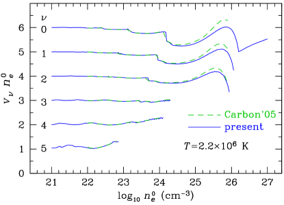
Figure 1: (Color online) Neutrality volumes $v_{\nu}$ normalized with the fiducial number density of free electrons $n_{e}^{0}$ (see text), as functions of $n_{e}^{0}$ for $T=2.2\times 10^{6}$ K for carbon ions with $\nu$ bound electrons ($\nu=0,1,\ldots,5$). The results from Ref. Potekhin et al. (2005) (dashed lines) are compared with the present improved results (solid lines).

The free electron density $n_{f}^{j\nu}(r)$ and the potential $V_{f}^{j\nu}(r)$ are determined self-consistently in the potential generated by the nucleus charge and a Boltzmann average of the $\nu$-electron wave-functions, solving for Kohn-Sham states in the local density approximation of the DFT, and assuming Fermi distribution of the free electrons at a given chemical potential $\mu_{e}$. The contributions from resonances are taken into account, as explained in Refs. Massacrier (1994); Potekhin et al. (2005). Together with $n_{f}^{j\nu}$ and $V_{f}^{j\nu}$, the ion sphere radii $R_{j\nu}$ and the corresponding neutrality volumes $v_{j\nu}=4\pi R_{j\nu}^{3}/3$ are obtained from the neutrality condition for each ion.

For a uniform free electron background, we would have $v_{j\nu}=v_{j\nu}^{0}=(Z_{j}-\nu)/n_{e}^{0}$, where $n_{e}^{0}(\mu_{e},T)$ is the “fiducial” electron density, which would correspond to the true electron density of the ideal Fermi gas of electrons at the given $\mu_{e}$ and $T$ values. When taking into account the interactions of the free electrons with the ions, $v_{j\nu}$ deviates from $v_{j\nu}^{0}$, as illustrated in Figs. 1 and 2 for carbon and oxygen plasmas, respectively. The drops of the curves at certain values of $n_{e}^{0}(\mu_{e},T)$, which are especially sharp at lower temperatures (see Fig. 2), are the consequence of pressure ionization of separate bound levels: when a $nl$ level of ion $\nu+1$ crosses the continuum limit and appears as a resonance in the neighboring ionization state $\nu$, the corresponding ion sphere shrinks to compensate this increase in the free electron density of states (note that $Z-\nu$ free electrons are still present in the volume $v_{j\nu}$). For a given level $nl$, pressure ionization occurs at electronic densities which roughly depend on the ionic charge as $(Z_{j}-\nu)^{4}$. If the number of bound states that remain in the ion sphere is not sufficient to accept $\nu$ electrons, that ion disappears: $\nu=5,6,7$ disappear with the $2p$ sub-shell, and $\nu=3,4$ with $2s$, see Figs. 1 and 2. We emphasize that, in contrast to average-atom models, separate ions have their own fate. Compared to Ref. Potekhin et al. (2005), we have extended the calculation of the free electron states to higher electron energies and to higher $\mu_{e}$. The consequences of these improvements for the neutrality volumes are seen in Fig. 1, where the dashed lines show our previous results and the solid lines correspond to our new calculations. The extension of $\mu_{e}$ to higher values allows us to capture the last dips of the neutrality volumes of naked nuclei ($\nu=0$) as functions of $n_{e}^{0}$, which appear at $n_{e}^{0}>10^{26}$ cm^-3 for both carbon and oxygen. These dips are due to the coupling of the hydrogenlike ($\nu=1$) bound states to the continuum, and are related to the pressure ionization of the K shell (where the curves $\nu=1$ in Figs. 1 and 2 terminate).

Pressure ionization of each atomic shell is accompanied by a spreading of the electronic level into a band, eventually passing into the continuum. We account for this effect by using occupation probabilities $w_{j\nu\alpha}=\prod_{(nl)\in\alpha}w_{j\nu nl}$, which are equal to the fraction of the band corresponding to the electron configuration $\alpha$ that remains below the continuum level at given $(T,\mu_{e})$ values (see Ref. Potekhin et al. (2005) for details).

In order to get a smooth pressure ionization and a smooth extension from calculated values of the neutrality volumes to higher densities, we replace $v_{j\nu}$ by $v_{j\nu}^{\ast}=v_{j\nu}w_{j\nu}+v_{j\nu}^{0}(1-w_{j\nu})$, where $w_{j\nu}$ is the occupation probability $w_{j\nu\alpha}$ calculated for the ground-state configuration $\alpha$ of the ion with $\nu$ electrons.

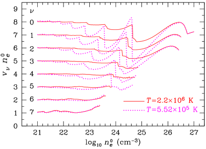
Figure 2: (Color online) Neutrality volumes $v_{\nu}$ normalized with $n_{e}^{0}$ (analogous to Fig. 1), as functions of $n_{e}^{0}$ for $T=2.2\times 10^{6}$ K (solid lines) and $T=5.52\times 10^{5}$ K (dotted lines) for oxygen ions with $\nu$ bound electrons ($\nu=0,1,\ldots,7$).

The separation of $H_{\nu}$ into parts (4) and (5) allows us to capture the plasma effects in one-electron energies and wave functions through Eqs. (4) and (6), while the $\nu$-electron structure – configuration energy mean shifts and $LS$ splitting – results from the contribution $W_{\nu}$. In Ref. Potekhin et al. (2005) we calculated this contribution to binding energies using a modified version of the “Superstructure” code Eissner and Nussbaumer (1969), as in Ref. Massacrier (1994). But our experience has revealed that the use of the atomic code is unnecessary for our purposes. This contribution is calculated once for the isolated ion and then combined with the one-electron energies $\epsilon_{j\nu nl}$ (see above) at any density. Indeed the dependence of this contribution on the plasma conditions is weak (of the second order in perturbation) compared to the dependence of the energies $\epsilon_{j\nu nl}$. In the present work we have updated the corrections due to $W_{\nu}$ by using the detailed atomic energy database of the Opacity Project (OP) (Ref. Seaton (2005) and references therein).

Having calculated energies $E_{j\nu\alpha}$ and occupation probabilities $w_{j\nu\alpha}$ at given values $(T,\mu_{e})$, we obtain the contribution of the internal degrees of freedom of all the ions to the free energy as

$$F_{\mathrm{int}}=-N_{i}k_{\mathrm{B}}T\sum_{j}\sum_{\nu=0}^{Z_{j}}x_{j\nu}\ln\mathcal{Z}_{j\nu},$$ (7)

where $\mathcal{Z}_{j\nu}=\sum_{\alpha}w_{j\nu\alpha}\,(2S+1)(2L+1)\,\exp(-E_{j\nu\alpha}/k_{\mathrm{B}}T)$ is the internal partition function of the ion $(j,\nu)$ in the plasma, and $x_{j\nu}\equiv N_{j\nu}/N_{i}$ its number fraction ($\sum_{j,\nu}x_{j\nu}=1$). Since we do not consider neutral atoms, the actual upper limit of $\nu$ summation is $Z_{j}-1$.

IV Thermodynamic equilibrium

We use a generalization of the free energy minimization method of Ref. Potekhin et al. (2005) to the case of multicomponent mixtures. The minimum of $F_{\mathrm{tot}}$ is sought at constant $V$, $T$, and $N_{j}$. The free parameters are the chemical potential $\mu_{e}$ and the ion fractions $x_{j\nu}$, subject to constraints

$$x_{j\nu}\geqslant 0,\quad\sum_{\nu=0}^{Z_{j}-1}x_{j\nu}=Y_{j},\quad N_{i}\sum_{j}\sum_{\nu=1}^{Z_{j}-1}x_{j\nu}v_{j\nu}=V,$$ (8)

where $Y_{j}$ are fixed chemical element abundances ($Y_{j}\geqslant 0$, $\sum_{j}Y_{j}=1$). The last condition in Eq. (8) reflects that $V$ is constant. We ensure this condition by using the Lagrange multiplier method. The other conditions in Eq. (8) are imposed explicitly in our minimization procedure by allowing the set of $\{x_{j\nu}\}$ to contain only the values for which these constraints are satisfied. Note that the charge neutrality condition is fulfilled automatically, because the volume $v_{j\nu}$ around every nucleus is neutral by construction. Some further details of the minimization algorithm can be found in Ref. Potekhin et al. (2005). For a mixture of chemical elements, we have in total $1+\sum_{j}(Z_{j}-1)$ independent parameters of minimization.

The minimization procedure provides the values of $F_{\mathrm{tot}}$ with a typical accuracy of four digits. Further improvement of the accuracy becomes problematic. The main sources of the numerical noise are the finite precision of calculation of the internal partition functions and neutrality volumes and the finite precision of the minimization procedure. The achieved accuracy is not sufficient for an accurate evaluation of thermodynamic functions, especially those that involve second and mixed derivatives of $F_{\mathrm{tot}}$ (specific heat $C_{V}$, logarithmic pressure derivatives with respect to density, $\chi_{\rho}$, and temperature, $\chi_{T}$, adiabatic temperature gradient, and so on). To overcome this difficulty, we use an additional filtering of the numerical noise after the minimization. The filtering procedure is modified relative to that in Ref. Potekhin et al. (2005). Specifically, for the results shown in the next section, we have performed calculations for a grid of points $(\rho,T)$ separated by $\Delta\log_{10}\rho=0.05$ and $\Delta\log_{10}T=0.1$, and at each point we have determined an improved value of $F_{\mathrm{tot}}$ using a bicubic 10-parameter polynomial fit to $F_{\mathrm{tot}}(\rho,T)$ on this grid. The fitting was done by $\chi^{2}$ minimization with weights decreasing with increasing distance between a given point $(\rho,T)$ and the grid point $(\rho^{\prime},T^{\prime})$ in the $\log_{10}\rho$–$\log_{10}T$ plane as $[1+(\log_{10}(\rho^{\prime}/\rho)/\Delta\log_{10}\rho)^{2}+(\log_{10}(T^{\prime}/T)/\Delta\log_{10}T)^{2}]^{-1}$. This improved method of primary filtering of numerical noise allows us to avoid the additional secondary smoothing of thermodynamic functions that was employed in Ref. Potekhin et al. (2005).

V Results

V.1 Ionization equilibrium

The minimization of the total free energy immediately gives a solution to ionization equilibrium. Examples of partial fractions of ions as functions of $T$ at constant $\rho$, or of $\rho$ at constant $T$, are shown in Figs. 3–6, as well as in panels (b) of Figs. 7 and 8 in Sect. V.2. Figure 3 shows current results (solid lines) in a pure carbon plasma for the partial fractions of ions with different numbers of electrons (marked by the numbers near the respective curves) and for the mean effective charge (marked by the symbol $\langle Z\rangle$ and scaled to the right vertical axis) at (a) $\rho=0.2$ g cm^-3 and (b) $\rho=10$ g cm^-3 . This effective charge is calculated by taking into account the partial delocalization of the outer-shell electrons in the pressure ionization region as $\langle Z\rangle=\sum_{j\nu}(Z_{j}-\nu+1-w_{j\nu})\,x_{j\nu}$. The ions recombine with decreasing temperature at both densities, but at the high density $\rho=10$ g cm^-3 there is no room for the existence in carbon of bound states other than $1s$ (as can be inferred from Fig. 1, though for a fixed temperature: $\rho=10$ g cm^-3 corresponds to $n_{e}\simeq~{}2$ – $3\times 10^{24}$ cm^-3.) Hence recombination can not proceed past the He-like ($\nu=2$) stage.

The dashed lines in the figure correspond to a simplified approach, where the neutrality volumes $v_{j\nu}$ and internal partition functions $\mathcal{Z}_{j\nu}$ are calculated assuming the uniform electron density $n_{e}=n_{e}^{0}$. In this simple approximation we can obtain results in a wider range of $T$ than in the accurate calculation. This approximation works well at relatively low densities, as proved by the good agreement of the dashed and solid curves in Fig. 3(a). With increasing density, the coupling of the bound and continuum states becomes significant. More accurate calculation becomes necessary, as can be seen in Fig. 3(b), especially at low temperatures where the difference in the ion sphere between a uniform free electron density and the density constructed from quantum continuum states will be more pronounced.

We also report on Fig. 3 the mean ion charge as obtained from FLYCHK (dash-dotted lines), a suite of codes based on simplified atomic models aimed at providing fast collisional-radiative models and spectra Chung et al. (2005). FLYCHK gives generally a lower mean effective charge, especially at temperature-density conditions where several ionization stages are present. This is probably due to its treatment of density effects through a simplified approach. The experimental data points of Gregori et al. (2008) for $\langle Z\rangle$ are plotted in Fig. 3(a) as circles. They agree with our results at this density, especially if one considers the experimental uncertainties of $\pm 20$ eV for the temperature and $\pm 0.25$ for $\langle Z\rangle$ . Experiments at higher densities would certainly be very valuable.

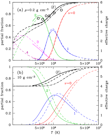
Figure 3: (Color online) Number fractions of different carbon ions (left vertical axis, marked by the numbers of bound electrons $\nu$ near the curves) and mean effective charge $\langle Z\rangle$ (right vertical axis) in a pure plasma versus temperature at (a) $\rho=0.2$ g cm^-3 and (b) $\rho=10$ g cm^-3. Solid lines: accurate results; dashed lines: approximation where partition functions $\mathcal{Z}_{j\nu}$ and neutrality volumes $v_{j\nu}$ are calculated assuming a uniform free electron density. Dash-dotted line: results for $\langle Z\rangle$ from FLYCHK Chung et al. (2005). In panel (a) the circles are the experimental results from Gregori et al. (2008) for $\rho=0.2$ g cm^-3.

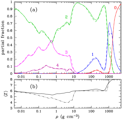
Figure 4: (Color online) (a) Number fractions of ions for a pure oxygen plasma (solid lines) at $T=6\times 10^{5}$ K as a function of the density $\rho$. Numbers of bound electrons $\nu$ for each ion are marked near the curves. Dashed lines are twice the ionization fractions $x_{j\nu}$ for oxygen in a plasma mixture composed of equal numbers of C and O nuclei at the same temperature. (b) Mean effective charge $\langle Z\rangle$ for the pure oxygen plasma (solid line). The dot-dashed line is the result from FLYCHK under the same conditions.

The effects of pressure ionization are most appreciable in Fig. 4, where ion population fractions (a) and the mean effective charge (b) for a pure oxygen plasma (solid lines) are plotted versus density at $T=6\times 10^{5}$ K. The results of FLYCHK for $\langle Z\rangle$ are also reported on Fig. 4(b) (dot-dashed line). Recombination with increasing density is modulated at the lowest densities ($\rho\lesssim 0.5$ g cm^-3) by the successive pressure ionizations of the Li-like ($\nu=3$) ion shells (see Fig. 2: $\rho=0.5$ g cm^-3 corresponds to $n_{e}\simeq 10^{23}$ cm^-3 for $\langle Z\rangle=5.5$). The temperature is sufficient to populate excited states of that ion but not of He-like ions, so that only the Li-like ion partition function is affected (the $1s^{2}~{}2s$–$1s^{2}~{}3s$ energy difference is $9\times 10^{5}$ K, while the $1s^{2}$–$1s~{}2s$ one is $6.5\times 10^{6}$ K). Between $\rho\simeq 0.5$ g cm^-3 and $20$ g cm^-3, Li-like ions gradually disappear with the $n=2$ shell to the benefit of He-like ions. On the contrary (see Fig. 4(b)), FLYCHK still allows recombination into the Be-like ion ($\nu=4$) until $\rho\simeq 8$ g cm^-3 where it is sharply pressure ionized, just before Li-like ions. Oxygen remains at higher densities in the He-like stage up to $\rho\simeq 10^{3}$ g cm^-3 where the last $1s$ shells for He-like and H-like ions are moved into the continuum. In this density range our results show a more complex behaviour due to several effects: the free electrons become degenerate, the ionization occurs on a large density range due to band broadening, and the influence of neutrality volumes is strong.

Dashed lines in Fig. 4(a) show the ionization fractions of oxygen in a mixture of equal numbers of C and O nuclei. The fractions $x_{j\nu}$ have been multiplied by two to be compared with the pure oxygen plasma case. The behavior of the ionization equilibrium of oxygen is quite similar in the two cases, the biggest difference occurring in the pressure ionization zone around $\rho\simeq 10^{3}$ g cm^-3. In Fig. 5 we show the temperature dependence of the partial ion fractions for the two chemical elements C (dotted lines) and O (solid lines) in the same mixture at $\rho=1$ g cm^-3. At this density, the curves for the fraction of $\nu$-ions for carbon are roughly shifted to lower temperatures when compared to the oxygen ones by the ratio of the ionization energies $(Z_{C}-\nu)^{2}/(Z_{O}-\nu)^{2}$.

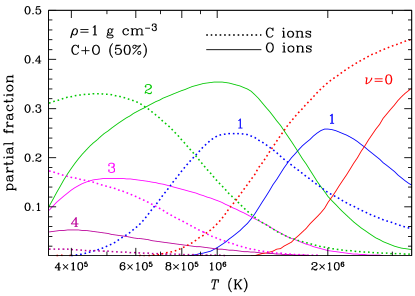
Figure 5: (Color online) Number fractions of different carbon (dotted lines) and oxygen (solid lines) ions in the mixture of equal number of ions of each chemical element at $\rho=1$ g cm^-3 as functions of $T$.

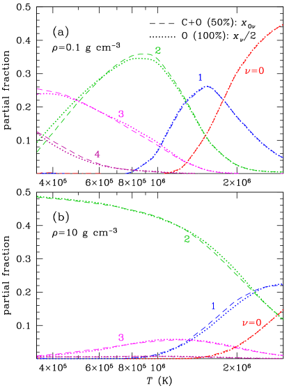
Figure 6: (Color online) Number fractions of different oxygen ions as functions of $T$ in the mixture of equal number of ions of each chemical element C and O at (a) $\rho=0.1$ g cm^-3  and (b) $\rho=10$ g cm^-3. Dashed lines show the result of direct free energy minimization for the mixture, and dotted lines show the result of an approximation based on the solution of the ionization equilibrium problem for pure C and O plasmas (see text).

Comparing Fig. 5 and analogous figures for mixtures and pure substances, we notice that the temperature and density dependences of partial ion fractions in mixtures of different elements are similar to those in pure substances, scaled by the element abundances $Y_{j}$. Two examples are presented in Fig. 6. Here, the dashed lines show partial fractions $x_{j\nu}$ of oxygen ions with $\nu$ bound electrons in a mixture where half the ions are oxygen ions and half are carbon ions, at (a) $\rho=0.1$ g cm^-3 and (b) $\rho=10$ g cm^-3, as function of $T$, while the dotted lines show fractions of the same ions, multiplied by 0.5, in a pure oxygen plasma. The close agreement between these curves, which has been tested at several densities (see, e.g., Fig. 4(a)) or compositions, prompted us to suggest the following method for an approximate solution of the ionization equilibrium problem and a construction of the EOS for plasma mixtures of different elements (at least in the temperature range considered in the present study):

• calculate the fractional numbers of different ions $x_{j\nu}$ for pure substances at the same $n_{e}$ and $T$ (let us denote their values $x_{j\nu}^{0}$);

• multiply them by $Y_{j}$ and keep them fixed: $x_{j\nu}=x_{j\nu}^{0}Y_{j}$;

• adjust the electron chemical potential $\mu_{e}$ so as to fulfill the last condition in Eq. (8).

The advantage of this method for a mixture of $J$ chemical elements is that, instead of minimizing $F_{\mathrm{tot}}$ in a space of $1+\sum_{j=1}^{J}(Z_{j}-1)$ independent parameters, one needs to perform $J$ minimizations in a space of $Z_{j}$ parameters each, and then to adjust $\mu_{e}$. As a rule, these $J$ partial minimizations go much faster than the single minimization in the space of all parameters, thus saving the computer cost of the procedure. For example, it is much easier to find the minima of $F_{\mathrm{tot}}$ for carbon (6 parameters) and for oxygen (8 parameters) separately, than to find a minimum for their mixture (13 parameters). Moreover, having found the number fractions of ions for pure substances once, one can calculate thermodynamic functions of mixtures with any fractions of chemical elements $Y_{j}$ without repeating the whole minimization procedure. Note however that carbon and oxygen are chemical species that are not very different, so that one should proceed with caution before applying this simplified approach to other mixtures without further studies.

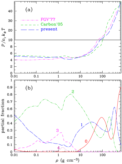
Figure 7: (Color online) (a) Normalized pressure $PV/N_{i}k_{\mathrm{B}}T$ for pure carbon along the isotherm $T=5\times 10^{5}$ K. The present results (long-dashed line) are compared with the results from Ref. Fontaine et al. (1977) (dot-dashed line) and Ref. Potekhin et al. (2005) (short-dashed line). Note the different scale in the figure above and below the middle horizontal line. (b) Number fractions of different carbon ions (present results) for the same temperature.

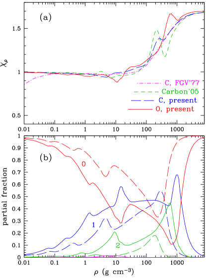
Figure 8: (Color online) (a) Logarithmic pressure derivative $\chi_{\rho}=\partial\ln P/\partial\ln\rho$ along the isotherm $T=3.16\times 10^{6}$ K. The present data for carbon (long-dashed line) are compared with the results from Ref. Fontaine et al. (1977) (dot-dashed line) and Ref. Potekhin et al. (2005) (short-dashed line). The solid line shows the isotherm of $\chi_{\rho}$ for oxygen. (b) Present results for the number fractions of carbon ions (dashed lines) and oxygen ions (solid lines) at the same temperature.

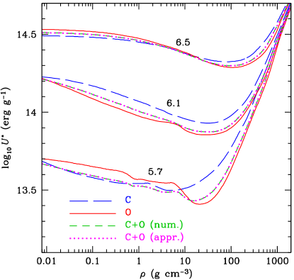
Figure 9: (Color online) Specific internal energy logarithms (in cgs units) for various isotherms: $T=5\times 10^{5}$ K, $1.26\times 10^{6}$ K, and $3.16\times 10^{6}$ K (the curves are marked by $\log_{10}T$ values) for oxygen (solid lines), carbon (long-dashed lines), and the mixture of equal number of ions of each chemical element (short-dashed and dotted lines). In the latter case short-dashed lines show the result of direct free energy minimization for the mixture, while dotted lines show the result of an approximation based on the solution of the ionization equilibrium problem for pure C and O plasmas (the difference between them is almost unnoticeable; see text).

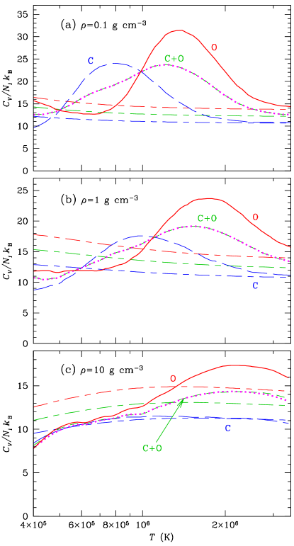
Figure 10: (Color online) Normalized specific heat per ion for the isochores (a) $\rho=0.1$ g cm^-3 , (b) $\rho=1$ g cm^-3 , and (c) $\rho=10$ g cm^-3 for carbon (long-dashed line), oxygen (solid line), and mixture of equal number of ions of each chemical element (short-dashed and dotted lines). In the latter case, the short-dashed line shows the result of direct free energy minimization for the mixture, while the dotted line shows the result of an approximation based on the solution of the ionization equilibrium problem for pure C and O plasmas. For comparison, alternating short and long dashes show analogous isochores for the fully ionized plasma model.

V.2 Thermodynamic functions

To illustrate our results for the EOS and compare them with the results of Ref. Potekhin et al. (2005), we show in Fig. 7(a) an isotherm for the pressure $P(\rho)$ for carbon at $T=5\times 10^{5}$ K. Our present result is shown by the long-dashed line, our previous result Potekhin et al. (2005) by short dashes, and the dot-dashed line shows the result obtained with the FGV EOS Fontaine et al. (1977) based on a Thomas-Fermi model at $\rho\gtrsim 3$ g cm^-3. In order to make the differences visible in the figure, we have normalized the pressure by its value for an ideal Boltzmann gas of ions, $N_{i}k_{\mathrm{B}}T/V$. The vertical scale is smaller for the upper part of the figure, to take into account the rapidly increasing pressure contribution of degenerate electrons. The differences between our and FGV results have become smaller for $\rho\gtrsim 10$ g cm^-3 than in Ref. Potekhin et al. (2005), and the additional features have become less spectacular. This change is mainly caused by the improved treatment of the electron continuum in the present work (see Sec. II).

However, the additional features still persist near the densities where electron shells become pressure ionized, as expected. For instance it can be seen from the ionization fractions as given in Fig. 7(b) for the same isotherm that the feature in the pressure just above $\rho=1$ g cm^-3 is linked to the disappearance of the Li-like carbon ion. These features are clearly revealed in the logarithmic derivative of the pressure, $\chi_{\rho}=(\partial\ln P/\partial\ln\rho)_{T}$, shown in Fig. 8(a). In this panel, the dot-dashed, short-dashed, and long-dashed lines correspond to the same three models for carbon plasma as in Fig. 7(a). In addition, the solid line shows $\chi_{\rho}$ for the oxygen plasma at the same temperature. When analyzed with the help of the ionization fractions as plotted in Fig. 8(b) the features for carbon around $\rho\simeq 5$ g cm^-3 and $3\times 10^{2}$ g cm^-3 appear to be linked to the pressure ionization in H-like ions of the $n=2$ and $n=1$ shells respectively; those for oxygen around $\rho\simeq 10$ g cm^-3 and $6\times 10^{2}$ g cm^-3 are linked to the same shells with a supplementary contribution from the He-like ions. In the latter case, the features due to pressure ionization are more pronounced because of the higher binding energies compared to carbon, and they are shifted to higher densities because of the higher net charge and respectively smaller neutrality volumes of ions (this shift can be roughly estimated as the ratio of the volumes of hydrogen-like carbon and oxygen ions, $\sim(Z_{O}/Z_{C})^{3}=64/27$). Note also that the pressure ionization of a given (sub-)shell leaves an imprint on thermodynamics functions at different densities depending on which ionization stage is dominant. For instance the features due to the $n=2$ shell in carbon appear at $\rho\simeq 1$ g cm^-3  or $5$ g cm^-3 depending on whether Li-like or H-like ions are concerned (compare Fig. 7 and Fig. 8).

Figure 9 shows three isotherms for the internal energy per unit mass for carbon (long-dashed lines), oxygen (solid lines), and the mixture containing equal numbers of C and O nuclei (short-dashed and dotted lines). The energy per unit mass $U^{*}=U/(N_{i}\sum_{j}m_{j}Y_{j})+U_{0}^{*}$ is measured from the ground state energy of nonionized atoms, which corresponds to a shift with respect to the electron continuum level equal to $U_{0}^{*}=\sum_{j}Y_{j}U_{0,j}^{*}$, where $U_{0,j}^{*}=8.28\times 10^{13}$ erg g^-1 for carbon and $U_{0,j}^{*}=1.23\times 10^{14}$ erg g^-1 for oxygen. For the mixture, the short-dashed lines portray the results of the numerical minimization of the complete free energy $F_{\mathrm{tot}}$, while the dotted lines illustrate the results of the approximate method described in Sec. V.1. The near coincidence of the dotted and short-dashed lines, indistinguishable at the scale of the figure, confirms the accuracy of the approximate method in that case.

As an example of a second-order thermodynamic function calculated with our model, Fig. 10 presents isochores for the heat capacity at (a) $\rho=0.1$ g cm^-3 , (b) $\rho=1$ g cm^-3 , and (c) $\rho=10$ g cm^-3  for carbon (long-dashed line), oxygen (solid line), and the carbon-oxygen mixture with $Y_{j}=0.5$. For the mixture, the short-dashed lines portray the results of the numerical minimization of the complete free energy $F_{\mathrm{tot}}$, while the dotted lines illustrate the results of the approximate method described in Sec. V.1. As well as in Fig. 9, the short-dashed and dotted lines nearly coincide. For comparison, lines drawn with alternating short and long dashes show the results obtained for the fully ionized plasma model. The presence of bound states yields big bumps on the curves. Comparison with Figs. 3 and 6 (for $0.1-0.2$ g cm^-3 and $10$ g cm^-3) and with Fig. 5 (for $1$ g cm^-3) reveals that these bumps are associated with the thermal ionization of heliumlike ions into hydrogenlike ones and then into nuclei. At higher temperatures, the results for fully ionized plasmas are recovered, as it should be due to the complete ionization of C and O at such high temperatures, in agreement with the Saha equation.

VI Conclusions

We have further improved our model Potekhin et al. (2005) for the calculation of the EOS for dense, partially ionized plasmas, based on the free energy minimization method, suitable to handle pressure ionization regimes. The free energy model is constructed in the framework of the chemical picture of plasmas and includes a detailed, self-consistent treatment of the quantum states of partially ionized atoms in the plasma environment as well as a quantum treatment of the continuum electrons. The improvements with respect to our former pure carbon calculations include implementing updated fitting formulae Potekhin et al. (2009); Potekhin and Chabrier (2010) for the long-range Coulomb contribution to the free energy, the use of the OP database for energies of bound state configurations Seaton (2005), an increased range of density and the extension to mixtures of different chemical elements.

We have extended the calculations from pure carbon to arbitrary carbon-oxygen mixtures. We have also suggested an efficient, approximate but accurate method of EOS calculation in the case of mixtures of different chemical elements, based on the detailed information about the various ionic state fractions for the pure species.

The present EOS results can be used in studies of carbon-oxygen plasmas in the domain of so-called warm dense matter as well as in astrophysical calculations of stellar structure and evolution. The possible astrophysical applications include oxygen and carbon plasmas and carbon-oxygen mixtures in various types of stars, for example the interiors of carbon-oxygen white dwarfs. However, in order to apply it also to the outer parts of the white dwarf envelopes, it is desirable to extend the results to lower temperatures. We are planning to perform such extensions in the future work.