The ACS Survey of Galactic Globular Clusters. XII. Photometric Binaries along the Main-Sequence

Context. The fraction of binary stars is an important ingredient to interpret globular cluster dynamical evolution and their stellar population.
Aims. We investigate the properties of main-sequence binaries measured in a uniform photometric sample of 59 Galactic globular clusters that were observed by HST WFC/ACS as a part of the Globular Cluster Treasury project.
Methods. We measured the fraction of binaries and the distribution of mass-ratio as a function of radial location within the cluster, from the central core to beyond the half-mass radius. We studied the radial distribution of binary stars, and the distribution of stellar mass ratios. We investigated monovariate relations between the fraction of binaries and the main parameters of their host clusters.
Results. We found that in nearly all the clusters, the total fraction of binaries is significantly smaller than the fraction of binaries in the field, with a few exceptions only. Binary stars are significantly more centrally concentrated than single MS stars in most of the clusters studied in this paper. The distribution of the mass ratio is generally flat (for mass-ratio parameter q$>$0.5). We found a significant anti-correlation between the binary fraction in a cluster and its absolute luminosity (mass). Some, less significant correlation with the collisional parameter, the central stellar density, and the central velocity dispersion are present. There is no statistically significant relation between the binary fraction and other cluster parameters. We confirm the correlation between the binary fraction and the fraction of blue stragglers in the cluster.

1 Introduction

The knowledge of the binary frequency in Globular Clusters (GCs) is of fundamental importance in many astrophysical studies. Binaries play an important role in the cluster dynamical evolution, as they represent an important source of heating. They are also important for the interpretation of the stellar populations in GCs. A correct determination of the stellar mass and luminosity functions in GCs requires accurate measure of the fraction of binaries. Stellar evolution in a binary system can be different from isolated stars in the field. Exotic stellar objects, like Blue Stragglers (BSSs), cataclysmic variables, millisecond pulsars and low mass X-ray binaries represent late evolutionary stages of close binary systems. The determination of the fraction of binaries plays a fundamental role towards the understanding of the origin and evolution of these peculiar objects.

There are three main techniques used in literature to measure the fraction of binaries in GCs (Hut et al. 1992). The first one identifies binaries by measuring their radial velocity variability (e. g. Latham 1996). This method relies on the detection of each individual binary system but, due to actual limits in sensitivity of spectroscopy, these studies are possible only for the brightest GC stars. Moreover, this technique is sensitive to binaries with short orbital periods, and the estimated fraction of binaries depends on the eccentricity distribution. The second approach is based on the search for photometric variables (e. g. Mateo 1996). As in the previous case, it is possible to infer specific properties of each binary system (like the measure of orbital period, mass ratio, orbital inclination). Unfortunately, this method is biased towards binaries with short periods and large orbital inclination. The estimated fraction of binaries depends on the assumed distribution of orbital periods, eccentricity and mass ratio. Both of these techniques have a low discovery efficiency and are very expensive in terms of telescope time because of the necessity to repeat measures in different epochs.

A third method, based on the analysis of the number of stars located on the red side of the MS fiducial line, may represent a more efficient approach to measure the fraction of binaries in a cluster for several reasons:

• The availability of a large number (thousands) of stars makes it a statistically robust method;

• It is efficient in terms of observational time: two filters are enough for detecting binaries, and repeated measurements are not needed.

• It is sensitive to binaries with any orbital period and inclination.

This latter approach has been used by many authors (e. g. Aparicio et al. 1990, 1991, Romani & Weinberg 1991, Bolte 1992, Rubenstein & Baylin 1997, Bellazzini et al. 2002, Clark, Sandquist & Bolte 2004, Richer et al. 2004, Zhao & Baylin 2005, Sollima et al. 2007, 2009, Bedin et al. 2008, Milone et al. 2009, 2010, 2011) to study the populations of binaries in individual stellar clusters. The relatively small number of clusters that have been analyzed is a consequence of the intrinsic difficulties of the method:

• High photometric quality is required and high resolution is necessary to minimize the fraction of blends in the central regions of GCs;

• Differential reddening (often present) spreads the MS and makes it more difficult to distinguish the binary sequence from the single-star MS population;

• An accurate analysis of photometric errors as well as a correct estimate of field contamination are necessary to distinguish real binaries from bad photometry stars and field objects.

The first study of binaries in a large sample of GCs comes from Sollima et al. (2007), who investigated the global properties of binaries in 13 low-density GCs. These authors found that the total fraction of binaries ranges from 0.1 to 0.5 in the core depending on the cluster, thus confirming the deficiency of binaries in GCs compared to the field where more than half of stars are in binary systems (Mayor et al. 1992, Dunquennoy & Mayor 1991, Fischer & Marcy 1992, Halbwachs et al. 2003, Rastegaev et al. 2010, Raghavan et al. 2010). At variance with the high fraction of binaries in field sdB stars (Masted et al. 2001, Napiwotzki et al. 2004), a lack of close binaries among GC hot horizontal branch stars (the cluster counterpart of field sdBs) has been confirmed by Moni Bidin et al. (2006, 2009).

Sollima et al. (2010) extended the study of binaries to five high-latitude open clusters with ages between $\sim$0.3-4.3 Gyr and found that the fraction of binaries are generally larger than in GCs and range between $\sim$0.3 and 0.7 in the core. Very high binary fractions have been observed also in some young star clusters and for pre-main sequence T-Tauri stars, where the total binary fraction might be as high as 0.9 (e. g. Prosser et al. 1994, Petr et al. 1998, McCaughrean 2001, Duchêne 1999).

These findings suggest that the star formation condition, as well as the environment, could play a fundamental role on the evolution of binary systems. The binary populations in star clusters has been investigated in detail, mainly through Monte-Carlo and Fokker-Plank simulations (e. g. Giersz & Spurzem 2000, Fregeau et al. 2003, Ivanova et al. 2005), N-body (e. g. Shara & Hurley 2002, Trenti, Heggie, & Hut 2007, Hurley, Aarseth, & Shara (2007), Fregeau et al. 2009, Marks, Kroupa, & Oh 2011) and fully analytical computations (Sollima 2008).

While the evolution of binaries stimulated by interactions with cluster stars could play the major role, there are many processes that also influence the binary population in stellar systems. For instance binary systems can form by tidal-capture (e. g. Hut et al. 1992, Kroupa 1995a). Destruction of binaries may occur via coalescence of components through encounters or tidal dissipation between the components (Hills 1984, Kroupa 1995b, Hurley & Shara 2003). Stellar evolutionary processes can significantly effect the property of binaries and binary-binary interaction can led to collisions and mergers (e. g. Fregeau et al. 2004). The comparison of simulation results with observed binary fraction is hence a powerful tool to shed light on both the cluster and the binaries evolution.

In this paper, we report the observational results of our search for photometric binaries among GCs present in the HST Globular Cluster Treasury catalog (Sarajedini et al. 2007, Anderson et al. 2008), which is based on HST ACS/WFC data We exploited both the homogeneity of this dataset, and the high photometric accuracy of the measures to derive the fraction of binaries in the densest regions of 59 GCs. We deserve to future works any attempt to interpret the empirical findings presented in this paper.

2 Observations and data reduction

Most of the data used in this paper come from the HST ACS/WFC images taken for GO 10775 (PI Sarajedini), an HST Treasury project, where a total of 66 GCs were observed through the F606W and F814W filters. For 65 of them, the database consists in four or five F606W and F814W deep exposures plus a short exposure in each band. The pipeline used for the data reduction allowed us to obtain precise photometry from nearly the tip of the red giant branch (RGB) to several magnitudes below the main sequence turn-off (MSTO), typically reaching $\sim$0.2 ${\it m}_{\odot}$.

The GO 10775 data set as well as the methods used for its photometric reduction have been presented and described in papers II and IV of this series (Sarajedini et al. 2007 and Anderson et al. 2008).

The uniform and deep photometry offers a database with unprecedented quality that made possible a large number of studies (see e. g. Sarajedini et al. 2010 and references therein).

In this paper we study the main sequence binary population in a subset of 59 GCs. We excluded three clusters (Lynga 7, NGC 6304, and NGC 6717) that are strongly contaminated by field stars and for which there exist no archive HST data which could allow us to obtain reliable proper motions and separate them from cluster members. We also excluded Palomar 2 because of its high differential reddening, and NGC 5139 ($\omega$ Centauri), and NGC 6715 because of the multiple main sequences (Siegel et al. 2007, Bellini et al. 2010 and references therein). The triple MS of NGC 2808 made the binary-population extremely complicated and we presented it in a separate paper (Milone et al. 2011a).

In addition, we also used archive HST WFPC2, WFC3 and ACS/WFC images from other programs to obtain proper motions, when images overlapping the GO10775 images were available. Table 1 summarizes the archive data used in the present paper.

The recipes of Anderson et al.  (2008) have been used to reduce the archive ACS/WFC data. The WFPC2 data are analyzed by using the programs and the techniques described in Anderson & King (1999, 2000, 2003). We measured star positions and fluxes on the WFC3 images with a software mostly based on img2xym_WFI (Anderson et al. 2006). Details on this program will be given in a stand-alone paper. Star positions and fluxes have been corrected for geometric distortion and pixel-area using the solutions provided by Bellini & Bedin (2009).

ID	DATE	N$\times$EXPTIME	FILT	INSTRUMENT	PROGRAM	PI
ARP 2	May 11 1997	1$\times$260s$+$5$\times$300s	F814W	WFPC2	6701	Ibata, R.
	May 11 1997	5$\times$300s$+$1$\times$350s	F606W	WFPC2	6701	Ibata, R.
NGC 104	Sep 30 2002 - Oct 11 2002	1$\times$10s$+$6$\times$100s$+$3$\times$115s	F435W	ACS/WFC	9281	Grindlay, G.
	Jul 07 2002	6$\times$60s$+$1$\times$150s	F475W	ACS/WFC	9443	King, I. R.
	Jul 07 2002	20$\times$60s	F475W	ACS/WFC	9028	Meurer, J.
NGC 362	Dec 04 2003	4$\times$340s	F435W	ACS/WFC	10005	Lewin, W.
	Dec 04 2003	2$\times$110s$+$2$\times$120s	F625W	ACS/WFC	10005	Lewin, W.
	Sep 30 2005	3$\times$70s$+$20$\times$340s	F435W	ACS/WFC	10615	Anderson, S.
NGC 5286	Jul 07 1997	3$\times$140s$+$1$\times$100s	F555W	WFPC2	6779	Gebhardt, K.
	Jul 07 1997	3$\times$140s$+$1	F814W	WFPC2	6779	Gebhardt, K.
NGC 5927	May 08 1994	6$\times$50s$+$8$\times$600s	F555W	WFPC2	5366	Zinn, R.
	May 08 1994	6$\times$70s$+$8$\times$800s	F814W	WFPC2	5366	Zinn, R.
	Aug 06 2002	30s+500s	F606W	ACS/WFC	9453	Brown, T.
	Aug 06 2002	15s+340s	F814W	ACS/WFC	9453	Brown, T.
	Aug 28 2010	50s$+$2$\times$455s	F814W	UVIS/WFC3	11664	Brown, T.
	Aug 28 2010	50s$+$2$\times$665s	F555W	UVIS/WFC3	11664	Brown, T.
NGC 6121	Jun 19 2003	15$\times$360s	F775W	ACS/WFC	9578	Rhodes, J.
NGC 6218	Jun 14 2004	4$\times$340s	F435W	ACS/WFC	10005	Lewin, W.
	Jun 14 2004	2$\times$40s$+$2$\times$60s	F625W	ACS/WFC	10005	Lewin, W.
NGC 6352	Mar 29 1995	7$\times$160s	F555W	WFPC2	5366	Zinn, R.
	Mar 29 1995	6$\times$260s	F814W	WFPC2	5366	Zinn, R.
NGC 6388	Jun 30 - Jul 03 2010	6$\times$880s	F390W	UVIS/WFC3	11739	Piotto, G.
NGC 6397	Aug 01 2004 - Jun 28 2005	5$\times$13s$+$5$\times$340s	F435W	ACS/WFC	10257	Anderson, J.
NGC 6441	Aug 04-08 2010	6$\times$880s	F390W	UVIS/WFC3	11739	Piotto, G.
NGC 6496	Apr 01 1999	2$\times$1100s+4$\times$1300s	F606W	WFPC2	6572	Paresce, F.
	Apr 01 1999	2$\times$1100s+4$\times$1300s	F814W	WFPC2	6572	Paresce, F.
NGC 6535	Aug 04 1997	8$\times$140s	F555W	WFPC2	6625	Buonanno, R.
	Aug 04 1997	9$\times$160s	F814W	WFPC2	6625	Buonanno, R.
NGC 6624	Oct 15 1994	6$\times$50s$+$8$\times$600s	F814W	WFPC2	5366	Zinn, R.
NGC 6637	Mar 31 1995	6$\times$60s$+$8$\times$700s	F814W	WFPC2	5366	Zinn, R.
NGC 6652	Set 05 1997	12$\times$160s	F814W	WFPC2	6517	Chaboyer, B.
NGC 6656	Feb 22 1999 - Jun 15 1999	192$\times$260s	F814W	WFPC2	7615	Sahu, K.
	Feb 22 1999 - Jun 15 1999	72$\times$260s	F606W	WFPC2	7615	Sahu, K.
NGC 6681	May 09 2009	32$\times$300s	F450W	WFPC2	11988	Chaboyer, B
NGC 6838	May 21 2000	2$\times$100s	F439W	WFPC2	8118	Piotto, G.
	May 21 2000	2$\times$30s	F555W	WFPC2	8118	Piotto, G.
TERZAN 7	Mar 18 1997	1$\times$260s$+$5$\times$300s	F814W	WFPC2	6701	Ibata, R.
	Mar 18 1997	5$\times$300s$+$1$\times$350s	F606W	WFPC2	6701	Ibata, R.

Table 1: Description of the HST additional archive data sets used in this paper, other than those from GO-10775.

2.1 Selection of the star sample

Binaries that are able to survive in the dense environment of a GC are so close that even the Hubble Space Telescope HST is not able to resolve the single components. For this reason, light coming from each star will combine, and the binary system will appear as a single point-like source. In this paper we will take advantage from this fact to search for binaries by carefully studying the region in the CMD where their combined light puts them.

If we consider the two components of a binary system and indicate with $m_{1}$, $m_{2}$, $F_{1}$, and $F_{2}$ their magnitudes and fluxes, the binary will appear as a single object with a magnitude:

$m_{\rm bin}=m_{1}-2.5\leavevmode\nobreak\ log(1+\frac{F_{2}}{F_{1}})$.

In the case of a binary formed by two MS stars (MS-MS binary) the fluxes are related to the two stellar masses ($\mathcal{M}_{1}$, $\mathcal{M}_{2}$), and its luminosity depends on the mass ratio $q=\mathcal{M}_{2}/\mathcal{M}_{1}$ (in the following we will assume $\mathcal{M}_{2}<\mathcal{M}_{1}$, $q<1$). The equal-mass binaries form a sequence that is almost parallel to the MS, $\sim$0.75 magnitudes brighter. When the masses of the two components are different, the binary will appear redder and brighter than the primary and populate a CMD region on the red side of the MS ridge line (MSRL) but below the equal-mass binary line.

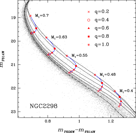
Figure 1: Model MS-MS binary sequences with different mass ratios for NGC 2298. The dashed-dotted line is the MSRL while, continuous black lines indicate the sequences of constant q and blue lines mark sequences of constant ${\mathcal{M}}_{1}$.

In Fig. 1 we used our empirical MSRL and the mass-luminosity relations of Dotter et al. (2007) to generate sequences of MS-MS binary systems with different mass ratios.

An obvious consequence of this analysis is that our capability in detecting binaries mainly depends on the photometric quality of the data. Distinguishing the binary populations in clusters requires high-resolution images and high-precision photometry. Not all stars in clusters can be measured equally well. Crowding, saturation, and image artifacts such as diffraction spikes, bleeding columns, hot pixels, and cosmic rays can prevent certain stars from being measured well. The first challenge to this project will be to identify which stars can be measured well and which are hopeless.

In addition to the basic stellar positions and photometry, the software described in Anderson et al. (2008) calculates several useful parameters that will help us reach this goal. The following parameters are provided for every star:

• The rms of the positions measured in different exposures and transformed into a common reference frame ( ${\it rms}_{\rm X}$ and ${\it rms_{\rm Y}}$)

• The average residuals of the PSF fit for each star (${\it q}_{\rm F606W}$ and ${\it q}_{\rm F814W}$ )

• The total amount of flux in the 0.5 arcsec aperture from neighboring stars relative to the star’s own flux (${\it o}_{\rm F606W}$ and ${\it o}_{\rm F814W}$).

True binary stars will be so close to each other as to be indistinguishable from single stars in our images, so the binarity has no impact on the above diagnostics. Therefore, it is safe to use the above diagnostics to indicate which stars are likely measured well and which ones are likely contaminated. As an example, in the six panels of Fig.2, we show these parameters as a function of the instrumental ${\it m}_{\rm F606W}$ and ${\it m}_{\rm F814W}$ magnitudes, and illustrate the criteria that we have used to select the sample of stars with the best photometry for NGC 2298.

We note a clear trend in the quality fit and the rms parameters as a function of the magnitude. At all magnitudes, there are outliers that are likely sources with poorer photometry and that need to be removed before any analysis. Because of this, we adopted the following procedure to select the best measured stars.

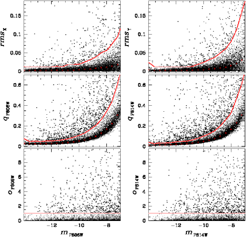
Figure 2: Diagnostic parameters that we have used to select the sample of NGC 2298 stars with high-quality photometry. The parameters are plotted as a function of the instrumental ${\it m}_{\rm F606W}$ and ${\it m}_{\rm F814W}$ magnitudes. Red circles indicate the median ${\it rms}_{\rm X,Y}$, and ${\it q}_{\rm F606W,F814W}$ per intervals of 0.4 magnitude. Red lines separate the well measured stars (thin points) from those that are more likely to have poorer photometry (thick points). See text for details.

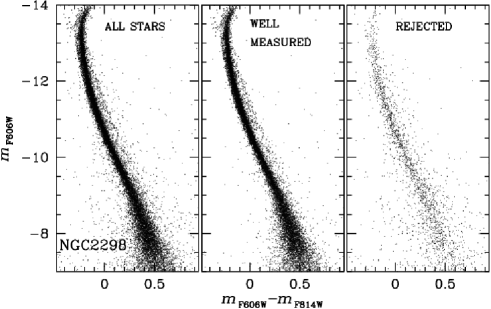
Figure 3: CMD of all the measured stars (left), of stars that passed our criteria of selection (middle), and CMD of rejected stars (right)

We began by dividing all the stars of each cluster into bins of 0.4 magnitude; for each of them, we computed the median values of the parameters ${\it rms_{\rm X,Y}}$ and ${\it q_{\rm F606W,F814W}}$ defined above and the $68.27^{\rm th}$ element of the percentile distribution (hereafter $\sigma$). We added to the median of each bin four times $\sigma$, and fitted these points with a spline to obtain the red lines of Fig. 2. All stars below the red line have been flagged as ‘well-measured’ according to that diagnostic.

The parameters ${\it o}_{\rm F606W}$ and ${\it o}_{\rm F814W}$ do not show a clear trend with magnitude. We flagged as ‘well-measured’ all the stars with ${\it o}_{\rm F606W}<1$ and ${\it o}_{\rm F814W}<1$.

In Fig. 3 we compare the color-magnitude diagram (CMD) of all the measured stars of NGC 2298 ($left$), the CMD of stars that pass all the selection criteria ($middle$), and the CMD of rejected stars ($right$). The sample of stars that have been used in the analysis that follows includes stars flagged as ‘well-measured’ with respect to all the parameters we used as diagnostics of the photometric quality.

The photometric catalog by Anderson et al. (2008) also provides the rms of the ${\it m}_{\rm F606W}$ and ${\it m}_{\rm F814W}$ magnitude measures made in different exposures. However, a star can have a large magnitude rms either because of poor photometry or because it is a binary system with short period photometric variability. In order to avoid the exclusion of this class of binaries, we have not used the rms of magnitude measures as diagnostics of the photometric quality in the selection of our stellar sample.

2.2 Artificial-star tests

Artificial-star (AS) tests played a fundamental role in this analysis; they allowed us to determine the completeness level of our sample, and to measure the fraction of chance-superposition ”binaries”. The GC Treasury reduction products (see Anderson et al. 2008) also contain a set of AS tests. The artificial stars were inserted with a flat luminosity function in F606W and with colors that lie along the MSRL for each cluster. Typically, $10^{5}$ stars were added for each cluster, with a spatial density that was flat within the core, and declined as $r^{-1}$ outside of the core. The stars were added one at a time, and as such they will never interfere with each other.

Each star in the input AS catalog is added to each image with the appropriate position and flux. The AS routine measures the images with the same procedure used for real stars and produces the same output parameters as in Sect. 2. We considered an artificial star as recovered when the input and the output fluxes differ by less than 0.75 magnitudes and the positions by less than 0.5 pixel. We applied to the recovered ASs the same criteria of selection described in Sect. 2 for real stars and based on the rms in position and on the ${\it q}_{\rm F606W,F814W}$ and ${\it o}_{\rm F606W,F814W}$ parameters. In what follows, including the completeness measure, we used only the sample of ASs that passed all the criteria of selection.

Since completeness depends on crowding as well as on stellar luminosity, we measured it applying a procedure that accounts for both the stellar magnitude and the distance from the cluster center. We divided the ACS field into 5 concentric annuli and, within each of them, we examined AS results in 9 magnitude bins, in the interval $-14<{\it m}_{\rm F814W}<-5$. For each of these 9 $\times$ 5 grid points we calculated the completeness as the ratio of recovered to added stars within that range of radius and magnitude. Finally, we interpolated the grid points and derived the completeness value associated with each star. This grid allowed us to estimate the completeness associated to any star at any position within the cluster. Results are shown in Fig. 4 for NGC 2298. The stars used to measure the binary fraction have all completeness larger than 0.50.

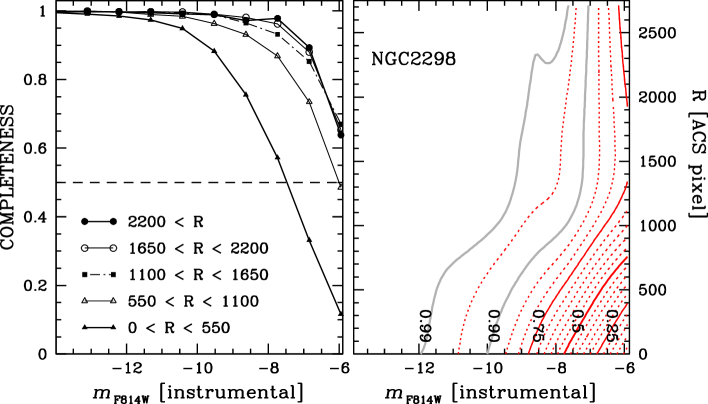
Figure 4: Left: Completeness as a function of the $m_{\rm F814W}$ magnitude in five annuli (the inner and outer radius of each annulus, in ACS pixels, are quoted in the inset) for NGC 2298. Right: Completeness contours in the radial distance versus $m_{\rm F814W}$ magnitude plane. The completeness levels corresponding to the red and gray continuous lines are quoted in the figure. Dotted lines indicate differences of completeness of 0.05 ranging from 0.05 to 0.95.

3 Photometric zero point variations

In some clusters, the distribution of foreground dust can be patchy, which causes a variation of the reddening with position in the field, resulting in a non-intrinsic broadening of the stellar sequences on the CMDs. In addition to these spreads, small unmodelable PSF variations, mainly due to focus changes, can introduce slight shifts in the photometric zero point as a function of the star location in the chip (see Anderson et al. 2008 for details). The color variation due to inaccuracies in the PSF model is usually $\sim$0.005 (Anderson et al. 2008, 2009, Milone et al. 2010). In some clusters, differential reddening effects may be much larger. An appropriate correction for these effects is a fundamental step, as it can greatly sharpen the MS, with a consequent improved analysis of the MS binary fraction.

3.1 Differential reddening

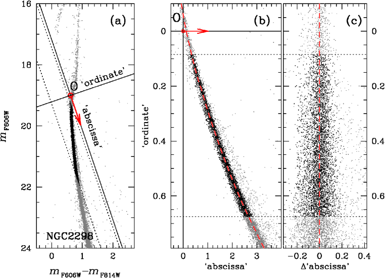
Figure 5: Panel a: observed CMD of NGC 2298; the arrow indicates the direction of reddening. The continuous lines are the axes (‘abscissa’ and ‘ordinate’) of the reference frame introduced in the procedure for the measurements of reddening variations. The position of NGC 2298 stars in this reference frame is shown in panel b where we draw the fiducial line of the MS as a dashed red line. Stars between the dotted lines (black points) have been used as reference stars. Panel C shows the rectified ‘ordinate’ vs. $\Delta$‘abscissa’ diagram.

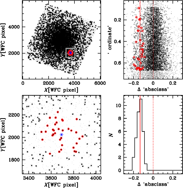
Figure 6: Visualization of the local approach for the estimate of the differential reddening suffered by the target star indicated with the blue asterisk. Upper left: Position of NGC 2298 stars in the ACS/WFC field of view (gray points). Red circles highlight the 35 reference stars in the lower left panel. Reference stars are indicated with black crosses, among them, the 35 closest neighbours (of the target star) are marked with red circles. The lower left panel is a zoom of a 700$\times$700 pixel centered on the target star. Upper right: ‘ordinate’ vs. $\Delta$ ‘abscissa’ for all the stars in the NGC 2298 field of view. The median $\Delta$ ‘abscissa’ of the 35 closest neighbor is indicated by the continuous red vertical line and corresponds to the differential reddening value suffered by the target star. The histogram of the $\Delta$ ‘abscissa’ distribution of the 35 closest neighbors is shown in the bottom right panel.

In order to correct for differential reddening, we started by defining a photometric reference frame where the abscissa is parallel to the reddening line, as shown in Fig. 5 for NGC 2298. To do this, we have first arbitrarily defined a point (O), near the MSTO in the CMD of $Panel\leavevmode\nobreak\ a$. Then we have translated the CMD such that the origin of the new reference frame corresponds to O. Finally, we have rotated the CMD counterclockwise by an angle:

$\theta={\rm arctan}\frac{A_{\rm F606W}}{A_{\rm F606W}-A_{\rm F814W}}$

as shown in Fig. 5b. The two quantities $A_{\rm F606W}$ and $A_{\rm F814W}$ are the absorption coefficients in the F606W and F814W ACS bands corresponding to the average reddening for each GC. They are derived by assuming, for each GC, the average $E(B-V)$ listed in the Harris (1996, 2003) catalog and linearly interpolating among the reddening and the absorption values given in Table 3 of Bedin et al. (2005) for a cool star. The reason for rotating the CMD is that it is much more intuitive to determine a reddening difference on the horizontal axis rather than along the oblique reddening line.

The value of $\theta$ depends weakly on the stellar spectral type, but this variation can be ignored for our present purposes. For simplicity, in this section, we will indicate as ‘abscissa’, the abscissa of the rotated reference frame, and as ‘ordinate’, its ordinate.

At this point, we adopt an iterative procedure that involves the following four steps:

1. We generate the red fiducial line shown in Fig. 5b. In order to determine this line, we used only MS stars. We divided the sample of these MS reference stars into ‘ordinate’ bins of 0.4 mag. For each bin, we calculated the median ‘abscissa’ that has been associated with the median ‘ordinate’ of the stars in the bin. The fiducial has been derived by fitting these median points with a cubic spline. Here, it is important to emphasize that the use of the median allows us to minimize the influence of the outliers as contamination by binary stars left in the sample, field stars or stars with poor photometry.

2. For each star, we calculated the distance from the fiducial line along the reddening direction ($\Delta$ ‘abscissa’). In the right panel of Fig. 5, we plot ‘ordinate’ vs. $\Delta$ ‘abscissa’ for NGC 2298.

3. We selected the sample of stars located in the regions of the CMD where the reddening line define a wide angle with the fiducial line so that the shift in color and magnitude due to differential reddening can be more easily separated from the random shift due to photometric errors. These stars are used as reference stars to estimate reddening variations associated to each star in the CMD and are marked in Fig. 5 as heavy black points.

4. The basic idea of our procedure, which is applied to each star (target) individually, is to measure the differential reddening suffered by the target star by using the position in the ‘ordinate’ vs. ‘abscissa’ diagram of a local sample of reference stars located in a small spatial region around the target with respect to the fiducial sequence.

   We must adopt an appropriate size for the comparison region in order to obtain the best possible reddening correction. The optimal size is a compromise between two competing needs. On one hand, we want to use the smallest possible spatial cells, so that the systematic offset between the ’abscissa’ and the fiducial ridgeline will be measured as accurately as possible for each star’s particular location. On the other hand, we want to use as many stars as possible, in order to reduce the error in the determination of the correction factor.

   As a compromise, for each star, we typically selected the nearest 30-100 reference stars and calculate the median $\Delta$ ‘abscissa’ that is assumed as the reddening correction for that star. In this way, our differential reddening correction will be done at higher spatial frequencies in the more populated parts of the observed field. In calculating the differential reddening suffered by a reference star, we excluded this star in the computation of the median $\Delta$ ‘abscissa’. As an example, in Fig. 6 we illustrate this procedure for a star in the NGC 2298 catalog. The position of all the stars within the ACS/WFC field of view is shown in the upper-left panel where reference stars are represented by black crosses, and the remaining stars are indicated with gray points. Our target is plotted as a blue asterisk. The 35 closest neighboring reference stars are marked with red circles. The lower-left panel is a zoom showing the location of the selected stars in a 700$\times$700 pixel box centered on the target. The positions of the 35 closest neighboring reference stars in the ‘ordinate’ vs. $\Delta$ ‘abscissa’ plane are shown in the upper right panel, and their histogram distribution is plotted in the bottom-right one. Clearly, neighboring stars define a narrow sequence with $\Delta$ ‘abscissa’ $\sim$$-$0.15. Their median $\Delta$ ‘abscissa’, which is indicated by the continuous red line, is assumed to be the best estimate of the differential reddening suffered by the target star.

After the median $\Delta$‘abscissa’ have been subtracted to the ‘abscissa’ of each star in the rotated CMD, we obtain an improved CMD which has been used to derive a more accurate selection of the sample of MS reference stars and derive a more precise fiducial line. After step 4, we have a newly corrected CMD. We re-run the procedure to see if the fiducial sequence needs to be changed (slightly) in response to the adjustments made and iterated. Typically, the procedure converges after about four iterations. Finally, the corrected ‘abscissa’ and ‘ordinate’ are converted to $m_{\rm F606W}$ and $m_{\rm F814W}$ magnitudes.

From star-to-star comparison of the original and the corrected magnitudes we can estimate star to star variations in $E(B-V)$ and derive the reddening map in the direction of our target GCs. As an example, in Fig. 7, we divide the field of view into 8 horizontal slices and 8 vertical slices and plot $\Delta\leavevmode\nobreak\ E(B-V)$ as a function of the Y (upper panels) and X coordinate (right panels). We have also divided the whole field of view into 32$\times$32 boxes of 128$\times$128 ACS/WFC pixels and calculated the average $\Delta\leavevmode\nobreak\ E(B-V)$ within each of them. The resulting reddening map is shown in the lower-left panel where each box is represented as a gray square. The levels of gray are indicative of the amount of differential reddening as shown in the upper right plot. The analysis of the intricate reddening structures in our GC fields is beyond the purposes of the present work and will be presented in a separate paper (King et al., in preparation).

Fig. 8 shows the CMDs of twelve of the GCs studied in this paper including NGC 2298. These are the clusters that revealed the largest differential reddening $\Delta E({\it m}_{\rm F606W}-{\it m}_{\rm F814W})>0.05$.

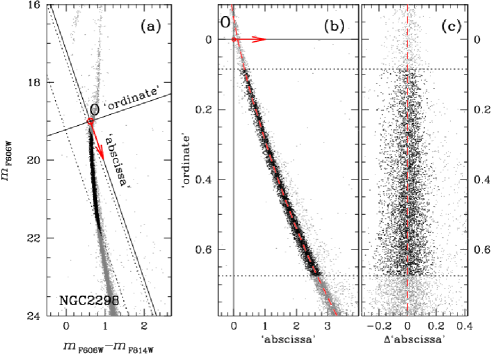
Figure 7: Bottom-left: Map of differential reddening in the NGC 2298 field of view. The gray levels correspond to the magnitude of the variation in local reddening as indicated in the upper-right panel. We divided the field of view into 8 horizontal slices and 8 vertical slices. Upper-left and lower-right panels plot $\Delta\leavevmode\nobreak\ E(B-V)$ as a function of the Y and X coordinate.

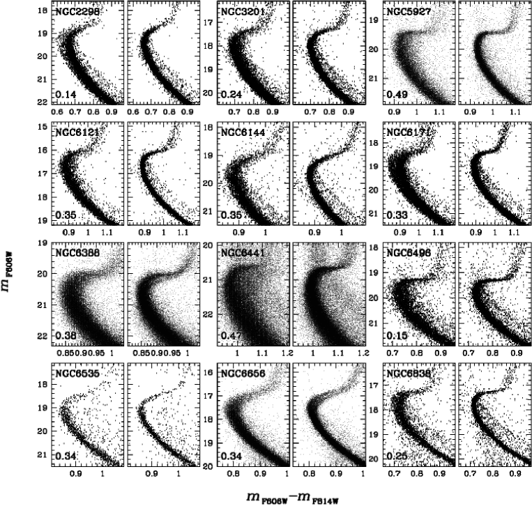
Figure 8: CMDs of twelve GCs before (left) and after (right) the correction for differential reddening. For each cluster we give the average reddening from the Harris (1996) catalog.

3.2 PSF Variations

Some GCs have a reddening that is close to zero and therefore we expect negligible variations of reddening within their field of view. In these cases, we need to apply only a correction for the photometric zero point spatial variation due to small, unmodelable PSF variations. Usually, these PSF variations affect each filter in a different way, so their most evident manifestation is a slight shift in the color of the cluster sequence as a function of the location in the field (Anderson et al. 2008). For this reason, when the average reddening of the cluster (from Harris 1996) is lower than 0.10 mag, we did not follow the recipes for the correction of differential reddening described in the previous section, but corrected our photometry for the effects of the variations of the photometric zero point along the chip. We used a procedure that slightly differs from the one of Sect. 3.1. The only difference from what done in GCs with high reddening is that we did not rotated the CMD and so we did not apply the correction along the reddening line, but along the color direction.

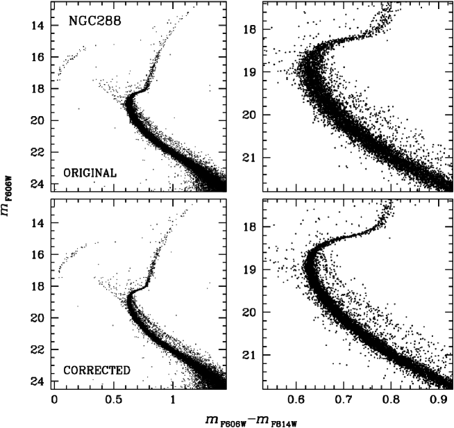
Figure 9: CMDs of NGC 288 before (top) and after (bottom) correction for photometric zero points variations. Right panels show a zoom of CMD around the SGB and upper-MS region.

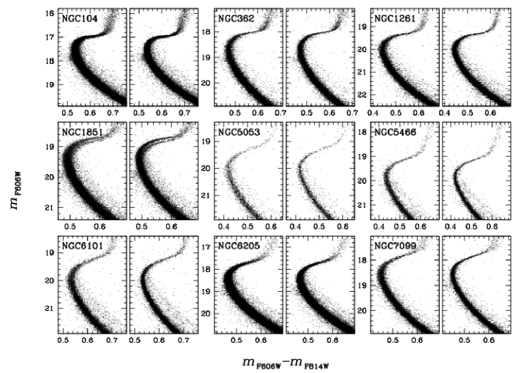
Figure 10: Comparison of the CMD of nine GCs studied in this paper before (left) and after (right) the correction for photometric zero points variations.

The results of this procedure are illustrated in Fig. 9 where we compare the original and the correct CMD of NGC 288. The improvement in the quality of our CMD is exemplified by the comparison in right panels figures that show a zoom of the SGB and the upper-MS.

Other examples of the improvement in the photometry coming from this procedure are shown in Fig. 10 where we plot the nine GCs studied in this paper for which we measured the largest color variations. The average color variations are typically around 0.005 mag for each cluster with $E(B-V)<$0.10 studied in this paper and never exceed 0.035 mag.

4 The measure of the fraction of binaries with high mass ratio

Binaries with large mass ratios have a large offset in luminosity from the MSRL and are relatively easy to detect. On the contrary, a small mass ratio doesn’t pull them very far off of the MSRL, making them hard to distinguish from single MS stars. Finally, the low signal to noise photometry of faint stars limits the range where binaries can be detected and studied.

In practice, the limited photometric precision and accuracy makes impossible the direct measure of the overall population of binaries without assuming a specific distribution of mass ratios f(q). For this reason, in this paper, we followed two different approaches to study the binary population in our target GCs.
1) We isolated different samples of high mass-ratio binaries (i. e. the binary systems with $q>$ 0.5, 0.6 and 0.7). For them, we obtained a direct measure of their fraction with respect to the total number of MS stars, and studied the properties of each group (Sect. 4).
2) We determined the total fraction of binaries by assuming a given f(q) (Sect. 5.2).

In each cluster, we estimated the fractions of high q binary stars in the F814W magnitude interval ranging from 0.75 (${\it m}_{\rm F814W,bright}$) to 3.75 (${\it m}_{\rm F814W,faint}$) magnitudes below the MSTO. In this work we used the MSTO magnitudes from Marín-Franch et al. (2009), who used our same photometric data base. The choice of this magnitude interval represents a compromise between the necessity of a large set of stars and the need to avoid faint stars to be able to measure the binary fraction also in clusters with poorer photometry (because of crowding).

To illustrate our setup, Fig. 11 shows the various regions we studied in the CMD of NGC 2298 in order to measure the fraction of binaries with mass ratio ${\it q}>0.5$ for this cluster. The upper half of the figure displays two regions of the CMD: Region A (upper left) and region B (upper right).

Region A includes all the stars that we can consider to be cluster members. It includes: all the single MS stars and the MS+MS binaries with a primary star that have ${\it m}_{\rm F814W,bright}<{\it m}_{\rm F814W}<{\it m}_{\rm F814W,faint}$. The green continuous line is the MS fiducial line, drawn as described in Sect. 3. To include stars that have migrated to the blue due to measuring error, we extend region A up to the green dashed line, which is displaced to the blue from the MSRL by 3 times the the average color error for a star at that magnitude. The red dotted line is the locus of MS-MS binaries whose components have equal mass; we set the limit of region A by drawing the red dot-dashed line, displaced to the red from the dotted line by 3 times the rms color error. The upper-right panel of Fig. 11 shows Region B, which is chosen in such a way that it contains all the binaries with ${\it q}>0.5$. It starts at the locus of binaries with mass ratio, q=0.5, marked by the continuous red line and ends at the dotted-dashed red line, which is the same line defined in the upper-left panel.

The lower half of Fig. 11 shows where observed stars and ASs fall within these two regions. The left-lower panel plots the observed stars and the middle panel shows ASs. We note that a significant number of ASs fall in region B. Only a fraction of them can be explained by photometric errors; in many cases two stars fell at positions so close together that a pair of stars has blended into a single object, which would simulate a binary. Obviously, in the real CMD, regions A and B are also populated by field stars, as shown in the right panel for NGC 2298. We will explain how the field star CMD is built in Sect. 4.1.

To determine the fraction of binaries with q$>$0.5 we started by measuring the number of stars, corrected for completeness, in regions A ($N_{\rm REAL}^{\rm A}$) and B ($N_{\rm REAL}^{\rm B}$). They are calculated as $N_{\rm REAL}^{\rm A(B)}=\sum_{1}^{N_{\rm OBS}^{A,(B)}}{1/c_{\rm i}}$, where ${\it N}_{\rm OBS}^{\rm A,(B)}$ is the number of stars observed in the region A (B) and ${\it C}_{\rm i}$ is the completeness (coming from AS tests). Then, we evaluated the corresponding numbers of artificial stars ($N_{\rm ART}^{\rm A}$ and $N_{\rm ART}^{\rm B}$) and field stars ($N_{\rm FIELD}^{\rm A}$ and $N_{\rm FIELD}^{\rm B}$). In the following Sects. 4.1 and 4.2 we will describe the methods that we used to estimate $N_{\rm FIELD}^{\rm A}$ and $N_{\rm FIELD}^{\rm B}$ and $N_{\rm ART}^{\rm A}$ and $N_{\rm ART}^{\rm B}$.

The fraction of binaries with q$>$0.5 is calculated as

$$f_{\rm bin}^{\rm q>0.5}=\frac{N_{\rm REAL}^{\rm B}-N_{\rm FIELD}^{\rm B}}{N_{\rm REAL}^{\rm A}-N_{\rm FIELD}^{\rm A}}-\frac{N_{\rm ART}^{\rm B}}{N_{\rm ART}^{\rm A}}.$$ (1)

Similarly, we have calculated the fraction of binaries with q $>$0.6 and q$>$0.7. To do this it is necessary to move redward the left-hand side (red solid line) of Region B, according to what is shown in Fig. 1.

The error associated to each quantity of eq. 1 is the Poisson error and the error on the obtained binary fraction is calculated by following the standard errors propagation. Therefore it represents a lower limit for the uncertainty of the binary fraction. We note that the binary fractions strongly differ from one cluster to another with $f_{\rm bin}^{\rm q>0.5}$ ranging from $\sim$0.01 to $\sim$0.40.

In order to analyze the radial distribution of binary stars in GCs and provide information useful for dynamical models of our target clusters, we have calculated both the total binary fraction and the fraction of binaries with $q>0.5$ at different radial distances from the cluster center. More specifically, we defined three different regions:

• a circle with a radius of one core radius (${\it r}_{\rm C}$ sample);

• an annulus between the core and the half-mass radius (${\it r}_{\rm C-HM}$ sample);

• a region outside the half-mass radius (${\it r}_{\rm oHM}$ sample).

The values of the core radius and the half-mass radius are from the Harris (1996) catalog. It should be noted that, even if our data are homogeneous, in the sense that they came from the same instrument (ACS/WFC/HST) and have been reduced adopting the same techniques, their photometric quality vary from cluster to cluster, mainly because of the different stellar densities (which affects the crowding). For this reason, for some GCs that have poor photometry in their central regions, we have measured the fraction of binaries only outside a minimum radius ( $R_{\rm MIN}$) where it is possible to distinguish binaries with $q>0.5$ from single MS stars. The adopted values of $R_{\rm MIN}$ are listed in Table 2. The fractions of binaries with q$>$0.5, q$>$0.6, q$>$0.7 ($f_{\rm bin}^{\rm q>0.5}$, $f_{\rm bin}^{\rm q>0.6}$ and $f_{\rm bin}^{\rm q>0.7}$) for the clusters in our sample are listed in Cols. 3, 4, 5 of Table 2, respectively. In column 6 there is also our best-estimate of the total binary fraction (i. e. the fraction of binaries in the whole range $0<q<1$) that will be estimated in Sect. 5.2. We give both the fractions of binaries calculated over the ACS/WFC field and those in each of the three regions defined above.

Following these considerations, it was possible to include in the ${\it r}_{\rm C}$ sample only 43 out of the original 59 GCs. In addition, the limited ACS field of view reduced the number of GCs with ${\it r}_{\rm C-HM}$ and ${\it r}_{\rm oHM}$ samples to 51 and 45 clusters, respectively.

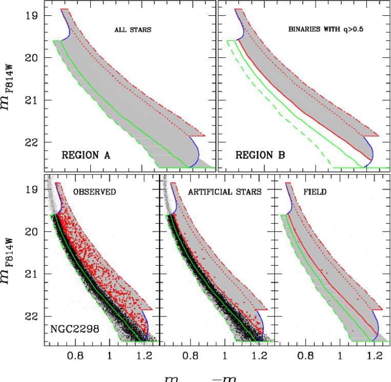
Figure 11: Gray areas in the upper panels are the regions A, and B of the NGC 2298 CMD adopted to select all the (single and binary) cluster stars (left) and the candidate binaries with q$>$0.5 (right), in a range of 3 $m_{\rm F814W}$ magnitudes. In all panels, the MSRL is represented as a green continuous line, while the green dashed line is blue shifted from the MSRL by three times the color error. The red continuous line is the locus of MS-MS binaries with mass ratio q=0.5, while the red dotted line is the locus of MS-MS binaries whose components have equal mass. The red dashed dotted line is displaced to the red from the dotted line by 3 times the color error. Lower panels show the observed CMD of NGC 2298 ($left$), the artificial stars CMD ($middle$), and the CMD of field stars ($right$).

4.1 Field contamination

The best ways to quantify foreground/background contamination of regions A and B consists in identifying field stars on the basis of their proper motion, which usually differs from the cluster motion. For several clusters of the sample considered in this paper there are previous epoch HST images with a sufficiently long temporal baseline and precision to allow the measurement of proper motions. We used archive material to determine the proper motions of 20 GCs that are critically contaminated by field stars: ARP 2, NGC 104, NGC 362, NGC 5286, NGC 5927, NGC 6121, NGC 6218, NGC 6352, NGC 6388, NGC 6441, NGC 6397, NGC 6496, NGC 6535, NGC 6626, NGC 6637, NGC 6652, NGC 6656, NGC 6681, NGC 6838, and TERZAN 7. The procedure to measure proper motions is outlined in Sect. 4.1.1

In order to determine field objects contamination in the CMDs of the remaining clusters, we run a program developed by Girardi et al. (2005), which uses a model to predict star numbers in any Galactic field. Details of this procedure are given in Sect. 4.1.2.

4.1.1 Proper motions

Proper motions are measured by comparing the positions of stars measured at two or more different epochs. For the majority of the clusters only two epochs were available and we followed a method that has been widely described in many other papers (e. g. see Bedin et al. 2008, Anderson & van der Marel 2010). In the cases of NGC 104, NGC 362, NGC 5927, NGC 6121, NGC 6397, and NGC 6656 we used a sample of images taken at three or even more different epochs and determined proper motions with the procedure given by McLaughlin et al. (2006). We refer the interested reader to these paper for a detailed description.

Results are shown in Fig. 12 which plots proper motions for twenty GCs. We plotted only stars in the F814W magnitude range indicated by the numbers quoted in the insets Since we measured proper motions relative to a sample of cluster members, the zero point of the motion is the mean motion of the cluster. Therefore, the bulk of stars clustered around the origin of the vector-point diagrams (VPD) consists mostly of cluster members, while field stars are distributed over a larger range of proper motions.

Proper motions offer a unique opportunity to estimate the number of field stars that populate the regions A and B of the CMD. In order to identify field objects, we began to isolate stars whose proper motions clearly differ from the cluster mean motion by using the procedure that is illustrated in Fig. 13 for NGC 6656 (where cluster and field stars are well separated in the VPD), and in Fig. 14 for NGC 6838 (where the separation is less evident).

In the left panel of Figs. 13 and  14 we show the CMD for all the stars for which proper motions measurements are available. The second column of the two figures shows the VPD of the stars in four different magnitude intervals. The red circle is drawn to identify the stars that have member-like motions. In the following, we will indicate as $R_{\rm CL}$ and $R_{\rm OUT}$ the VPD regions within and outside the red circles. We fixed the radius of the circles at 3.25 $\sigma$, where $\sigma$ is the average proper-motion dispersion in the two dimensions. If we assume that proper motions of cluster stars follow a bivariate Gaussian distribution, the circle should include 99.5 % of the members in each magnitude interval. The third panel shows the CMD of stars with cluster-like proper motion, while selected field objects are plotted on the right panel.

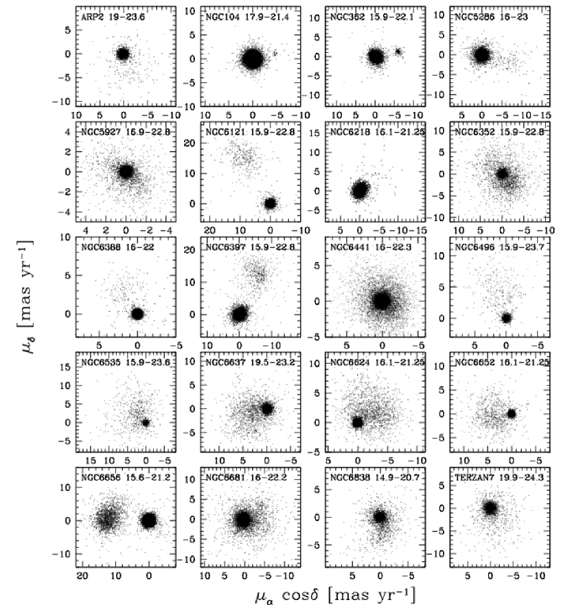
Figure 12: Vector-point diagram of proper motions, in equatorial coordinates, for twenty GCs. Only stars in the ${\it m}_{\rm F814W}$ interval indicated in each panel are shown.

Figure 13: Leftmost column: ${\it m}_{\rm F814W}$ vs. ${\it m}_{\rm F606W}-{\it m}_{\rm F814W}$ CMD for all the stars of NGC 6656 with available measures of proper motions. Second Column: Proper motion diagrams of the stars in the left panels in $masyr^{-1}$, in intervals of 1.4 mag. Third column: The proper motion selected CMD of cluster members. Rightmost column: The CMD of field stars.

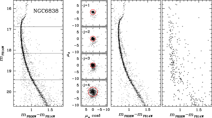
Figure 14: As in Fig. 13, but for NGC 6838.

We emphasize here that, as we will see in detail in the following, proper motions are used to evaluate the numbers of field stars that randomly fall within the CMD regions A and B ($N_{\rm FIELD}^{\rm A,B}$) and not to isolate a sample of cluster stars. This approach will allow us to determine the binary fraction by means of eq. 1 in the whole ACS/WFC field of view and not only in the spatial regions covered by multi-epochs images where proper motions are available. To determine the values of $N_{\rm FIELD}^{\rm A,B}$ we have to account for three factors:

1. To accurately measure $N_{\rm FIELD}^{\rm A,B}$ we need a correct estimate of the fraction of field stars that share cluster-like proper motions.

2. Proper motions are not available for the whole ACS/WFC field of view because, usually, there is only a partial overlap between the images at different epochs. As a consequence of this we need an accurate measurement of the area of the overlapping region.

3. Proper motions may not be available for a fraction of stars in the ACS/WFC catalogs even if they are in the overlapping region because these stars are not measured in the second-epoch images (that in many cases come from WFPC2), because they either are too faint or in a too crowded region.

Specifically the number of field stars in the region A has been evaluated as

$$N_{\rm FIELD}^{\rm A}=\sum_{\rm j=1}^{4}\frac{1+n^{\rm R_{\rm CL}}_{\rm FIELD,j}/n_{\rm FIELD,j}}{F_{\rm AREA}}\sum_{\rm i=1}^{n_{\rm FIELD,j}^{\rm A}}\frac{1}{f_{\rm PM}^{\rm i}\ c_{\rm i}}$$ (2)

where:

• $n_{\rm FIELD,j}$ and $n_{\rm FIELD,j}^{\rm A}$ are the total number of field objects and the number of field objects within Region A for which we have measured proper motions, in the magnitude interval j (see the rightmost column of Figs. 13 and  14), respectively.

• $n^{\rm R_{\rm CL}}_{\rm FIELD,j}$ is the fraction of field objects that share proper motions similar to the cluster;

• $F_{\rm AREA}$ is the fraction of the ACS/WFC field of view with multi-epoch observations;

• $c_{\rm i}$ is the completeness of the ACS/WFC catalog calculated in Sect. 2.2;

• $f_{\rm PM}^{\rm i}$ is a factor that accounts for the availability of proper motions (as in point 3 above).

And the same is done to evaluate the number of field stars in the Region B. In the following, we describe the procedure used to determine $n^{\rm R_{\rm CL}}$, $F_{\rm AREA}$, and $f_{\rm PM}^{\rm i}$.

Field stars with cluster-like proper motions
The VPDs of Fig. 12 show that almost all the clusters have some field stars that share the mean cluster motion. The fraction of these sources with respect to the cluster stars depends on several factors, such as the astrometric quality of the data, the temporal baseline, the line of sight, and the motion of the cluster with respect to the field. Their fraction is almost negligible in NGC 6656 and other cases, but makes a significant contribution to the binary fraction in most of the GCs of Fig. 12. We now describe a method to determine the fraction of field stars with cluster-like proper motion in order to accurately infer ${\it N}_{\rm FIELD}^{\rm A}$ and ${\it N}_{\rm FIELD}^{\rm B}$ in equation 1.

We note that, for the purposes of this paper, we do not need to isolate these intruders. It is sufficient to estimate their total amount, and, more specifically, the amount of field stars with cluster-like motions that populate the CMD region associated with MS-MS binaries or MS single stars.

We independently calculated, for the GCs with reliable proper motions, the number of field stars with cluster-like proper motions for each of the four magnitude intervals of Figs. 13, and  14. In the cases of GCs where cluster and field stars are clearly separated in the proper motion diagram (ARP 2, NGC 104, NGC 362, NGC 5286, NGC 6121, NGC 6218, NGC 6388, NGC 6397, NGC 6496, NGC 6535, NGC 6637, NGC 6624, NGC 6652, NGC 6656, and Terzan 7) we used the method that is illustrated in Fig. 15 for NGC 6656. All the field and cluster stars with reliable proper motions are located within the dotted circle of the left panel VPD We considered as probable cluster members all the objects that are plotted as thin gray dots in the yellow area (region ${\it R_{\rm CL}})$ of the zoomed VPD in the right panel, while remaining objects are flagged as field stars and are represented as heavier points.

The distribution of field stars in the VPD is clearly elongated and the isodensity contours can be approximately described by ellipses. In Fig. 15 we show the two isodensity contours that are tangent to the region ${\it R}_{\rm CL}$ and define the red region (${\it R}_{\rm T}$). The number of field stars within ${\it R}_{\rm CL}$ is assumed to be:
$n_{\rm FIELD}^{\rm R_{\rm CL}}=n_{\rm R_{\rm T}}S_{\rm R_{\rm CL}}/S_{\rm R_{\rm T}}$
where $S_{\rm R_{\rm CL}}$ and $S_{\rm R_{\rm T}}$ are the areas of regions ${\it R}_{\rm CL}$ and ${\it R}_{\rm T}$ and $n_{\rm R_{\rm T}}$ is the number of stars within ${\it R}_{\rm T}$.

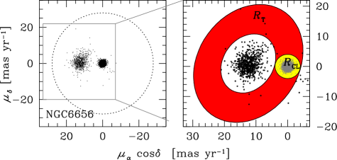
Figure 15: Setup to estimate the fraction of field stars with cluster-like proper motions in NGC 6656.

In the cases of NGC 5927, NGC 6352, NGC 6441, NGC 6681, and NGC 6838, where the separation of field and cluster stars is less evident, we followed a different recipe, which is illustrated in in Fig. 16 for NGC 6838. The upper panels show the CMD (left) and the VPD (right) for stars in the third interval of magnitudes (j=3) of Fig. 14. We selected, on the CMD, a sample of stars that, on the basis of their color and magnitude, are probable background/foreground objects. These stars are marked as heavy black points in the lower CMD of Figure 16, while in the right-lower panel we show their position in the VPD.

If we assume that the fraction of selected objects within $R_{\rm CL}$ with respect to the total number of selected field objects ($f^{\rm R_{CL}}_{\rm FIELD}$) is representative of the overall fraction of field stars that share cluster proper motions we can impose: $n_{\rm FIELD}^{\rm R_{\rm CL}}=n_{\rm FIELD}f^{\rm R_{CL}}_{\rm FIELD}$. The contribution of $n_{\rm FIELD}^{\rm R_{\rm CL}}$ to the measure of the binary fraction is, for all the clusters smaller than 0.01.

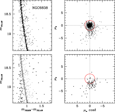
Figure 16: Estimate of the contamination of field stars that share cluster proper motions in NGC 6838. Upper panels show the CMD (left) and the VPD (right) for stars with 18.15$<$${\it m}_{\rm F814W}$$<$19.45. Lower panels display the CMD (left) and the VPD (right) for those objects that, on the basis of their position on the CMD, are probable field stars.

In order to investigate the reliability of this approach, we applied it also to the 15 GCs for which proper motions allow us to almost completely separate cluster stars from field ones. In all cases, we found full consistency between the two approaches, with the the fraction of binaries with q$>$0.5 listed in Table 2 differing by less than 0.01.

The spatial coverage of multi-epoch images
For most clusters, there is only a partial overlap among the different epoch images. In the following we will refer to the region that has been observed in at least two epochs as ‘${\it R}_{\rm II}$’. Fig. 17 shows the example for NGC 6656, where we indicate as light gray points all the stars for which we have only photometry, and mark with black points the stars with both photometric and proper motion measurements. As our field is just a few square arcmins, we can assume that the background/foreground population is uniformly distributed within it, and therefore we estimate the total number of field stars in our field of view as the product of the number of field stars in the region $R_{\rm II}$ and the ratio between the area of the total field of view and the area of $R_{\rm II}$. In this paper, we will refer to this ratio as: $F_{\rm AREA}$.

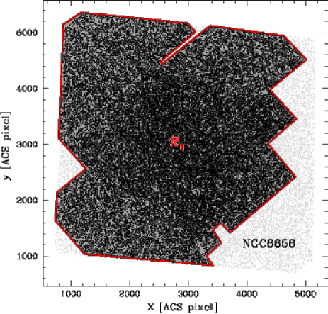
Figure 17: Map of all the stars NGC 6656 (light gray points) with ${\it m}_{\rm F814W}<$18.25. Black points mark all the stars with available proper motions. The contour of region ‘${\it R}_{\rm II}$’ is colored in red.

Completeness correction for field stars
In the procedure that we have applied to determine the cluster membership using proper motions, we have automatically excluded all the stars that might be members but have poor astrometry. An accurate estimate of the fraction of these stars is necessary to infer the correct values of ${\it N}_{\rm FIELD}^{\rm A}$ and ${\it N}_{\rm FIELD}^{\rm B}$. To estimate the fraction of cluster stars lost by applying the proper motion selection criteria, we applied the procedure illustrated in Fig. 18 for NGC 6656. In panel $a$ we show the ${\it m}_{\rm F814W}$ vs. ${\it m}_{\rm F606W}-{\it m}_{\rm F814W}$ CMD for all the stars in the region ‘$R_{\rm II}$’. Proper motion measurements are available only for a fraction ($f_{\rm PM}$) of these stars. Their CMD is shown in panel $b$, while the CMD for stars with no available proper motions is plotted in panel ($c$).

To determine $f_{\rm PM}$ we started by dividing the CMD into bins of 0.5 ${\it m}_{\rm F814W}$ magnitudes. In each of them, we counted the total number of observed stars (${\it N}_{\rm OBS}$) and the number of star with a reliable estimate of proper motions (${\it N}_{\rm PM}$). The fraction of stars with a proper motions in that bin is: ${\it f}_{\rm PM}={\it N}_{\rm PM}/{\it N}_{\rm OBS}$.

We then calculated the median ${\it m}_{\rm F814W}$ magnitude of the observed stars (${\it m}_{\rm MED}$) in each bin. We associated to each bin the corresponding value of ${\it f}_{\rm PM}$ and ${\it m}_{\rm MED}$. The (${\it f}_{\rm PM}^{\rm i}$) for each i-star is calculated by interpolation with a spline. In panel ($d$) of Fig. 18 we show the final ${\it f}_{\rm PM}$ as a function of ${\it m}_{\rm F814W}$. For the GCs studied here always we have ${\it f}_{\rm PM}>0.4$ at the level of 3.75 F814W magnitudes below the MSTO.

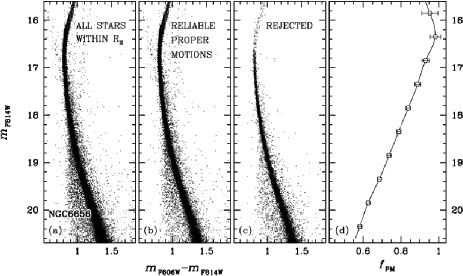
Figure 18: Panel a: CMD for all the stars within the region ‘$R_{\rm II}$’; Panel b: CMD for stars with a reliable estimate of proper motions; Panel c: CMD for stars within ‘$R_{\rm II}$’ for which there are not reliable measurements of proper motions; Panel d: Fraction of stars with good proper motions with respect to the total number of stars within ‘$R_{\rm II}$’ as a function of ${\it m}_{\rm F814W}$.

4.1.2 Galactic model

In order to estimate the number of background/foreground stars in the field of view of the GCs studied in this paper, and for which we do not have reliable measurements of proper motions, we used the theoretical Galactic model described by Girardi et al. (2005). This model was used to generate a synthetic CMD (in the ACS/WFC F606W and F814W bands) containing the expected field stars in the cluster area that we are studying. The synthetic CMDs were used to count the number of field stars in the CMD regions A, and B (${\it N}_{\rm SIM}^{\rm A}$, ${\it N}_{\rm SIM}^{\rm B}$) defined in Fig 11. Obviously, the number of stars in simulated CMDs may differ from that of observed field stars. To minimize the effect of such uncertainties on the measure of the fraction of binaries in GCs, we defined in the CMD a region F on the red side of equal-mass binaries fiducial sequence, that is delimited on the blue side by the red dashed-dotted line of Fig. 11 and is likely not populated by cluster stars, as illustrated in Fig. 19 for NGC 2298. We determined the numbers of stars within F in the observed and in the simulated CMDs (${\it N}_{\rm OBS}^{\rm F}$ and ${\it N}_{\rm SIM}^{\rm F}$ respectively).

The number of field stars in the CMD regions A is then calculated as:

$${\it N}_{\rm FIELD}^{\rm A}={\it N}_{\rm SIM}^{\rm A}{\it N}_{\rm OBS}^{\rm F}/{\it N}_{\rm SIM}^{\rm F}$$ (3)

and a similar equation is used to estimate the number of field stars in the region B.

As anticipated in Sect. 2, we removed from our list all clusters for which we had no proper motion (two epochs data) and for which Girardi et al. (2005) model was prediction a field star contamination larger than 1%, with the only exception of E3 (a 2.4% expected contamination) and NGC 6144 (1.3%). Therefore, for clusters for which we have to rely on a Galactic model to estimate the foreground//background stars, the contamination is expected to be minimal. On the other hand, we kept into the sample all cluster for which we could use proper motion to estimate field stars, independently from the level of contamination.

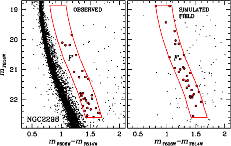
Figure 19: Observed CMD of NGC 2298 (left) and simulated CMD of field stars in the NGC 2298 field of view (right).

In order to investigate whether the estimate of field stars from Galactic models is reliable, we applied the synthetic CMDs method also in the 15 GCs for which we have reliable proper motion measurements. We found that, in the cases of GCs with a small field-star contamination, the fraction of binaries with q$>$0.5 derived following the two approaches is identical within the uncertainties, with differences smaller than 0.01. For some GCs with a significant background/foreground population, namely NGC 5927, NGC 6352, NGC 6388, NGC 6441, NGC 6637, and NGC 6681, the fractions of binaries derived using a Galactic model differ from those derived using proper motions by 0.01 to 0.03 (for NGC 6441).

4.2 Estimate of the fraction of apparent binaries

Chance superpositions of two physically unrelated stars that happen to lie nearly along the line of sight (apparent binaries) and superposition of a faint star and a positive background fluctuation may reproduce the color and luminosity of a genuine binary system, and populate the CMD region occupied by binaries. In a crowded stellar field, like the core of a GC, a reliable measure of the binary fraction requires good accuracy in deriving the number of chance superpositions.

We can identify and reject a significant fraction of these objects by analyzing the stellar profile, and the PSF-fit errors. For this reason, in this work, we limited our study to the objects that pass the selection criteria described in Sect. 2.1.

In order to account for the blends that have not been rejected, a statistical estimate of their number and distribution in the CMD is necessary. In this paper, we used extensive artificial-star test experiments to evaluate directly the effects of blends.

Specifically, in this subsection, we illustrate the procedure adopted to determine the relative numbers of artificial stars in the regions A and B of the CMD of Fig. 11 ($N_{\rm ART}^{\rm A}$ and $N_{\rm ART}^{\rm B}$) that are used to calculate the last term of eq. 1.

This analysis requires that the artificial star sample that we will compare to observed data reproduce as much as possible all the details of real stars. In particular we need the best possible match between the luminosities, the radial distribution and the photometric errors of observed and simulated stars.

The data set described in Anderson et al. (2008) includes an extensive set of artificial-star tests for each cluster. The same quality parameters were determined for the artificial stars as for the real stars, so we apply the same selection criteria to them as we did to the real stars in Sect. 2.1.

To apply these generic artificial-star tests to the real cluster distribution, for each real star observed, we took a set of the artificial stars within $\pm 0.10$ magnitude and with radial distances within $100$ pixels of that of the star. These are the stars that were used to estimate the measurement errors (random and systematic) of the stars in the cluster.

The result of this procedure is a catalog of simulated stars that reproduces both the radial and the luminosity distributions of real stars. Several effects contribute to the observed width of the main sequence. In addition to photon noise, we have the contribution of spatial variations of the PSF and residual differential reddening that are beyond the sensitivity of the method that we used to correct them, as well as scattered light, possible star-to star metallicity variations, etc. However, for the purposes of this work, it is not necessary to distinguish the contributions of the single sources of the broadening and we can include them in the photometric errors ($\sigma$).

Since MS-MS binary systems and apparent binaries both lie on the red side of the MS, we can use the MS scatter to the blue side of the MS as an estimate of the photometric error. We note that the blue portion of the MS may be contaminated by MS-white dwarf binaries but their influence on $\sigma$ is expected to be negligible, and further reduced by the applied ”kappa–sigma” rejection algorithm, as described below.

In order to estimate $\sigma$, we used the following iterative procedure, which has been applied to both the observed and artificial-star CMD. First of all, we subtracted the color of the MSRL from the color of each star. Then we divided this CMD into several intervals of magnitude, each one containing the same number of stars, and constructed a histogram of the color distribution for each magnitude interval. The size of each interval is a compromise between maximizing the number of stars to reduce the statistical errors and minimizing the magnitude intervals to account for the variations of the photometric error as a function of the luminosity. For these reasons, the size of the adopted interval varies from one cluster to another, depending on the number of sampled stars.

We used least-squares to fit each histogram with a Gaussian that had three fitting parameters: its center, its amplitude, and its dispersion $\sigma$. Then, we rejected all stars for which color is far more than $3\sigma$ from the fiducial line, because most of these objects must be field stars or binaries. Finally we used the remaining sample for a new Gaussian fit.

All the stars with negative color in the rectified CMD (i. e., those on the blue side of the MS) are used for a new Gaussian fit, but, this time, we fixed the center and the amplitude of the Gaussian and considered $\sigma$ as the only free parameter. The best fitting $\sigma$ is adopted as the average photometric error in that magnitude interval. The errors corresponding to a given magnitude in the CMD are obtained by interpolations.

As expected, the artificial star color distribution is narrower than the real star one. We need to properly estimate the difference between the artificial-star photometric error and the photometric error of real stars, since, as it will be clearer in next section, we need an artificial-star CMD with the correct photometric error in order to estimate the photometric outliers which contaminate the binary region.

The smaller color dispersion of the artificial star CMD comes from the fact that the measurement errors of artificial stars are smaller than the corresponding error of real stars. This difference is due to the fact that, in fitting artificial stars, we use exactly the same PSF that was used to originate them, while we cannot expect the same perfect match of the PSF with the real PSF of real stars. In addition, and for the same reason, artificial-star photometry is not affected by zero point photometric errors, and errors associated with the differential reddening correction.

The difference between the MS color spread of observed and simulated stars might be also due to multiple stellar populations. Indeed, nearly all the GCs studied so far host two or more generations of stars with a different light-elements. In few GCs, there are also star-to-stars iron variations (see Milone et al. 2010b for a recent review).

Among the clusters studied in this paper, multiple MSs associated to helium variation have been identified in 47 Tuc, NGC 6752, and NGC 6397 where the $m_{\rm F606W}-m_{\rm F814W}$ color difference between the He-rich and He-poor MS is about 0.01 mag (Anderson et al. 2009, Milone et al.  2010a, 2011b,c) i. e. has the same order of magnitude as the color errors of the best measured MS stars. NGC 6656 (M22) is the only cluster of this paper where two groups of stars with a different iron content have been identified. In this case theoretical isochrones show that the measured [Fe/H] difference of $\sim$0.15 dex do not produce any appreciable $m_{\rm F606W}-m_{\rm F814W}$ color bimodality among MS stars (Marino et al.  2009, 2011). In general the MSs corresponding to the different stellar populations observed in the majority of GCs (and hence formed by stars that could have different overall CNO abundance, and light elements variations) are almost overimposed when observed in the $m_{\rm F606W}-m_{\rm F814W}$ color (Sbordone et al. 2011).

As an example, the difference in color dispersion between the real and the artificial star CMDs of NGC 2298 are shown in Fig. 20.

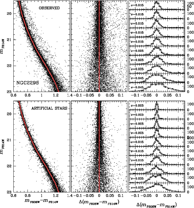
Figure 20: Left: The observed (top) and simulated (bottom) CMD of NGC 2298 with the fiducial line overplotted; Middle: The CMDs rectified by subtraction of the fiducial line; Right: Color distribution of the rectified CMDs. The $\sigma$ in the inset are those of the best-fitting Gaussian.

In order to compare the real and the artificial star color distribution it is necessary to appropriately re-scale the latter. For this, we considered the measured dispersions as a function of the $m_{\rm F814W}$ magnitude for both observed and simulated MSs, and calculated by least squares the $4^{\rm th}$ order polynomials (${\it P}_{\rm REAL}$ and ${\it P}_{\rm ARTS}$) that best fit each of them. As an example, Fig. 21 (upper panel) shows the measured dispersions and the best fitting functions for the case of NGC 2298. In this paper, we considered the spread of the MS stars as a reliable indicator of the photometric errors to be associated to color measures. We believe that it represents a much more accurate estimate for the observed MS breadth than the one given by the rms value obtained from magnitude measures of the single AS MS stars. In fact it also accounts for residuals photometric zero point errors, errors associated to the reddening correction method and possible intrinsic spread due to the presence of multiple stellar populations.

The difference between the observed and simulated MS dispersion is expressed as: $\Delta{\sigma}_{\rm VI}=\sqrt{P_{\rm REAL}^{2}-P_{\rm ARTS}^{2}}$. Assuming that any spread of MS stars around the MS fiducial line comes only from photometric errors, $\Delta{\sigma}_{\rm VI}$ indicates how the artificial-star color errors underestimate our real-star photometric error. As a final, fundamental step for the following discussion, we made the artificial-star CMD similar to the observed one by adding to each artificial star additional random noise in color, extracted from a Gaussian distribution with dispersion $\Delta{\sigma}_{\rm VI}$.

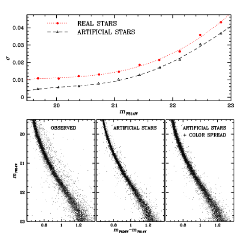
Figure 21: Upper panel: MS dispersion as a function of ${\it m}_{\rm F814W}$ magnitude for NGC 2298. Circles and triangles correspond to real and artificial stars, respectively. The corresponding best fitting $4^{\rm th}$ order polynomials are represented by dotted and dashed lines. Lower panels: comparison of the observed CMD of NGC 2298 (left) and the CMDs of artificial stars before (middle) and after (right) the application of color spread.

In the bottom panels of Fig. 21 we compare the observed CMD of NGC 2298 and the CMDs of artificial stars before and after the application of the color spread. The latter CMD has been used to calculate the ratio between $N_{\rm ART}^{\rm A}$ and $N_{\rm ART}^{\rm B}$ used in Eq. 1.

5 Results

In this Section we illustrate and discuss the main results of this work. Specifically:

• In Sect. 5.1 we analyze the mass-ratio distribution of binaries in each of the 59 GCs studied in this paper in the range 0.5$<q<$1. Results from individual clusters are used to estimate the average mass-ratio distribution of binaries;

• Attempt to calculate the total fraction of MS-MS binaries is proposed in Sect. 5.2;

• Sect. 5.3 gives a summary of the literature measurements of the binary fraction in GCs and compares them with ours.

• In Sect. 5.4 we investigate the distribution of binaries as a function of the primary star mass (magnitude);

• The radial distribution of binaries in each GC is studied in Sect. 5.5;

• Finally, monovariate relations between the binary fraction and the main parent cluster parameters (absolute luminosity, central velocity dispersion, metallicity, age, central density, ellipticity, core and half mass relaxation time, HB morphology, collisional parameter) are discussed in Sect. 5.6.

5.1 Mass-ratio distribution

This section, presents the mass-ratio distribution of the binary population for our target GCs in the range of 0.5$<$q$<$1. To do this, we have divided Region B of the CMD into five intervals of mass ratio (${\it B_{1,2,...,5}}$) as shown in Fig. 22 for NGC 2298. We chose the size of these regions in such a way that each of them covers almost the same area in the portion of the CMD populated by binary systems with $q>0.5$. The sub-region ${\it B_{5}}$ includes also the gray area on the right side of equal-mass binaries fiducial that is populated by binary systems with $q\sim 1$ but large photometric errors.

The fraction of binaries in each sub-region ${\it B_{\rm i}}$ is calculated over the entire WFC field of view following the procedures described in Sect. 4. Each sub-region includes binary stars within a given mass-ratio interval ($\Delta q_{\rm i}$) as labeled in Fig. 22. To account for the different mass-ratio values of each sub-region, and analyze the mass-ratio distribution, we derived the normalized fraction of binaries:

$\nu_{\rm bin,i}=f_{\rm bin,i}/\Delta q_{\rm i}$.

Results for all clusters are shown with black symbols in Figs. 23 and 24. To increase the statistics, we have also divided Region B into two large mass ratio intervals with $0.5<q<0.7$ and $0.7<q<1$ and calculated $\nu_{\rm bin}$ in each of them. The results we obtained by using these $q$ bins are marked with red open circles in Figs. 23 and 24.

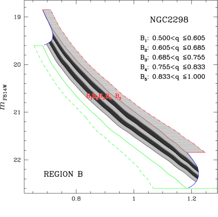
Figure 22: As an example, we show with gray and black shaded areas the five CMD regions (${\it B}_{\rm 1,2,...,5}$) used to determine the mass-ratio distribution of binary stars in NGC 2298.

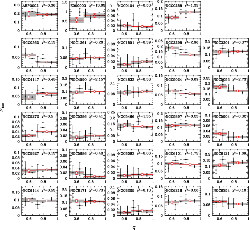
Figure 23: Mass-ratio distribution for the binary population in the ACS field of 29 GCs. Black filled-circles show the normalized fraction of binaries in five mass-ratio intervals, while red open-circles indicate the $\nu_{\rm bin,i}$ values obtained by using only two bins with 0.5$<$q$<$0.7, and 0.7$<$q$<$1. Horizontal segments mark the adopted mass-ratio interval, while observational errors are plotted as the vertical lines and shadowed areas.

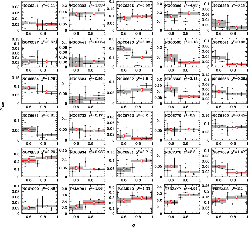
Figure 24: As in Fig. 23 for the remaining 30 GCs.

The mass-ratio distribution is almost flat for most of the GCs of our sample but in few cases we cannot exclude possible deviations from this general trend. To investigate this statement we compared the observations with a flat distribution, calculated for each cluster the reduced $\chi^{2}$ and quoted it in Figs. 23 and 24. Montecarlo simulations demonstrate that in the case of a flat distribution we expect the 50% of the total number of clusters having $\chi^{2}<$1.1 and the 99% $\chi^{2}<$3.8. We found $\chi^{2}$ values higher than 3.8 in four GCs namely NGC 6366 ( $\chi^{2}$=4.92), NGC 6496 ($\chi^{2}$=6.38), TERZAN 7 ( $\chi^{2}$=4.45) and E 3 ($\chi^{2}$=13.62).

To compare the trend of the fraction of binaries as a function of q for different GCs we divided $\nu_{\rm bin,i}$ by two times the fraction of binaries with q$>$0.5 .

Results are in Fig. 25. Black points indicate the measurements for all the GCs, while red points with error bars are the averages in each mass-ratio bin. The gray line is the best fitting line. Its slope is indicated in the figure and suggests that the mass-ratio distribution is nearly flat for q$>$0.5. In the Appendix we will demonstrate that this result is not affected by any significant systematic error.

Since we have determined the mass-ratio distribution over the entire ACS/WFC field of view, our conclusions should indicate the general behavior of the binaries in GCs. Unfortunately, due to the relatively small numbers of binaries, we could not extend this analysis to each sample of ${\it r}_{\rm C}$, the ${\it r}_{\rm C-HM}$, and the ${\it r}_{\rm oHM}$ stars. In these regions, due to mass-segregation effects, the mass-ratio distribution could differ from that shown in Fig. 25.

Up to now, there are few observational constraints on the overall mass-ratio distribution of the binary population in GCs. One of the few measures of f(q) for binary systems, available in the literature, comes from Fisher et al. (2005) who estimated the the mass-ratio distribution function from spectroscopic observations of field binaries within 100 parsecs from the Sun. The f(q) derived by Fisher et al. (2005) is shown in the upper panel of Fig. 26. Binaries with q$<$$\sim$0.9 have a nearly flat distribution while there is a large concentration of binaries formed by two components of similar mass. Tout (1991) studied the binary systems located in the local field and suggests that f(q) can be derived by randomly extracting secondary stars from the observed initial mass function (IMF). The mass-ratio distribution that we obtain by randomly extracting pairs of stars from a Kroupa (2002) IMF is displayed in the upper panel of Fig. 26 for MS binaries with a primary with $0.47<M<0.76M_{\odot}$ which is the typical mass interval corresponding to the magnitude interval we analyzed in the present work. In this case, the f(q) shape rapidly decreases from low to high mass-ratio values with only the 24% of binaries having q$>$0.5.

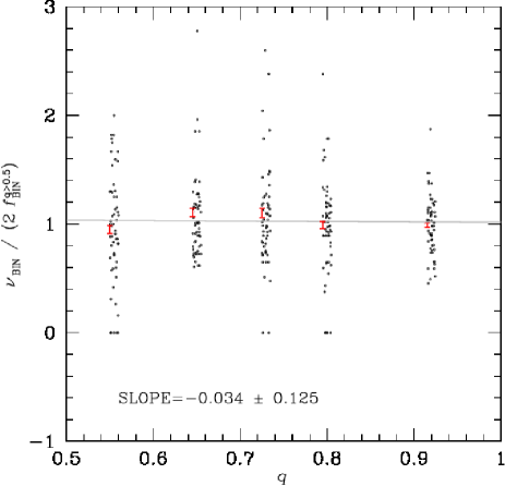
Figure 25: Black points show the normalized fractions of binaries, $\nu_{\rm bin}$ measured in five mass-ratio intervals as a function of q for all the GCs studied in this paper. To compare the fraction of binaries in different clusters we divided $\nu_{\rm bin}$ by two times the fraction of binaries with q$>$0.5. For clarity, black points have been randomly scattered around the corresponding q value. Red points with error bars are the means in each mass-ratio bin, while the gray line is the best fitting line, whose slope is quoted in the inset.

Figure 26: Upper panel: Mass-ratio distribution derived by Fisher et al. (2005). Lower panel: Mass-ratio distribution simulated from random extraction from a Kroupa (2002) IMF in the primary star mass intervals quoted in the inset.

In order to investigate whether the observations of Fig. 25 are consistent with any of the two mass-ratio distributions described above, we calculated the normalized fraction of binaries we expect in the CMD of a GCs where binary stars follow the distribution by Fisher et al. (2005) and the distribution obtained from random extraction of secondary stars from a Kroupa (2002) IMF ($\nu_{\rm bin,F}$, $\nu_{\rm bin,R}$). We also divided each of these quantity by two times the fraction of binaries with q$>$0.5 of the corresponding CMD ($f_{\rm bin,F}^{\rm q>0.5}$, $f_{\rm bin,R}^{\rm q>0.5}$) in close analogy to what done for real stars.

Results are in Fig. 27 where the values of $\nu_{\rm bin,F}/(2\leavevmode\nobreak\ f_{\rm bin,F}^{\rm q>0.5})$ and $\nu_{\rm bin,R}/(2\leavevmode\nobreak\ f_{\rm bin,R}^{\rm q>0.5})$ are plotted as a function of q. The best-fitting least-squares lines are colored gray and their slopes are quoted in the inset. Red points are the observed average binary frequencies of Fig. 25. The large reduced-$\chi$ square values obtained from the comparison of the theoretical and the observed points, and quoted in the figure, indicate that neither the Fisher et al. (2005) nor the Tout (1991) distribution properly matches the distribution we observe in GCs.

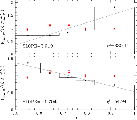
Figure 27: Frequency of binaries divided by two times the fraction of binaries with q$>$0.5 expected for the cases of Fisher et al. (2005) mass-ratio distribution (upper panel) and from the distribution obtained by randomly extracting secondary stars from a Kroupa (2002) IMF (bottom panels). Red points with the error bars are the mean values of the observed binary frequency normalized by two times ${\it f}_{\rm bin}^{\rm q>0.5}$ and have been already plotted in Fig. 25. The slope of the best-fitting least-squares gray straight lines and the reduced-$\chi^{2}$ obtained from the comparison of the observed and theoretical distribution are quoted in the figure.

5.2 The total binary fraction

The procedure described in the previous section allowed us to directly measure the fraction of binaries with q$>$0.5 without any assumptions regarding f(q). On the other hand, because of the photometric errors, binaries with small mass ratios (q$<$0.5) are indistinguishable from single MS stars in this dataset, therefore, any attempt to determine the total fraction of MS-MS binaries without assumption on the mass-ratio distribution is impossible with this approach.

The approach we follow to estimate the total fraction of binaries is similar to that used by Sollima et al. (2007) and consists of assuming a form for f(q). Since none of the two mass-ratio distributions available from literature properly matches the observed distribution in order to estimate the total fraction of binaries ($f_{\rm bin}^{\rm TOT}$), we extrapolated the results of Sect. 5.1 adopting a flat f(q) also for binary systems with q$<$0.5; i. e. , we assumed a constant mass-ratio distribution for all q values. In this case as $f_{\rm bin}^{\rm q>0.5}\equiv f_{\rm bin}^{\rm q<0.5}$ the total fraction of binaries is simply
$f_{\rm bin}^{\rm TOT}=2.0\leavevmode\nobreak\ f_{\rm bin}^{\rm q>0.5}$.
The final $f_{\rm bin}^{\rm TOT}$ are listed in the fifth column of Table 2 for the $r_{\rm C}$, the $r_{\rm C-HM}$, the $r_{\rm oHM}$ sample, and the WFC field.

For completeness, we note that, according to Fisher et al. (2005), 66.5% of binary systems have mass ratio larger than 0.5. Hence, assuming a Fisher et al. (2005) mass ration distribution, the total fraction of binaries should be:
$f_{\rm bin}^{\rm TOT,F}=1.504\leavevmode\nobreak\ f_{\rm bin}^{\rm q>0.5}$.
If we assume that binary stars are formed by random associations between stars of different masses, only 24% of binaries have q$>$0.5, and the total fraction of binaries becomes:
$f_{\rm bin}^{\rm TOT,R}=4.167\leavevmode\nobreak\ f_{\rm bin}^{\rm q>0.5}$.

Table 2: Fraction of binaries with mass ratio $q>0.5$, $q>0.6$ and $q>0.7$, and total fraction of binaries measured for ${\it r}_{\rm C}$, ${\it r}_{\rm C-HM}$, and ${\it r}_{\rm oHM}$ sample and in the whole ACS/WFC field of view for the target GCs. We have analyzed only the ACS/WFC region with radial distance from the cluster center larger than a minimum radius ${\it R}_{\rm min}$ whose value, in arcminutes, is listed in the first column.

ID	REGION	${\it f}_{\rm bin}^{\rm q>0.5}$	${\it f}_{\rm bin}^{\rm q>0.6}$	${\it f}_{\rm bin}^{\rm q>0.7}$	${\it f}_{\rm bin}^{\rm TOT}$
ARP 2	${\it r}_{\rm C}$ sample	0.093$\pm$0.010	0.076$\pm$0.007	0.055$\pm$0.005	0.186$\pm$0.020
	${\it r}_{\rm C-HM}$ sample	0.119$\pm$0.023	0.093$\pm$0.017	0.056$\pm$0.012	0.238$\pm$0.046
	${\it r}_{\rm oHM}$ sample	0.091$\pm$0.031	0.086$\pm$0.024	0.081$\pm$0.017	0.182$\pm$0.062
${\it R}_{\rm min}$=0.00	WFC field	0.096$\pm$0.009	0.079$\pm$0.006	0.057$\pm$0.004	0.192$\pm$0.018
E 3	${\it r}_{\rm C}$ sample	0.360$\pm$0.043	0.350$\pm$0.042	0.247$\pm$0.035	0.720$\pm$0.086
	${\it r}_{\rm C-HM}$ sample	0.317$\pm$0.203	0.147$\pm$0.171	0.264$\pm$0.171	0.634$\pm$0.406
	${\it r}_{\rm oHM}$ sample	0.082$\pm$0.107	0.103$\pm$0.107	0.029$\pm$0.075	0.164$\pm$0.214
${\it R}_{\rm min}$=0.00	WFC field	0.347$\pm$0.041	0.336$\pm$0.039	0.237$\pm$0.033	0.694$\pm$0.082
NGC 104	${\it r}_{\rm C}$ sample	—	—	—	—
	${\it r}_{\rm C-HM}$ sample	0.009$\pm$0.003	0.007$\pm$0.003	0.005$\pm$0.003	0.018$\pm$0.006
	${\it r}_{\rm oHM}$ sample	—	—	—	—
${\it R}_{\rm min}$=0.83	WFC field	0.009$\pm$0.003	0.007$\pm$0.003	0.005$\pm$0.003	0.018$\pm$0.006
NGC 288	${\it r}_{\rm C}$ sample	0.056$\pm$0.005	0.050$\pm$0.004	0.041$\pm$0.003	0.112$\pm$0.010
	${\it r}_{\rm C-HM}$ sample	0.054$\pm$0.007	0.045$\pm$0.005	0.030$\pm$0.004	0.108$\pm$0.014
	${\it r}_{\rm oHM}$ sample	0.092$\pm$0.040	0.032$\pm$0.016	0.021$\pm$0.011	0.184$\pm$0.080
${\it R}_{\rm min}$=0.00	WFC field	0.056$\pm$0.004	0.048$\pm$0.003	0.038$\pm$0.003	0.112$\pm$0.008
NGC 362	${\it r}_{\rm C}$ sample	—	—	—	—
	${\it r}_{\rm C-HM}$ sample	0.025$\pm$0.004	0.018$\pm$0.003	0.010$\pm$0.003	0.050$\pm$0.008
	${\it r}_{\rm oHM}$ sample	0.016$\pm$0.003	0.011$\pm$0.003	0.008$\pm$0.003	0.032$\pm$0.006
${\it R}_{\rm min}$=0.42	WFC field	0.020$\pm$0.003	0.013$\pm$0.003	0.008$\pm$0.003	0.040$\pm$0.006
NGC 1261	${\it r}_{\rm C}$ sample	0.023$\pm$0.009	0.023$\pm$0.006	0.021$\pm$0.005	0.046$\pm$0.018
	${\it r}_{\rm C-HM}$ sample	0.032$\pm$0.004	0.028$\pm$0.003	0.021$\pm$0.003	0.064$\pm$0.008
	${\it r}_{\rm oHM}$ sample	0.020$\pm$0.003	0.018$\pm$0.003	0.012$\pm$0.003	0.040$\pm$0.006
${\it R}_{\rm min}$=0.00	WFC field	0.024$\pm$0.003	0.021$\pm$0.003	0.015$\pm$0.003	0.048$\pm$0.006
NGC 1851	${\it r}_{\rm C}$ sample	—	—	—	—
	${\it r}_{\rm C-HM}$ sample	—	—	—	—
	${\it r}_{\rm oHM}$ sample	0.008$\pm$0.003	0.008$\pm$0.003	0.006$\pm$0.003	0.016$\pm$0.006
${\it R}_{\rm min}$=0.67	WFC field	0.008$\pm$0.003	0.008$\pm$0.003	0.006$\pm$0.003	0.016$\pm$0.006
NGC 2298	${\it r}_{\rm C}$ sample	0.077$\pm$0.009	0.066$\pm$0.006	0.041$\pm$0.004	0.154$\pm$0.018
	${\it r}_{\rm C-HM}$ sample	0.056$\pm$0.007	0.047$\pm$0.005	0.036$\pm$0.004	0.112$\pm$0.014
	${\it r}_{\rm oHM}$ sample	0.047$\pm$0.004	0.034$\pm$0.003	0.023$\pm$0.003	0.094$\pm$0.008
${\it R}_{\rm min}$=0.00	WFC field	0.073$\pm$0.004	0.054$\pm$0.003	0.036$\pm$0.003	0.146$\pm$0.008
NGC 3201	${\it r}_{\rm C}$ sample	0.064$\pm$0.004	0.056$\pm$0.003	0.042$\pm$0.003	0.128$\pm$0.008
	${\it r}_{\rm C-HM}$ sample	0.054$\pm$0.006	0.039$\pm$0.004	0.026$\pm$0.003	0.108$\pm$0.012
	${\it r}_{\rm oHM}$ sample	—	—	—	—
${\it R}_{\rm min}$=0.00	WFC field	0.061$\pm$0.003	0.051$\pm$0.003	0.037$\pm$0.003	0.122$\pm$0.006
NGC 4147	${\it r}_{\rm C}$ sample	0.131$\pm$0.047	0.103$\pm$0.036	0.044$\pm$0.021	0.262$\pm$0.094
	${\it r}_{\rm C-HM}$ sample	0.017$\pm$0.011	0.041$\pm$0.007	0.036$\pm$0.005	0.034$\pm$0.022
	${\it r}_{\rm oHM}$ sample	0.019$\pm$0.006	0.019$\pm$0.003	0.012$\pm$0.003	0.038$\pm$0.012
${\it R}_{\rm min}$=0.00	WFC field	0.029$\pm$0.005	0.027$\pm$0.003	0.020$\pm$0.003	0.058$\pm$0.010
NGC 4590	${\it r}_{\rm C}$ sample	0.057$\pm$0.006	0.054$\pm$0.004	0.040$\pm$0.003	0.114$\pm$0.012
	${\it r}_{\rm C-HM}$ sample	0.040$\pm$0.004	0.037$\pm$0.003	0.023$\pm$0.003	0.080$\pm$0.008
	${\it r}_{\rm oHM}$ sample	0.053$\pm$0.007	0.038$\pm$0.005	0.025$\pm$0.003	0.106$\pm$0.014
${\it R}_{\rm min}$=0.00	WFC field	0.049$\pm$0.003	0.044$\pm$0.003	0.030$\pm$0.003	0.098$\pm$0.006
NGC 4833	${\it r}_{\rm C}$ sample	0.033$\pm$0.004	0.029$\pm$0.003	0.021$\pm$0.003	0.066$\pm$0.008
	${\it r}_{\rm C-HM}$ sample	0.020$\pm$0.003	0.018$\pm$0.003	0.014$\pm$0.003	0.040$\pm$0.006
	${\it r}_{\rm oHM}$ sample	—	—	—	—
${\it R}_{\rm min}$=0.00	WFC field	0.029$\pm$0.003	0.025$\pm$0.003	0.018$\pm$0.003	0.058$\pm$0.006
NGC 5024	${\it r}_{\rm C}$ sample	—	—	—	—
	${\it r}_{\rm C-HM}$ sample	0.028$\pm$0.003	0.021$\pm$0.003	0.014$\pm$0.003	0.056$\pm$0.006
	${\it r}_{\rm oHM}$ sample	0.033$\pm$0.003	0.024$\pm$0.003	0.019$\pm$0.003	0.066$\pm$0.006
${\it R}_{\rm min}$=0.75	WFC field	0.031$\pm$0.003	0.023$\pm$0.003	0.017$\pm$0.003	0.062$\pm$0.006
NGC 5053	${\it r}_{\rm C}$ sample	0.072$\pm$0.005	0.058$\pm$0.004	0.038$\pm$0.003	0.144$\pm$0.010
	${\it r}_{\rm C-HM}$ sample	0.093$\pm$0.020	0.072$\pm$0.013	0.050$\pm$0.010	0.186$\pm$0.040
	${\it r}_{\rm oHM}$ sample	—	—	—	—
${\it R}_{\rm min}$=0.00	WFC field	0.073$\pm$0.005	0.059$\pm$0.004	0.039$\pm$0.003	0.146$\pm$0.010
NGC 5272	${\it r}_{\rm C}$ sample	0.027$\pm$0.007	0.031$\pm$0.004	0.024$\pm$0.003	0.054$\pm$0.014
	${\it r}_{\rm C-HM}$ sample	0.012$\pm$0.003	0.011$\pm$0.003	0.010$\pm$0.003	0.024$\pm$0.006
	${\it r}_{\rm oHM}$ sample	0.019$\pm$0.003	0.015$\pm$0.003	0.012$\pm$0.003	0.038$\pm$0.006
${\it R}_{\rm min}$=0.00	WFC field	0.017$\pm$0.003	0.015$\pm$0.003	0.012$\pm$0.003	0.034$\pm$0.006
NGC 5286	${\it r}_{\rm C}$ sample	—	—	—	—
	${\it r}_{\rm C-HM}$ sample	—	—	—	—
	${\it r}_{\rm oHM}$ sample	0.011$\pm$0.003	0.008$\pm$0.003	0.007$\pm$0.003	0.022$\pm$0.006
${\it R}_{\rm min}$=0.83	WFC field	0.009$\pm$0.003	0.006$\pm$0.003	0.006$\pm$0.003	0.018$\pm$0.006
NGC 5466	${\it r}_{\rm C}$ sample	0.071$\pm$0.004	0.058$\pm$0.003	0.041$\pm$0.003	0.142$\pm$0.008
	${\it r}_{\rm C-HM}$ sample	0.055$\pm$0.008	0.049$\pm$0.006	0.029$\pm$0.004	0.110$\pm$0.016
	${\it r}_{\rm oHM}$ sample	0.016$\pm$0.035	0.022$\pm$0.024	0.009$\pm$0.010	0.032$\pm$0.070
${\it R}_{\rm min}$=0.00	WFC field	0.066$\pm$0.004	0.055$\pm$0.003	0.038$\pm$0.003	0.132$\pm$0.008
NGC 5897	${\it r}_{\rm C}$ sample	0.059$\pm$0.003	0.051$\pm$0.003	0.037$\pm$0.003	0.118$\pm$0.006
	${\it r}_{\rm C-HM}$ sample	0.025$\pm$0.017	0.012$\pm$0.011	0.008$\pm$0.008	0.050$\pm$0.034
	${\it r}_{\rm oHM}$ sample	—	—	—	—
${\it R}_{\rm min}$=0.00	WFC field	0.058$\pm$0.003	0.049$\pm$0.003	0.035$\pm$0.003	0.116$\pm$0.006
NGC 5904	${\it r}_{\rm C}$ sample	—	—	—	—
	${\it r}_{\rm C-HM}$ sample	0.012$\pm$0.003	0.007$\pm$0.003	0.005$\pm$0.003	0.024$\pm$0.006
	${\it r}_{\rm oHM}$ sample	0.006$\pm$0.009	0.003$\pm$0.004	0.005$\pm$0.003	0.012$\pm$0.018
${\it R}_{\rm min}$=0.67	WFC field	0.011$\pm$0.003	0.007$\pm$0.003	0.005$\pm$0.003	0.022$\pm$0.006

Table 2: Cont.

ID	REGION	${\it f}_{\rm bin}^{\rm q>0.5}$	${\it f}_{\rm bin}^{\rm q>0.6}$	${\it f}_{\rm bin}^{\rm q>0.7}$	${\it f}_{\rm bin}^{\rm TOT}$
NGC 5927	${\it r}_{\rm C}$ sample	0.052$\pm$0.009	0.037$\pm$0.007	0.030$\pm$0.006	0.104$\pm$0.018
	${\it r}_{\rm C-HM}$ sample	0.026$\pm$0.003	0.016$\pm$0.003	0.014$\pm$0.003	0.052$\pm$0.006
	${\it r}_{\rm oHM}$ sample	0.006$\pm$0.003	0.006$\pm$0.003	0.004$\pm$0.003	0.012$\pm$0.006
${\it R}_{\rm min}$=0.00	WFC field	0.016$\pm$0.003	0.012$\pm$0.003	0.010$\pm$0.003	0.032$\pm$0.006
NGC 5986	${\it r}_{\rm C}$ sample	—	—	—	—
	${\it r}_{\rm C-HM}$ sample	0.005$\pm$0.004	0.003$\pm$0.003	0.003$\pm$0.003	0.010$\pm$0.008
	${\it r}_{\rm oHM}$ sample	0.006$\pm$0.003	0.003$\pm$0.003	0.001$\pm$0.003	0.012$\pm$0.006
${\it R}_{\rm min}$=0.83	WFC field	0.006$\pm$0.003	0.003$\pm$0.003	0.002$\pm$0.003	0.012$\pm$0.006
NGC 6093	${\it r}_{\rm C}$ sample	—	—	—	—
	${\it r}_{\rm C-HM}$ sample	—	—	—	—
	${\it r}_{\rm oHM}$ sample	0.006$\pm$0.003	0.006$\pm$0.003	0.004$\pm$0.003	0.012$\pm$0.006
${\it R}_{\rm min}$=0.58	WFC field	0.006$\pm$0.003	0.006$\pm$0.003	0.004$\pm$0.003	0.012$\pm$0.006
NGC 6101	${\it r}_{\rm C}$ sample	0.050$\pm$0.004	0.043$\pm$0.003	0.031$\pm$0.003	0.100$\pm$0.008
	${\it r}_{\rm C-HM}$ sample	0.042$\pm$0.004	0.040$\pm$0.003	0.026$\pm$0.003	0.084$\pm$0.008
	${\it r}_{\rm oHM}$ sample	0.054$\pm$0.007	0.039$\pm$0.005	0.021$\pm$0.003	0.108$\pm$0.014
${\it R}_{\rm min}$=0.00	WFC field	0.048$\pm$0.003	0.041$\pm$0.003	0.028$\pm$0.003	0.096$\pm$0.006
NGC 6121	${\it r}_{\rm C}$ sample	0.074$\pm$0.007	0.073$\pm$0.006	0.052$\pm$0.005	0.148$\pm$0.014
	${\it r}_{\rm C-HM}$ sample	0.051$\pm$0.005	0.042$\pm$0.004	0.030$\pm$0.003	0.102$\pm$0.010
	${\it r}_{\rm oHM}$ sample	—	—	—	—
${\it R}_{\rm min}$=0.00	WFC field	0.061$\pm$0.004	0.055$\pm$0.004	0.039$\pm$0.003	0.122$\pm$0.008
NGC 6144	${\it r}_{\rm C}$ sample	0.066$\pm$0.006	0.059$\pm$0.005	0.046$\pm$0.004	0.132$\pm$0.012
	${\it r}_{\rm C-HM}$ sample	0.039$\pm$0.005	0.029$\pm$0.004	0.017$\pm$0.003	0.078$\pm$0.010
	${\it r}_{\rm oHM}$ sample	0.030$\pm$0.007	0.021$\pm$0.005	0.010$\pm$0.004	0.060$\pm$0.014
${\it R}_{\rm min}$=0.00	WFC field	0.048$\pm$0.003	0.040$\pm$0.003	0.028$\pm$0.003	0.096$\pm$0.006
NGC 6171	${\it r}_{\rm C}$ sample	0.093$\pm$0.011	0.071$\pm$0.008	0.052$\pm$0.007	0.186$\pm$0.022
	${\it r}_{\rm C-HM}$ sample	0.046$\pm$0.003	0.035$\pm$0.003	0.027$\pm$0.003	0.092$\pm$0.006
	${\it r}_{\rm oHM}$ sample	—	—	—	—
${\it R}_{\rm min}$=0.00	WFC field	0.054$\pm$0.003	0.042$\pm$0.003	0.032$\pm$0.003	0.108$\pm$0.006
NGC 6205	${\it r}_{\rm C}$ sample	0.005$\pm$0.003	0.010$\pm$0.003	0.007$\pm$0.003	0.010$\pm$0.006
	${\it r}_{\rm C-HM}$ sample	0.006$\pm$0.003	0.004$\pm$0.003	0.004$\pm$0.003	0.012$\pm$0.006
	${\it r}_{\rm oHM}$ sample	0.012$\pm$0.003	0.006$\pm$0.003	0.004$\pm$0.003	0.024$\pm$0.006
${\it R}_{\rm min}$=0.00	WFC field	0.007$\pm$0.003	0.006$\pm$0.003	0.005$\pm$0.003	0.014$\pm$0.006
NGC 6218	${\it r}_{\rm C}$ sample	0.057$\pm$0.005	0.046$\pm$0.004	0.034$\pm$0.004	0.114$\pm$0.010
	${\it r}_{\rm C-HM}$ sample	0.032$\pm$0.003	0.025$\pm$0.003	0.019$\pm$0.003	0.064$\pm$0.006
	${\it r}_{\rm oHM}$ sample	0.011$\pm$0.013	0.007$\pm$0.009	0.004$\pm$0.007	0.022$\pm$0.026
${\it R}_{\rm min}$=0.00	WFC field	0.037$\pm$0.003	0.030$\pm$0.003	0.023$\pm$0.003	0.074$\pm$0.006
NGC 6254	${\it r}_{\rm C}$ sample	0.039$\pm$0.004	0.032$\pm$0.003	0.023$\pm$0.003	0.078$\pm$0.008
	${\it r}_{\rm C-HM}$ sample	0.022$\pm$0.003	0.017$\pm$0.003	0.012$\pm$0.003	0.044$\pm$0.006
	${\it r}_{\rm oHM}$ sample	0.027$\pm$0.007	0.018$\pm$0.005	0.012$\pm$0.003	0.054$\pm$0.014
${\it R}_{\rm min}$=0.00	WFC field	0.029$\pm$0.003	0.023$\pm$0.003	0.016$\pm$0.003	0.058$\pm$0.006
NGC 6341	${\it r}_{\rm C}$ sample	—	—	—	—
	${\it r}_{\rm C-HM}$ sample	0.010$\pm$0.003	0.007$\pm$0.003	0.005$\pm$0.003	0.020$\pm$0.006
	${\it r}_{\rm oHM}$ sample	0.009$\pm$0.003	0.007$\pm$0.003	0.004$\pm$0.003	0.018$\pm$0.006
${\it R}_{\rm min}$=0.42	WFC field	0.011$\pm$0.003	0.008$\pm$0.003	0.006$\pm$0.003	0.022$\pm$0.006
NGC 6352	${\it r}_{\rm C}$ sample	0.092$\pm$0.008	0.078$\pm$0.007	0.054$\pm$0.005	0.184$\pm$0.016
	${\it r}_{\rm C-HM}$ sample	0.053$\pm$0.005	0.041$\pm$0.004	0.034$\pm$0.003	0.106$\pm$0.010
	${\it r}_{\rm oHM}$ sample	0.039$\pm$0.017	0.026$\pm$0.014	0.015$\pm$0.011	0.078$\pm$0.034
${\it R}_{\rm min}$=0.00	WFC field	0.069$\pm$0.004	0.055$\pm$0.003	0.042$\pm$0.003	0.138$\pm$0.008
NGC 6362	${\it r}_{\rm C}$ sample	0.060$\pm$0.004	0.044$\pm$0.003	0.034$\pm$0.003	0.120$\pm$0.008
	${\it r}_{\rm C-HM}$ sample	0.021$\pm$0.005	0.020$\pm$0.004	0.016$\pm$0.003	0.042$\pm$0.010
	${\it r}_{\rm oHM}$ sample	0.032$\pm$0.037	0.023$\pm$0.026	0.043$\pm$0.024	0.064$\pm$0.074
${\it R}_{\rm min}$=0.00	WFC field	0.046$\pm$0.003	0.037$\pm$0.003	0.029$\pm$0.003	0.092$\pm$0.006
NGC 6366	${\it r}_{\rm C}$ sample	0.099$\pm$0.007	0.082$\pm$0.006	0.064$\pm$0.006	0.198$\pm$0.014
	${\it r}_{\rm C-HM}$ sample	0.057$\pm$0.015	0.035$\pm$0.012	0.042$\pm$0.012	0.114$\pm$0.030
	${\it r}_{\rm oHM}$ sample	—	—	—	—
${\it R}_{\rm min}$=0.00	WFC field	0.092$\pm$0.007	0.074$\pm$0.006	0.059$\pm$0.005	0.184$\pm$0.014
NGC 6388	${\it r}_{\rm C}$ sample	—	—	—	—
	${\it r}_{\rm C-HM}$ sample	—	—	—	—
	${\it r}_{\rm oHM}$ sample	0.004$\pm$0.004	0.006$\pm$0.003	0.003$\pm$0.003	0.008$\pm$0.008
${\it R}_{\rm min}$=0.83	WFC field	0.008$\pm$0.004	0.006$\pm$0.003	0.003$\pm$0.003	0.016$\pm$0.008
NGC 6397	${\it r}_{\rm C}$ sample	0.035$\pm$0.018	0.037$\pm$0.015	0.037$\pm$0.013	0.070$\pm$0.036
	${\it r}_{\rm C-HM}$ sample	0.012$\pm$0.003	0.010$\pm$0.003	0.005$\pm$0.003	0.024$\pm$0.006
	${\it r}_{\rm oHM}$ sample	0.014$\pm$0.026	0.005$\pm$0.003	0.002$\pm$0.003	0.028$\pm$0.052
${\it R}_{\rm min}$=0.00	WFC field	0.012$\pm$0.003	0.011$\pm$0.003	0.007$\pm$0.003	0.024$\pm$0.006
NGC 6441	${\it r}_{\rm C}$ sample	—	—	—	—
	${\it r}_{\rm C-HM}$ sample	—	—	—	—
	${\it r}_{\rm oHM}$ sample	0.010$\pm$0.005	0.008$\pm$0.004	0.006$\pm$0.003	0.020$\pm$0.010
${\it R}_{\rm min}$=1.00	WFC field	0.010$\pm$0.005	0.008$\pm$0.004	0.006$\pm$0.003	0.020$\pm$0.010
NGC 6496	${\it r}_{\rm C}$ sample	0.089$\pm$0.006	0.073$\pm$0.005	0.051$\pm$0.004	0.178$\pm$0.012
	${\it r}_{\rm C-HM}$ sample	0.077$\pm$0.008	0.053$\pm$0.007	0.036$\pm$0.006	0.154$\pm$0.016
	${\it r}_{\rm oHM}$ sample	0.046$\pm$0.024	0.021$\pm$0.018	0.015$\pm$0.015	0.092$\pm$0.048
${\it R}_{\rm min}$=0.00	WFC field	0.069$\pm$0.005	0.049$\pm$0.004	0.031$\pm$0.003	0.138$\pm$0.010
NGC 6535	${\it r}_{\rm C}$ sample	0.046$\pm$0.016	0.027$\pm$0.012	0.014$\pm$0.008	0.092$\pm$0.032
	${\it r}_{\rm C-HM}$ sample	0.026$\pm$0.013	0.018$\pm$0.009	0.018$\pm$0.009	0.052$\pm$0.026
	${\it r}_{\rm oHM}$ sample	0.028$\pm$0.010	0.016$\pm$0.007	0.012$\pm$0.006	0.056$\pm$0.020
${\it R}_{\rm min}$=0.00	WFC field	0.033$\pm$0.009	0.021$\pm$0.006	0.014$\pm$0.005	0.066$\pm$0.018

Table 2: Cont.

ID	REGION	${\it f}_{\rm bin}^{\rm q>0.5}$	${\it f}_{\rm bin}^{\rm q>0.6}$	${\it f}_{\rm bin}^{\rm q>0.7}$	${\it f}_{\rm bin}^{\rm TOT}$
NGC 6541	${\it r}_{\rm C}$ sample	—	—	—	—
	${\it r}_{\rm C-HM}$ sample	0.014$\pm$0.003	0.010$\pm$0.003	0.005$\pm$0.003	0.028$\pm$0.006
	${\it r}_{\rm oHM}$ sample	0.010$\pm$0.003	0.005$\pm$0.003	0.001$\pm$0.003	0.020$\pm$0.006
${\it R}_{\rm min}$=0.42	WFC field	0.010$\pm$0.003	0.007$\pm$0.003	0.003$\pm$0.003	0.020$\pm$0.006
NGC 6584	${\it r}_{\rm C}$ sample	0.045$\pm$0.006	0.045$\pm$0.004	0.034$\pm$0.003	0.090$\pm$0.012
	${\it r}_{\rm C-HM}$ sample	0.036$\pm$0.007	0.025$\pm$0.005	0.020$\pm$0.003	0.072$\pm$0.014
	${\it r}_{\rm oHM}$ sample	0.025$\pm$0.003	0.016$\pm$0.003	0.009$\pm$0.003	0.050$\pm$0.006
${\it R}_{\rm min}$=0.00	WFC field	0.039$\pm$0.003	0.030$\pm$0.003	0.021$\pm$0.003	0.078$\pm$0.006
NGC 6624	${\it r}_{\rm C}$ sample	—	—	—	—
	${\it r}_{\rm C-HM}$ sample	0.013$\pm$0.004	0.002$\pm$0.003	0.001$\pm$0.003	0.026$\pm$0.008
	${\it r}_{\rm oHM}$ sample	0.013$\pm$0.005	0.018$\pm$0.005	0.010$\pm$0.004	0.026$\pm$0.010
${\it R}_{\rm min}$=0.42	WFC field	0.011$\pm$0.004	0.012$\pm$0.003	0.007$\pm$0.003	0.022$\pm$0.008
NGC 6637	${\it r}_{\rm C}$ sample	0.062$\pm$0.010	0.060$\pm$0.007	0.057$\pm$0.006	0.124$\pm$0.020
	${\it r}_{\rm C-HM}$ sample	0.029$\pm$0.004	0.028$\pm$0.003	0.020$\pm$0.003	0.058$\pm$0.008
	${\it r}_{\rm oHM}$ sample	0.013$\pm$0.003	0.008$\pm$0.003	0.005$\pm$0.003	0.026$\pm$0.006
${\it R}_{\rm min}$=0.00	WFC field	0.030$\pm$0.003	0.024$\pm$0.003	0.019$\pm$0.003	0.060$\pm$0.006
NGC 6652	${\it r}_{\rm C}$ sample	0.172$\pm$0.055	0.091$\pm$0.038	0.059$\pm$0.029	0.344$\pm$0.110
	${\it r}_{\rm C-HM}$ sample	0.052$\pm$0.006	0.032$\pm$0.004	0.018$\pm$0.003	0.104$\pm$0.012
	${\it r}_{\rm oHM}$ sample	0.027$\pm$0.006	0.021$\pm$0.005	0.016$\pm$0.004	0.054$\pm$0.012
${\it R}_{\rm min}$=0.00	WFC field	0.042$\pm$0.004	0.027$\pm$0.003	0.018$\pm$0.003	0.084$\pm$0.008
NGC 6656	${\it r}_{\rm C}$ sample	0.023$\pm$0.003	0.018$\pm$0.003	0.013$\pm$0.003	0.046$\pm$0.006
	${\it r}_{\rm C-HM}$ sample	0.020$\pm$0.003	0.015$\pm$0.003	0.010$\pm$0.003	0.040$\pm$0.006
	${\it r}_{\rm oHM}$ sample	—	—	—	—
${\it R}_{\rm min}$=0.00	WFC field	0.022$\pm$0.003	0.017$\pm$0.003	0.012$\pm$0.003	0.044$\pm$0.006
NGC 6681	${\it r}_{\rm C}$ sample	—	—	—	—
	${\it r}_{\rm C-HM}$ sample	0.026$\pm$0.005	0.013$\pm$0.003	0.006$\pm$0.003	0.052$\pm$0.010
	${\it r}_{\rm oHM}$ sample	0.005$\pm$0.004	0.011$\pm$0.003	0.010$\pm$0.003	0.010$\pm$0.008
${\it R}_{\rm min}$=0.10	WFC field	0.019$\pm$0.003	0.013$\pm$0.003	0.008$\pm$0.003	0.038$\pm$0.006
NGC 6723	${\it r}_{\rm C}$ sample	0.031$\pm$0.004	0.025$\pm$0.003	0.020$\pm$0.003	0.062$\pm$0.008
	${\it r}_{\rm C-HM}$ sample	0.013$\pm$0.003	0.011$\pm$0.003	0.006$\pm$0.003	0.026$\pm$0.006
	${\it r}_{\rm oHM}$ sample	0.017$\pm$0.004	0.008$\pm$0.003	0.008$\pm$0.003	0.034$\pm$0.008
${\it R}_{\rm min}$=0.00	WFC field	0.023$\pm$0.003	0.017$\pm$0.003	0.013$\pm$0.003	0.046$\pm$0.006
NGC 6752	${\it r}_{\rm C}$ sample	0.017$\pm$0.016	0.011$\pm$0.008	0.006$\pm$0.004	0.034$\pm$0.032
	${\it r}_{\rm C-HM}$ sample	0.005$\pm$0.003	0.004$\pm$0.003	0.002$\pm$0.003	0.009$\pm$0.006
	${\it r}_{\rm oHM}$ sample	—	—	—	—
${\it R}_{\rm min}$=0.00	WFC field	0.005$\pm$0.003	0.004$\pm$0.003	0.002$\pm$0.003	0.010$\pm$0.006
NGC 6779	${\it r}_{\rm C}$ sample	0.050$\pm$0.009	0.050$\pm$0.006	0.038$\pm$0.005	0.100$\pm$0.018
	${\it r}_{\rm C-HM}$ sample	0.028$\pm$0.003	0.022$\pm$0.003	0.017$\pm$0.003	0.056$\pm$0.006
	${\it r}_{\rm oHM}$ sample	0.023$\pm$0.003	0.016$\pm$0.003	0.012$\pm$0.003	0.046$\pm$0.006
${\it R}_{\rm min}$=0.00	WFC field	0.028$\pm$0.003	0.022$\pm$0.003	0.017$\pm$0.003	0.056$\pm$0.006
NGC 6809	${\it r}_{\rm C}$ sample	0.040$\pm$0.003	0.031$\pm$0.003	0.023$\pm$0.003	0.080$\pm$0.006
	${\it r}_{\rm C-HM}$ sample	—	—	—	—
	${\it r}_{\rm oHM}$ sample	—	—	—	—
${\it R}_{\rm min}$=0.00	WFC field	0.040$\pm$0.003	0.031$\pm$0.003	0.023$\pm$0.003	0.080$\pm$0.006
NGC 6838	${\it r}_{\rm C}$ sample	0.152$\pm$0.017	0.120$\pm$0.015	0.080$\pm$0.012	0.304$\pm$0.034
	${\it r}_{\rm C-HM}$ sample	0.110$\pm$0.008	0.100$\pm$0.007	0.072$\pm$0.006	0.220$\pm$0.016
	${\it r}_{\rm oHM}$ sample	0.104$\pm$0.014	0.084$\pm$0.012	0.076$\pm$0.011	0.208$\pm$0.028
${\it R}_{\rm min}$=0.00	WFC field	0.117$\pm$0.007	0.101$\pm$0.006	0.074$\pm$0.005	0.234$\pm$0.014
NGC 6934	${\it r}_{\rm C}$ sample	—	—	—	—
	${\it r}_{\rm C-HM}$ sample	0.032$\pm$0.003	0.027$\pm$0.003	0.017$\pm$0.003	0.064$\pm$0.006
	${\it r}_{\rm oHM}$ sample	0.020$\pm$0.004	0.019$\pm$0.003	0.012$\pm$0.003	0.040$\pm$0.008
${\it R}_{\rm min}$=0.42	WFC field	0.023$\pm$0.003	0.021$\pm$0.003	0.013$\pm$0.003	0.046$\pm$0.006
NGC 6981	${\it r}_{\rm C}$ sample	0.049$\pm$0.009	0.053$\pm$0.006	0.041$\pm$0.005	0.098$\pm$0.018
	${\it r}_{\rm C-HM}$ sample	0.031$\pm$0.008	0.035$\pm$0.006	0.031$\pm$0.004	0.062$\pm$0.016
	${\it r}_{\rm oHM}$ sample	0.034$\pm$0.006	0.028$\pm$0.004	0.019$\pm$0.003	0.068$\pm$0.012
${\it R}_{\rm min}$=0.00	WFC field	0.038$\pm$0.004	0.037$\pm$0.003	0.029$\pm$0.003	0.076$\pm$0.008
NGC 7078	${\it r}_{\rm C}$ sample	—	—	—	—
	${\it r}_{\rm C-HM}$ sample	0.010$\pm$0.005	0.012$\pm$0.003	0.009$\pm$0.003	0.020$\pm$0.010
	${\it r}_{\rm oHM}$ sample	0.018$\pm$0.003	0.014$\pm$0.003	0.007$\pm$0.003	0.036$\pm$0.006
${\it R}_{\rm min}$=0.83	WFC field	0.017$\pm$0.003	0.014$\pm$0.003	0.007$\pm$0.003	0.034$\pm$0.006
NGC 7089	${\it r}_{\rm C}$ sample	—	—	—	—
	${\it r}_{\rm C-HM}$ sample	0.032$\pm$0.006	0.018$\pm$0.004	0.009$\pm$0.003	0.064$\pm$0.012
	${\it r}_{\rm oHM}$ sample	0.011$\pm$0.003	0.009$\pm$0.003	0.005$\pm$0.003	0.022$\pm$0.006
${\it R}_{\rm min}$=0.83	WFC field	0.013$\pm$0.003	0.009$\pm$0.003	0.005$\pm$0.003	0.026$\pm$0.006
NGC 7099	${\it r}_{\rm C}$ sample	0.035$\pm$0.015	0.033$\pm$0.015	0.010$\pm$0.003	0.070$\pm$0.030
	${\it r}_{\rm C-HM}$ sample	0.012$\pm$0.003	0.010$\pm$0.003	0.008$\pm$0.003	0.024$\pm$0.006
	${\it r}_{\rm oHM}$ sample	0.013$\pm$0.003	0.009$\pm$0.003	0.007$\pm$0.003	0.026$\pm$0.006
${\it R}_{\rm min}$=0.00	WFC field	0.012$\pm$0.003	0.010$\pm$0.003	0.008$\pm$0.003	0.024$\pm$0.006
PALOMAR 1	${\it r}_{\rm C}$ sample	0.333$\pm$0.096	0.311$\pm$0.092	0.244$\pm$0.079	0.666$\pm$0.192
	${\it r}_{\rm C-HM}$ sample	0.130$\pm$0.042	0.116$\pm$0.037	0.093$\pm$0.033	0.260$\pm$0.084
	${\it r}_{\rm oHM}$ sample	0.095$\pm$0.031	0.089$\pm$0.027	0.070$\pm$0.023	0.190$\pm$0.062
${\it R}_{\rm min}$=0.00	WFC field	0.146$\pm$0.027	0.136$\pm$0.024	0.108$\pm$0.021	0.292$\pm$0.054
PALOMAR 12	${\it r}_{\rm C}$ sample	0.130$\pm$0.057	0.130$\pm$0.045	0.104$\pm$0.037	0.260$\pm$0.114
	${\it r}_{\rm C-HM}$ sample	0.175$\pm$0.018	0.144$\pm$0.015	0.108$\pm$0.013	0.350$\pm$0.036
	${\it r}_{\rm oHM}$ sample	0.066$\pm$0.019	0.055$\pm$0.014	0.044$\pm$0.012	0.132$\pm$0.038
${\it R}_{\rm min}$=0.00	WFC field	0.137$\pm$0.013	0.114$\pm$0.011	0.087$\pm$0.009	0.274$\pm$0.026
TERZAN 7	${\it r}_{\rm C}$ sample	0.187$\pm$0.017	0.159$\pm$0.013	0.140$\pm$0.011	0.374$\pm$0.034
	${\it r}_{\rm C-HM}$ sample	0.084$\pm$0.016	0.092$\pm$0.013	0.073$\pm$0.010	0.168$\pm$0.032
	${\it r}_{\rm oHM}$ sample	0.088$\pm$0.011	0.075$\pm$0.008	0.051$\pm$0.006	0.176$\pm$0.022
${\it R}_{\rm min}$=0.00	WFC field	0.117$\pm$0.008	0.104$\pm$0.006	0.083$\pm$0.005	0.234$\pm$0.016
TERZAN 8	${\it r}_{\rm C}$ sample	0.083$\pm$0.011	0.072$\pm$0.008	0.056$\pm$0.006	0.166$\pm$0.022
	${\it r}_{\rm C-HM}$ sample	—	—	—	—
	${\it r}_{\rm oHM}$ sample	0.059$\pm$0.009	0.047$\pm$0.006	0.037$\pm$0.005	0.118$\pm$0.018
${\it R}_{\rm min}$=0.00	WFC field	0.067$\pm$0.007	0.056$\pm$0.005	0.044$\pm$0.004	0.134$\pm$0.014

5.3 Comparison with previous measurements of the binary fraction in GCs

To date, the fraction of binaries has been measured for 30 GCs. In Table 3 we list the photometric binary fraction in Galactic GCs from previous measurements and available in the literature. Although for some GCs of our sample the fraction of binaries were already estimated in previous works, caution must be used to compare the results presented in this paper with literature ones. In particular, it should be noted that the inferred values of the total fraction of binaries are tightly related to the assumed f(q). Many authors just determined lower limits to the binary fraction, as they studied binary systems with large q that are clearly separated from single MS stars. Without any indication on the mass-ratio interval analyzed, a quantitative comparison of results with these studies is not possible.

From the comparison between Table 2 and 3 we note that in some cases the fraction of binaries measured in the same cluster region by different authors strongly differs from the results presented here. As an example, in the case of NGC 6752, Rubenstein & Bailyn (1997) estimated an high fraction of binaries in the core ($f_{\rm bin}$=0.27$\pm$0.12), in disagreement with the results presented in this paper ($f_{\rm bin}^{\rm TOT}$=0.03$\pm$0.03) and in Milone et al. (2010) ($f_{\rm bin}^{\rm q>0.5}$=0.03$\pm$0.01). To investigate these different results, Milone et al. (2010) re-examined the Rubenstein & Bailyn (1997) findings first by analyzing the same data with the improved photometric techniques that are now available, and then using the better datasets that have been collected more recently. They concluded that the disagreement comes from the use of the stellar photometry tools they used, which allow a better separation of stellar blends. Similarly, the large fraction of binaries detected by Albrow et al. (2001) in NGC 104, and Fisher et al. (1995) are not confirmed by our study.

Sollima et al. (2007) have recently measured the fraction of binaries in the core of 13 low-density GCs by using the same images studied in this paper. First, they analyzed the color distribution of MS stars to directly derive the minimum fraction of binary systems required to reproduce the observed CMD morphologies, then they inferred two different estimates of the total fraction of binaries by assuming the mass-ratio distribution obtained from random extractions from a de Marchi et al. (2005) IMF, and from the distribution measured by Fisher et al. (2005).

Even if we have shown that the Fisher et al. (2005) distribution is not consistent with what found in the present work and because the images are the same as in this paper, for a meaningful comparison with Sollima et al. (2007), in Fig. 28 we compare the total fraction of binaries in the core that we obtained by assuming the Fisher et al. (2005) distribution (red circles) with the values from Sollima et al. (2007). Blue triangles correspond to the binary fraction estimated in this paper assuming a flat q distribution. For eight out of thirteen GCs, results are in agreement, at the level of less than three $\sigma$. In the cases of ARP 2, NGC 6101, NGC 6723, NGC 6981, and Terzan 7 the fraction of binaries measured in this work is systematically smaller than those found by Sollima and collaborators.

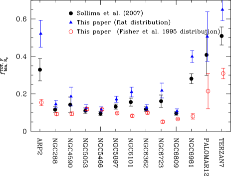
Figure 28: Comparison of the core binary fractions of 13 GCs measured in this paper (red circles) and in Sollima et al. (2007, black circles). In both cases has been assumed the mass-ratio distribution from Fisher et al. (2005). Blue triangles indicate the binary fraction estimated in this work assuming a flat q distribution.

5.4 The binary fraction as a function of primary-star mass

In this Section we investigate the distribution of binary systems as a function of the magnitude. To do this, we calculated the fraction of binaries over the entire WFC/ACS field of view in the three magnitude intervals, containing all the single MS stars and the binary systems with a primary star: [0.75,1.75], [1.75,2.75], [2.75,3.75], F814W magnitudes below the MSTO respectively. In the cases of NGC 6388 and NGC 6441 we used smaller magnitudes intervals of [0.75,1.25], [1.25,1.75], [1.75,2.25] F814W magnitudes below the MSTO. We divided the CMD regions A and B defined in Sect. 4 and illustrated in Fig. 11 into three subregions (named ${\it A}_{\rm b}$, ${\it A}_{\rm i}$, ${\it A}_{\rm f}$ and ${\it B}_{\rm b}$, ${\it B}_{\rm i}$, ${\it B}_{\rm f}$) as shown in Fig. 29 and calculated the fraction of binaries in each magnitude interval see eq. 1.

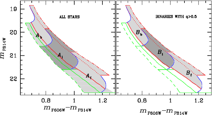
Figure 29: Dark and light gray areas indicate the CMD regions used to measure the fraction of binaries in three magnitude intervals.

Results are shown in Figs. 30 and  31 where we plot the fractions of binaries with mass ratio q$>$0.5 calculated in three magnitude bins as a function of the difference between the mean F814W magnitude of the bin and the F814W magnitude of the MS turn off ($\Delta{\it m}_{\rm F814W}$). Red points indicate the fraction of binaries in the full interval [0.75:3.75] ([0.75:2.15] for NGC 6388 and NGC 6441), while the shadowed area indicates the error associated to this measure.

In general we find no evidence for a significant trend in the fraction of binaries with magnitude (which is a proxy for primary mass), as suggested by the reduced-$\chi^{2}$ values quoted in Figs. 30 and 31. Montecarlo simulations show that in the case of a flat distribution the 50% and 99% of objects have $\chi^{2}$ values smaller than 1.1 and 5.5 respectively. Possible exceptions to this rule of a flat trend are represented by NGC 5897 and NGC 6652 for which we have estimated $\chi^{2}$ values higher than 5.5. And large $\chi^{2}>5.0$ are obtained also for NGC 6144, NGC 6637, and NGC 6723.

In order to further analyze the general trend of the binary fraction with the magnitude for all the GCs studied in this paper we divided the values of ${\it f}_{\rm bin}^{\rm q>0.5}$ measured in each magnitude bin by the fraction of binaries with q$>$0.5 in the interval between 0.75 and 3.75 magnitudes below the MS turn off. Results are shown in Fig. 32 and confirm that the fraction of binaries is nearly flat in the analyzed magnitude range.

Finally, we used isochrones to estimate the average mass of the single stars and the primary component of binary systems in the regions ${\it A}_{\rm b}$, ${\it A}_{\rm i}$, and ${\it A}_{\rm f}$. To do this we converted the mean F814W magnitudes of the single stars contained in each of these regions into masses through the Dotter et al. (2007) mass-luminosity relations. Figure 33 shows the ratio ${\it f}_{\rm bin,b,i,f}^{\rm q>0.5}/{\it f}_{\rm bin}^{\rm q>0.5}$ as a function of the average mass estimated above and suggests that the binary fraction is nearly flat in the analyzed mass interval.

We recall here, that the results presented in this subsection come from the analysis of the binary fractions measured over the entire ACS/WFC field of view. Due to the relatively small numbers of binaries, we did not extended this analysis to each group of ${\it r}_{\rm C}$, the ${\it r}_{\rm C-HM}$, and the ${\it r}_{\rm oHM}$ stars.

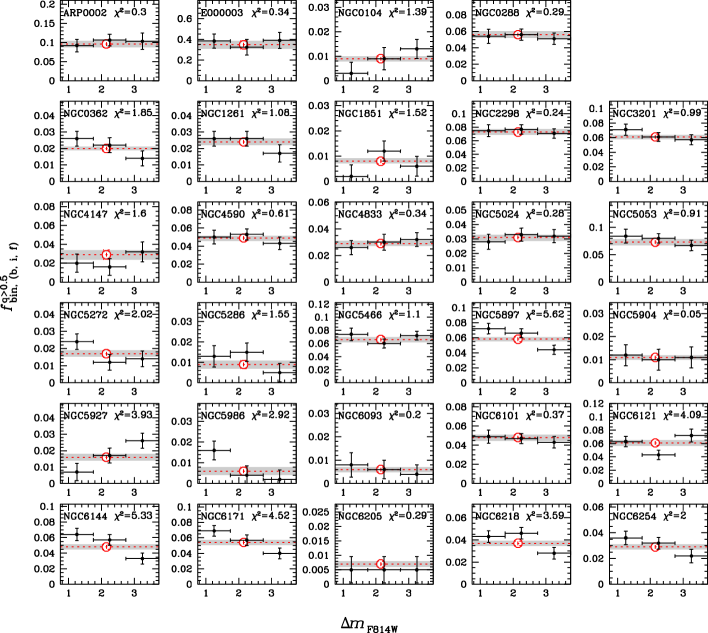
Figure 30: Fraction of binaries with mass ratio q$>$0.5 for 29 GCs measured in three magnitude intervals (black points) and in the interval between 0.75 and 3.75 F814W magnitudes below the MS turn off (red points) as a function of $\Delta{\it m}_{\rm F814W}$. Horizontal segments indicate the magnitude coverage corresponding to each point.

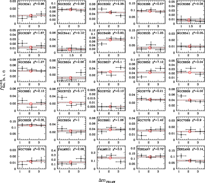
Figure 31: As in Fig. 30 for the remaining 30 GCs. In the cases of NGC 6388 and NGC 6441 the binary fraction has been measured in the interval between 0.75 and 2.25 F814W magnitudes below the MS turn off.

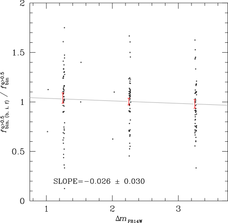
Figure 32: Fraction of binaries with q$>$0.5 measured in three magnitude intervals (black points) as a function of $\Delta{\it m}_{\rm F814W}$ for the 59 GCs studied in this work. To compare the fraction of binaries in different clusters we have divided the fraction of binaries in each bin by the value of ${\it f}_{\rm bin}^{\rm q>0.5}$ measured in the interval between 0.75 and 3.75 F814W magnitudes below the MS turn off. For clarity black points have been randomly scattered around the corresponding $\Delta{\it m}_{\rm F814W}$ value. Red points with error bars are the average binary fractions in each interval while the gray line is the best fitting least-square line whose slope is quoted in the inset.

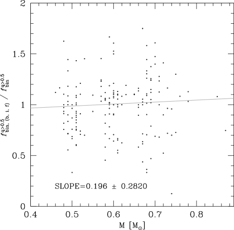
Figure 33: Fraction of binaries with q$>$0.5 measured in three magnitude intervals and normalized by ${\it f}_{\rm bin}^{\rm q>0.5}$ (black points) as a function of the mass of the primary star for the 59 GCs studied in this work.

5.5 The radial distribution

In order to investigate how the fraction of high-mass-ratio binaries depends on the radial distance, we divided the ACS field of view into four concentric annuli, and calculated the fraction of binaries by following the recipes described in Sects. 4 and 5.2. We chose the size of the annulus such that the number of stars that populate the CMD region A is equal in each of them.

Results are shown in Figs. 34 and 35 where we plotted ${\it f}_{\rm bin}^{\rm q>0.5}$ as a function of the explored radial distance for all the GCs studied in this paper.

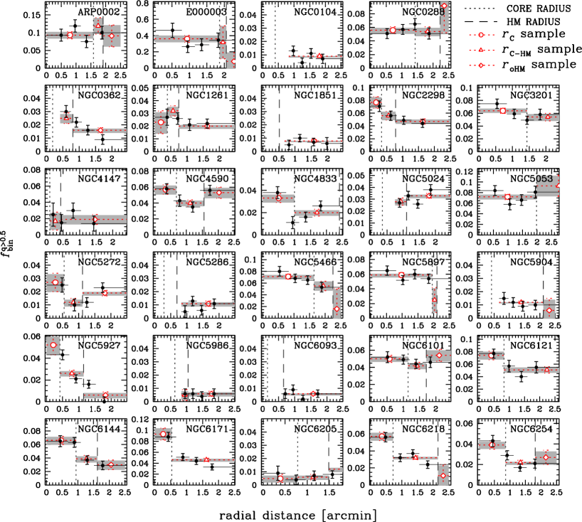
Figure 34: Fraction of binaries with q$>$0.5 as a function of the radial distance from the cluster center for 29 GCs. The dotted and dashed vertical lines mark the core and the half mass radius respectively. Black filled-circles show binary fractions in four radial intervals while red open-symbols indicate the binary fraction for the $r_{\rm C}$, $r_{\rm C-HM}$, and $r_{\rm oHM}$ sample. Horizontal black segments indicate the radial coverage corresponding to each point while observational errors are plotted as vertical lines and shadowed areas.

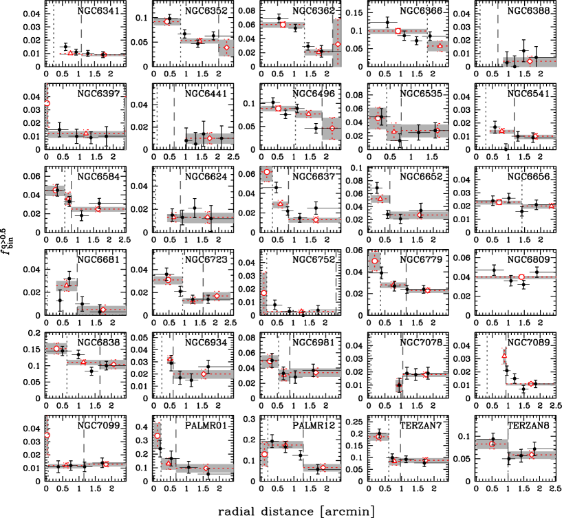
Figure 35: As in Fig. 34 for the remaining GCs.

and confirm that, in most of the GCs where the fraction of binaries has been calculated both in the core and in the outer regions, binaries are significantly more centrally concentrated than single MS stars.

Figure 36: Binary fraction with q$>$0.5 (in units of core binaries) as a function of the distance from the cluster center in units of core radii

In Fig. 36, for the 43 GCs studied in this paper for which we measured the core binary fraction, we plot the fraction of binaries with q$>$0.5 in units of core-binary fraction as a function of the radial distance in units of core radii While it would be naive to assume a similar radial distribution of binaries for all Galactic GCs, it seems clear that the fraction of binaries normalized to the core binary fraction is correlated with radius, and that the binary fraction typically decreases by a factor of $\sim$2 at two core radii with respect to the core binary fraction. The latter behavior was also suggested by Sollima et al. (2007) on the basis of their analysis of the radial distribution of binaries in seven GCs. In the cluster envelope, the binary-fraction trend with radius tends to flatten.

5.6 Correlation between the binary fraction and the parent-cluster parameters

In this section we investigate whether the binary fraction is correlated with any of the physical and morphological parameters of their host GCs. In particular, our analysis makes use of the following quantities:
Relative ages. We used the most recent age measures by Marín-Franch et al. (2009). Relative ages were obtained from the same photometric database used in this paper by comparing the relative position of the clusters’ MS turnoffs, using MS fitting to cross-compare clusters within the sample. Typical errors on the relative age measurements are between 2 % and 7 %. We also used absolute ages from Salaris & Weiss (2002) and De Angeli et al. (2005). Absolute ages are not available for 15 GCs, namely: E3, NGC 4147, NGC 4833, NGC 5024, NGC 5286, NGC 5927, NGC 5986, NGC 6144, NGC 6388, NGC 6441, NGC 6496, NGC 6541, NGC 7089, PAL 1, and TERZAN 8.
Metallicity. We performed our analysis with both the metallicity scales defined by Zinn & West (1984) and Carretta & Gratton  (1997), which were also used by Marín-Franch et al. (2009) to determine relative ages.
BSS Frequency. We used the counts of BSS derived by Moretti et al. (2008) from the WFPC2 photometric catalogs published by Piotto et al. (2002). In particular, we used the normalized number of BSS, which is the absolute number of BSS in a given region divided by the total luminosity coming from the stars in the same region (in unit of 10${}^{4}L_{\odot}$).
Rate of stellar collisions per year.

King, Surdin & Rastorguev (2002) have shown that the rate of stellar collisions per cluster and per year is $\Gamma_{\rm C}=5\times 10^{-15}(\Sigma_{0}^{3}r_{\rm C})^{1/2}$, where $\Sigma_{0}$ is the central surface brightness in units of $L_{\odot,V}pc^{-2}$ and $r_{\rm C}$ is the core radius in units of parsecs. We calculated the probability ($\Gamma_{\rm*}$) that a given star will have a collision in 1 yr, by dividing the collision rate by the total number of stars in the cluster. This is calculated by assuming a mass-luminosity ratio of 2 and a mean mass for colliding stars of 0.4 ${\it M}_{\odot}$.

We also compared the measured fraction of binaries with the encounter frequency adopted by Pooley & Hut (2006) in the approximation used for virialized systems: $\rho_{0}^{1.5}r_{\rm C}^{2}$ where $r_{\rm C}$ is the core radius and $\rho_{0}$ the central stellar density.

The other parameters involved in this analysis are the absolute visual magnitude ${\it M}_{\rm V}$, the ellipticity ($e$), the central concentration ($c$), the core relaxation timescale, $\tau_{\rm c}$, the half-mass relaxation timescale $\tau_{\rm hm}$, and the logarithm of the central luminosity density $\rho_{0}$, and are taken from the Harris (1996) compilation. We also used three different parameters related to the cluster HB morphologies, as discussed in Sect. 5.6.3. Ellipticity ($e$) measurements are not available for six clusters, namely ARP2, E3, NGC 288, PALOMAR 12, Terzan 7 and Terzan 8.

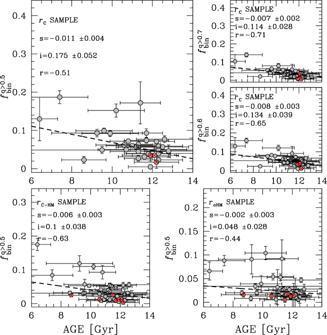
Figure 45: As in Fig. 44 but in this case we used the age measures from Salaris & Weiss (2002) and De Angeli et al. (2005).

Figures 37–47 show the monovariate correlations. Note that, in our study of the core population of binaries, we did not include the post-core-collapse (PCC) GCs, because, for these objects, the definition of core radius is not reliable (Trager et al. 1993). Specifically, PCC clusters are marked with red crosses in these figures but are not used to study the statistical significance of the correlations. Figures 37–47 show that there are no significant correlations between the binary fractions and the cluster ellipticity, core and half mass relaxation time, central concentration and metallicity as suggested by the small values of the Pearson correlation coefficient. Some marginal correlation with the central density can not be excluded.

In the following we will discuss some of the relevant relations between the cluster parameters listed above and the fraction of binaries calculated in three radial regions defined in Sect. 4. A noteworthy correlation of the binary fraction is with the central velocity dispersion (r$\sim$-0.6). as shown in Fig. 37, 38, and  39. The central velocity dispersions $\sigma_{\rm V}$ come from Meylan (1989), and are available only for a subsample of the GCs that are studied in the present work.

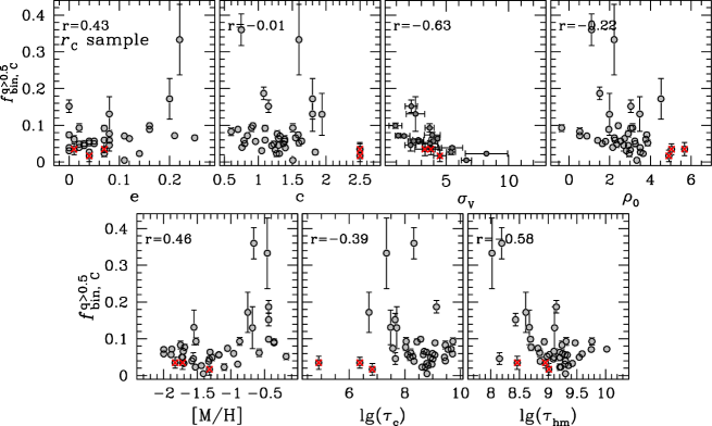
Figure 37: Fraction of binaries with $q>0.5$ in the core as a function of some parameters of their host GCs. Clockwise: ellipticity, central concentration, central velocity dispersion, logarithm of the central luminosity density, half-mass and core relaxation timescale, and metallicity. In each panel we quoted the Pearson correlation coefficient (r). PCC clusters are marked with red crosses and are not used to calculate r (see text for details).

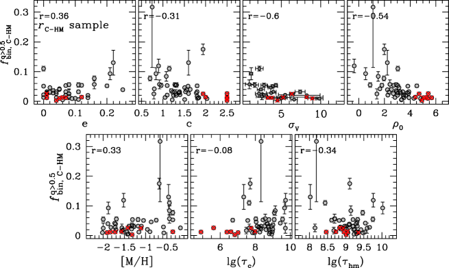
Figure 38: As in Fig. 37 for the ${\it r}_{\rm C-HM}$ sample.

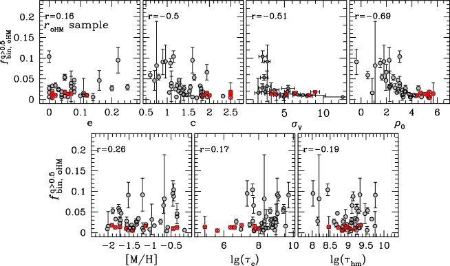
Figure 39: As in Fig. 37 for the ${\it r}_{\rm oHM}$ sample.

5.6.1 ${\it f}_{\rm bin}$ versus ${\it M}_{\rm V}$, $\Gamma_{*}$, and BSS frequency

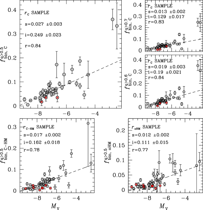
Figure 40: Upper-left: Fraction of binaries with ${\it q}>0.5$ in the core as a function of the absolute visual magnitude of the host GC. Dashed line is the best fitting straight line whose slope (s) and intercept (i) are quoted in the figure together with the Pearson correlation coefficient (r). PCC clusters are marked with red crosses and are not used to calculate neither the best-fitting line nor r. For completeness in the upper-right panels we show the same plot for the fraction of binaries with ${\it q}>0.6$, and ${\it q}>0.7$. Lower panels: Fraction of binaries with ${\it q}>0.5$ in the $r_{\rm C-HM}$ ( left) and $r_{\rm oHM}$ (right) sample as a function of $M_{\rm V}$.

The most significant correlation we found is the correlation between the cluster binary fraction and its absolute magnitude. Clusters with fainter absolute luminosity (smaller mass) have higher binary fractions. This correlation is present in all binary groups, i. e. for binaries inside the cluster core, for binaries located between the core and the half-mass radius, for binaries outside the half-mass radius, and for binaries with q$>$0.5 (Fig. 40). An anticorrelation between the fraction of binaries and the mass of the host GCs is predicted by theoretical models (Sollima 2008, see also Fregeau et al. 2009). These authors suggest that this correlation could be the due to the fact that cluster mass and the efficiency of binary destruction have the same dependence on the cluster density and velocity dispersion.

This anticorrelation might extend to open cluster masses. In fact, Sollima et al. (2010) found a dependence of the fraction of binaries and the cluster mass in a sample of five open clusters. Sollima et al. (2010) suggests that the binary disruption within the cluster core is the dominant process that determine the fraction of binaries in star clusters.

Noteworthy, a similar anticorrelation between the frequency of BSSs and the absolute luminosity of the parent cluster has been found by Piotto et al. (2004), Leigh, Sills, & Knigge (2007), and Moretti et al. (2008). Interestingly enough, Fig. 41 shows that the fraction of binaries is indeed correlated with the fraction of BSSs. Sollima et al. (2008) observed a similar correlation between the BSS specific frequency and the fraction of binaries in the core of 13 low-density Galactic GCs. These authors suggested that the evolution of primordial binaries could be the dominant BSS formation process (see also Knigge et al. 2009 and Leigh, Sills & Knigge 2011). However, Davies et al. (2004) provided a simple model showing that the correlation between the BSS frequency and the cluster mass may be the result of the evolution of the binary fraction due to encounters. Here, we can only note that, figures. 42 and gammacolN seem to suggest a mild correlation between binary fraction and the collisional parameter, while there is no significant correlation between the BSS frequency and the collisional parameter (e. g. Piotto et al. 2004, Davies et al. 2004, Leigh Sills, & Knigge 2007, Moretti et al. 2008). It is clear that the connection between binaries and BSSs is far from trivial. The interpretation of the correlation of binary fraction with cluster parameters, and with BSS fraction is beyond the purposes of the present paper.

Figure 41: Fraction of binaries with ${\it q}>0.5$ as a function of the BSS frequency in the core. PCC GCs are marked with red points.

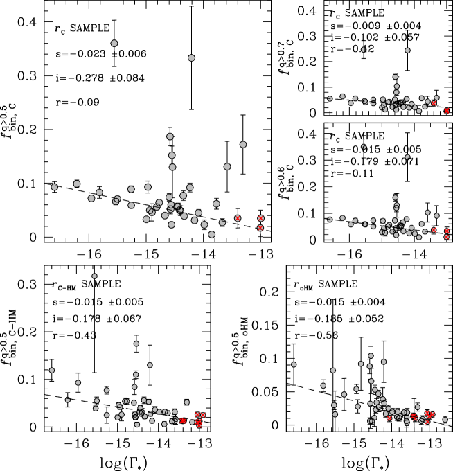
Figure 42: Fraction of binaries with $q>0.5$,$q>0.6$, and $q>0.7$ in the $r_{\rm C}$ region (upper panels) and fraction of binaries with $q>0.5$ in the $r_{\rm C-HM}$ and $r_{\rm oHM}$ regions (bottom panels) as a function of the collisional parameter ($\Gamma_{*}$). The adopted symbols are already defined in Fig. 40.

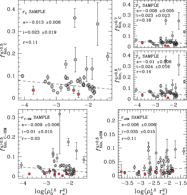
Figure 43: As in Fig. 42. In this case we used the encounter frequency adopted by Pooley & Hut (2006) in the approximation used for virialized systems.

5.6.2 ${\it f}_{\rm bin}$ versus age

Figures 44 and  45 plot the fraction of binaries with ${\it q}>0.5$ in the core as a function of relative ages by Marín-Franch et al. (2009) and the absolute ages from and from Salaris & Weiss  (2002) and De Angeli et al. (2005) respectively. There is no evident trend between ages and the binary fraction.

Sollima et al. (2007) compared the fraction of binaries measured in the core of thirteen clusters, with the cluster ages from Salaris & Weiss (2002) and De Angeli et al. (2005) and found an anticorrelation between age and binary fraction suggesting age as the dominant parameter that determines the fraction of binaries in a GC. Our sample of 59 GCs does not confirm such correlation. Sollima et al. (2007) sample is limited to low density clusters. In order to verify whether the binary fraction dependence on age is limited to low density clusters, in Fig. 46 we plot the binary fraction for the $r_{\rm C}$ sample as a function of the age from De Angeli et al. (2005) and the relative age from Marin Franch et al. (2009) for clusters with central density log$(\rho_{0})<2.75$ (same central density limit of Sollima et al. 2007 sample). We also note that the youngest low density clusters in our sample have a larger binary fraction, but the fact that at least one old GCs (E3) hosts a large binary fraction suggests that more data are needed to confirm any systematic trend.

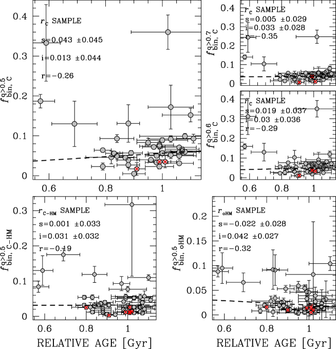
Figure 44: Fraction of binaries with q$>$ 0.5, q$>$0.6, and q$>$0.7 in the $r_{\rm C}$ region (upper panels) and fraction of binaries with q$>$0.5 in the $r_{\rm C-HM}$ and $r_{\rm oHM}$ regions (bottom panels) as a function of the relative age measured by Marín-Franch et al. (2009). The adopted symbols are already defined in Fig. 40.

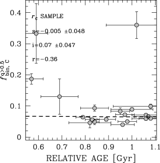
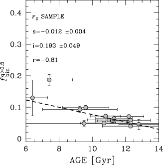
Figure 46: Fraction of binaries with q$>$ 0.5 in the $r_{\rm C}$ sample for low density clusters (log$(\rho_{0})<2.75$) as a function of the relative age from Marín-Franch et al. (2009) (left panel) an absolute age from Salaris & Weiss (2002) and De Angeli et al. (2005) (right panel).

5.6.3 HB morphology

Binaries have been considered as a possible second parameter of the HB morphology by several authors. In particular, the existence of a link between field B-type subdwarf (sdB) – which are the counterpart in the field of the extremely hot horizontal branch (EHB) stars in GCs – and binary systems is well-established, both on observational and theoretical grounds. A large population of binaries has been found among field sdBs (e. g. Napiwotzki et al. 2004 and references therein). However, the formation scenario of EHB stars in GCs may be different. In fact, several radial-velocity surveys for the measurement of the binary fraction among EHB stars have revealed a significant lack of binary systems (Moni Bidin et al. 2006, 2009).

In order to investigate possible relations between the fraction of binaries and the HB shape we used three different parameters:
1) the median color difference between the HB and the RGB [$\Delta(V-I)$], measured by Dotter et al. (2010) for 60 GCs using the same CMDs of this paper;
2) The HB morphology index from Mackey & van den Bergh (2005);
3) the effective temperature of the hottest HB stars ($T_{\rm eff,HB}$), measured by Recio-Blanco et al. (2006). $\Delta(V-I)$, HB index, and $T_{\rm eff,HB}$ measures are available for 56, 55, and 28 GCs studied in this paper.

Monovariate relation between the fraction of binaries with $q>0.5$ and these parameters are shown in Fig. 47. We find no significant relations between the fraction of binaries and the HB parameters, confirming the small or null impact of the binary population on the HB morphology. Similar results are obtained for binaries with $q>0.6$ and $q>0.7$.

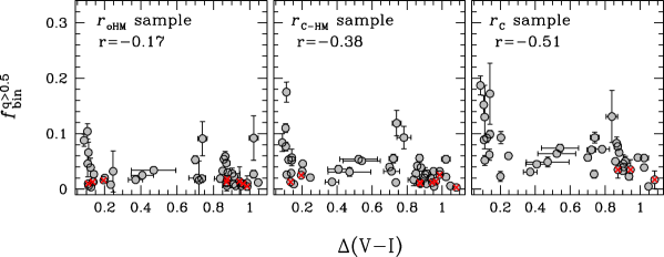
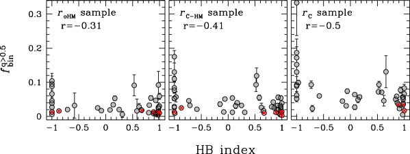
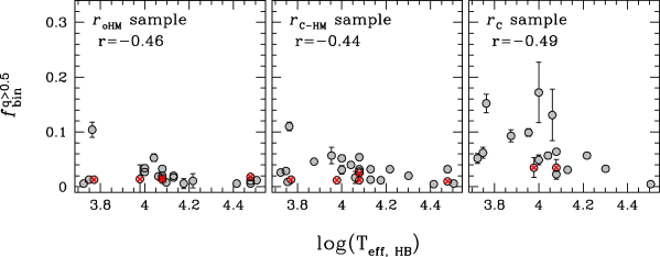
Figure 47: Fraction of binaries with q$>$ 0.5 as a function of the temperature of the hottest HB stars (bottom), the HB morphology index (middle), and the median color difference between the HB and the RGB (top).

ID	${\it f}_{\rm bin}$	note	region	reference
E 3	0.29$\pm$0.09	lower limit	within 2 core radius	Veronesi et al. (1996)
ARP 2	$>$0.08	lower limit	within core	Sollima et al. (2007)
	0.329-0.521	all	within core	Sollima et al. (2007)
NGC 104 (47 Tucanae)	0.14$\pm$0.04	all	within half-mass radius	Albrow et al. (2001)
	$>$0.05	lower limit	outside half-mass radius	De Marchi & Paresce  (1995)
	$\sim$0.02	all	outside half-mass radius	Anderson  (1997)
NGC 288	$>$0.10	lower limit	1-6 core radius	Bolte  (1992)
	0.10-0.20	all	within half-mass radius	Bellazzini et al. (2002)
	0.01${}^{+0.1}_{-0.0}$	all	outside half-mass radiu	Bellazzini et al. (2002)
	$>$0.06	lower limit	within core	Sollima et al. (2007)
	0.116-0.145	all	within core	Sollima et al. (2007)
NGC 362	0.21$\pm$0.06	all	within half-mass radius	Fischer et al. (1993)
NGC 2808	0.20$\pm$0.04		outside half-mass radius	Alcaino et al. (1998)
	0.04$\pm$0.01	all	outside half-mass radius	Milone et al. (2010)
NGC 3201	$<$0.10	upper limit	outside half-mass radius	Cote et al. (2007)
NGC 4590	$>$0.09	lower limit	within core	Sollima et al. (2007)
	0.142-0.186	all	within core	Sollima et al. (2007)
NGC 5053	$>$0.08	lower limit	within core	Sollima et al. (2007)
	0.110-0.125	all	within core	Sollima et al. (2007)
NGC 5139 ($\omega$ Centauri)	$<$0.05	upper limit	outside half-mass radius	Elson et al. (1995)
NGC 5272 (M3)	‘low’	all	outside half-mass radius	Gunn & Griffin  (1979)
	$\sim$0.04	all	outside half-mass radius	Pryor et al. (1988)
	0.14$\pm$0.08	all	inside half-mass radius	Zhao & Bailyn (2005)
	0.02${}^{+0.16}_{-0.02}$	all	outside half-mass radius	Zhao & Bailyn (2005)
NGC 5466	$>$0.08	lower limit	within core	Sollima et al. (2007)
	0.095-0.117	all	within core	Sollima et al. (2007)
NGC 5897	$>$0.07	lower limit	within core	Sollima et al. (2007)
	0.132-0.171	all	within core	Sollima et al. (2007)
NGC 6101	$>$0.09	lower limit	within core	Sollima et al. (2007)
	0.156-0.210	all	within core	Sollima et al. (2007)
NGC 6121 (M4)	$0.23^{+0.34}_{-0.23}$	all	inside half-mass radius	Cote & Fischer (1996)
	$\sim$0.02	all	outside half-mass radius	Richer et al. (2004)
NGC 6341 (M92)	$0.00^{+0.03}_{-0.00}$	lower limit	outside half-mass radius	Anderson  (1997)
NGC 6362	$>$0.06	lower limit	within core	Sollima et al. (2007)
	0.118-0.127	all	within core	Sollima et al. (2007)
NGC 6397	$<$0.07	upper limit	within half-mass radius	Cool & Bolton (2002)
	0.051$\pm$0.010	all	within half-mass radius	Davis et al. (2008)
	0.012$\pm$0.004	all	1.3-2.8 half-mass radii	Davis et al. (2008)
NGC 6656 (M22)	$0.03^{+0.16}_{-0.03}$	all	outside half-mass radius	Cote et al. (1996)
NGC 6723	$>$0.06	lower limit	within core	Sollima et al. (2007)
	0.161-0.218	all	within core	Sollima et al. (2007)
NGC 6752	0.27$\pm$0.12	all	within core	Rubenstein & Bailyn (1997)
	0.03$\pm$0.01	lower limit, q$>$0.5	within core	Milone et al. (2010)
	0.02${}^{+0.16}_{-0.02}$	all	between core and half-mass radius	Rubenstein & Bailyn (1997)
	0.01$\pm$0.01	lower limit, q$>$0.5	between core and half-mass radius	Milone et al. (2010)
NGC 6792	‘low’	all	outside half-mass radius	Catelan et al. (2008)
NGC 6809 (M55)	$>$0.06	lower limit	within core	Sollima et al. (2007)
	0.096-0.108	all	within core	Sollima et al. (2007)
NGC 6838 (M71)	0.22${}^{+0.26}_{-0.12}$	all	within half-mass radius	Yan & Mateo (1994)
NGC 6981	$>$0.10	lower limit	within core	Sollima et al. (2007)
	0.281-0.399	all	within core	Sollima et al. (2007)
NGC 7078 (M15)	$\sim$0.07	all	within half-mass radius	Gebhardt et al. (1994)
NGC 7099 (M30)	$<$0.05	upper limit	outside half-mass radius	Alcaino et al. (1998)
PALOMAR 12	$>$0.18	lower limit	within core	Sollima et al. (2007)
	0.408-0.506	all	within core	Sollima et al. (2007)
PALOMAR 13	$>$0.30$\pm$0.04	lower limit	inside $\sim$18 core radii	Clark et al.  (2004)
TERZAN 7	$>$0.21	lower limit	within core	Sollima et al. (2007)
	0.509-0.649	all	within core	Sollima et al. (2007)

Table 3: Collection of literature binary fraction estimates. For each GC we listed the measured fraction of binaries ($f_{\rm bin}$), specified if the latter is a lower limit, an upper limit or a measure of the total fraction of binaries. We also indicate the spatial region where this measure was done and give the reference.

6 Summary

In this paper we have analyzed the properties of the population of MS binaries of a sample of 59 GCs. The main dataset consists in the ACS/WFC images of the Globular Clusters Treasury project (GO10775, PI Sarajedini) that allowed us to obtain uniform and deep photometry for an unprecedented number of GCs (see Sarajedini et al. 2007 and Anderson et al. 2008 for details). We have also used ACS/WFC, WFC3 and WFPC2 data from the archive to obtain proper motions when images overlapping the GO10775 data are available. The CMDs have been corrected for the effects of differential reddening and photometric zero point variations due to small inaccuracies in the PSF model.

We have measured the fraction of binaries with mass ratio q$>$0.5 and estimated the total fraction of binaries for MS stars that are between 0.75 and 3.75 magnitudes fainter than the MS turn off. We have found that:

• in nearly all the GCs the fraction of binaries is significantly smaller than in the field, where the binary fraction is larger than 0.5 (e. g. Duquennoy et al. 1991, Fisher & Marcy 1992) with a few relevant exceptions (E3, Palomar 1) where the total binary fraction is greater than $\sim$0.4.

• We have obtained the fraction of binaries in five intervals of q (for q$>$0.5) and found that the mass-ratio distribution is generally flat.

• There is no evidence for a significant correlation of the binary fraction with primary mass of the binary system.

• We measured the fraction of binaries in the cluster core, in the region between the core and the half-mass radius, and outside the half-mass radius and studied their radial distribution. Binary stars are more centrally concentrated than single MS stars with the fraction of binaries generally decreasing by a factor of $\sim$2 from the center to about two core radii.

• We investigated monovariate relations between the fraction of binaries (in the ${\it r}_{\rm C}$, ${\it r}_{\rm C-HM}$, and ${\it r}_{\rm oHM}$ sample) and the main parameters of their host GCs (absolute magnitude, HB morphology, age, ellipticity, metallicity, collisional parameter, half mass and core relaxation time, central concentration, central velocity dispersion, and central luminosity density).

• We found a significant anticorrelation between the fraction of binaries in a GC and its absolute luminosity (mass).

• We found a marginal correlation between the cluster central density and the central velocity dispersion.

• We did not find any significant relation between the binary fraction and the HB morphological parameters.

• We confirm a significant correlation between the fraction of binaries and the fraction of BSSs, indicating that the main formation mechanism of BSSs must be related to binary evolution.

APPENDIX A. Reliability of the measured binary fraction.
In this appendix we investigate whether the fraction of binaries with q$>$0.5 that we measured with the procedure described in Sect. 4 are reliable or are affected by any systematic uncertainty due to the method we used. The basic idea of this test consists of simulating a number of CMDs with a given fraction of binaries, measuring the fraction of binaries in each of them, and comparing the added fraction of binaries with the measured ones.
Simulation of the CMD.
We started by using artificial stars to simulate a CMD made of single stars following the procedure already described in Sect. 4.2. To simulate binary stars to be added to the simulated CMD we adopted the following procedure:

• We selected a fraction $f_{\rm bin}^{\rm TOT}$ of single stars equal to the fraction of binaries that we want to add to the CMD and derived their masses by using the Dotter et al. (2007) mass-luminosity relation. In our simulations we assumed the values of $f_{\rm bin}^{\rm TOT}=$0.05, 0.10, 0.30, and 0.50.

• For each of them, we calculated the mass $\mathcal{M}_{2}=q\times\mathcal{M}_{1}$ of the secondary star and obtained the corresponding $m_{\rm F814W}$ magnitude. Its color was derived by the MSRL. For simplicity we assumed a flat mass-ratio distribution.

• Finally, we summed up the F606W and F814W fluxes of the two components, calculated the corresponding magnitudes, added the corresponding photometric error, and replaced the original star in the CMD with this binary system.

As an example, in the upper panels of Fig. 48 we show the artificial star CMD made of single stars only (left panel), and the CMD where we added a fraction $f_{\rm bin}^{\rm TOT}$=0.10 of binaries (right panel), for the case of NGC 2298.

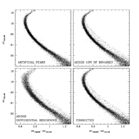
Figure 48: Artificial stars CMD for NGC 2298 (upper-left) and simulated CMD with a fraction of $f_{\rm bin}^{\rm TOT}$0.10 of binaries added (upper-right). Bottom panels show the simulated CMD after we added differential reddening (left) and the simulated CMD after the correction for differential reddening (right).

Simulation of the differential reddening.
To probe how well the reddening correction works, we considered a simple model. The simulation of the differential reddening suffered by any single star is far from trivial as we have poor information on the structure of the interstellar medium between us and each GC. For simplicity, in this work we assumed that reddening variations are related to the positions (X, Y) of each stars by the following relations:

$\Delta E(B-V)=C_{1}(cos(X^{\prime})+sin(Y^{\prime}))$
where
$X^{\prime}=C_{2}\pi(X-X_{\rm MAX})/(X_{\rm MAX}-X_{\rm MIN})$,
$Y^{\prime}=C_{2}\pi(Y-Y_{\rm MAX})/(Y_{\rm MAX}-Y_{\rm MIN})$.
Here $X_{\rm MIN,MAX}$ and $Y_{\rm MIN,MAX}$ are the minimum and the maximum values of the coordinates X and Y, $C_{1}$ is a free parameter that determines the maximum amplitude $E(B-V)$ variation, and $C_{2}$ governs the number of differential reddening peaks within the field of view. In this work, we used for each GC the value of $C_{1}$ that ranges from 0.005 to 0.05 to account for the observed reddening variation in all the GCs, while we arbitrarily assumed three values of $C_{2}$=3, 5, and 8 to reproduce three different fine-scales of differential reddening. As an example, in Fig. 49 we show the map of differential reddening added to the simulated CMD of NGC 2298 that is obtained by assuming $C_{1}=0.025$ and $C_{2}=5$.

Then, we have transformed the values of $\Delta$E(B-V) corresponding to the position of each stars into $\Delta A_{\rm F606W}$, and $\Delta A_{\rm F814W}$ and added these absorption variations to the F606W and the F814W magnitudes. The CMD obtained after we added differential reddening is shown in the bottom left panel of Fig. 48 for NGC 2298. We applied to this simulated CMD the procedure to correct for differential reddening described in Sect. 3.1 and obtain the corrected CMD shown in the bottom right panel. For each of these binary-enhanced simulated CMD, we also generated a CMD made of artificial stars by following the approach described in Sect. 4.2. In our investigation we did not account for field stars. For each combination of the $f_{\rm bin}^{\rm TOT}$ and $C_{2}$ we have simulated 200 CMDs with random values of the $C_{1}$.

Measurements of the binary fraction.
Finally, we used the procedure of Sect. 4 to measure the fraction of binaries with mass ratio q$>$0.5 defined as:
$f_{\rm bin}^{\rm q>0.5}=\frac{N_{\rm SIMU}^{\rm B}}{N_{\rm SIMU}^{\rm A}}-\frac{N_{\rm ART}^{\rm B}}{N_{\rm ART}^{\rm A}}$
where $N_{\rm SIMU}^{\rm A}$ and $N_{\rm SIMU}^{\rm B}$ are the numbers of stars in the regions A and B in the CMD, as defined in Fig. 11 in the binary-enhanced simulated CMD and $N_{\rm ART}^{\rm A}$ and $N_{\rm ART}^{\rm B}$ the numbers of stars in the same regions of the artificial stars CMD.

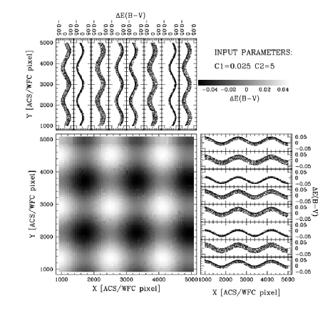
Figure 49: Bottom-left: Map of differential reddening added to the simulated CMD of NGC 2298. The gray levels indicate the reddening variations as indicated in the upper-right panel. Upper-left and bottom-right panels show $\Delta E(B-V)$ as a function of the Y and X coordinate respectively for stars into 8 vertical and horizontal slices.

Results are shown in Fig. 50 where we plotted the difference between the measured and the input fraction of binaries versus the parameter $C_{1}$ for four difference values of the input binary fraction. We found that, for input binary fraction of 0.05, 0.10 and 0.30, the average difference are negligible ($<0.5\%$), as indicated by the the black lines and the numbers quoted in the inset. In the case of a large binary fraction ($f_{\rm bin}^{\rm TOT}$=0.5) the measured fraction of binaries with q$>$0.5 is systematically underestimated by $\sim$0.03. Apparently our results do not depend on the value of the parameter $C_{2}$. Simulations with $C_{2}=$3, 5, and 8 ( indicated in Fig. 50 with red circles, gray triangles, and black crosses, respectively) give indeed the same average differences. Our comparison between the fraction of binaries added to the simulated CMD and the measured ones demonstrate that the fraction of binaries determined in this work and listed in Table 2 are not affected by any significant systematic errors related to the procedure we adopted.

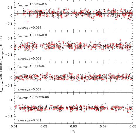
Figure 50: Difference between the measured fraction of binaries and the fraction of binaries in input as a function of the parameter $C_{1}$ for four difference values of the input binary fraction. Black lines indicate the average difference. Red circles, gray triangles and black crosses indicate simulations with $C_{2}=$3, 5, and 8 respectively.

We have also determined the fraction of binaries in five mass-ratio intervals by following the approach described in Sect. 5.1 for real stars. To this aim, we have divided the region B of the CMD defined in Sect. 11 into five subregions as illustrated in Fig. 22 for real stars. The size of each region is chosen in such a way that each of them covers a portion of the CMD with almost the same area. The resulting mass-ratio distribution is shown in Fig. 51, where we have plotted the fraction of binaries per unit q as a function of the mass ratio. As already done in the case of real stars, to compare the mass-ratio distribution in simulated CMDs with different binary fraction, we have divided $\nu_{\rm bin}$ by two times the measured fraction of binaries with q$>$0.5. The best fitting gray line closely reproduce the flat mass-ratio distribution in input with $\nu_{\rm bin}$=1.

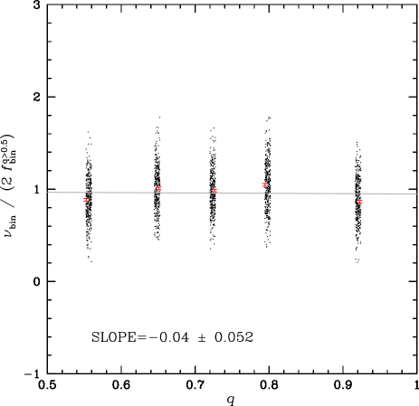
Figure 51: Fractions of binaries per unit q measured in five mass-ratio intervals as a function of q for all the simulated GCs. To compare the q distribution in simulated clusters with different fraction of binaries, we divided $\nu_{\rm bin}$ by two times the fraction of binaries with q$>$0.5. For clarity, black points have been randomly scattered around the corresponding q value. The means normalized binary fractions in each mass-ratio bin are represented by red points with error bars, while the gray line is the best fitting line, whose slope is quoted in the inset.

Finally we have measured in the simulated CMDs the fraction of binaries with ${\it q}>0.5$ in three intervals [0.75,1.75], [1.75,2.75], and [2.75,3.75] F814W magnitudes below the MSTO. To do this we used the procedure already described in Sect. 5.4 for real stars and we have normalized the ${\it f}^{\rm q>0.5}_{\rm bin}$ value measured in each magnitude bin by the fraction of binaries with ${\it q}>0.5$ measured in the whole interval between 0.75 and 3.75 F814W magnitudes below the MSTO. Results are shown in Fig. 52 where we have plotted the normalized binary fractions as a function of $\Delta{\it m}_{\rm F814W}$. The best-fitting gray line is nearly flat, and well reproduces the input magnitude distribution.

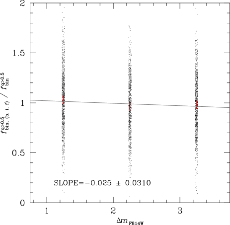
Figure 52: Fraction of binaries with q$>$0.5 in three magnitude intervals as a function of $\Delta{\it m}_{\rm F814W}$ for all the simulated GCs. To compare the measured fraction of binaries in different clusters we have divided the measured binary fractions in each magnitude interval by the value of ${\it f}^{\rm q>0.5}_{\rm bin}$ measured in the interval between 0.75 and 3.75 F814W magnitudes below the MS turn off. Red points with error bars are the means normalized binary fractions in each magnitude interval. The gray line with the quoted slope is the best-fitting least-squares line.

These tests demonstrate that both the mass-ratio distribution determined in Sect. 5.1 for the 59 GCs studied in this work and shown in Fig. 25 as well as the binary fractions measured in different magnitude intervals in Sect. 5.4 are not biased by significant systematic errors related to the procedure we adopted.

References

- Albrow et al. (2001) Albrow, M. D., Gilliland, R. L., Brown, T. M., Edmonds, P. D., Guhathakurta, P., & Sarajedini, A. 2001, ApJ, 559, 1060
- (2) Alcaino, G., Liller, W., Alvarado, F., Kravtsov, V., Ipatov, A., Samus, N., & Smirnov, O. 1998, AJ, 115, 1492
- Anderson (1997) Anderson, J. 1997, PhD thesis, Univ. of California, Berkley
- Anderson (1999) Anderson, J., & King, I. R. 1999, PASP, 111, 1095
- Anderson (2000) Anderson, J., & King, I. R. 2000, PASP, 112, 1360
- Anderson (2003) Anderson, J., & King, I. R. 2003, PASP, 115, 113
- Anderson (2006) Anderson, J., & King, I. R. 2006, ACS Instrument Science Report 2006-01 (Baltimore: STScI)
- Anderson (2008) Anderson, J. et al. 2008, AJ, 135, 2055 paper IV
- Anderson et al. (2009) Anderson, J., Piotto, G., King, I. R., Bedin, L. R., & Guhathakurta, P. 2009, ApJ, 697, L62
- Anderson & van der Marel (2010) Anderson, J., & van der Marel, R. P. 2010, ApJ, 710, 1032
- Aparicio et al. (1990) Aparicio, A., Bertelli, G., Chiosi, C., & Garcia-Pelayo, J. M. 1990, A&A, 240, 262
- Aparicio et al. (1991) Aparicio, A., Bertelli, G., Chiosi, C., & Garcia-Pelayo, J. M. 1991, A&AS, 88, 155
- (13) Bedin, L. R., Cassisi, S., Castelli, F., Piotto, G., Anderson, J., Salaris, M., Momany, Y. & Pietrinferni, A., 2005, MNRAS, 357, 1048
- Bedin et al. (2008) Bedin, L. R., Salaris, M., Piotto, G., Cassisi, S., Milone, A. P., Anderson, J., & King, I. R. 2008, ApJ, 679, L29
- Bellazzini (2002) Bellazzini, M., Fusi Pecci, F., Messineo, M., Monaco, L., Rood, R. T., 2002, AJ, 123, 509 bibitem[Bellini & Bedin(2009)]2009PASP..121.1419B Bellini, A., & Bedin, L. R. 2009, PASP, 121, 1419
- Bellini et al. (2010) Bellini, A., Bedin, L. R., Piotto, G., Milone, A. P., Marino, A. F., & Villanova, S. 2010, AJ140, 631
- Bolte (1992) Bolte, C. D., 1992 ApJS8, 145
- Carretta & Gratton (1997) Carretta, E., & Gratton, R. G. 1997, A&AS, 121, 95
- Catelan et al. (2008) Catelan, M., et al. 2008, Hot Subdwarf Stars and Related Objects, 392, 347
- Clark (2004) Clark, L. L., Sandquist, E. L., Bolte, M., 2004, AJ, 138, 3019
- Cool (2002) Cool, A. M., Bolton, A. S., 2002, in ”Stellar Collisions, Mergers and their Consequences”, M. M. Shara eds., San Francisco ASP Conf. Ser., 263, 163
- Cote et al. (1994) Cote, P., Welch, D. L., Fischer, P., Da Costa, G. S., Tamblyn, P., Seitzer, P., & Irwin, M. J. 1994, ApJS, 90, 83
- Cote (1996) Cote, P., & Fisher, P., 1996 AJ112, 565
- Davies et al. (2004) Davies, M. B., Piotto, G., & de Angeli, F. 2004, MNRAS, 349, 129
- Davis et al. (2008) Davis, D. S., Richer, H. B., Anderson, J., Brewer, J., Hurley, J., Kalirai, J. S., Rich, R. M., & Stetson, P. B. 2008, AJ, 135, 2155
- De Angeli et al. (2005) De Angeli, F., Piotto, G., Cassisi, S., Busso, G., Recio-Blanco, A., Salaris, M., Aparicio, A., & Rosenberg, A. 2005, AJ, 130, 116
- de Marchi & Paresce (1995) de Marchi, G., & Paresce, F. 1995, A&A, 304, 211
- de Marchi et al. (2005) de Marchi, G., Paresce, F., & Portegies Zwart, S. 2005, The Initial Mass Function 50 Years Later, 327, 77
- Dotter et al. (2007) Dotter, A., Chaboyer, B., Jevremović, D., Baron, E., Ferguson, J. W., Sarajedini, A., & Anderson, J. 2007, AJ, 134, 376
- Dotter et al. (2010) Dotter, A., et al. 2010, ApJ, 708, 698
- Draine (2003) Draine, B. T. 2003, ARA&A, 41, 241
- Duchêne (1999) Duchêne, G. 1999, A&A, 341, 547
- Duquennoy & Mayor (1991) Duquennoy, A., & Mayor, M. 1991, A&A, 248, 485
- Elson et al. (1995) Elson, R. A. W., Gilmore, G. F., Santiago, B. X., & Casertano, S. 1995, AJ, 110, 682
- Fischer & Marcy (1992) Fischer, D. A., & Marcy, G. W. 1992, ApJ, 396, 178
- Fisher (2005) Fisher, J., Schroder, K. P., & Smith, R. C., MNRAS, 361, 495.
- Fregeau et al. (2003) Fregeau, J. M., Gürkan, M. A., Joshi, K. J., & Rasio, F. A. 2003, ApJ, 593, 772
- Fregeau et al. (2009) Fregeau, J. M., Ivanova, N., & Rasio, F. A. 2009, ApJ, 707, 1533
- Gebhardt (1994) Gebhardt, K., Pryor, C., Williams, T. B., & Hesser, J. E., 1994 AJ, 107, 2067
- Giersz & Spurzem (2000) Giersz, M., & Spurzem, R. 2000, MNRAS, 317, 581
- Girardi et al. (2005) Girardi, L., Groenewegen, M. A. T., Hatziminaoglou, E., & da Costa, L. 2005, A&A, 436, 895
- Gunn (1979) Gunn, J. E., & Griffin, R. F., 1979, AJ, 84, 752
- Halbwachs et al. (2003) Halbwachs, J. L., Mayor, M., Udry, S., & Arenou, F. 2003, A&A, 397, 159
- Harris (1996) Harris, W. E., 1996, AJ, 112, 1487
- Hills (1984) Hills, J. G. 1984, AJ, 89, 1811
- Hurley et al. (2002) Hurley, J. R., Tout, C. A., & Pols, O. R. 2002, MNRAS, 329, 897
- Hurley & Shara (2003) Hurley, J. R., & Shara, M. M. 2003, ApJ, 589, 179
- Hurley et al. (2007) Hurley, J. R., Aarseth, S. J., & Shara, M. M. 2007, ApJ, 665, 707
- Hut (1992) Hut, P., et al. 1992, PASP, 104, 981
- Ivanova (2005) Ivanova, N., Belczynski, K., Fregeau, J. M., Rasio, F. A., 2005, MNRAS, 358, 572
- King (2002) King, I. R. 2002, Introduction to Classical Stellar Dynamics (Moscow URSS)
- King (2002) King, I. R. et al. 2011, in preparation
- Knigge et al. (2009) Knigge, C., Leigh, N., & Sills, A. 2009, Nature, 457, 288
- Kroupa (1995) Kroupa, P. 1995a, MNRAS, 277, 1522
- Kroupa (1995) Kroupa, P. 1995b, MNRAS, 277, 1507
- Kroupa (2002) Kroupa, P. 2002, Science, 295, 82
- Latham (1996) Latham, D. W., 1996 in ”The Origins, Evolution and Destinies of Binary Stars in Clusters”, E. F. Milone & J. C. Mermilliod eds., San Francisco ASP Conf. Ser., 90, 21
- Leigh et al. (2007) Leigh, N., Sills, A., & Knigge, C. 2007, ApJ, 661, 210
- Leigh et al. (2011) Leigh, N., Sills, A., & Knigge, C. 2011, MNRAS, 1171
- Mackey & van den Bergh (2005) Mackey, A. D., & van den Bergh, S. 2005, MNRAS, 360, 631
- Mayor et al. (1992) Mayor, M., Duquennoy, A., Halbwachs, J.-L., & Mermilliod, J.-C. 1992, IAU Colloq. 135: Complementary Approaches to Double and Multiple Star Research, 32, 73
- Marín-Franch et al. (2009) Marín-Franch, A., et al. 2009, ApJ, 694, 1498
- Marino et al. (2009) Marino, A. F., Milone, A. P., Piotto, G., Villanova, S., Bedin, L. R., Bellini, A., & Renzini, A. 2009, A&A, 505, 1099
- Marino et al. (2011) Marino, A. F., et al. 2011, A&A, 532, A8
- Marks et al. (2011) Marks, M., Kroupa, P., & Oh, S. 2011, arXiv:1106.5050
- Mateo (1996) Mateo, M., 1996 in ”The Origins, Evolution and Destinies of Binary Stars in Clusters”, E. F. Milone & J. C. Mermilliod eds., San Francisco ASP Conf. S
- McCaughrean (2001) McCaughrean, M. J. 2001, The Formation of Binary Stars, 200, 169
- McLaughlin et al. (2006) McLaughlin, D. E., Anderson, J., Meylan, G., Gebhardt, K., Pryor, C., Minniti, D., & Phinney, S. 2006, ApJS, 166, 249 er., 90, 21
- Meylan (1989) Meylan, G. 1989, A&A, 214, 106
- Milone (2008) Milone, A. P., et al. 2008, ApJ, 673, 241
- Milone (2009) Milone, A. P., Bedin, L. R., Piotto, G., & Anderson, J. 2009, A&A, 497, 755
- Milone et al. (2010) Milone, A. P., Piotto, G., King, I. R., et al. 2010a, ApJ, 709, 1183
- Milone et al. (2010) Milone, A. P., Piotto, G., Bedin, L. R., et al. 2010b, SF2A-2010: Proceedings of the Annual meeting of the French Society of Astronomy and Astrophysics, 319
- Milone et al. (2011) Milone, A. P., Piotto, G., Bedin, L. R., et al. 2011a, arXiv:1108.2391
- Milone et al. (2011) Milone, A. P., Piotto, G., Bedin, L. R., et al. 2011b, arXiv:1109.0900
- Milone et al. (2011) Milone, A. P., Marino, A. F., Piotto, G., et al. 2011c, arXiv:1110.1077
- Moni Bidin et al. (2006) Moni Bidin, C., Moehler, S., Piotto, G., Recio-Blanco, A., Momany, Y., & Méndez, R. A. 2006, A&A, 451, 499
- Moni Bidin et al. (2009) Moni Bidin, C., Moehler, S., Piotto, G., Momany, Y., & Recio-Blanco, A. 2009, A&A, 498, 737
- Moretti (2008) Moretti, A., De Angeli, F., & Piotto, G. 2008, A&A, 483, 183
- Napiwotzki et al. (2004) Napiwotzki, R., Karl, C. A., Lisker, T., Heber, U., Christlieb, N., Reimers, D., Nelemans, G., & Homeier, D. 2004, Ap&SS, 291, 321
- Petr et al. (1998) Petr, M. G., Coudé du Foresto, V., Beckwith, S. V. W., Richichi, A., & McCaughrean, M. J. 1998, ApJ, 500, 825
- Piotto (1999) Piotto, G., Zoccali, M., King, I. R., Djorgosvki, S. G., Sosin, C., Rich, R. M., & Meylan, G. 1999, AJ, 118, 1727
- Piotto et al. (2002) Piotto, G., et al. 2002, A&A, 391, 945
- Piotto (2004) Piotto, G., De Angeli, F., & King, I. R. 2004, ApJ, 604, L109
- Piotto (2007) Piotto, G., et al. 2007, ApJ, 661, L53
- Pooley & Hut (2006) Pooley, D., & Hut, P. 2006, ApJ, 646, L143
- Prosser et al. (1994) Prosser, C. F., Stauffer, J. R., Hartmann, L., Soderblom, D. R., Jones, B. F., Werner, M. W., & McCaughrean, M. J. 1994, ApJ, 421, 517
- Pryor (1988) Pryor, C. P., Latham, D. W., & Hazen, M., L. 1988, AJ, 96, 123
- Raghavan et al. (2010) Raghavan, D., et al. 2010, ApJS, 190, 1
- Rastegaev (2010) Rastegaev, D. A. 2010, AJ, 140, 2013
- Recio-Blanco et al. (2006) Recio-Blanco, A., Aparicio, A., Piotto, G., de Angeli, F., & Djorgovski, S. G. 2006, A&A, 452, 875
- Richer et al. (2004) Richer, H. B., et al. 2004, AJ, 127, 2771
- Romani (1991) Romani, R. W., & Weinberg, M. D., 1991, ApJ, 372, 487
- Rubenstein (1997) Rubenstein, E. P., & Bailyn, C. D., 1997, ApJ, 474, 701
- Salaris & Weiss (2002) Salaris, M., & Weiss, A. 2002, A&A, 388, 492
- Sarajedini (2007) Sarajedini, A., et al. 2007, AJ133, 1658 paper I
- Sbordone et al. (2011) Sbordone, L., Salaris, M., Weiss, A., & Cassisi, S. 2011, A&A, 534, A9
- Shara & Hurley (2002) Shara, M. M., & Hurley, J. R. 2002, ApJ, 571, 830
- Siegel (2007) Siegel, M. H., et al. 2007, ApJ667 L57
- Sollima (2007) Sollima A., Ferraro F. R., Fusi Pecci F, Sarajedini A., 2007, MNRAS, 380, 781
- Sollima (2008) Sollima, A. 2008, MNRAS, 388, 307
- Sollima et al. (2010) Sollima, A., Carballo-Bello, J. A., Beccari, G., Ferraro, F. R., Pecci, F. F., & Lanzoni, B. 2010, MNRAS, 401, 577
- Tout (1991) Tout, C. A. 1991, MNRAS, 250, 701
- Trager et al. (1993) Trager, S. C., Djorgovski, S., & King, I. R. 1993, Structure and Dynamics of Globular Clusters, 50, 347
- Trenti et al. (2007) Trenti, M., Heggie, D. C., & Hut, P. 2007, MNRAS, 374, 344
- van der Marel et al. (2007) van der Marel, R. P., Anderson, J., Cox, C., Kozhurina-Platais, V., Lallo, M., & Nelan, E. 2007, Instrument Science Report ACS 2007-07, 22 pages, 7
- veronesi (96) Veronesi, C., Zaggia, S., Piotto, G., Ferraro, F. R., & Bellazzini, M. 1996 in ASP Conf. Ser. 92, Formation of the Galactic Halo Inside and Out, ed. H. Morrison & Ata Sarajedini (San Francisco: ASP), 301
- vonBraun (01) von Braun, K., & Mateo, M., 2001, AJ, 121, 1522
- Yan (1994) Yan, L., & Mateo, M. 1994, AJ, 108, 1810
- Zhao (2005) Zhao, B., & Bailyn, C. D., 2005, AJ, 129, 1934
- Zinn & West (1984) Zinn, R., & West, M. J. 1984, ApJS, 55, 45