Model for Incomplete Reconnection in Sawtooth Crashes

Abstract

A model for incomplete reconnection in sawtooth crashes is presented. The reconnection inflow during the crash phase of sawteeth self-consistently convects the high pressure core toward the reconnection site, raising the pressure gradient there. Reconnection shuts off if the diamagnetic drift speed at the reconnection site exceeds a threshold, which may explain incomplete reconnection. The relaxation of magnetic shear after reconnection stops may explain the destabilization of ideal interchange instabilities reported previously. Proof-of-principle two-fluid simulations confirm this basic picture. Predictions of the model compare favorably to data from the Mega Ampere Spherical Tokamak. Applications to transport modeling of sawteeth are discussed. The results should apply across tokamaks, including ITER.

Sawtooth crashes in tokamaks occur when the core temperature rapidly drops following a slow rise von Goeler et al. (1974). Large sawteeth are deleterious for fusion because they spoil confinement, while small sawteeth may be beneficial by limiting impurity accumulation Hender et al. (2007). Kadomtsev suggested the cause is the $m=1,n=1$ tearing mode Kadomtsev (1975), where $m$ and $n$ are poloidal and toroidal mode numbers. The predicted crash duration is the time it takes Sweet-Parker reconnection to process all available magnetic flux. This agreed with early experiments and simulations.

Soon after, cracks in the model appeared. Crash times in larger and hotter tokamaks were much faster than Kadomtsev’s prediction Edwards et al. (1986); Yamada et al. (1994). Also, Kadomtsev’s model assumes all available magnetic flux reconnects (reconnection is “complete”), however experiments reveal that reconnection is usually incomplete Soltwisch (1992). Equivalently, the safety factor $q=rB_{\varphi}/R_{0}B_{\theta}$ does not exceed 1 everywhere after a crash, where $R_{0}$ and $r$ are the major and minor radii and $B_{\varphi}$ and $B_{\theta}$ are toroidal and poloidal magnetic fields.

Many models of incomplete reconnection exist, but there is no consensus on which, if any, is correct. Examples include stochastic magnetic fields Lichtenberg et al. (1992), diamagnetic and pressure effects at the magnetic island Biskamp (1981); Biskamp and Sato (1997); Park et al. (1987); Wang and Bhattacharjee (1995), trapped high energy particles Coppi et al. (1988); White et al. (1989); Porcelli (1991), a flattened $q$-profile Holmes et al. (1989), and the presence of shear flow Kleva (1992); Kleva and Guzdar (2002).

The uncertainty of the cause of incomplete reconnection impacts tokamak transport modeling. Low-dimensional transport models capture the sawtooth period and amplitude Porcelli et al. (1996), but the fraction of flux reconnected is an input parameter rather than self-consistently calculated. A self-consistent theory of incomplete reconnection would improve tokamak transport models.

In this letter, we propose a model for incomplete reconnection in sawteeth due to the self-consistent dynamics of magnetic reconnection, building on established properties of diamagnetic effects Swisdak et al. (2003). After describing the model, we present numerical simulations confirming its key aspects. Then, we show that the model is consistent with data from the Mega Ampere Spherical Tokamak (MAST) Chapman et al. (2010). Finally, applications and limitations of the result are discussed.

To understand why reconnection in Kadomtsev’s model is complete, consider the $m=1,n=1$ reconnection plane sketched in Fig. 1. The reversed (auxiliary) magnetic field $B_{*}$ is in red, the high pressure core is in grey, and the reconnection site is the black X. When reconnection begins, outflow jets (in blue) are driven by tension in newly reconnected field lines. Mass continuity induces plasma inflow from upstream (also in blue). This flow convects more magnetic flux (if available) towards the reconnection site, which reconnects. Thus, reconnection is self-sustaining.

We argue that the key to explaining incomplete reconnection is the effect of reconnection dynamics on the pressure gradient at the reconnection site. Suppose the core is initially centered at the yellow X. The pressure gradient at the reconnection site (the green arrow) is radially inward and relatively weak. As the reconnection inflow self-consistently convects the core outward, the pressure gradient at the reconnection site increases. The outward motion of the core has long been seen in observations Yamada et al. (1994).

In the presence of a strong out-of-plane (guide) magnetic field $B_{h}$, in-plane pressure gradients lead to in-plane diamagnetic drifts, sketched in Fig. 1. Diamagnetic ($\omega_{*}$) effects are known to stabilize linear and nonlinear tearing Zakharov et al. (1993); Rogers and Zakharov (1995), which continues to be actively studied Swisdak et al. (2003); Germaschewski et al. (2006); Bhattacharjee et al. (2008). It was shown Swisdak et al. (2003) that reconnection does not occur if

$$|{\bf v}_{*i}-{\bf v}_{*e}|_{out}>v_{out},$$ (1)

where $v_{out}$ is the reconnection outflow speed, ${\bf v}_{*\alpha}=-{\bf\nabla}p_{\alpha}\times{\bf B}/(q_{\alpha}n_{\alpha}B^{2})$ is the diamagnetic drift velocity measured at the reconnection site for species $\alpha=i,e$, and the “out” subscript refers to the outflow direction.

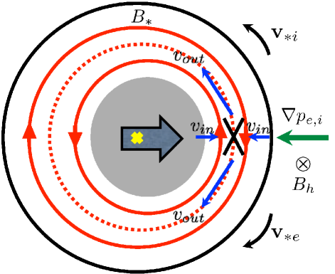
Figure 1: (Color) Sketch of the $m=1,n=1$ reconnection plane. Reconnecting (auxiliary) magnetic fields $B_{*}$ are in red with the rational surface $r_{s}$ indicated by the dotted red line. Plasma inflows $v_{in}$ and outflows $v_{out}$ are in blue with the reconnection site at the black X. The grey core moves from its initial position centered at the yellow X. The pressure gradient is the green arrow. The helical guide field $B_{h}$ and the diamagnetic drift velocities ${\bf v}_{*i}$ and ${\bf v}_{*e}$ are shown.

We propose that the increase in $v_{*i}$ and $v_{*e}$ as the pressure gradient self-consistently increases due to reconnection causes the left-hand side of Eq. (1) to increase. If Eq. (1) is never satisfied, reconnection is complete. If the pressure gradient becomes large enough, reconnection ceases. Since Eq. (1) can be satisfied even when free magnetic energy remains, this provides a possible mechanism for incomplete reconnection. This model departs from previous ones Biskamp (1981); Biskamp and Sato (1997); Park et al. (1987) as it concerns pressure gradients at the reconnection site rather than the magnetic islands.

This model complements, and may explain key global features of, recent observations at MAST Chapman et al. (2010). They observe that $|\nabla T_{e}|$ increases during a sawtooth period, peaking at the end of the crash (their Fig. 3), qualitatively consistent with the model. They also show that secondary ideal-MHD instabilities are destabilized at the end of the crash cycle. Reconnection would also play an important role in this process. When reconnection ceases, the electron-scale current sheet broadens, reducing the magnetic shear in a region where $|\nabla p|$ is large. Decreased shear is known to destabilize interchange instabilities (e.g. Freidberg (1987)).

To test the model, proof-of-principle numerical simulations are performed using F3D Shay et al. (2004), a two-fluid code employing a two-dimensional slab geometry with periodic boundary conditions. This geometry is appropriate because motion in the plane normal to the guide magnetic field is well described in two dimensions, toroidal effects are not expected to play a role on the short time scales in question (tens of $\mu{\rm s}$), and three-dimensional toroidal simulations employ unphysical forcing terms to obtain sawteeth Breslau et al. (2008). These simulations do not contain toroidal effects which lead to secondary ideal-MHD instabilities Chapman et al. (2010) because this facet of the evolution is outside the scope of this study. Electron pressure is evolved assuming an adiabatic ideal gas with a ratio of electron specific heats $\gamma_{e}=5/3$. Since the relative diamagnetic speed is the key parameter, ions are assumed cold for simplicity. Magnetic fields and mass densities are normalized to arbitrary values $B_{0}$ and $\rho_{0}$, velocities to the Alfvén speed $c_{A0}=B_{0}/(4\pi\rho_{0})^{1/2}$, lengths to the ion inertial length $d_{i0}=c/\omega_{pi}=(m_{i}^{2}c^{2}/4\pi\rho_{0}Z_{{\rm eff}}^{2}e^{2})^{1/2}$, times to the ion cyclotron time $\Omega_{ci0}^{-1}=(Z_{{\rm eff}}eB_{0}/m_{i}c)^{-1}$, electric fields to $E_{0}=c_{A0}B_{0}/c$, and pressures to $p_{0}=B_{0}^{2}/4\pi$, where $m_{i}$ is the ion mass, $c$ is the speed of light, $e$ is the proton charge, and $Z_{{\rm eff}}$ is the effective atomic number.

The coordinate system has $x$ parallel to the inflow (radial), $y$ parallel to the outflow (poloidal), and $z$ in the out-of-plane (toroidal) direction, invariant in the present two-dimensional simulations. The equilibrium has an in-plane magnetic field profile of a double Harris sheet,

$$B_{y}(x)=\tanh\left(\frac{x-L_{x}/4}{w_{0}}\right)-\tanh\left(\frac{x+L_{x}/4}{w_{0}}\right)+1,$$

where $L_{x}\times L_{y}=102.4\times 204.8$ is the system size and $w_{0}=0.5$ is the initial thickness of the current sheet. For this equilibrium, the toroidal mode number $n=0$ manifestly, so the rational surfaces are $x_{s}=\pm L_{x}/4=\pm 25.6$. We focus on a single mode because there is typically a dominant mode in sawteeth; the $n=0$ mode is chosen for simplicity, but is not expected to alter the conclusions. The mass density is initially $\rho=1$. The initial electron pressure profile is

$$p_{e}(x)\!\!\!\! =\frac{1}{2}\left(p_{1}+p_{2}\right)+\frac{1}{2}\left(p_{1}-p_{2}\right)\times$$

$$\left[\tanh\left(\frac{x+3L_{x}/8}{w_{p}}\right)-\tanh\left(\frac{x-3L_{x}/8}{w_{p}}\right)-1\right].$$

The pressure gradient is localized near $x=\pm 3L_{x}/8=\pm 38.4$ rather than at the rational surfaces $x_{s}$. Thus, $p_{e}$ at the reconnection site is initially uniform. The length scale of the pressure gradient is $w_{p}$ = 2. The guide magnetic field $B_{z}(x)$ has a mean value of $5$ with a profile that ensures initial pressure balance, $p+B^{2}/2={\rm constant}$.

The data we present are from simulations with a grid scale of $\Delta=0.05$. A test simulation with $\Delta=0.025$ confirms the resolution is sufficient. The equations employ fourth-order diffusion with coefficient $D_{4}=2\times 10^{-5}$ to damp noise at the grid scale; $D_{4}$ has been varied to ensure the key physics is not sensitive to it. The electron to ion mass ratio is 1/25. Simulations include no resistivity because experimental crash times are faster than collisional reconnection times. The presented simulations do not employ a parallel thermal conductivity, but test simulations with $\chi_{||}=0.08$ reveal no significant changes. Tearing is initiated by a small coherent perturbation to the in-plane magnetic field of amplitude $0.01$. It is known that secondary islands can spontaneously arise in reconnection simulations; due to symmetry, such islands would stay at the original X-line Loureiro et al. (2005). To prevent this, initial random magnetic perturbations of magnitude $2.0\times 10^{-5}$ break symmetry so secondary islands are ejected.

The principal simulation employs $p_{1}=5,p_{2}=25$ so $v_{*e}$ will exceed $v_{out}$ when the high pressure plasma convects in. Other simulation parameters are carefully chosen: $B_{z}\gg B_{y}$ as is relevant to sawteeth and $p_{e}$ is large enough so the ion Larmor radius $\rho_{s}=c_{s}/\Omega_{ci}$ exceeds the electron skin depth $d_{e}=c/\omega_{pe}$, allowing fast reconnection to proceed Aydemir (1992); Rogers et al. (2001). Here, $c_{s}=(\gamma_{e}Z_{{\rm eff}}T_{e}/m_{i})^{1/2}$ is the ion acoustic speed, and $T_{e}$ is the electron temperature.

Upon evolving the system, Hall reconnection occurs initially and the high pressure plasma convects towards the reconnection site as expected. The reconnection rate $E$, measured as the time rate of change of magnetic flux between the X-line and O-line, is plotted as the solid (red) line in Fig. 2(a). It increases from zero to its expected value near 0.1 Shay et al. (1999) by $t\sim 90$, where it reaches a steady-state with a single X-line. (The variation between $t=40$ and 90 is due to transient secondary island formation and coalescence.) At $t\simeq 195$, $E$ begins decreasing. It decreases to below zero, where it fluctuates for a number of Alfvén crossing times. Thus, reconnection has shut off.

To determine the cause, the electron diamagnetic speed $v_{*e}$ at the reconnection site is plotted as a function of time in Fig. 2(b) as the dashed (black) line. For comparison, the outflow speed $v_{out}$ is plotted as the solid (red) line. Asymmetric outflows occur when there is a pressure gradient in the outflow direction Murphy et al. (2010), and since such gradients self-consistently generate here, $v_{out}$ is calculated as the average of the maximum electron outflow speeds from either side of the reconnection site, averaged over $5d_{e}$ when turbulent.

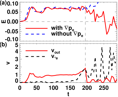
Figure 2: (Color online) (a) Reconnection rate $E$ as a function of time $t$ with and without a pressure gradient. (b) Diamagnetic drift speed $v_{*e}$ at the reconnection site and outflow speed $v_{out}$ vs. $t$.

Figure 2(b) reveals that $v_{*e}$ is small initially, but increases in time once the pressure gradient reaches the reconnection site at $t\simeq 140$. It increases until it becomes comparable to $v_{out}$ at $t\simeq 195$ (the vertical dashed line), the same time $E$ begins to decrease. Therefore, reconnection is throttled when Eq. (1) is first satisfied.

To ensure diamagnetic effects occur, the out-of-plane current density $J_{z}$ near the X-line is plotted in Fig. 3 (a) before ($t=125$) and (b) after ($t=180$) the pressure gradient arrives, with in-plane magnetic field lines superimposed. The guide field is in the $-z$-direction and $\nabla p_{e}$ is in the $-x$-direction. The reconnection site drifts in the $-y$-direction, the direction of ${\bf v}_{*e}$. Note, a secondary instability (recently speculated to be a drift instability Drake (2011)) appears. The increased variability of $v_{*e}$ and $E$ after $t\simeq 205$ are attributed to this instability.

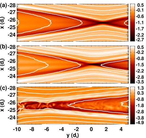
Figure 3: (Color) Out-of-plane current density $J_{z}$ zoomed in near the X-line with magnetic field lines superimposed (a) before ($t=125$), (b) after ($t=180$), and (c) significantly after ($t=210$) the pressure gradient reaches the reconnection site. The $x$ and $y$ axes correspond to the radial and poloidal directions, respectively.

To ensure the observed effect is caused by the pressure gradient, simulations with other pressure profiles are performed. When there is no gradient with $p_{1}=p_{2}=5$, there is no decrease in $E$, plotted as the dashed (blue) line in Fig. 2(a). The same is true for $p_{1}=p_{2}=25$ (not plotted). When $p_{1}=5,p_{2}=7$, no drop in reconnection rate is observed because the maximum $v_{*e}$ only reaches $\sim 1$, but $v_{out}\sim 2$ so Eq. (1) is never satisfied. In summary, the simulations confirm the basic prediction of the model: reconnection ceases when large enough pressure gradients self-consistently convect into the reconnection site despite the presence of free magnetic energy.

Post-cessation features are important for the subsequent dynamics. Figure 3(c) shows $J_{z}$ significantly after the pressure gradient reaches the reconnection site ($t=210$). The current layer clearly broadens as reconnection stops, reducing the magnetic shear at the reconnection site, as evidenced by the negative reconnection rate in Fig. 2(a). The reduced shear would make the system more prone to interchange instabilities, which were argued to occur in Ref. Chapman et al. (2010).

Equation (1) provides a quantitative prediction of the conditions at the end of sawteeth; we assess it with data from MAST Chapman et al. (2010). To transform into the plane of reconnection perpendicular to the $m=1,n=1$ helical direction, the reconnecting (auxiliary) field $B_{*}$ is related to the toroidal $B_{\varphi}$ and poloidal $B_{\theta}$ fields by

$$B_{*}(r)=B_{\theta}-\left(\frac{r}{R_{0}}\right)B_{\varphi}.$$ (2)

At MAST, $R_{0}=0.85\ {\rm m}$ Appel et al. (2008) while $B_{\varphi}\simeq 0.4\ {\rm T}$ and $B_{\theta}\simeq 0.15\ {\rm T}$ Chapman (2011). The rational surface $r_{s}$ is where $B_{*}=0$ in Eq. (2), which gives $r_{s}\simeq 0.32\ {\rm m}$. This result agrees well with Fig. 1(a) of Ref. Chapman et al. (2010). The helical guide field at $r_{s}$ is $B_{h}=B_{\varphi}(1+r_{s}/R_{0})\simeq 0.55\ {\rm T}$.

To test the model, Eq. (1) must be evaluated at the end of the sawtooth crash. The outflow speed scales with $c_{Ae}$, the electron Alfvén speed based on the field $B_{*e}$ upstream of the electron current layer. Assuming the large guide field limit with $B_{h}\gg B_{*}$ in the vicinity of $r_{s}$, the thickness of the electron current layer scales as the electron Larmor radius $\rho_{e}=v_{th,e}/\Omega_{ce}$ Horiuchi and Sato (1997), where $v_{th,e}=(\gamma_{e}T_{e}/m_{e})^{1/2}$ is the electron thermal speed and $\Omega_{ce}=eB/m_{e}c$ is the electron cyclotron frequency. Using $T_{e}\simeq 500\ {\rm eV}$ at $r_{s}$ Chapman et al. (2010) and $\gamma_{e}=5/3$, we find $\rho_{e}\simeq 0.013\ {\rm cm}$. To find $B_{*e}$, we evaluate Eq. (2) at $r_{s}\pm 2\rho_{e}$ Jemella et al. (2003), which gives $B_{*e}\simeq 5.9\times 10^{-5}\ {\rm T}$, justifying the strong guide field assumption. Using this value gives $v_{out}\approx 14.2\ {\rm km/s}$, where $n_{e}\simeq 6\times 10^{19}\ {\rm m^{-3}}$ is estimated from Fig. 2 in Ref. Chapman et al. (2010).

To estimate $v_{*e}$, note $|\nabla p_{e}|/n_{e}=|\nabla T_{e}|+T_{e}(|\nabla n_{e}|/n_{e})$. The right-hand side is estimated at the end of the crash from Figs. 1(e), 2 and 3 of Ref. Chapman et al. (2010) to be $|\nabla p_{e}|/n_{e}\simeq 7400\ {\rm eV/m}$. Then, the electron diamagnetic speed is $v_{*e}=|\nabla p_{e}|/(qn_{e}B_{h})\approx 13.5\ {\rm km/s}$. Equation (1) includes ion diamagnetic effects, but complementary ion data is unavailable Chapman (2011). Assuming the ion temperature has a similar profile as the electrons with $T_{e}>T_{i}$, we expect $v_{*e}<|v_{*i}|+|v_{*e}|<2v_{*e}$. Thus, the two speeds agree rather well, showing the agreement with the data is also quantitative.

As a further consistency check, we compare the speed of the core to the inflow speed. The the core’s speed is estimated from Figs. 1(d-f) of Ref. Chapman et al. (2010) by dividing its displacement ($\simeq 0.08\ {\rm m}$) by the elapsed time ($\simeq 0.04\ {\rm ms}$), giving a speed of $\sim 2\ {\rm km/s}$. The reconnection inflow speed scales like $0.1c_{Ai}$ Shay et al. (2004), where $c_{Ai}$ is the ion Alfvén speed based on the field $B_{*i}$ upstream of the ion current layer. The ion layer thickness with a large guide field scales like the ion Larmor radius $\rho_{s}$ Zakharov et al. (1993). Using $Z_{{\rm eff}}\sim 1$ Tournianski et al. (2005) and $m_{i}=2m_{p}$ for a deuterium plasma Appel et al. (2008), we find $\rho_{s}∼\sim 0.77\ {\rm cm}$. As in the calculation of $B_{*e}$, we evaluate Eq. (2) at $r_{s}\pm 2\rho_{s}$, giving $B_{*i}=6.7\times 10^{-3}\ {\rm T}$. Then, $c_{Ai}\approx 13\ {\rm km/s}$, so the inflow speed is $\simeq 1.3\ {\rm km/s}$. Thus, the inflow speed is comparable to the speed of the core, as predicted.

For tokamak applications, Eq. (1) may be recast in terms of more familiar quantities. Assuming $v_{out}\sim c_{Ae}$ in Eq. (1) and rewriting Eq. (2) in terms of $q$ and expanding to lowest order in $r$ for a small displacement ($2\rho_{e}$) from $r_{s}$, $B_{*e}\simeq B_{\theta}q^{\prime}2\rho_{e}$, where the prime denotes a radial derivative. Thus, Eq. (1) becomes

$$\frac{1}{eB_{h}}\left|\frac{p_{i}^{\prime}}{Z_{{\rm eff}}n_{i}}+\frac{p_{e}^{\prime}}{n_{e}}\right|>\frac{2\rho_{e}B_{\theta}}{\sqrt{4\pi m_{e}n_{e}}}q^{\prime},$$ (3)

where all quantities are evaluated at $r_{s}$. This expression is reminiscent of the condition on $p^{\prime}$ and $q^{\prime}$ for suppression of sawteeth derived from linear tearing theory Zakharov et al. (1993); Levinton et al. (1994).

In conclusion, we have described a model for incomplete reconnection in sawtooth crashes, tested the basic physics with numerical simulations, and shown it is consistent with data from MAST. Interestingly, recent simulations of sawteeth revealed complete reconnection in MHD, but incomplete reconnection in extended-MHD with electron and ion diamagnetic effects Breslau et al. (2007, 2008); the present result may be relevant. Equation (1) may be useful for low-dimensional transport modeling, which currently use ad hoc models to achieve incomplete reconnection Bateman et al. (2006). The present results are machine independent, so they should apply both to existing tokamaks and future ones such as ITER.

In future studies, the model should be tested with other extended-MHD effects such as ion diamagnetic effects and higher $\chi_{||}$. The restriction on toroidal mode number $n$ should be relaxed. The effect of the electron pressure profile on the dynamics and the secondary (drift) instability should be addressed; this may need to utilize particle-in-cell simulations. Including 3D toroidal geometry is critical for exploring secondary ideal-MHD instabilities. Comparisons to multiple tokamak discharges should be done to test the scaling.

We thank I. T. Chapman for providing MAST data and thank J. F. Drake, D. C. Pace, M. A. Shay, and M. Swisdak for helpful conversations. The authors gratefully acknowledge support by NSF grant PHY-0902479. This research used resources at National Energy Research Scientific Computing Center.

References

- (1)
- von Goeler et al. (1974) S. von Goeler, W. Stodiek, and N. R. Sautoff, Phys. Rev. Lett. 33, 1201 (1974).
- Hender et al. (2007) T. C. Hender, J. C. Wesley, J. Bialek, A. Bondeson, A. H. Boozer, R. J. Buttery, A. Garofalo, T. P. Goodman, R. S. Granetz, Y. Gribov, et al., Nucl. Fusion 47, S128 (2007).
- Kadomtsev (1975) B. B. Kadomtsev, Sov. J. Plasma Phys. 1, 389 (1975).
- Edwards et al. (1986) A. W. Edwards, D. J. Campbell, W. W. Engelhardt, H. U. Farhbach, R. D. Gill, R. S. Granetz, S. Tsuji, B. J. D. Tubbing, A. Weller, J. Wesson, et al., Phys. Rev. Lett. 57, 210 (1986).
- Yamada et al. (1994) M. Yamada, F. M. Levinton, N. Pomphrey, R. Budny, J. Manickam, and Y. Nagayama, Phys. Plasmas 1, 3269 (1994).
- Soltwisch (1992) H. Soltwisch, Plasma Phys. Control. Fusion 34, 1669 (1992).
- Lichtenberg et al. (1992) A. J. Lichtenberg, K. Itoh, S. I. Itoh, and A. Fukuyama, Nucl. Fusion 32, 495 (1992).
- Biskamp (1981) D. Biskamp, Phys. Rev. Lett. 46, 1522 (1981).
- Biskamp and Sato (1997) D. Biskamp and T. Sato, Phys. Plasmas 4, 1326 (1997).
- Park et al. (1987) W. Park, D. A. Monticello, and T. K. Chu, Phys. Fluids 30, 285 (1987).
- Wang and Bhattacharjee (1995) X. Wang and A. Bhattacharjee, Phys. Plasmas 2, 171 (1995).
- Coppi et al. (1988) B. Coppi, R. J. Hastie, S. Migliuolo, F. Pegoraro, and F. Porcelli, Phys. Lett. A 132, 267 (1988).
- White et al. (1989) R. B. White, M. N. Bussac, and F. Romanelli, Phys. Rev. Lett. 62, 539 (1989).
- Porcelli (1991) F. Porcelli, Plasma Phys. Control. Fusion 33, 1601 (1991).
- Holmes et al. (1989) J. A. Holmes, B. A. Carreras, and L. A. Charlton, Phys. Fluids B 1, 788 (1989).
- Kleva (1992) R. G. Kleva, Phys. Fluids B 4, 218 (1992).
- Kleva and Guzdar (2002) R. G. Kleva and P. N. Guzdar, Phys. Plasmas 9, 3013 (2002).
- Porcelli et al. (1996) F. Porcelli, D. Boucher, and M. N. Rosenbluth, Plasma Phys. Control. Fusion 38, 2163 (1996).
- Swisdak et al. (2003) M. Swisdak, J. F. Drake, M. A. Shay, and B. N. Rogers, J. Geophys. Res. 108, 1218 (2003).
- Chapman et al. (2010) I. T. Chapman, R. Scannell, W. A. Cooper, J. P. Graves, R. J. Hastie, G. Naylor, and A. Zocco, Phys. Rev. Lett. 105, 255002 (2010).
- Zakharov et al. (1993) L. Zakharov, B. Rogers, and S. Migliuolo, Phys. Fluids B 5, 2498 (1993).
- Rogers and Zakharov (1995) B. Rogers and L. Zakharov, Phys. of Plasmas 2, 3420 (1995).
- Germaschewski et al. (2006) K. Germaschewski, A. Bhattacharjee, C. S. Ng, X. Wang, and L. Chacon, in Bull. Am. Phys. Soc. (2006), vol. 51, p. 312.
- Bhattacharjee et al. (2008) A. Bhattacharjee, K. Germaschewski, L. Nei, and H. Yang, in Eos Trans. AGU (AGU, San Francisco, 2008), vol. 89(53) of Fall Meet. Suppl., pp. Abstract SM21B–04.
- Freidberg (1987) J. P. Freidberg, Ideal Magnetohydrodynamics (Springer, 1987).
- Shay et al. (2004) M. A. Shay, J. F. Drake, M. Swisdak, and B. N. Rogers, Phys. Plasmas 11, 2199 (2004).
- Breslau et al. (2008) J. A. Breslau, C. R. Sovinec, and S. C. Jardin, Commun. Comput. Phys. 4, 647 (2008).
- Loureiro et al. (2005) N. F. Loureiro, S. C. Cowley, W. D. Dorland, M. G. Haines, and A. A. Schekochihin, Phys. Rev. Lett. 95, 235003 (2005).
- Aydemir (1992) A. Y. Aydemir, Phys. Fluids B 4, 3469 (1992).
- Rogers et al. (2001) B. N. Rogers, R. E. Denton, J. F. Drake, and M. A. Shay, Phys. Rev. Lett. 87, 195004 (2001).
- Shay et al. (1999) M. A. Shay, J. F. Drake, B. N. Rogers, and R. E. Denton, Geophys. Res. Lett. 26, 2163 (1999).
- Murphy et al. (2010) N. A. Murphy, C. R. Sovinec, and P. A. Cassak, J. Geophys. Res. 115, A09206 (2010).
- Drake (2011) J. F. Drake (2011), Private Communication.
- Appel et al. (2008) L. C. Appel, T. Fülöp, M. J. Hole, H. M. Smith, S. D. Pinches, R. G. L. Vann, and the MAST team, Plasma Phys. Control. Fusion 50, 115011 (2008).
- Chapman (2011) I. T. Chapman (2011), Private Communication.
- Horiuchi and Sato (1997) R. Horiuchi and T. Sato, Phys. Plasmas 4, 277 (1997).
- Jemella et al. (2003) B. D. Jemella, M. A. Shay, J. F. Drake, and B. N. Rogers, Phys. Rev. Lett. 91, 125002 (2003).
- Tournianski et al. (2005) M. R. Tournianski, R. J. Akers, P. G. Carolan, and D. L. Keeling, Plasma Phys. Control. Fusion 47, 671 (2005).
- Levinton et al. (1994) F. M. Levinton, L. Zakharov, S. H. Batha, J. Manickam, and M. C. Zarnstorff, Phys. Rev. Lett. 72, 2895 (1994).
- Breslau et al. (2007) J. A. Breslau, S. C. Jardin, and W. Park, Phys. Plasmas 14, 056105 (2007).
- Bateman et al. (2006) G. Bateman, C. N. Nguyen, A. H. Kritz, and F. Porcelli, Phys. Plasmas 13, 072505 (2006).