Extended supersymmetry of the self-isospectral crystalline and soliton chains

Abstract

We study supersymmetric structure of the self-isospectral crystalline chains formed by $N$ copies of the mutually displaced one-gap Lamé systems. It is generated by the $N(N-1)$ integrals of motion which are the first order matrix differential operators, by the same number of the nontrivial second order integrals, and by the $N$ third order Lax integrals. We show that the structure admits distinct alternatives for a grading operator, and in dependence on its choice one of the third order matrix integrals plays either the role of the bosonic central charge or the role of the fermionic supercharge to be a square root of the spectral polynomial. Yet another peculiarity is that the set of all the second order integrals of motion generates a nonlinear sub-superalgebra. We also investigate the associated self-isospectral soliton chains, and discuss possible physical applications of the unusual extended supersymmetry.

1 Introduction

Quantum periodic finite-gap systems are associated with completely integrable models. Any such a system is characterized by a proper nontrivial integral of motion that is a higher order Lax operator $\mathcal{P}$ [1]. In the infinite period limit they transform into reflectionless (soliton) systems. Their band structure is effectively encrypted in a Burchnall-Chaundy operator identity [2, 3] that can be presented in a form of a supersymmetric-like relation [4]

$$\{\mathcal{P},\mathcal{P}\}=2P(H),$$ (1.1)

where $P(H)$ is a spectral polynomial and $H$ is a Hamiltonian.

Because of the presence of the nontrivial integral $\mathcal{P}$, a supersymmetric extension of finite-gap systems has a more rich structure in comparison with that of a usual $N=2$ supersymmetric quantum mechanics. An example of a physical system with such an unusual supersymmetry is provided by a model of a non-relativistic electron in periodic magnetic and electric fields [21]. In a generic case of the $N=2$ superextension of an $n$-gap system by means of a Crum-Darboux transformation of the order $m$, $1\leq m<2n+1$, where $2n+1$ is a number of band edge states, supersymmetric finite-gap system is characterized by two further supercharges of the order $(2n+1-m)$ [21]. The anti-commutator of supercharges of the orders $m$ and $(2n+1-m)$ generates the Lax integral of the order $2n+1$. Another important peculiarity is that such superextended systems admit various choices for the grading operator. For some of them, matrix diagonal Lax integral takes a role of one of the supercharges that annihilates all the $2(2n+1)$ band edge states of the extended system. Unlike the anti-diagonal supercharges of the orders $m$ and $(2n+1-m$), it also distinguishes the left- and right- moving Bloch modes inside the allowed bands [22]. This is similar to a role played by a momentum operator for a free particle that can be treated as a zero-gap system.

Sometimes, a supersymmetric partner happens to be just a spatially displaced initial finite-gap periodic or non-periodic system. The Witten index takes then a zero value for such a self-isospectral system [17] even in the case of unbroken supersymmetry [14, 15, 23].

Recently, it was observed [22] that a phase transition between the kink-antikink and kink crystalline phases in the Gross-Neveu model [24, 25, 26, 27, 28] is accompanied by the structural changes in the associated supersymmetric self-isospectral one-gap periodic Lamé system. Any of the two first order supercharges of the latter can be taken as the Bogoliubov-de Gennes Hamiltonian in the Andreev approximation, in which superpotential is identified with a gap function (a condensate field). The first order supercharges are constructed from the Darboux displacement generators of the associated second order Schrödinger system. Yet another peculiarity of such a system is that the first order Bogoliubov-de Gennes Hamiltonian possesses its own, exotic hidden nonlinear supersymmetry [22]. A certain infinite period limit applied to the one-gap self-isospectral system reproduces either the supersymmetric structure of the Dashen, Hasslacher, and Neveu kink-antikink baryons [29] as a Darboux dressed form of a free massive Dirac particle [30], or superextended version of the Callan-Coleman-Gross-Zee kink solution [29, 31] of the Gross-Neveu model [22].

A pair of the second order supercharges of the $N=2$ superextended one-gap Lamé system is generated by a sequence of the two first order Darboux displacements, while the Lax operators of the mutually shifted Lamé subsystems are produced by closed third order Crum-Darboux loops. The second order supercharges and the third order Lax integrals include a dependence on an auxiliary, virtual displacement parameter. It is natural to try to extend the model by taking $N>2$ mutually displaced copies of Lamé systems. This produces then the question:

• What supersymmetric structure will be generated in such an extended Lamé system by considering the higher order unclosed ($m>2$) and closed ($m>3$) sequences of Darboux displacements?

In the present paper we study the supersymmetric structure of the self-isospectral crystalline chain of mutually displaced one-gap Lamé systems, and investigate in the same context the associated self-isospectral non-periodic (soliton) chains of reflectionless Pöschl-Teller systems.

The paper is organized as follows. In the next section we construct the first order Darboux displacement generators for the one-gap Lamé system. In section 3 we apply them to construct self-isospectral chains of Lamé systems, and investigate the higher order generalizations of the Darboux displacement generators. In section 4 we study a general structure of the exotic nonlinear supersymmetry of the self-isospectral crystalline $N$-term chain. Section 5 is devoted to the discussion of alternative choices for the $\mathbb{Z}_{2}$-grading operator admitted by such an extended supersymmetric structure. In section 6 general theory is illustrated by an example of the $N=3$ crystalline chain. In section 7 we consider the infinite period limit that produces a self-isospectral non-periodic chain and its supersymmetric structure. In the last section we conclude with a discussion of possible physical applications of the revealed unusual nonlinear supersymmetry.

2 Darboux displacement generators: periodic case

Consider a one-dimensional self-adjoint Schrödinger Hamiltonian $H(x)=-\frac{d^{2}}{dx^{2}}+V(x)$ with a periodic potential $V(x)$. Require that the system admits a family of the first order Darboux displacement generators $\mathcal{D}(x;\lambda)=\frac{d}{dx}+\varphi(x;\lambda)$,

$$\mathcal{D}(x;\lambda)H(x)=H(x+\lambda)\mathcal{D}(x;\lambda),$$ (2.1)

which depends on a continuous parameter $\lambda$. Then it can be shown that $V(x)$ has to be a one-gap Lamé potential [15, 19]. The Jacobi form of the one-gap Lamé system is [32]

$$H(x)=-\frac{d^{2}}{dx^{2}}+2k^{2}\mathrm{sn}^{2}\,x-k^{2}\,.$$ (2.2)

A modular parameter $k$, $0<k<1$, fixes a real, $2{\rm\bf K}$, and imaginary, $2{\mathbf{i}}{\rm\bf K}^{\prime}$, periods of the potential. Here and in what follows we do not indicate explicitly the dependence of elliptic and related functions on $k$, and use a notation ${\mathbf{i}}=\sqrt{-1}$ for imaginary unit. The chosen value of the additive constant fixes the level of the lower edge of the valence band to be zero, and the one-gap spectrum of (2.2) is $\sigma(H)=[0,k^{\prime 2}]\cup[1,\infty)$, where $0<k^{\prime}<1$ is a complementary modular parameter, $k^{\prime 2}=1-k^{2}$. The infinite period limit ($k\rightarrow 1$ $\Rightarrow$ $2{\rm\bf K}\rightarrow\infty$, $2{\mathbf{i}}{\rm\bf K}^{\prime}\rightarrow{\mathbf{i}}\pi$, $\mathrm{sn}\,x\rightarrow\tanh x$) of (2.2) corresponds to a reflectionless Pöschl-Teller system with one bound state in the spectrum, while in another limit $k\rightarrow 0$, (2.2) reduces to a free particle system.

To construct a one-parametric Darboux displacement generator, we discuss shortly some properties of Lamé system (2.2). Solutions of the stationary equation $H\Psi(x)=E\Psi(x)$ are given by the Bloch functions of the form

$$\Psi_{\pm}^{\alpha}(x)=\frac{{\rm H}(x\pm\alpha)}{\Theta(x)}\exp\left[\mp x{\rm Z}(\alpha)\right]\,,\qquad E=\mathrm{dn}^{2}\alpha,$$ (2.3)

where ${\rm H}$, $\Theta$ and ${\rm Z}$ are the Eta, Theta and Zeta Jacobi functions [32, 33]. Under translation for the period, they transform as

$$\Psi_{\pm}^{\alpha}(x+2{\rm\bf K})=\exp[\mp{\mathbf{i}}2{\rm\bf K}\kappa(\alpha)]\Psi_{\pm}^{\alpha}(x)\,,\quad\kappa(\alpha)=\frac{\pi}{2{\rm\bf K}}-{\mathbf{i}}{\rm Z}(\alpha)\,,$$ (2.4)

where $\kappa(\alpha)$ is a quasi-momentum. Energy $E$ is given here as a function $E(\alpha)=\mathrm{dn}^{2}\alpha$ of a complex parameter $\alpha$. This is an elliptic function with the same modular parameter $k$, and its period parallelogram in complex plane $\alpha\in\mathbb{C}$ is a rectangle with vertices in $0$, $2{\rm\bf K}$, $2{\rm\bf K}+2{\mathbf{i}}{\rm\bf K}^{\prime}$, and $2{\mathbf{i}}{\rm\bf K}^{\prime}$. On the border of the indicated period parallelogram, function $\mathrm{dn}\,\alpha$ takes real or pure imaginary values, and so, $E$ is real. The vertical sides $\alpha={\mathbf{i}}\beta+{\rm\bf K}$, $0\leq\beta\leq{\rm\bf K}^{\prime}$, and $\alpha={\mathbf{i}}\beta$, $0\leq\beta<{\rm\bf K}^{\prime}$, correspond, respectively, to the valence, $0\leq E\leq k^{\prime 2}$, and the conduction, $1\leq E<\infty$, bands, where the quasi-momentum $\kappa(\alpha)$ is real. The horizontal sides $\alpha={\mathbf{i}}{\rm\bf K}^{\prime}+\beta$ and $\alpha=\beta$ with $0<\beta<{\rm\bf K}$ correspond to the prohibited bands $-\infty<E<0$ and $k^{\prime 2}<E<1$, where $\kappa(\alpha)$ takes complex values. Inside the allowed bands, (2.3) are the two Bloch modes propagating to the left (the upper index) and to the right (the lower index). On the edges of the bands, they reduce to the standing waves described by the periodic, $\mathrm{dn}\,x=\mathrm{dn}\,(x+2{\rm\bf K})$ ($E=0$), and antiperiodic, $\mathrm{cn}\,x=-\mathrm{cn}\,(x+2{\rm\bf K})$ ($E=k^{\prime 2}$) and $\mathrm{sn}\,x=-\mathrm{sn}(x+2{\rm\bf K})$ ($E=1$), functions.

Like the ground state $\mathrm{dn}\,x$ ($\alpha={\rm\bf K}+{\mathbf{i}}{\rm\bf K}^{\prime}$, $E=0$), non-physical Hamiltonian eigenstates in the lower prohibited band $-\infty<E<0$ are nodeless functions, which can be used to construct a one-parametric family of the first order Darboux generators. As $\mathrm{dn}\,(-u)=\mathrm{dn}\,(u+2{\rm\bf K})=-\mathrm{dn}\,(u+2{\mathbf{i}}{\rm\bf K}^{\prime})=\mathrm{dn}\,u$, it is convenient to introduce a notation $\alpha=-2\tau+{\mathbf{i}}{\rm\bf K}^{\prime}$, and assume that $\tau\in\mathbb{R}$ while keeping in mind that $E\rightarrow-\infty$ for $\tau\rightarrow n{\rm\bf K}$, $n\in\mathbb{Z}$. By shifting the argument, $x\rightarrow x+\tau$, for the wave function (2.3) with the upper index we get $\Psi^{-2\tau+{\mathbf{i}}{\rm\bf K}^{\prime}}_{+}(x+\tau)=c(\tau)F(x;\tau)$, where $c(\tau)$ is a nonzero $x$-independent multiplier, and

$$\frac{\Theta(x-\tau)}{\Theta(x+\tau)}\exp[x\mathfrak{z}(\tau)]\equiv F(x;\tau)\,.$$ (2.5)

Here

$$\mathfrak{z}(\tau)={\rm Z}(2\tau+{\mathbf{i}}{\rm\bf K}^{\prime})+{\mathbf{i}}\frac{\pi}{2{\rm\bf K}}={\rm Z}(2\tau)+\frac{\mathrm{cn}\,2\tau\mathrm{dn}\,2\tau}{\mathrm{sn}\,2\tau\,}$$ (2.6)

is, up to a factor $-{\mathbf{i}}$, a quasi-momentum of the Bloch state (2.5), $\mathfrak{z}(\tau)=-{\mathbf{i}}\kappa(-2\tau+{\mathbf{i}}{\rm\bf K}^{\prime})$, that is an odd function of $\tau$. A nodeless function $F(x;\tau)$ is quasi-periodic in $x$, $F(x+2{\rm\bf K};\tau)=\exp[2{\rm\bf K}\mathfrak{z}(\tau)]F(x;\tau)$, periodic in $\tau$, $F(x;\tau+2{\rm\bf K})=F(x;\tau)$, and for $x\neq 0$ it undergoes infinite jumps from $0$ to $+\infty$ at $\tau=n{\rm\bf K}$, $n\in\mathbb{Z}$. It also satisfies the relations $F(x;-\tau)=F(-x;\tau)={1}/{F(x;\tau)}$. In the case of the ground state $\mathfrak{z}(-{\rm\bf K}/2)=0$, and function (2.5) reduces to a periodic function $(k^{\prime})^{-1/2}\mathrm{dn}(x-\frac{{\rm\bf K}}{2})$.

Let us consider now a first order differential operator

$$\mathcal{D}(x;\tau)=F(x;\tau)\frac{d}{dx}\frac{1}{F(x;\tau)}=\frac{d}{dx}-\Delta(x;\tau),\qquad\mathcal{D}^{\dagger}(x;\tau)=-\mathcal{D}(x;-\tau)\,,$$ (2.7)

whose zero mode is $F(x;\tau)$, $\mathcal{D}(x;\tau)F(x;\tau)=0$. Function $\Delta(x;\tau)={F\,{}^{\prime}(x;\tau)}/{F(x;\tau)}$, $F\,{}^{\prime}(x;\tau)=\frac{\partial}{\partial x}F(x;\tau)$, reads

$$\Delta(x;\tau) = \mathfrak{z}(\tau)+{\rm Z}(x-\tau)-{\rm Z}(x+\tau)$$ (2.8)

$$= \frac{\mathrm{cn}\,2\tau\mathrm{dn}\,2\tau}{\mathrm{sn}\,2\tau}+k^{2}\mathrm{sn}\,2\tau\mathrm{sn}(x-\tau)\mathrm{sn}(x+\tau)\,.$$

It obeys the Riccati equations

$$\Delta^{2}(x;\tau)\pm\Delta^{\prime}(x;\tau)=2k^{2}\mathrm{sn}^{2}(x\pm\tau)-k^{2}+\varepsilon(\tau)\,,$$ (2.9)

where

$$\varepsilon(\tau)=-E(-2\tau+{\mathbf{i}}{\rm\bf K}^{\prime})=\mathrm{cn}^{2}2\tau/\mathrm{sn}^{2}2\tau\,.$$ (2.10)

Another important property is that the following three-term linear combination,

$$\Delta(x;\tau)+\Delta(x+\tau+\lambda;\lambda)+\Delta(x+\lambda;-\tau-\lambda)$$

$$=\mathfrak{z}(\tau)+\mathfrak{z}(\lambda)+\mathfrak{z}(-\tau-\lambda)\equiv g(\tau,\lambda)\,,$$ (2.11)

is $x$-independent. The function $g(\tau,\lambda)$ possesses the symmetry properties $g(\tau,\lambda)=g(\lambda,\tau)=g(\tau,-\lambda-\tau)=-g(-\tau,-\lambda)$ and can be presented in a form

$$g(\tau,\lambda)=\frac{1-\mathrm{cn}\,2\tau\,\mathrm{cn}\,2\lambda\,\mathrm{cn}\,2(\tau+\lambda)}{\mathrm{sn}\,2\tau\,\mathrm{sn}\,2\lambda\,\mathrm{sn}\,2(\tau+\lambda)}\,.$$ (2.12)

From Eqs. (2.6) and (2.7) we find a relation $\Delta(\xi;\tau)=g\big{(}\frac{1}{2}(\xi-\tau-{\mathbf{i}}{\rm\bf K}^{\prime});\tau\big{)}$, i.e. by (2.11) $\Delta(\xi;\tau)$ can be presented by a three-term sum of quasi-momenta taken at three values of arguments which sum up to the zero. We also will need the identity

$$\Delta^{\prime}(x+\tau+\lambda;\lambda)-\Delta(x+\lambda;\tau+\lambda)\Delta(x+\tau+\lambda;\lambda)+g(\tau,\lambda)\Delta(x;\tau)=$$

$$-\frac{1}{2}(\Delta^{2}(x;\tau)+\Delta^{\prime}(x;\tau)+\delta(\tau))\,,\quad{\rm where}\quad\delta(\tau)=1+k^{2}-3\mathrm{sn}^{-2}2\tau\,,$$ (2.13)

which follows from (2.9) and (2.11).

By the Riccati equations (2.9), the operators (2.7) factorize the Lamé Hamiltonian (2.2),

$$\mathcal{D}^{\dagger}(x;\tau)\mathcal{D}(x;\tau)=H(x+\tau)+\varepsilon(\tau)\,,\qquad\mathcal{D}(x;\tau)\mathcal{D}^{\dagger}(x;\tau)=H(x-\tau)+\varepsilon(\tau)\,,$$ (2.14)

with (2.10) playing a role of a factorization constant.

Note here that the second eigenstate $\Psi^{-2\tau+{\mathbf{i}}{\rm\bf K}^{\prime}}_{-}(x+\tau)$ of the shifted Lamé Hamiltonian operator (2.2) reduces, up to an inessential $\tau$-dependent multiplier, to $F(x+2\tau;-\tau)$, that is coherent with a relation $E(-2\tau+{\mathbf{i}}{\rm\bf K}^{\prime})=E(2\tau+{\mathbf{i}}{\rm\bf K}^{\prime})$. In correspondence with this observation, a change $\tau\rightarrow-\tau$ in the first relation from (2.14) and a subsequent shift $x\rightarrow x+2\tau$ transform this first factorization into an equivalent form $\mathcal{D}(x+2\tau;\tau)\mathcal{D}^{\dagger}(x+2\tau;\tau)=H(x+\tau)+\varepsilon(\tau)$, that is just the second relation from (2.14) with the argument $x$ shifted for $2\tau$.

From (2.14) it follows that (2.7) are the sought for Darboux displacement generators,

$$\mathcal{D}(x;\tau)H(x+\tau)=H(x-\tau)\mathcal{D}(x;\tau)\,,\qquad\mathcal{D}^{\dagger}(x;\tau)H(x-\tau)=H(x+\tau)\mathcal{D}^{\dagger}(x;\tau).$$ (2.15)

As $\mathcal{D}^{\dagger}(x;\tau)=-\mathcal{D}(x;-\tau)$, it is sufficient to consider only the first intertwining relation from (2.15) while the second follows from it via a simple change $\tau\rightarrow-\tau$.

3 Chains of one-gap Lamé systems

In this section we construct higher order generalizations of Darboux generators, that will lead us naturally to the chains of Darboux-displaced one-gap Lamé systems.

A mutual spatial Darboux displacement between the two systems in (2.15) is $2\tau$ while their ‘average coordinate’ is $x$. For generalization it is convenient to characterize each of the two related systems by its own shift parameter by introducing the notations

$$\tau_{ab}=\frac{1}{2}(\tau_{b}-\tau_{a})=-\tau_{ba}\,,\qquad x_{ab}=x+\frac{1}{2}(\tau_{a}+\tau_{b})=x_{ba}.$$ (3.1)

Then $x_{ab}+\tau_{ab}=x+\tau_{b}$, $x_{ab}-\tau_{ab}=x+\tau_{a}$, and relations (2.14), (2.15) can be presented in the form

$$\mathcal{D}_{ab}\mathcal{D}^{\dagger}_{ab}=-\mathcal{D}_{ab}\mathcal{D}_{ba}=H_{a}+\varepsilon_{ab},$$ (3.2)

$$\mathcal{D}_{ab}H_{b}=H_{a}\mathcal{D}_{ab},$$ (3.3)

where we have introduced further notations

$$\mathcal{D}_{ab}=\mathcal{D}(x_{ab};\tau_{ab})=-\mathcal{D}^{\dagger}_{ba},\qquad H_{a}=H(x+\tau_{a}),\qquad\varepsilon_{ab}=\varepsilon(\tau_{ab})=\varepsilon_{ba}\,,$$ (3.4)

see Fig. 1. Since the superpotential $\Delta$, the Darboux displacement generator $\mathcal{D}_{ab}$ and the factorization constant $\varepsilon_{ab}$ blow up at $\tau_{ab}=n{\rm\bf K}$, $n\in\mathbb{Z}$, we suppose that $\tau_{ab}\neq n{\rm\bf K}$.

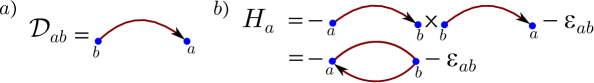
Figure 1: a) The Darboux displacement generator $\mathcal{D}_{ab}$ transforms eigenstates of $H_{b}$ into those of the translated system $H_{a}$, see (3.3). b) The Hamiltonian $H_{a}$ as a sequence of the two Darboux displacements (3.2).

Making use of the relation (3.3), one can define the second order operator

$$\mathcal{B}_{ab/\lambda}=\mathcal{D}_{a\lambda}\mathcal{D}^{\dagger}_{\lambda b}=-\mathcal{D}_{a\lambda}\mathcal{D}_{\lambda b}\,,\qquad\mathcal{B}^{\dagger}_{ab/\lambda}=\mathcal{B}_{ba/\lambda}\,,$$ (3.5)

where as for $\tau_{ab}$, we assume that $\tau_{a\lambda},\,\tau_{\lambda b}\neq n{\rm\bf K}$. Like the first order operator $\mathcal{D}_{ab}$, it intertwines the same two systems $H_{a}$ and $H_{b}$,

$$\mathcal{B}_{ab/\lambda}H_{b}=H_{a}\mathcal{B}_{ab/\lambda},$$ (3.6)

via a chain of the two Darboux displacements, $\mathcal{B}_{ab/\lambda}H_{b}=-\mathcal{D}_{a\lambda}\mathcal{D}_{\lambda b}H_{b}=-\mathcal{D}_{a\lambda}H_{\lambda}\mathcal{D}_{\lambda b}=-H_{a}\mathcal{D}_{a\lambda}\mathcal{D}_{\lambda b}=H_{a}\mathcal{B}_{ab/\lambda}$. In this chain, there appears an intermediate system $H_{\lambda}$, which from the viewpoint of our pair of basic systems $H_{a}$ and $H_{b}$ is of a virtual, auxiliary nature. To stress a virtual nature of the displacement parameter $\lambda$, we indicate it in a special way (with slash) in notation for the second order Crum-Darboux intertwining operator $\mathcal{B}$. From (3.5) we find a relation

$$\mathcal{B}_{aa/\lambda}=\mathcal{D}_{a\lambda}\mathcal{D}^{\dagger}_{a\lambda}=H_{a}+\varepsilon_{a\lambda}\,.$$ (3.7)

Hence, $\mathcal{B}_{ab/\lambda}$ is a kind of a non-Hermitian generalization of the Lamé Hamiltonian operator. In correspondence with (3.7), the second order intertwiner $\mathcal{B}_{ab/\lambda}$, unlike $\mathcal{D}_{ab}$, is well defined (for $\tau_{a\lambda},\,\tau_{\lambda b}\neq n{\rm\bf K}$) also in the case when $\tau_{ab}=n{\rm\bf K}$. The virtual parameter on the right-hand side in (3.7) appears only in the additive term. We also have

$$\mathcal{B}_{ab/\lambda}\mathcal{B}^{\dagger}_{ab/\lambda}=\mathcal{B}_{ab/\lambda}\mathcal{B}_{ba/\lambda}=(H_{a}+\varepsilon_{a\lambda})(H_{a}+\varepsilon_{b\lambda})\,.$$ (3.8)

Making use of (2.13), we find that a specific linear combination of the second, $\mathcal{B}$, and the first order, $\mathcal{D}$, intertwining operators,

$$\mathcal{Y}_{ab}=-\mathcal{B}_{ab/\lambda}-g_{ab\lambda}\mathcal{D}_{ab}\,,\qquad\mathcal{Y}^{\dagger}_{ab}=\mathcal{Y}_{ba}\,,$$ (3.9)

does not depend on the virtual parameter $\lambda$, where we have introduced a notation

$$g_{ab\lambda}\equiv g(\tau_{ab},\tau_{\lambda a})=\mathfrak{z}(\tau_{ab})+\mathfrak{z}(\tau_{b\lambda})+\mathfrak{z}(\tau_{\lambda a})\,$$ (3.10)

for a function of displacement parameters, which is completely antisymmetric in the indices, $g_{ab\lambda}=-g_{ba\lambda}=-g_{a\lambda b}$. Note the cyclic order of the indices on the r.h.s. of (3.10). The explicit form of the intertwining operator $\mathcal{Y}_{ab}=\mathcal{Y}(x_{ab};\tau_{ab})$, $\mathcal{Y}_{ab}H_{b}=H_{a}\mathcal{Y}_{ab}$, is given by

$$\mathcal{Y}(x;\tau)=\frac{d^{2}}{dx^{2}}-\Delta(x;\tau)\frac{d}{dx}-k^{2}\mathrm{sn}^{2}(x+\tau)+{\mathrm{sn}^{-2}2\tau}\,.$$ (3.11)

From (3.9) we get also

$$\mathcal{B}_{ab/\lambda}=\mathcal{B}_{ab/\mu}+(g_{ab\mu}-g_{ab\lambda})\mathcal{D}_{ab}\,,$$ (3.12)

that corresponds to a change of the virtual displacement parameter, see Fig. 2. The coefficient in (3.12) before the first order intertwining operator has a cyclic representation in terms of the quasi-momentum, $g_{ac\mu}-g_{ac\lambda}=\mathfrak{z}(\tau_{a\lambda})+\mathfrak{z}(\tau_{\lambda c})+\mathfrak{z}(\tau_{c\mu})+\mathfrak{z}(\tau_{\mu a})$, cf. (3.10).

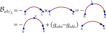
Figure 2: The second order intertwiner as a sequence of the two Darboux displacements; second line corresponds to a change $\lambda\rightarrow\nu$ of the virtual parameter (3.12).

Intertwining operators of the first and the second order allow us to construct a nontrivial integral for Lamé system $H_{a}$,

$$\mathcal{P}_{a}=\mathcal{D}_{ab}\mathcal{Y}_{ba}+\varepsilon_{ab}\mathcal{C}_{ab}=\mathcal{Y}_{ab}\mathcal{D}_{ba}-\varepsilon_{ab}\mathcal{C}_{ab}\,,$$ (3.13)

$[\mathcal{P}_{a},H_{a}]=0$, where $\mathcal{P}_{a}=\mathcal{P}(x+\tau_{a})$, $\mathcal{C}_{ab}=\mathcal{C}(\tau_{ab})=-\mathcal{C}_{ba}$, $\mathcal{C}(\tau)\equiv g(\tau,\frac{1}{2}{\rm\bf K})=\mathrm{dn}\,2\tau/(\mathrm{sn}\,2\tau\mathrm{cn}\,2\tau)$. Integral (3.13) is nothing else as the Lax operator for one-gap Lamé system (2.2), whose explicit form is

$$\mathcal{P}(x)=\frac{d^{3}}{dx^{3}}+(1+k^{2}-3k^{2}\mathrm{sn}^{2}x)\frac{d}{dx}-3k^{2}\mathrm{sn}\,x\mathrm{cn}\,x\mathrm{dn}\,x\,,\qquad\mathcal{P}^{\dagger}=-\mathcal{P}\,.$$ (3.14)

Relation (3.13) can be presented in the equivalent form

$$\mathcal{D}_{ab}\mathcal{D}_{bc}\mathcal{D}_{ca}=\mathcal{P}_{a}-g_{abc}H_{a}+\varepsilon_{ab}-\xi_{abc}\,,$$ (3.15)

where

$$\xi_{abc}\equiv\varepsilon_{ab}(g_{abc}-\mathcal{C}_{ab})\,.$$ (3.16)

Making use of the equivalent representation for the function (2.11), (2.12),

$$g(\tau;\mu)=\frac{\mathcal{C}(\tau)\varepsilon(\tau)-\mathcal{C}(\mu)\varepsilon(\mu)}{\varepsilon(\tau)-\varepsilon(\mu)}\,,$$

one can check that the three-index object defined in (3.16) possesses the same antisymmetry properties as $g_{abc}$, $\xi_{abc}=-\xi_{bac}=-\xi_{acb}$. We can also write

$$\mathcal{P}_{a}=-\mathcal{B}_{ab/c}\mathcal{D}_{ba}+g_{abc}H_{a}+\xi_{abc}=-\mathcal{D}_{ab}\mathcal{B}_{ba/c}-g_{abc}H_{a}-\xi_{abc}\,,$$ (3.17)

see Fig. 3. With the help of (3.17) and relations

$$\varepsilon_{ab}\varepsilon_{bc}\varepsilon_{ca}-\xi_{abc}^{2} = 0,$$

$$\varepsilon_{ab}\varepsilon_{ac}+\varepsilon_{ab}\varepsilon_{bc}+\varepsilon_{ac}\varepsilon_{bc}-2g_{abc}\xi_{abc} = k^{\prime}{}^{2},$$

$$\varepsilon_{ab}+\varepsilon_{ac}+\varepsilon_{bc}-g^{2}_{abc} = -(1+k^{\prime}{}^{2})\,,$$ (3.18)

we find that the Lax integral and the Hamiltonian satisfy the Burchnall-Chaundy operator identity

$$-\mathcal{P}^{2}=P(H)\,,\qquad P(H)=H(H-k^{\prime}{}^{2})(H-1)\,,$$ (3.19)

where $P(H)$ is a spectral polynomial of the one-gap Lamé system (2.2). One can show that in correspondence with (3.19), the physical states (2.3) are also the eigenstates of the Lax operator, $\mathcal{P}\Psi^{\alpha}_{\pm}(x)=\mp i\eta(E(\alpha))\sqrt{P(E(\alpha))}$, where $\eta(E)=-1$ for the valence and $+1$ for the conduction bands [22]. The Lax integral distinguishes the left- ($\Psi^{\alpha}_{+}$) and the right- ($\Psi^{\alpha}_{-}$) moving Bloch modes inside these bands, and annihilates the band-edge states.

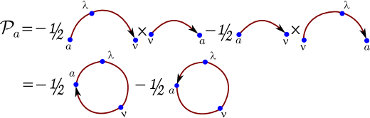
Figure 3: Two representations for the third order (Lax) integral: $\mathcal{P}_{a}=-\frac{1}{2}\mathcal{D}_{a\nu}\mathcal{B}_{\nu a/\lambda}-\frac{1}{2}\mathcal{B}_{a\nu/\lambda}\mathcal{D}_{\nu a}=-\frac{1}{2}\mathcal{D}_{a\nu}\mathcal{D}_{\nu\lambda}\mathcal{D}_{\lambda a}-\frac{1}{2}\mathcal{D}_{a\lambda}\mathcal{D}_{\lambda\nu}\mathcal{D}_{\nu a}$.

Proceeding from the definition of the second order operator $\mathcal{B}_{ab/\lambda}$ as a composition of the first order Darboux displacement generators, one can generalize the picture by treating the intermediate system $H_{\lambda}$ not just as a virtual one but on equal grounds as the systems $H_{a}$ and $H_{b}$.

The second order intertwining generator can be generalized for the case of the third order. Making use of the already known lower order relations and identity (3.12), one finds

$$\mathcal{D}_{ab}\mathcal{D}_{bc}\mathcal{D}_{cd}=-\mathcal{B}_{ac/b}\mathcal{D}_{cd}=-\mathcal{D}_{ab}\mathcal{B}_{bd/c}$$

$$=-(H_{a}+\varepsilon_{dc})\mathcal{D}_{ad}+(g_{acd}-g_{acb})\mathcal{B}_{ad/c}=-(H_{a}+\varepsilon_{ab})\mathcal{D}_{ad}+(g_{bda}-g_{bdc})\mathcal{B}_{ad/b}\,.\qquad\quad$$ (3.20)

The variation in the form of the two last expressions is in the intermediate indices. Such an ambiguity (freedom) related to the intermediate indices also appears in the higher order generalizations of the intertwining relations and integrals (Darboux loops). If we put $d=a$ in (3.20), the triple product of the $\mathcal{D}$s reduces to a third order Darboux loop (3.15), while in the two last expressions the first order operator $\mathcal{D}$ and the coefficient before the second order intertwining operator are singular. A careful treatment of these expressions in the limit sense $d\rightarrow a$ reproduces correctly the r.h.s. of the relation (3.15).

In the next, the fourth order case, we get in the same way

$$\mathcal{D}_{ab}\mathcal{D}_{bc}\mathcal{D}_{cd}\mathcal{D}_{df} = \mathcal{B}_{ac/b}\mathcal{B}_{cf/d}=(H_{a}+\varepsilon_{dc}+g_{adc}-g_{adf})\mathcal{B}_{af/d}$$ (3.21)

$$+ (g_{acd}-g_{acb})(H_{a}+\varepsilon_{fd})\mathcal{D}_{af}.$$

Taking in the last relation $f=a$, we find that the fourth order integral for $H_{a}$ can be presented as follows

$$\mathcal{D}_{ab}\mathcal{D}_{bc}\mathcal{D}_{cd}\mathcal{D}_{da}=(H_{a}+\varepsilon_{dc})(H_{a}+\varepsilon_{ad})+(g_{acb}-g_{acd})(\mathcal{P}_{a}+g_{acd}H_{a}+\xi_{acd})\,,$$ (3.22)

i.e. it reduces to a function of $H_{a}$ and $\mathcal{P}_{a}$. Continuing, we find that in the general case the closed (loop) sequence of the $n$ Darboux transformations $\mathcal{D}_{ab_{1}}\mathcal{D}_{b_{1}b_{2}}\ldots\mathcal{D}_{b_{n-1}a}$ is an integral of motion for the system $H_{a}$ of the form

$$\mathcal{D}_{ab_{1}}\mathcal{D}_{b_{1}b_{2}}\ldots\mathcal{D}_{b_{n-1}a}=h_{1}(H_{a})+h_{2}(H_{a})\mathcal{P}_{a}\,,$$ (3.23)

where $h_{1,2}(H_{a})$ are certain polynomials of $H_{a}$. An unclosed sequence of $n$ Darboux transformations reduces, analogously, to a combination of the first and the second order intertwining operators with coefficients to be some functions of the intertwined Hamiltonians $H_{a}$ and $H_{c}$,

$$\mathcal{D}_{ab_{1}}\mathcal{D}_{b_{1}b_{2}}\ldots\mathcal{D}_{b_{n-1}c}=f_{1}(H_{a})\mathcal{D}_{ac}+f_{2}(H_{a})\mathcal{B}_{ac/b_{n-1}}=\mathcal{D}_{ac}f_{1}(H_{c})+\mathcal{B}_{ac/b_{n-1}}f_{2}(H_{c})\,.$$ (3.24)

Index $b_{n-1}$ in $\mathcal{B}_{ac/b_{n-1}}$ can be changed for any other intermediate index by employing identity (3.12).

We conclude therefore that the higher order open chains of the Darboux displacement transformations reduce as differential operators to linear combinations of the two basic blocks: the first, $\mathcal{D}$, and the second, $\mathcal{B}$, order Darboux displacement generators with coefficients to be certain functions of the intertwined Hamiltonians. In the case of the closed (loop) chains, they reduce, analogously, to a linear function of the third order Lax integral $\mathcal{P}$ with coefficients depending on the Hamiltonian. No new structures do appear in addition to these sets of the first and the second order intertwining generators and the third order Lax integrals, which will play a role of the basic blocks in the associated supersymmetric construction, to the discussion of which we pass over in the next section.

4 Supersymmetry of self-isospectral periodic chains

In this section we introduce a kind of the $N$-extended system to be a self-isospectral chain of one-gap Lamé systems, and study general characteristics of the supersymmetric structure associated with it.

Consider a chain of $N\geq 2$ one-gap Lamé systems which we describe by a matrix Hamiltonian

$$\mathcal{H}=diag(H_{1},\ldots,H_{N})\,.$$ (4.1)

Here we use the same notations as in (3.4), $H_{a}=H(x+\tau_{a})$, $a=1,\ldots,N$, and assume that the set of the shift parameters $\tau_{a}$ is restricted by the condition $\tau_{ab}=\frac{1}{2}(\tau_{b}-\tau_{a})\neq n{\rm\bf K}$ for any pair of indices $a\neq b$, i.e. we suppose that the arguments of Hamiltonians of any two subsystems are shifted mutually for any distance to be different from the real period $n2{\rm\bf K}$.

Introduce a symbol ${\hat{e}}_{ab}$ defined by ${\hat{e}}_{ab}=+1$ for $a<b$, ${\hat{e}}_{ab}=-1$ for $a>b$, and ${\hat{e}}_{ab}=0$ if $a=b$. We imply that $({\hat{e}}_{ab})^{2n+1}={\hat{e}}_{ab}$, $n\in\mathbb{Z}$, while $({\hat{e}}_{ab})^{2n}=+1$ for $a\neq b$ and $({\hat{e}}_{ab})^{2n}=0$ for $a=b$. We also introduce the $N\times N$ matrices:

$$\left({\Sigma}_{1}^{ab}\right)_{ij}=({\hat{e}}_{ab})^{2}(\delta_{i}^{a}\delta_{j}^{b}+\delta_{i}^{b}\delta_{j}^{a})\,,\qquad\left({\Sigma}_{2}^{ab}\right)_{ij}={\mathbf{i}}{\hat{e}}_{ab}(\delta_{i}^{a}\delta_{j}^{b}-\delta_{i}^{b}\delta_{j}^{a})\,,$$ (4.2)

$$\left({\Sigma}_{3}^{ab}\right)_{ij}={\hat{e}}_{ab}(\delta_{i}^{a}\delta_{j}^{a}-\delta_{i}^{b}\delta_{j}^{b})\,,\qquad\left({\mathbb{I}}^{ab}\right)_{ij}=({\hat{e}}_{ab})^{2}(\delta_{i}^{a}\delta_{j}^{a}+\delta_{i}^{b}\delta_{j}^{b})\,.$$ (4.3)

In (4.2) and (4.3) we assume that $a\neq b$, and so, the first factor in definition of $\Sigma_{1}^{ab}$ and ${\mathbb{I}}^{ab}$ can be omitted. By definition, all the four matrices are symmetric in indices $a,b$, ${\Sigma}_{k}^{ab}={\Sigma}_{k}^{ba}$, $k=1,2,3$, ${\mathbb{I}}^{ab}={\mathbb{I}}^{ba}$. For $N=2$ they reduce to the three Pauli and the unit matrices, and for $N\geq 2$ satisfy the same algebra ${\Sigma}_{i}^{ab}{\Sigma}_{j}^{ab}=\delta_{ij}{\mathbb{I}}^{ab}+{\mathbf{i}}\epsilon_{ijk}{\Sigma}_{k}^{ab}$, $i,j,k=1,2,3$.

Making use of the intertwining relations from the previous section, we find that the system (4.1) is characterized by the $N(N-1)$ nontrivial integrals

$$\left(S^{ab}_{l}\right)_{ij}=({\mathbf{i}})^{l+1}\left({\Sigma}_{1}^{ab}\right)_{ij}({\hat{e}}_{ij})^{l}{{\mathcal{D}}}_{ij}\,,\qquad l=1,2\,,$$ (4.4)

which are the matrix differential operators of the first order, and by the same number of the integrals of the second order

$$\left(Q^{ab}_{l/\lambda}\right)_{ij}=(\delta_{i}^{a}\delta_{j}^{b}+\delta_{i}^{b}\delta_{j}^{a})({\mathbf{i}}{\hat{e}}_{ij})^{l-1}{{\mathcal{B}}}_{ij/\lambda}\,,\qquad l=1,2\,,$$ (4.5)

$$[{\mathcal{H}},S_{l}^{ab}]=0,\qquad[{\mathcal{H}},Q_{l/\lambda}^{ab}]=0\,.$$ (4.6)

In definition of the integrals (4.5) we suppose that the virtual parameter $\tau_{\lambda}$ can take independent values for each pair of indices $a\neq b$, and for any of the two values of the index $l$; the only restriction, as before, is $\tau_{a\lambda},\tau_{\lambda b}\neq n{\rm\bf K}$. On the other hand, relation (3.12) means that any second order integral $Q$ with the changed value of the virtual parameter is a linear combination of the initial operator $Q$ and of the first order integral $S$.

In accordance with the introduced notations, the integrals with the indices $l=1$ and $l=2$ are related by

$$S^{ab}_{2}={\mathbf{i}}{\Sigma}_{3}^{ab}S^{ab}_{1},\qquad Q^{ab}_{2/\lambda}={\mathbf{i}}{\Sigma}_{3}^{ab}Q^{ab}_{1/\lambda}\,.$$ (4.7)

This is coherent with the fact that ${\mathbb{I}}^{ab}$ and ${\Sigma}_{3}^{ab}$ are also the integrals of motion for ${\mathcal{H}}$, $[{\mathcal{H}},{\mathbb{I}}^{ab}]=[{\mathcal{H}},{\Sigma}_{3}^{ab}]=0$, and they act, respectively, as the identity and $\sigma_{3}=diag(1,-1)$ matrices in the two-term subsystem specified by the indices $a\neq b$. Also, the following relations are valid:

$$M^{ab}=M^{ba},\qquad M^{ab}W^{cd}=0\quad{\rm when\,\,all\,}\,a,b,c,d\,\,{\rm are\,\,distinct}\,,$$ (4.8)

where any of $M$ and $W$ is $S_{l}$ or $Q_{l/\lambda}$.

Matrix

$$\Gamma=diag(1,-1,\ldots,(-1)^{N-1},(-1)^{N})\,,\qquad\Gamma^{2}=1\,,$$ (4.9)

is an (zero order) integral of motion for the system (4.1), $[\mathcal{H},\Gamma]=0$, and can be taken as a grading operator. It identifies the integrals $S_{l}^{ab}$ and $Q_{l/\lambda}^{ab}$ with $a-b=2n+1$ as fermionic operators, $\{\Gamma,M^{ab}\}=0$, and those with $a-b=2n$ as bosonic, $[\Gamma,M^{ab}]=0$. To identify the superalgebraic structure generated by the integrals of motion, we compute anti-commutators between fermionic integrals (supercharges), and we take commutators between bosonic, and between bosonic and fermionic integrals. In accordance with (4.8), corresponding commutators, $[M^{ab},M^{cd}]$, and anti-commutators, $\{M^{ab},M^{cd}\}$, take zero values when all the indices $a,b,c,d$ are distinct. Nontrivial anti-commutators for fermionic supercharges are

$$\{S^{ab}_{l},S^{ab}_{m}\}=2\delta_{lm}{\mathbb{I}}^{ab}({\mathcal{H}}+\varepsilon_{ab})\,,$$ (4.10)

$$\{S^{ab}_{l},S^{bc}_{m}\}=({\hat{e}}_{ab})^{l}({\hat{e}}_{bc})^{m}\left(\delta_{lm}(-1)^{l}Q^{ac}_{1/b}+(1-\delta_{lm}){\hat{e}}_{ac}Q^{ac}_{2/b}\right)\,,$$ (4.11)

$$\{Q^{ab}_{l/\lambda},Q^{ab}_{m/\lambda}\}=2\delta_{lm}{\mathbb{I}}^{ab}({\mathcal{H}}+\varepsilon_{a\lambda})({\mathcal{H}}+\varepsilon_{b\lambda})\,,$$ (4.12)

$$\{Q^{ab}_{l/\lambda},Q^{bc}_{m/\lambda}\}=({\hat{e}}_{ab})^{l-1}({\hat{e}}_{bc})^{m-1}\left(\delta_{lm}(-1)^{l-1}Q^{ac}_{1/\lambda}+(1-\delta_{lm}){\hat{e}}_{ac}Q^{ac}_{2/\lambda}\right)({\mathcal{H}}+\varepsilon_{b\lambda})\,,$$ (4.13)

$$\{Q^{ab}_{l/\lambda},S^{ab}_{m}\}=2({\hat{e}}_{ab})^{l-1}({\hat{e}}_{ba})^{m}{\mathbb{I}}^{ab}\left(\delta_{lm}(-1)^{l}(g_{ab\lambda}{\mathcal{H}}+\xi_{ab\lambda})-(1-\delta_{lm})L\right)\,,$$ (4.14)

$$\{Q^{ab}_{l/\lambda},S^{bc}_{m}\}=({\hat{e}}_{ab})^{l-1}({\hat{e}}_{bc})^{m}\left(\delta_{lm}(-1)^{l+1}{\hat{e}}_{ac}S^{ac}_{1}+(1-\delta_{lm})S^{ac}_{2}\right)({\mathcal{H}}+\varepsilon_{bc})\,.$$ (4.15)

The nontrivial commutators are given by

$$[S^{ab}_{l},S^{ab}_{m}]=-2{\mathbf{i}}({\hat{e}}_{ab})^{l+1}({\hat{e}}_{ba})^{m}(1-\delta_{lm}){\Sigma}_{3}^{ab}({\mathcal{H}}+\varepsilon_{ab})\,,$$ (4.16)

$$[S^{ab}_{l},S^{bc}_{m}]={\mathbf{i}}({\hat{e}}_{ab})^{l}({\hat{e}}_{bc})^{m}\left(\delta_{lm}(-1)^{l+1}{\hat{e}}_{ac}Q^{ac}_{2/b}-(1-\delta_{lm})Q^{ac}_{1/b}\right)\,,$$ (4.17)

$$[Q^{ab}_{l/\lambda},Q^{ab}_{m/\lambda}]=-2{\mathbf{i}}({\hat{e}}_{ab})^{l}({\hat{e}}_{ba})^{m-1}(1-\delta_{lm}){\Sigma}_{3}^{ab}({\mathcal{H}}+\varepsilon_{a\lambda})({\mathcal{H}}+\varepsilon_{b\lambda})\,,$$ (4.18)

$$[Q^{ab}_{l/\lambda},Q^{bc}_{m/\lambda}]={\mathbf{i}}({\hat{e}}_{ab})^{l-1}({\hat{e}}_{bc})^{m-1}\left(\delta_{lm}(-1)^{l}{\hat{e}}_{ac}Q^{ac}_{2/\lambda}+(1-\delta_{lm})Q^{ac}_{1/\lambda}\right)({\mathcal{H}}+\varepsilon_{b\lambda})\,,$$ (4.19)

$$[Q^{ab}_{l/\lambda},S^{ab}_{m}]=2{\mathbf{i}}({\hat{e}}_{ab})^{l}({\tilde{\epsilon}}_{ba})^{m}{\Sigma}_{3}^{ab}\left((-1)^{l+1}\delta_{lm}L+(1-\delta_{lm})(g_{ab\lambda}{\mathcal{H}}+\xi_{ab\lambda})\right)\,,$$ (4.20)

$$[Q^{ab}_{l/\lambda},S^{bc}_{m}]={\mathbf{i}}({\hat{e}}_{ab})^{l-1}({\hat{e}}_{bc})^{m}\left(\delta_{lm}(-1)^{l}S^{ac}_{2}+(1-\delta_{lm}){\hat{e}}_{ac}S^{ac}_{1}\right)({\mathcal{H}}+\varepsilon_{bc})\,.$$ (4.21)

In correspondence with the comment on the change of the virtual index we made above, without loss of generality we put the same value for it in both second order integrals in each of the corresponding (anti)-commutators in (4.12), (4.13), (4.18) and (4.19).

In (4.14) and (4.20) there appears a nontrivial matrix operator

$$L=-{\mathbf{i}}\,diag(\mathcal{P}_{1},\mathcal{P}_{2},\cdots,\mathcal{P}_{N})\,,$$ (4.22)

composed from the third order Lax operators $\mathcal{P}_{a}=\mathcal{P}(x+\tau_{a})=-{\scriptstyle{\frac{1}{2}}}({{\mathcal{D}}}_{ab}{{\mathcal{B}}}_{ba/\lambda}+{{\mathcal{B}}}_{ab/\lambda}{{\mathcal{D}}}_{ba})$, see Eq. (3.13). The bosonic integral $L$ is a central element of the superalgebra with the grading operator $\Gamma$,

$$[L,{\mathcal{H}}]=[\Gamma,L]=0,\qquad[L,S_{l}^{ab}]=[L,Q_{l/\lambda}^{ab}]=0\,.$$ (4.23)

For the self-isospectral chain system (4.1), we have $N$ obvious (bosonic for (4.9)) third order integrals $L^{a}=-{\mathbf{i}}\,diag(0,\ldots,0,\mathcal{P}_{a},0,\ldots,0)$, the sum of which corresponds to the central element $L$. To write the commutation relations for them in the general case of the $N$-terms chain, it is convenient to define the linear combinations of $L^{a}$, $L^{ab}_{1}={\mathbb{I}}^{ab}L$ and $L^{ab}_{2}={\Sigma}_{3}^{ab}L$, remembering that for $N>2$ not all them are linearly independent. All these third order integrals commute between themselves, while their nontrivial commutators with the first and the second order integrals are

$$[L^{ab}_{l},S^{ab}_{m}]=2{\mathbf{i}}^{m}({\hat{e}}_{ab})^{m+1}\delta_{l2}({\Sigma}_{3}^{ab})^{m+1}[LS]^{ab}\,,$$ (4.24)

$$[L^{ab}_{l},S^{bc}_{m}]={\mathbf{i}}^{m}({\hat{e}}_{ba})^{l-1}{\hat{e}}_{bc}({\Sigma}_{3}^{bc})^{m+1}[LS]^{bc}\,,$$ (4.25)

$$[L^{ab}_{l},Q^{ab}_{m/\lambda}]=-2{\mathbf{i}}^{m}\delta_{l2}({\Sigma}_{3}^{ab})^{m}[LQ]^{ab}_{/\lambda}\,,$$ (4.26)

$$[L^{ab}_{l},Q^{bc}_{m/\lambda}]=-{\mathbf{i}}^{m+1}({\hat{e}}_{ba})^{l-1}{\hat{e}}_{bc}({\Sigma}_{3}^{bc})^{m}[LQ]^{bc}_{/\lambda}\,,$$ (4.27)

where $l=1,2$, and we denote

$$[LS]^{ab}\equiv Q^{ab}_{1/\lambda}({\mathcal{H}}+\varepsilon_{ab})-{\hat{e}}_{ab}S^{ab}_{1}(g_{ab\lambda}{\mathcal{H}}+\xi_{ab\lambda})\,,$$ (4.28)

$$[LQ]^{ab}_{/\lambda}\equiv{\hat{e}}_{ab}Q^{ab}_{2/\lambda}(g_{ab\lambda}{\mathcal{H}}+\xi_{ab\lambda})+S^{ab}_{2}\big{(}{\mathcal{H}}({\mathcal{H}}+2k^{\prime 2}\varepsilon_{ab}^{-1}-\varepsilon_{a\lambda}-\varepsilon_{b\lambda})+\varepsilon_{a\lambda}\varepsilon_{b\lambda}\big{)}\,.$$ (4.29)

Though on the right hand side of (4.28), there appears explicitly a virtual parameter $\lambda$, the complete combination of the integrals there does not depend on $\lambda$. This can be checked by making use of definitions (4.4), (4.5) and Eqs. (3.9) and (3.16).

We see that the set of the first, the second and the third order integrals of motion, which are Hermitian matrix operators, generate a kind of nonlinear superalgebra. A nonlinearity is related to the fact that some of the (anti)-commutators of these integrals are quadratic in the Hamiltonian $\mathcal{H}$, or include $\mathcal{H}$ or $\mathcal{H}^{2}$ as a multiplier at other integrals. The results on the general form of intertwining relations from the previous section show that no new independent integrals do appear in addition to those we already found. The interesting property of this supersymmetric structure is also that the set of the second order integrals $Q^{ab}_{l/\lambda}$ taken with the same value for the virtual parameter $\lambda$ (i.e. with the same shift parameter $\tau_{\lambda}$) together with the Hamiltonian $\mathcal{H}$ form a closed nonlinear sub-superalgebra, see Eqs. (4.12), 4.13), (4.18) and (4.19). The second order integrals can be reduced to a ‘standard’ form with a prescribed, (any) fixed value of the virtual parameter by means of relation (3.12).

5 Alternative choices for the $\mathbb{Z}_{2}$-grading operator

The choice (4.9) for the grading operator is not unique. The permutation of diagonal elements in (4.9), or multiplication of some of them by $-1$ changes the identification of integrals as fermionic and bosonic ones, and, as a consequence, some commutation relations will be changed for anti-commutation relations and vice versa. This does not change, however, the bosonic nature of the diagonal matrix integrals $L^{ab}_{l}$, and a global conclusion on a nonlinear nature of superalgebra.

There are alternative choices for the grading operator which involve reflections in the coordinate $x$ and in the shift parameters. They provide some new features for the superalgebraic structure. Let us discuss some of such alternatives. Consider the reflection in $x$ (parity) operator $\mathcal{R}$, $\mathcal{R}x=-x\mathcal{R}$, $\mathcal{R}\tau_{i}=\tau_{i}\mathcal{R}$, $\mathcal{R}^{2}=1$, and the operator $\mathcal{T}$ that reflects any of the shift parameters, including the virtual ones, $\mathcal{T}\tau_{i}=-\tau_{i}\mathcal{T}$, $\mathcal{T}x=x\mathcal{T}$, $\mathcal{T}^{2}=1$, and commutes with $\mathcal{R}$. The product of these two operators is a nontrivial, nonlocal integral of motion for our chain system, $[\mathcal{RT},\mathcal{H}]=0$, and its square equals $1$. So, it can be identified as another sort of the grading operator,

$$\hat{\Gamma}=\mathcal{RT}\,.$$ (5.1)

The operator $\hat{\Gamma}$ anti-commutes with all the first, $S^{ab}_{l}$, and the third, $L^{ab}_{l}$, order integrals, and commutes with the second order integrals $Q^{ab}_{l/\lambda}$. In this case $S^{ab}_{l}$ and $L^{ab}_{l}$ are the fermionic operators, while $Q^{ab}_{l/\lambda}$ are the bosonic ones. To compute the superalgebraic structure for such a choice of the grading operator, we have to use coherently with the described identification of bosonic and fermionic generators the corresponding (anti)-commutators from the previous section, which should be supplied with the nontrivial anti-commutation relations that involve the third order integrals,

$$\{L^{ab}_{l},S^{ab}_{m}\}=2{\mathbf{i}}^{m}({\hat{e}}_{ab})^{m+1}\delta_{l1}({\Sigma}_{3}^{ab})^{m}[LS]^{ab}\,,$$ (5.2)

$$\{L^{ab}_{l},S^{bc}_{m}\}={\mathbf{i}}^{m}({\hat{e}}_{ba})^{l-1}({\Sigma}_{3}^{bc})^{m}[LS]^{bc}\,,$$ (5.3)

$$\{L^{ab}_{l},Q^{ab}_{m/\lambda}\}=-2{\mathbf{i}}^{m}\delta_{l1}({\Sigma}_{3}^{ab})^{m+1}[LQ]^{ab}_{/\lambda}\,,$$ (5.4)

$$\{L^{ab}_{l},Q^{bc}_{m/\lambda}\}=-{\mathbf{i}}^{m+1}({\hat{e}}_{ba})^{l-1}({\Sigma}_{3}^{bc})^{m+1}[LQ]^{bc}_{/\lambda}\,,$$ (5.5)

$$\{L^{ab}_{l},L^{ab}_{m}\}=2({\Sigma}_{3}^{ab})^{l+m}P(\mathcal{H})\,,$$ (5.6)

$$\{L^{ab}_{l},L^{bc}_{m}\}=({\mathbb{I}}^{ab}-\hat{e}_{ab}\Sigma_{3}^{ab})({\hat{e}}_{ba})^{l-1}({\hat{e}}_{bc})^{m-1}P(\mathcal{H})\,.$$ (5.7)

Under such a choice of the grading operator, the spectral polynomial of the chain, $P(\mathcal{H})=\mathcal{H}(\mathcal{H}-k^{\prime}{}^{2})(\mathcal{H}-1)$, appears explicitly in the superalgebraic structure. This choice, therefore, is coherent with the structure of a hidden, bosonized supersymmetry (1.1) [12] that is present in each of the chain subsystems $H_{a}$ [4]. The relation (5.6) particularly reveals the property of the Lax operators that is essential for physical applications: each third order differential operator $L_{l}$ here is an annihilator of the three band edge states in the spectrum of the corresponding chain Lamé subsystem $H_{l}$, see refs. [21, 22, 23] for the further details. In the case of the choice of the grading operator discussed in the previous section, this peculiarity of the Lax operators does not show up in the superalgebraic relations.

The product of the two operators, (4.9) and (5.1), can also be chosen as a grading operator. Yet other possibilities are associated with the introduction of the operators of the permutations of the displacement parameters, $T^{ab}=T^{ba}$, defined by $T^{ab}\tau_{b}=\tau_{a}T^{ab}$, $T^{ab}\tau_{c}=\tau_{c}T^{ab}$, $T^{ab}x=xT^{ab}$. Combining such operators with the matrix structures $\Sigma^{ab}_{1,2,3}$, and reflection operators $\mathcal{R}$ and $\mathcal{T}$, one can construct more integrals which can be taken as the grading operators. This does not add something essentially new to the structures we already observed, and we do not discuss these other possibilities here.

In the last section we present some further arguments in favor of necessity to consider alternative choices for the grading operator (alongside with the choice discussed in the previous section) in the context of possible physical applications.

6 Supersymmetric structure of the $N=3$ chain

In the case of the two-term chain ($N=2$), we have $a,b=1,2$. A complete set of independent integrals is formed by the two integrals of the first order, $S^{12}_{l}$, $l=1,2,$ the two integrals of the second order, $Q^{12}_{l/\lambda}$, and by the two integrals of the third order, $L^{12}_{1}=L$ and $L^{12}_{2}$. In the list of the (anti)-commutation relations of the integrals there do not appear (anti)-commutators which involve the generators with three different indices $a,b,c$. For the discussion of the case $N=2$ we refer to [22]. Here we consider in more detail the next case $N=3$ to illustrate explicit matrix form of the involved structures.

The $N=3$ Hamiltonian is

$${\mathcal{H}}=\begin{pmatrix}H_{1}&0&0\\ 0&H_{2}&0\\ 0&0&H_{3}\end{pmatrix}.$$ (6.1)

The system has six trivial matrix integrals of motion,

$${\mathbb{I}}^{12}=\begin{pmatrix}1&0&0\\ 0&1&0\\ 0&0&0\end{pmatrix},\quad{\mathbb{I}}^{13}=\begin{pmatrix}1&0&0\\ 0&0&0\\ 0&0&1\end{pmatrix},\quad{\mathbb{I}}^{23}=\begin{pmatrix}0&0&0\\ 0&1&0\\ 0&0&1\end{pmatrix},$$ (6.2)

$${\Sigma}_{3}^{12}=\begin{pmatrix}1&0&0\\ 0&-1&0\\ 0&0&0\end{pmatrix},\quad{\Sigma}_{3}^{13}=\begin{pmatrix}1&0&0\\ 0&0&0\\ 0&0&-1\end{pmatrix},\quad{\Sigma}_{3}^{23}=\begin{pmatrix}0&0&0\\ 0&1&0\\ 0&0&-1\end{pmatrix},$$ (6.3)

which appear explicitly in the superalgebraic (anti)-commutation relations. This set contains only three linearly independent matrices. Three nontrivial integrals to be the first order differential operators are

$$S^{12}_{1}=\begin{pmatrix}0&-{{\mathcal{D}}}_{12}&0\\ {{\mathcal{D}}}_{21}&0&0\\ 0&0&0\end{pmatrix},\quad S^{13}_{1}=\begin{pmatrix}0&0&-{{\mathcal{D}}}_{13}\\ 0&0&0\\ {{\mathcal{D}}}_{31}&0&0\end{pmatrix},\quad S^{23}_{1}=\begin{pmatrix}0&0&0\\ 0&0&-{{\mathcal{D}}}_{23}\\ 0&{{\mathcal{D}}}_{32}&0\end{pmatrix},$$ (6.4)

and the other three are $S^{ab}_{2}=i{\Sigma}_{3}^{ab}S^{ab}_{1}$. Six second order integrals of motion are given by

$$Q^{12}_{1/\lambda}=\begin{pmatrix}0&{{\mathcal{B}}}_{12/\lambda}&0\\ {{\mathcal{B}}}_{21/\lambda}&0&0\\ 0&0&0\end{pmatrix},\quad Q^{13}_{1/\lambda}=\begin{pmatrix}0&0&{{\mathcal{B}}}_{13/\lambda}\\ 0&0&0\\ {{\mathcal{B}}}_{31/\lambda}&0&0\end{pmatrix},\quad Q^{23}_{1/\lambda}=\begin{pmatrix}0&0&0\\ 0&0&{{\mathcal{B}}}_{23/\lambda}\\ 0&{{\mathcal{B}}}_{32/\lambda}&0\end{pmatrix},$$ (6.5)

and $Q^{ab}_{2/\lambda}=i{\Sigma}_{3}^{ab}Q^{ab}_{1/\lambda}$. Finally, the set of the three linearly independent third order integrals is

$$L^{12}=\begin{pmatrix}-{\mathbf{i}}\mathcal{P}_{1}&0&0\\ 0&-{\mathbf{i}}\mathcal{P}_{2}&0\\ 0&0&0\end{pmatrix},\quad L^{13}=\begin{pmatrix}-{\mathbf{i}}\mathcal{P}_{1}&0&0\\ 0&0&0\\ 0&0&-{\mathbf{i}}\mathcal{P}_{3}\end{pmatrix},\quad L^{23}=\begin{pmatrix}0&0&0\\ 0&-{\mathbf{i}}\mathcal{P}_{2}&0\\ 0&0&-{\mathbf{i}}\mathcal{P}_{3}\end{pmatrix}.$$ (6.6)

Their linear combination corresponds to the integral $L$, $L=\frac{1}{2}(L^{12}+L^{13}+L^{23})$.

The grading operator can be chosen in one of the forms

$$\Gamma=\begin{pmatrix}1&0&0\\ 0&-1&0\\ 0&0&1\end{pmatrix},\quad\hat{\Gamma}=\begin{pmatrix}\mathcal{RT}&0&0\\ 0&\mathcal{RT}&0\\ 0&0&\mathcal{RT}\end{pmatrix},\quad\hat{\Gamma}_{1}=\Gamma\hat{\Gamma}=\begin{pmatrix}\mathcal{RT}&0&0\\ 0&-\mathcal{RT}&0\\ 0&0&\mathcal{RT}\end{pmatrix}.$$ (6.7)

When $\Gamma$ is chosen as the grading operator, we have eight nontrivial fermionic integrals of motion $S^{12}_{l},$ $S^{23}_{l},$ $Q^{12}_{l/\lambda},$ $Q^{23}_{l/\lambda}$, and seven linear independent bosonic integrals $S^{13}_{l},$ $Q^{13}_{l/\lambda}$, and $L^{12}$, $L^{13}$ and $L^{23}$. In the case of the choice of $\hat{\Gamma}$ as the grading operator, we have nine fermionic integrals $S^{ab}_{l}$ and $L^{ab}$. The second order integrals $Q^{ab}_{l/\lambda}$ constitute the set of six bosonic integrals of motion. Finally, for $\hat{\Gamma}_{1}$, we have six bosonic integrals, $S^{12}_{l}$, $S^{23}_{l}$ and $Q^{13}_{l/\lambda}$, and nine fermionic integrals, $S^{13}_{l}$, $Q^{12}_{l/\lambda}$, $Q^{23}_{l/\lambda}$, and $L^{ab}$. We see that the complete set of local nontrivial integrals of motion separates into bosonic and fermionic generators in dependence on the choice of the grading operator.

If we start from the first order integrals $S^{12}_{l}$, $S^{23}_{l}$ and $S^{13}_{l}$, their corresponding (anti)-commutation relations (4.11) and/or (4.17) (that depends on the choice of the grading operator) generate, unlike the $N=2$ case, all the six second order integrals $Q^{ab}_{l/\lambda}$. The virtual parameter $\tau_{\lambda}$ here as well as for $N>3$ can be identified with the shift parameter $\tau_{b}$ of one of the corresponding subsystems. Each time, however, the intermediate index $\lambda$ in $Q^{ab}_{l/\lambda}$ can be changed by employing relation (3.12). Anyway, for $N\geq 2$ the second order integrals $Q^{ab}_{l/\lambda}$ are generated also via the (anti)-commutators of $S^{ab}_{l}$ with the third order integrals, see Eqs. (4.24), (4.25), (4.28), (5.2) and (5.3).

7 Self-isospectral soliton chains

Consider now the infinite period limit which produces self-isospectral non-periodic chains. It is obtained by putting $k\rightarrow 1$, when, as we noted, ${\rm\bf K}\rightarrow\infty$, $2{\mathbf{i}}{\rm\bf K}^{\prime}\rightarrow{\mathbf{i}}\pi$, and one-gap Lamé Hamiltonian (2.2) transforms into that of reflectionless Pöschl-Teller system

$$H^{PT}(x)=-\frac{d^{2}}{dx^{2}}-\frac{2}{\cosh^{2}x}+1\,.$$ (7.1)

In this limit the valence band $0\leq E\leq k^{\prime}{}^{2}$ of the Lamé system shrinks into the level $E=0$ of the unique bound state of the system (7.1) described by the wave function ${\rm sech}\,x$. To get a self-isospectral supersymmetric chain of reflectionless Pöschl-Teller systems, we have to introduce also some restrictions on the displacement parameters. Namely, it is necessary to require that all the $\tau_{a}$ which appear in the arguments of the chain Hamiltonians, $H_{a}=H(x+\tau_{a})$, should not go to infinity when $k\rightarrow 1$. By this condition we prohibit that in the chain we get in the limit, there could appear free particle systems.

In such a limit, for $x$-independent structures we get

$$\mathfrak{z}(\tau)\rightarrow\coth 2\tau\,,\qquad\mathcal{C}_{ab}\rightarrow\coth 2\tau_{ab}\,,\qquad g_{ab\lambda}\rightarrow\coth 2\tau_{ab}+\coth 2\tau_{b\lambda}+\coth 2\tau_{\lambda a}\,,$$ (7.2)

$$\varepsilon_{ab}\rightarrow{\rm csch}^{2}2\tau_{ab}\,,\qquad\xi_{ab\lambda}\rightarrow-(\coth 2\tau_{a\lambda}+\coth 2\tau_{\lambda b}){\rm csch}^{2}2\tau_{ab}\,.$$ (7.3)

For the superpotential (2.8) we have $\Delta(x;\tau)\rightarrow\Delta^{PT}(x;\tau)=\tanh(x-\tau)-\tanh(x+\tau)+\coth 2\tau$. Denoting the limit of $\Delta(x_{ab};{\tau_{ab}})$ by $\Delta_{ab}^{PT}$, we find

$$\Delta_{ab}^{PT}=-\Delta_{ba}^{PT} = \tanh(x+\tau_{a})-\tanh(x+\tau_{b})+\coth(\tau_{b}-\tau_{a})$$ (7.4)

$$= \tanh 2\tau_{ab}\tanh(x+\tau_{a})\tanh(x+\tau_{b})+{2}{{\rm csch}4\tau_{ab}}\,.$$

For the first order intertwining operator we get

$$\mathcal{D}_{ab}\rightarrow X_{ab}=\frac{d}{dx}-\Delta_{ab}^{PT}\,,\qquad X_{ab}^{\dagger}=-X_{ba}\,,$$ (7.5)

and (3.2) transforms then into

$$-X_{ab}X_{ba}=H^{PT}_{a}+{\rm csch}^{2}2\tau_{ab}\,,$$ (7.6)

where $H^{PT}_{a}=H^{PT}(x+\tau_{a})$. The limit of the second order intertwining operator (3.11) can be written in the form that includes in its structure the first order operator $A_{\tau}=\frac{d}{dx}-\tanh(x+\tau)$,

$$\mathcal{Y}_{ab} \rightarrow \frac{d^{2}}{dx^{2}}-\Delta_{ab}^{PT}\frac{d}{dx}-\tanh^{2}(x+\tau_{a})+\coth^{2}2\tau_{ab}$$ (7.7)

$$= -A_{a}A^{\dagger}_{b}-\coth 2\tau_{ab}X_{ab}\,,$$

where $A_{a}\equiv A_{\tau_{a}}$. The first term in the last expression in (7.7), unlike the $X_{ab}$ and the $x$-independent multiplier $\coth 2\tau_{ab}$ in the second term, is well defined when $\tau_{b}=\tau_{a}\Rightarrow\tau_{ab}=0$. This is so because the operator $A_{\tau}$, unlike the limit of the operator $\mathcal{D}(x;\tau)$, is regular for $\tau=0$.

Making use of Eqs. (3.9) and (7.2), for the limit of the second order intertwining operator $\mathcal{B}$ we get

$$\mathcal{B}_{ab/\lambda}\rightarrow-X_{a\lambda}X_{\lambda b}=A_{a}A^{\dagger}_{b}+(\coth 2\tau_{a\lambda}+\coth 2\tau_{\lambda b})X_{ab}\equiv B_{ab/\lambda}\,,$$ (7.8)

and find that the limit of the third order integral can be presented in terms of the introduced first order operator $A_{\tau}$,

$$\mathcal{P}_{a}\rightarrow-Z_{a}\,,\quad{\rm where}\quad Z_{a}=A_{a}\frac{d}{dx}A_{a}^{\dagger}\,.$$ (7.9)

Since the first order operator $X_{ab}$ as well as the second order operators (7.7) and (7.8) intertwine the Hamiltonians $H^{PT}_{b}$ and $H^{PT}_{a}$, the operator [30]

$$Y_{ab}=A_{a}A^{\dagger}_{b}$$ (7.10)

is also the intertwining operator, $Y_{ab}H_{b}^{PT}=H_{a}^{PT}Y_{ab}$. Operator (7.10) corresponds to the infinite limit of the virtual displacement parameter, $\tau_{\lambda}\rightarrow\infty$ (or, $\tau_{\lambda}\rightarrow-\infty$), applied to $B_{ab/\lambda}$, see Fig. 4.

The intertwiner (7.10), unlike (7.7) and (7.8), is regular for $\tau_{ab}=0$ ($\tau_{a}=\tau_{b}$), when it reduces just to $H_{a}^{PT}$,

$$Y_{aa}=A_{a}A^{\dagger}_{a}=H_{a}^{PT}.$$ (7.11)

Another product of the same operators produces (for any value of the parameter $\tau_{a}$) the free particle Hamiltonian shifted for an additive constant,

$$A^{\dagger}_{a}A_{a}=-\frac{d^{2}}{dx^{2}}+1\equiv H_{0}\,.$$ (7.12)

In accordance with (7.11) and (7.12), the first order operators $A_{a}$ and $A^{\dagger}_{a}$ intertwine the Pöschl-Teller system with a free particle, $A^{\dagger}_{a}H_{a}^{PT}=H_{0}A^{\dagger}_{a}$, $H_{a}^{PT}A_{a}=A_{a}H_{0}$. From (7.4) we find that if $\tau_{b}\rightarrow\infty$ while $\tau_{a}$ is kept to be finite, $\Delta^{PT}_{ab}$ reduces to $\tanh(x+\tau_{a})$. In such a limit, $H_{b}^{PT}$ reduces to $H_{0}$, $H_{\infty}^{PT}=H_{0}$, $X_{ab}$ transforms into $A_{a}$, while the second order operators (7.7), (7.8) and (7.10) transform into $A_{a}\frac{d}{dx}$ and linear combinations of this operator and the first order operator $A_{a}$. The second order operator we have gotten intertwines $H_{a}^{PT}$ with $H_{0}$, $A_{a}\frac{d}{dx}H_{0}=H_{a}^{PT}A_{a}\frac{d}{dx}$, but this relation produces nothing new since it is a consequence of the conservation of $\frac{d}{dx}$ for a free particle system $H_{0}$, $\frac{d}{dx}H_{0}=H_{0}\frac{d}{dx}$, and of the already known relation $H_{a}^{PT}A_{a}=A_{a}H_{0}$. On the other hand, the product of this operator with the intertwiner $A^{\dagger}_{a}$, that acts in another direction between $H_{0}$ and $H^{PT}_{a}$, shows that the Lax operator of the Pöschl-Teller system, $Z_{a}$, is nothing else as the Darboux-dressed free particle momentum [34]. From (7.8) one can get a relation which involves the first order intertwiners $A_{a}$ and $X_{ab}$, and the free particle momentum. Taking the limit $\tau_{b}\rightarrow\infty$ in both representations for $B_{ab/\lambda}$, we get the relation $A_{a}\left(\frac{d}{dx}-\coth 2\tau_{a\lambda}\right)=X_{a\lambda}A_{\lambda}\,,$ and also its conjugate, $A_{\lambda}^{\dagger}X_{\lambda a}=\left(\frac{d}{dx}+\coth 2\tau_{a\lambda}\right)A_{a}^{\dagger}.$

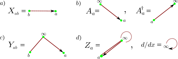
Figure 4: The first order Darboux displacement generator $X_{ab}$ translates the eigenfunctions of $H^{PT}_{b}$ into those of $H^{PT}_{a}$. The second order intertwiner $Y_{ab}$ makes the same via the virtual free particle system that is a Pöschl-Teller system translated to infinity. Lax integral $Z_{a}$ is presented as a Darboux dressed form (7.9) of the free particle integral $d/dx$.

The described limit applied to the chain (4.1) gives a non-periodic self-isospectral chain described by the Hamiltonian

$$\mathcal{H}^{PT}=diag(H_{1}^{PT},\ldots,H_{N}^{PT})\,.$$ (7.13)

The nontrivial integrals of such a system are given by the infinite period limit applied to the integrals $S^{ab}_{l}$, $Q^{ab}_{l/\lambda}$ and $L^{ab}_{l}$ by employing relations (7.5), (7.8) and (7.9). As in the periodic case, the set of the corresponding third order integrals $L^{PTab}_{l}$ contains only $N$ independent integrals. Instead of $Q^{PTab}_{l/\lambda}$, one can work with the second order matrix integrals $\mathcal{Q}^{PTab}_{l}=\lim_{\tau_{\lambda}\rightarrow\infty}Q^{PTab}_{l/\lambda}$, which are obtained by the change of ${B}_{ab/\lambda}$ for $Y_{ab}$. The corresponding superalgebra generated by these integrals, as in the periodic case, depends on the choice of the grading operator, and its concrete form can be computed by making use of the relations presented above. Again, we get a closed non-linear superalgebra, the nonlinearity of which originates from the polynomial dependence of the superalgebraic structure functions on the Hamiltonian $\mathcal{H}^{PT}$, which plays a role of the multiplicative central charge. Since we have defined $\mathcal{Q}^{PTab}_{l}$ as the $Q^{PTab}_{l/\lambda}$ taken with the same virtual parameter $\tau_{\lambda}=\infty$, the set of the second order integrals $\mathcal{Q}^{PTab}_{l}$ together with the Hamiltonian $\mathcal{H}^{PT}$ form the closed nonlinear sub-superalgebra.

If some of the displacement parameters $\tau_{a}$ are taken to be infinite, corresponding Hamiltonians $H_{a}^{PT}$ transform into those of the free particle. In this case we loose the property of the self-isospectrality of the chain, but the supersymmetric structure is still present and can also be computed by employing the relations discussed above.

8 Discussion and outlook

We investigated the unusual nonlinear supersymmetric structure of the self-isospectral crystalline chains formed by the arbitrary number $N\geq 2$ of mutually displaced periodic one-gap Lamé systems, and of the associated non-periodic self-isospectral soliton chains described by reflectionless Pöschl-Teller Hamiltonians. It is generated by the $N(N-1)$ integrals of motion which are the first order differential matrix operators, by the same number of the second order matrix integrals, and by the $N$ third order Lax integrals. The supersymmetry admits distinct choices for the grading operator, that classifies these integrals as bosonic and fermionic operators in different ways. For instance, for the example of the $N=3$ chain from Section 6, three choices of the grading operator indicated in Eq. (6.7) classify the complete set of $15$ nontrivial local integrals of motion as, respectively, $7+8=(2+2+3)+(4+4+0)$, $6+9=(0+6+0)+(6+0+3)$ and $6+9=(4+2+0)+(2+4+3)$ bosonic$+$fermionic generators, where the first, second and third numbers in each parentheses correspond to the numbers of the first, second and third order differential matrix operators. In dependence on the chosen grading operator, one of the third order integrals, $L$, is the bosonic central charge, or the fermionic supercharge to be a square root of the matrix spectral polynomial of the $N$-chain . In the latter, unlike the former, case the spectral polynomial appears explicitly just in the superalgebraic relations. This reveals the identifying characteristic of the Lax integrals: they recognize the band edge states in the spectrum of each Lamé subsystem by annihilating them. Another peculiarity is that the set of all the second order integrals of motion taken with the same virtual parameter generates together with the Hamiltonian a nonlinear sub-superalgebra.

The lowest $N$-fold degenerate energy level was chosen to be zero, and the spectra of the self-isospectral chains described by the second order matrix Hamiltonians do not depend on the values of the displacement parameters. On the other hand, according to Eqs. (4.10) and (2.10), the spectra of the first order matrix integrals $S^{ab}_{l}$ depend on the mutual shifts $\tau_{ab}$, and blow up when $\tau_{ab}$ tends to zero (modulo the period in the case of the crystalline chain). This indicates on another possibility to interpret the systems by identifying a suitable combination of the first order integrals as a Hamiltonian. For instance, for $N=2$, one can treat $S^{12}_{1}$ as the integral $\mathcal{H}_{(1)}$, or, for $N=2n$ we can choose $\mathcal{H}_{(1)}=S^{12}_{1}+S^{34}_{1}+\ldots S^{2n-1\,2n}_{1}$. The lower index indicates that the Hamiltonian is of the first order (Dirac) nature, which can be considered as a kind of Bogoliubov-de Gennes Hamiltonian in the Andreev approximation. Such $\mathcal{H}_{(1)}$ in the $N=2$ case was considered, for instance, in the physics of conducting polymers [15, 35], or as a Hamiltonian that describes the kink-antikink crystal [25, 26] (or, kink-antikink baryons in the non-periodic limit case [36]) in the Gross-Neveu model. Therefore, the $N>2$ chains in such a reinterpretation with the first order Hamiltonian would provide some generalization of the known $N=2$ models, in which spectral gaps are governed by the displacement parameters of the corresponding second order chains. The interesting peculiarity of such first order systems is that they possess the own nonlinear supersymmetry. Indeed, the operator $\hat{\Gamma}_{1}=\mathcal{RT}\Gamma$, where $\Gamma$ is given by Eq. (4.9), commutes with $\mathcal{H}_{(1)}$, and can be identified as a grading operator for such a first order system. The Lax operator $L$ anti-commutes with $\hat{\Gamma}_{1}$, and the latter classifies $\mathcal{H}_{(1)}$ and $L$ as, respectively, bosonic and fermionic generators. Since $L$ commutes with $\mathcal{H}_{(1)}$, it can be considered as a fermionic supercharge, whose square, in accordance with Eqs. (4.10) and (5.6), gives some polynomial of order six in $\mathcal{H}_{(1)}$ . For $n>1$, the system $\mathcal{H}_{(1)}$ has also other nontrivial integrals of motion, see Eq. (4.24) with $l=1$. Such a nonlinear supersymmetry in the first order system $\mathcal{H}_{(1)}$ could not be revealed, however, with the choice of the grading operator in the reflection-independent form (4.9) which identifies the Lax integral $L$ as the bosonic operator and $\mathcal{H}_{(1)}$ as the fermionic one.

Another interesting possibility for generalization of the results is to identify some linear combination of the second order matrix operators as a Hamiltonian, for instance, by taking $\mathcal{H}_{(2)}=Q^{12}_{1/\lambda}+Q^{34}_{1/\lambda}+\ldots Q^{2n-1\,2n}_{1/\lambda}$ in the case of $N=2n$. The spectrum of $\mathcal{H}_{(2)}$ like that of $\mathcal{H}_{(1)}$ depends on the shift parameters, see (4.12). For $N=2$ or $N=4$, such a second order matrix Hamiltonian has a nature to be similar to that of the Hamiltonian in the physics of bilayer graphene [37]. With respect to the grading operator $\hat{\Gamma}=\mathcal{RT}$, the Hamiltonian $\mathcal{H}_{(2)}$ and the third order operator $L$ are, respectively, the bosonic and fermionic operators. The operator $L$ as well as the operators $L^{12}_{1}$, $\ldots$, $L^{2n-1\,2n}_{1}$, see Eq. (4.26) with $l=1$, are the supercharges of the nonlinear supersymmetry of the system described by the unusual second order matrix Hamiltonian $\mathcal{H}_{(2)}$. Notice a special role played by the reflection-dependent grading operator $\hat{\Gamma}=\mathcal{RT}$ for revealing the supersymmetric structure in the indicated unusual second order system $\mathcal{H}_{(2)}$.

The peculiarity of the non-periodic case in comparison with the periodic one is that the chain subsystems can be related there, particularly, by the second order intertwiners (7.10). As the intermediate (virtual) system in this case, there appears a free particle system. The latter can be treated as the Pöschl-Teller system (7.1), $H_{\lambda}^{PT}=H_{\lambda}^{PT}(x+\tau_{\lambda})$, displaced to infinity, $\tau_{\lambda}\rightarrow\infty$. It is due to such a relation the Lax operator (7.9) has a nature of a dressed free particle momentum operator, and eigenstates of $H^{PT}$ can be obtained by the Darboux transformation of the corresponding free particle eigenstates. We have, unfortunately, no such simple relation with a free particle in the periodic case.

We considered the case of self-isospectral Hermitian chains with real displacements. The construction can be generalized for the case of complex shift parameters. The corresponding supersymmetric structure can be interesting then in the context of the physics of PT-symmetric systems [39, 40], where, again, the discrete transformation operators, particularly spatial reflection, prove to play a fundamental role [41].

Acknowledgements. The work has been partially supported by FONDECYT Grant 1095027, Chile. MP thanks the Benasque Center for Science for a stimulating environment, and University of Valladolid for hospitality during the initial stages of the work.

References

• [1] B.A. Dubrovin B.A, V.B. Matveev, S.P. Novikov, 31, 59 (1976); S. P. Novikov, S. V. Manakov, L. P. Pitaevskii and V. E. Zakharov, Theory of solitons (Plenum, New York, 1984); E. D. Belokolos, A. I. Bobenko, V. Z. Enol’skii, A. R. Its, and V. B. Matveev, Algebro- geometric approach to nonlinear integrable equations, (Springer, Berlin, 1994); F. Gesztesy, H. Holden, Soliton equations and their algebro-geometric solutions (Cambridge Univ. Press, Cambridge, 2003).
• [2] J. L. Burchnall and T. W. Chaundy, Proc. London Math. Soc. Ser. 2, 21, 420 (1923); E. L. Ince, Ordinary differential equations (Dover, 1956).
• [3] I. M. Krichever, Functional Anal. Appl. 11, 12 (1977); 12, 175 (1978); Russian Math. Surveys, 32, 185 (1977).
• [4] F. Correa and M. S. Plyushchay, Annals Phys.  322, 2493 (2007) [arXiv:hep-th/0605104]; F. Correa, L. M. Nieto and M. S. Plyushchay, Phys. Lett.  B 644, 94 (2007) [arXiv:hep-th/0608096].
• [5] A. A. Andrianov, M. V. Ioffe and V. P. Spiridonov, Phys. Lett. A 174, 273 (1993) [arXiv:hep-th/9303005].
• [6] V. A. Rubakov and V. P. Spiridonov, Mod. Phys. Lett.  A 3, 1337 (1988).
• [7] A. A. Andrianov, M. V. Ioffe and D. N. Nishnianidze, Phys. Lett.  A 201, 103 (1995) [arXiv:hep-th/9404120].
• [8] V.G. Bagrov, and B.F. Samsonov, Theor. Math. Phys. 104, 1051 (1995).
• [9] D. J. Fernandez C, Int. J. Mod. Phys.  A 12, 171 (1997) [arXiv:quant-ph/9609009].
• [10] S. M. Klishevich and M. S. Plyushchay, Nucl. Phys.  B 606, 583 (2001) [arXiv:hep-th/0012023].
• [11] V. B. Matveev and M. A. Salle, Darboux Transformations and Solitons, (Springer, Berlin, 1991).
• [12] M. S. Plyushchay, Annals Phys.  245, 339 (1996) [arXiv:hep-th/9601116]; Int. J. Mod. Phys. A 15, 3679 (2000) [arXiv:hep-th/9903130].
• [13] V. Jakubsky, L. -M. Nieto and M. S. Plyushchay, Phys. Lett. B 692, 51 (2010) [arXiv:1004.5489 [hep-th]].
• [14] H. W. Braden and A. J. Macfarlane, J. Phys. A 18, 3151 (1985).
• [15] A. Saxena and A. R. Bishop, Phys. Rev. A 44, R2251 (1991).
• [16] A.P. Veselov, A.B. Shabat, Funct. Anal. Appl. 27, 81 (1993).
• [17] G. V. Dunne and J. Feinberg, Phys. Rev.  D 57, 1271 (1998) [arXiv:hep-th/9706012].
• [18] D. J. Fernandez, J. Negro and L. M. Nieto, Phys. Lett.  A 275, 338 (2000).
• [19] D. J. Fernandez, B. Mielnik, O. Rosas-Ortiz and B. F. Samsonov, Phys. Lett.  A 294, 168 (2002) [arXiv:quant-ph/0302204].
• [20] A. A. Andrianov and A. V. Sokolov, Nucl. Phys.  B 660, 25 (2003); [arXiv:hep-th/0301062]; SIGMA 5, 064 (2009) [arXiv:0906.0549 [hep-th]].
• [21] F. Correa, V. Jakubsky, L. M. Nieto and M. S. Plyushchay, Phys. Rev. Lett.  101, 030403 (2008) [arXiv:0801.1671 [hep-th]].
• [22] M. S. Plyushchay, A. Arancibia and L. M. Nieto, Phys. Rev.  D 83, 065025 (2011) [arXiv:1012.4529 [hep-th]].
• [23] F. Correa, V. Jakubsky and M. S. Plyushchay, J. Phys. A 41, 485303 (2008) [arXiv:0806.1614 [hep-th]].
• [24] D. J. Gross and A. Neveu, Phys. Rev.  D 10, 3235 (1974).
• [25] M. Thies and K. Urlichs, Phys. Rev.  D 67, 125015 (2003) [arXiv:hep-th/0302092]; M. Thies, Phys. Rev.  D 69, 067703 (2004) [arXiv:hep-th/0308164]; O. Schnetz, M. Thies and K. Urlichs, Annals Phys.  321, 2604 (2006) [arXiv:hep-th/0511206].
• [26] G. Basar and G. V. Dunne, Phys. Rev.  D 78, 065022 (2008) [arXiv:0806.2659 [hep-th]]; G. Basar, G. V. Dunne and M. Thies, Phys. Rev.  D 79, 105012 (2009) [arXiv:0903.1868 [hep-th]].
• [27] D. Ebert and K. G. Klimenko, Phys. Rev.  D 80, 125013 (2009) [arXiv:0911.1944 [hep-ph]]; D. Ebert, N. V. Gubina, K. G. Klimenko, S. G. Kurbanov and V. C. Zhukovsky, Phys. Rev.  D 84, 025004 (2011) [arXiv:1102.4079 [hep-ph]].
• [28] S. Carignano, D. Nickel and M. Buballa, Phys. Rev.  D 82, 054009 (2010) [arXiv:1007.1397 [hep-ph]].
• [29] R. F. Dashen, B. Hasslacher and A. Neveu, Phys. Rev.  D 12, 2443 (1975).
• [30] M. S. Plyushchay and L. M. Nieto, Phys. Rev.  D 82, 065022 (2010) [arXiv:1007.1962 [hep-th]].
• [31] D.J. Gross, in : Methods in Field Theory, Les-Houches session XXVIII 1975, R. Balian and J. Zinn-Justin (Eds.), (North Holland, Amsterdam, 1976); A. Klein, Phys. Rev. D 14, 558 (1976); J. Feinberg, Phys. Rev.  D 51, 4503 (1995).
• [32] E. T. Whittaker and G. N. Watson, A Course of Modern Analysis (Cambridge Univ. Press, 1980).
• [33] D. K. Lawden, Elliptic functions and applications (Springer-Verlag New York Inc., 2010).
• [34] F. Correa, V. Jakubsky and M. S. Plyushchay, Annals Phys.  324, 1078 (2009) [arXiv:0809.2854 [hep-th]].
• [35] M. Thies and K. Urlichs, Phys. Rev.  D 72, 105008 (2005) [arXiv:hep-th/0505024]; M. Thies, J. Phys. A 39, 12707 (2006) [arXiv:hep-th/0601049].
• [36] J. Feinberg and A. Zee, Phys. Rev.  D 56, 5050 (1997) [arXiv:cond-mat/9603173]; J. Feinberg, Annals Phys. (NY)  309, 166 (2004) [arXiv:hep-th/0305240].
• [37] M. I. Katsnelson, K. S. Novoselov, and A. K. Geim, Nature Physics 2, 620 (2006).
• [38] V. Jakubsky and M. S. Plyushchay, Phys. Rev.  D 85, 045035 (2012) [arXiv:1111.3776 [hep-th]].
• [39] C. M. Bender and S. Boettcher, Phys. Rev. Lett.  80, 5243 (1998) [arXiv:physics/9712001].
• [40] Z. H. Musslimani, K. G. Makris, R. El-Ganainy and D. N. Christodoulides, Phys. Rev. Lett.  100, 030402 (2008); K. G. Makris, R. El-Ganainy, D. N. Christodoulides and Z. H. Musslimani, Phys. Rev. Lett.  100, 103904 (2008).
• [41] F. Correa and M. S. Plyushchay, “Self-isospectral tri-supersymmetry in ${\cal PT}$-symmetric quantum systems with pure imaginary periodicity,” arXiv:1201.2750 [hep-th].