Null geodesics in the Reissner-Nordström Anti-de Sitter black holes

Abstract

In this work we address the study of null geodesics in the background of Reissner-Nordström Anti de Sitter black holes. We compute the exact trajectories in terms of elliptic functions of Weierstrass, obtaining a detailed description of the orbits in terms of charge, mass and the cosmological constant. The trajectories of the photon are classified using the impact parameter.

I Introduction

From the first time that cosmological constant appears in the literature einstein1 has been played different and important roles in gravitational physics. In the last time the cosmological constant is one of the most probable candidate to explain the late acceleration of the Universe and solve one of the mystery of the current observation, the called Dark Energy problem Riess:2004nr ; Peebles:2002gy ; Copeland:2006wr . Additionally, spacetime geometry, galaxy peculiar velocities, structure formation, and early Universe physics, supports, in many of these cases, a flat Universe model with the presence of a cosmological constant Pe2 .

The above evidences have motivated to introduced spherical symmetric spacetimes with cosmological constant in order to study his effects as vacuum energy such it is predicted by Einstein’s gravity. The study of freely moving particles and photons in the four-dimensional spherically symmetric space-times as attracted a wide attention due that these spaces can described the geometry of a family of black holes, stars and planets, which can appears in relevant astrophysical scenarios. In the static uncharged case, described by the Schwarzschild metric, the above study is the key to understand various important physical phenomena: planetary motions, gravitational lensing, radar delay, etc. The inclusion of charge leads to the Reissner-Nordström (RN) space-time. The astrophysical importance of this solution has been perhaps not enough considered in the literature. Some already classical investigations has pointed out that because of a much more frequent escape of electrons, the stars would achieve a positive electric charge, leading to a global electrostatic field  Shvartsman , Punsly , Neslusan . For rotating black holes endowed with electromagnetic structure, Damour and Ruffini Damour pointed out the existence of the vacuum polarization process in order to explain the Gamma Ray Bursts. See also others .

The studies of moving particles and photons in this kind of spacetime have led to determine the geodesic structure of Kottler spacetimes kottler . In jak , timelike geodesics for positive cosmological constant were investigated. Using the effective potential radial null geodesic were studied in the background of Reissner-Nordstrom-de Sitter and Kerr-de Sitter spacetime Stuchlik . The geodesic structure of Schwarzschild Anti de Sitter (SAdS) spacetime can be found in K-W ; Kraniotis ; Hledik2 ; COV . Neutral particles motion in a RN black hole with non-zero cosmological constant was studied in Hledik . Furthermore, the analytical solutions of the geodesic equation of massive test particles in higher dimensional SAdS, RN, and Reissner Nordström (anti) de Sitter (RNAdS), spacetimes were found in Hackmann:2008tu ; Hackmann:2008zz ; Hackmann:2008zza , given the complete solutions and a classification of the possible orbits in these geometries in term of Weierstrass functions. Also, the equatorial circular motion in Kerr- de Sitter spacetime is studied in Slany ; Pugliese:2011xn . Motion of neutral test particles along circular orbits in the R-N spacetime were investigated in  Pugliese:2010he . Recently, in Pugliese:2011py ; Olivares:2011xb , were analyzed the motions of charged test particles in RN and RNAdS space time. In this article we are interested in study of null geodesics in the background of a RNAdS black hole.

The paper is outlined as follows. In section II, we present the analytical solutions for null geodesic in terms of elliptic functions of Weierstrass. We also discuss the effective potential and the kind of orbits allowed in this spacetime, including the simple case of radial motion. The gravitational bending of the light is evaluated in terms of the RNAdS black hole parameters. Finally, in section III, we summarize our results.

II Photons in the Reissner-Nordström Anti-de Sitter spacetime

First at all, we present a brief description of the basic aspects of the exterior spacetime of spherical static charged black hole embedding in a background of negative cosmological constant $\Lambda\equiv-3/\ell^{2}$ (RNAdS black hole) whose metric in Schwarzschild coordinates ($t,r,\theta,\phi$) is

$$ds^{2}=-f(r)dt^{2}+\frac{dr^{2}}{f(r)}+r^{2}(d\theta^{2}+\sin^{2}\theta d\phi^{2}),$$ (1)

where coordinates are defined in the following range: $-\infty\leq t\leq\infty$, $r\geq 0$, $0\leq\theta\leq\pi$ and $0\leq\phi\leq 2\pi$. The corresponding lapsus function $f(r)$ is

$$f(r)=1-\frac{2M}{r}+\frac{Q^{2}}{r^{2}}+\frac{r^{2}}{\ell^{2}}\equiv\frac{F(r)}{\ell^{2}r^{2}},$$ (2)

where $M$ and $Q$ represents the black hole mass and the black hole charge, respectively. The characteristic polynomial of RNAdS spacetime can be written as

$$F(r)=r^{4}+\ell^{2}(r^{2}-2Mr+Q^{2})=(r-r_{+})(r-r_{-})(r-r_{1})(r-r_{2}),$$ (3)

where $r_{+}$ and $r_{-}$ are the event horizon and Cauchy horizon. Finally ($r_{1}$, $r_{2}$) are a complex pair without physical meaning, thus

$$r_{\pm}=R_{+}\pm\ell\sqrt{\Delta^{(-)}}\qquad r_{1}=-R_{+}+i\ell\sqrt{\Delta^{(+)}}=r_{2}^{\ast},$$ (4)

where

$$R_{+}=\frac{\ell}{\sqrt{6}}\left\{\sqrt{1+\frac{12Q^{2}}{\ell^{2}}}\cosh\left[\frac{1}{3}\cosh^{-1}\left(\frac{4+\frac{54M^{2}}{\ell^{2}}-3\left(1+\frac{12Q^{2}}{\ell^{2}}\right)}{\left(1+\frac{12Q^{2}}{\ell^{2}}\right)^{3/2}}\right)\right]-1\right\}^{1/2},$$ (5)

and

$$\Delta^{(\pm)}=\frac{M}{2R_{+}}\pm\frac{R_{+}^{2}}{\ell^{2}}\pm\frac{1}{2}.$$ (6)

In this way we obtain a black hole with two horizons if $\Delta^{(-)}>0$; a naked singularity if $\Delta^{(-)}<0$, and an extremal black hole if $\Delta^{(-)}=0$ ( FIG.1 shows this behavior in detail for the lapse function).

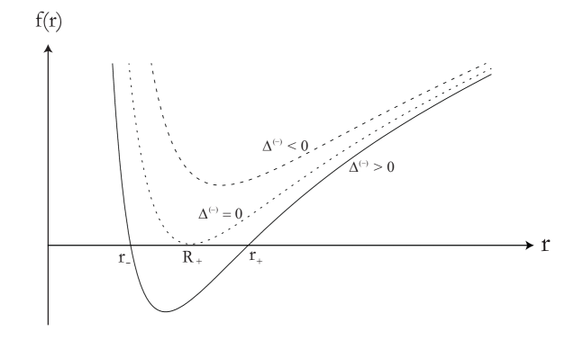
Figure 1: The lapse function for a RNAdS spacetime. Where the upper curve corresponds to a naked singularity, intermediate curve corresponds to an extremal black hole and the lower curve corresponds to a black hole with two horizons.

The Lagrangian for photons in metric (1) is given by

$$2\mathcal{L}=-f(r)\dot{t}^{2}+\frac{\dot{r}^{2}}{f(r)}+r^{2}(\dot{\theta}^{2}+\sin^{2}\theta\dot{\phi}^{2})\equiv 0,$$ (7)

where dot notes derivative respect to proper time $\tau$. The equations of motion can be obtained from

$$\dot{\Pi}_{q}-\frac{\partial\mathcal{L}}{\partial q}=0,$$ (8)

where $\Pi_{q}=\partial\mathcal{L}/\partial\dot{q}$ are the conjugate momenta to coordinate $q$. Since the Lagrangian is independent of ($t,\phi$) the corresponding conjugate momenta are conserved, therefore

$$\Pi_{t}=-f(r)\dot{t}=-\sqrt{E},\qquad\textrm{and}\qquad\Pi_{\phi}=r^{2}\sin^{2}\theta\dot{\phi}=L,$$ (9)

where $E$ and $L$ are constant of motion. From the equation of motion for $\theta$, we have

$$\frac{d(r^{2}\dot{\theta})}{d\tau}=r^{2}\sin\theta\cos\theta\dot{\phi}^{2}.$$ (10)

Without lack of generality we consider that the motion is developed in the invariant plane $\theta=\pi/2$, and our starting equation of motion refereed to coordinates $r$ and $\tau$ is

$$\left(\frac{dr}{d\tau}\right)^{2}=E-V(r),$$ (11)

where $V(r)$ corresponds to the effective potential defined by

$$V(r)=f(r)\frac{L^{2}}{r^{2}}=\left(1-\frac{2M}{r}+\frac{Q^{2}}{r^{2}}+\frac{r^{2}}{\ell^{2}}\right)\frac{L^{2}}{r^{2}}.$$ (12)

In order to describe the photon movement we shall use the impact parameter $b\equiv\frac{L}{\sqrt{E}}$, using the fact that $\dot{r}=(L/r^{2})dr/d\phi$ in (11) we obtain,

$$\left(\frac{dr}{d\phi}\right)^{2}=r^{4}\left(\frac{1}{b^{2}}-\frac{1}{\ell^{2}}\right)-r^{2}+2Mr-Q^{2}.$$ (13)

Dynamical description is completed adding the differential radial equation related to coordinate time

$$\left(\frac{dr}{dt}\right)^{2}=f^{2}(r)\left(1-f(r)\frac{b^{2}}{r^{2}}\right).$$ (14)

It is important to note that for photons the contribution of cosmological constant to the effective potential is a constant (12). Then it does not functionally affect description of the motion in a proper system (11). However, it has an influence in the motion through the coordinate time (14). In this way, photons motion is completely described by the Eqs. (11, 13, 14) and Eq. (9). Following sections are devoted to a detailed study of this motions.

II.1 Radial Motion

Radial motion corresponds to a trajectory with null angular momentum, and we can have photons that move away of singularity and other are doomed to fall to the singularity. From Eqs. (11) and (14) we obtain

$$\frac{dr}{d\tau}=\pm\sqrt{E},$$ (15)

and

$$\frac{dr}{dt}=\pm\frac{F(r)}{\ell^{2}r^{2}},$$ (16)

respectively, and the sign $+$ ($-$) corresponds to photons that to go away (to get closer) from $r_{+}$. If we considered that photons are in $r=r_{i}$ when $t=\tau=0$ and then they approach to $r_{+}$, from Eq. (15) we obtain the well known result of Schwarzschild black hole

$$r(\tau)=r_{i}-\sqrt{E}\tau,$$ (17)

then it takes a proper time $\tau_{+}=(r_{i}-r_{+})/E$ to reach the event horizon. In order to integrated (16) we defined $F(r)=(r-r_{+})(r-r_{-})g(r)$, where

$$g(r)=(r-r_{1})(r-r_{2})=r^{2}+2R_{+}r+[\ell^{2}+3R^{2}_{+}+(r_{+}-R_{+})^{2}].$$ (18)

Then we obtain

$$t(r)=\ln\left[\left(\frac{r-r_{+}}{r_{i}-r_{+}}\right)^{\alpha_{1}}\left(\frac{r-r_{-}}{r_{i}-r_{-}}\right)^{\alpha_{2}}\left(\frac{g(r)}{g(r_{i})}\right)^{\alpha_{3}}\right]+\beta_{1}\left[\arctan\left(\frac{r+R_{+}}{\sqrt{\ell^{2}+3R^{2}_{+}-r_{+}r_{-}}}\right)-\arctan\left(\frac{r_{i}+R_{+}}{\sqrt{\ell^{2}+3R^{2}_{+}-r_{+}r_{-}}}\right)\right],$$ (19)

where the constants are given by

$$\alpha_{1}=\frac{\ell^{2}r^{2}_{+}}{(r_{+}-r_{-})g(r_{+})},\quad\alpha_{2}=-\frac{\ell^{2}r^{2}_{-}}{(r_{+}-r_{-})g(r_{-})},\quad\alpha_{3}=-\frac{\ell^{2}+4R^{2}_{+}}{g(r_{+})g(r_{-})}\ell^{2}R_{+},$$

and

$$\beta_{1}=\frac{[\ell^{2}+3R^{2}_{+}+(r_{+}-R_{+})^{2}][\ell^{2}+6R^{2}_{+}-2r_{+}r_{-}]+2R^{2}_{+}r_{+}r_{-}}{g(r_{+})g(r_{-})[\ell^{2}+3R^{2}_{+}-r_{+}r_{-}]^{1/2}}\ell^{2}.$$

These solutions represents, as in the Schwarzschild case, that photons, in the proper time framework, can cross the event horizon in a finite time and takes and infinity coordinate time. (see Fig. 2)

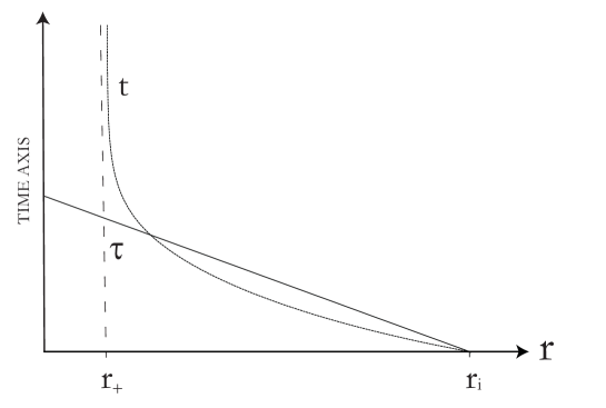
Figure 2: Radial motion of the test particle for the proper time, $\tau$ (solid curve), and the coordinate time, $t$ (dashed curve). Like the Schwarzschild’s solution, photons cross the event horizon in a finite proper time and approaches asymptotically to this in terms of the coordinate time.

II.2 Angular Motion of photons

First, we present brief qualitative description of the allowed angular motions for photons en the RNAdS spacetime.

• Capture Zone: If $0<b\equiv b_{f}<b_{c}$, photons arrive from infinite and then fall to event horizon.

• Critical Trajectories. If $b=b_{c}$, photons can be stayed in one of the unstable inner circular orbit of radius $r_{c}$. Orbit radius is independent of $L$; value of angular momentum $L$ only affects the energy $E_{c}$. Then photons that arrive from infinity can asymptotically fall to a circle of radius $r_{c}$.

• Deflection Zone. If $b_{c}<b=b_{D}<b_{h}$, photons fall from infinite to a minimal distance $r=r_{D}$ and then they can back to infinite. This photons are deflected. The other allowed trajectories correspond to photons moving at the other side of potential barrier, this photons are doomed to fall into the event horizon.

• Pascal Limaçon. For $b=b_{h}$ trajectory of photons are represented by the Pascal Limaçon. This kind of trajectory does not appears in the Schwarzschild or Reissner-Nordstr$\ddot{o}$m cases, then are characteristics trajectories of RNAdS spacetime.

• Confinement Zone. If $b_{h}<b=b_{z}<\infty$, photons fall into the event horizon from an initial distance $r_{0}$.

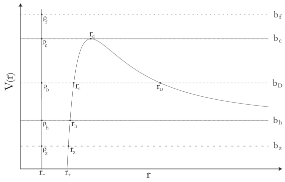
Figure 3: Effective potential for null geodesics in the RNAdS spacetime. Different allowed orbits are characterized by the impact parameter $b$.

In order to do a quantitative analysis, we define the anomalous impact parameter

$$\frac{1}{b^{2}}-\frac{1}{\ell^{2}}=\left\{\begin{array}[]{cl}\frac{1}{B^{2}},\qquad\textrm{if}\quad b<b_{h},\\ \newline \\ -\frac{1}{B_{z}^{2}},\qquad\textrm{if}\quad b=b_{z}>b_{h},\end{array}\right.$$ (20)

then eq. (13) can be rewritten as

$$\left(\frac{dr}{d\phi}\right)^{2}=\frac{r^{4}-B^{2}(r^{2}-2Mr+Q^{2})}{B^{2}}\equiv\frac{P(r)}{B^{2}}.$$ (21)

II.2.1 Captured Photons

The capture zone is defined by values of impact parameter $B=B_{f}$, where radial coordinate $r$ is restricted to values $\rho_{f}\leq r<\infty$ (see Fig. 3). Therefore, characteristic polynomial has two reals roots, $\rho_{f}$ and $\sigma_{f}$ $(\rho_{f}>0>\sigma_{f})$, and two complex roots, $r_{f}$ and $R_{f}$ ($R_{f}=r_{f}^{*}$), and is defined by

$$P_{f}(r)=(r-\rho_{f})(r-\sigma_{f})(r-r_{f})(r-r_{f}^{*}).$$ (22)

Using the change of variables $u=r-\rho_{f}$, and writing the integration in the growing direction of $r$,

$$\phi(u)=B_{f}\int^{u}_{0}\frac{du}{\sqrt{uQ_{f}(u)}},$$ (23)

where the third degree polynomial $Q_{f}(u)$ is given by

$$Q_{f}(u)=(u+u_{1})(u+u_{2})(u+u_{2}^{*}),$$ (24)

and his constants are given by $u_{1}=\rho_{f}-\sigma_{f}$ y $u_{2}=\rho_{f}-r_{f}$. Now using the following constants $\alpha_{f}=(u_{1})^{-1}+(u_{2})^{-1}+(u_{2}^{*})^{-1}$, $\beta_{f}=(u_{1}u_{2})^{-1}+(u_{1}u_{2}^{*})^{-1}+|u_{2}|^{-2}$, $\gamma_{f}=1/C_{f}^{2}$, $\kappa_{f}=\frac{C_{f}}{B_{f}}$ y $C_{f}=|u_{2}|\sqrt{u_{1}}$, and doing the change of variable $u^{-1}=4U-\alpha_{f}/3$, we obtain the quadrature form

$$\kappa_{f}\phi=\int^{\infty}_{U}\frac{dU}{\sqrt{4U^{3}-g_{2_{f}}U-g_{3_{f}}}},$$ (25)

where the invariants are given by,

$$g_{2_{f}}=\frac{1}{4}\left(\frac{\alpha_{f}^{2}}{3}-\beta_{f}\right),\quad\textrm{y}\quad g_{3_{f}}=\frac{1}{16}\left(-\gamma_{f}-\frac{2\alpha_{f}^{3}}{27}+\frac{\alpha_{f}\beta_{f}}{3}\right).$$ (26)

We found the solution of (25) in terms of the elliptic function of Weierstrass, $U=\wp(\kappa_{f}\phi)$, and we can perform the inversion and found the relation between radial and polar coordinates $r$ and $\phi$ (see Fig. 4),

$$r(\phi)=\rho_{f}+\frac{1}{4\wp(\kappa_{f}\phi)-\frac{\alpha_{f}}{3}}.$$ (27)

This equation represents the orbits of captured photons.

Figure 4: Photons which cross both horizons and are reflected at the potential barrier and emerges in another universe.

II.2.2 Critical Orbits of Photons

This critical orbit is a consequence of the potential has a maximum in $r_{c}$ (see Fig: 3), and the photons have a impact parameter $B=B_{c}$. This critical distance can be obtained by the equation $\left(\frac{dV(r)}{dr}\right)_{r=r_{c}}=0$, and yields

$$r_{c}=\frac{3M}{2}\left[1+\sqrt{1-\frac{8Q^{2}}{9M^{2}}}\right].$$ (28)

The unstable circular orbit for photons is independent of the cosmological constant and only depends of the mass and charge of the black hole. In this form, the characteristic polynomial has his general form,

$$P_{c}(r)=(r-\rho_{c})(r-\sigma_{c})|r-r_{c}|^{2}.$$ (29)

We can also obtain the value of $B_{c}$

$$\frac{1}{B_{c}^{2}}=\frac{1}{r_{c}^{2}}\left(1-\frac{2M}{r_{c}}+\frac{Q^{2}}{r_{c}^{2}}\right).$$ (30)

Critical Motion of First Kind

The first kind of critical trajectories corresponds to the motion of photons that came from infinite and reach asymptotically to unstable circular orbit,$r_{c}<r$. In this way, the characteristic polynomial for first kind trajectories, (29), is given by

$$P_{c}(r)=(r-\rho_{c})(r-\sigma_{c})(r-r_{c})^{2}.$$ (31)

Using the change of variables $y=r-r_{c}$ in Eq. (21) we obtain

$$\phi(y)=B_{c}\int^{y}_{\infty}\frac{-dy}{y\sqrt{Q_{c}(y)}},$$ (32)

where second degree polynomial is given by $Q_{c}(y)=(y+y_{1})(y+y_{2})$, whose constant are defined as $y_{1}=r_{c}-\rho_{c}$ and $y_{2}=r_{c}-\sigma_{c}$. Finally using the change $Y=1/y$, and defining $\alpha_{c}=(y_{1})^{-1}+(y_{2})^{-1}$, $\beta_{c}=(y_{1}y_{2})^{-1}$, $\kappa_{c}=\frac{C_{c}}{B_{c}}$ and $C_{c}=\sqrt{y_{1}y_{2}}$, we obtain

$$\kappa_{c}\phi(Y)=\int^{Y}_{0}\frac{dY}{\sqrt{Y^{2}+\alpha_{c}Y+\beta_{c}}},$$ (33)

and

$$\kappa_{c}\phi=\ln\left(a_{{}_{1}}\sqrt{Y^{2}+\alpha_{c}Y+\beta_{c}}+a_{{}_{1}}Y+a_{{}_{2}}\right),$$ (34)

where $a_{{}_{1}}=2(2\sqrt{\beta_{c}}+\alpha_{c})^{-1}$ and $a_{{}_{2}}=\alpha_{c}(2\sqrt{\beta_{c}}+\alpha_{c})^{-1}$. Finally the inversion of (34) allows to find the polar form of the motion

$$r(\phi)=r_{c}+\frac{A_{1}+A_{2}(e^{\kappa_{c}\phi}-a_{{}_{2}})}{A_{3}(e^{\kappa_{c}\phi}-a_{{}_{2}})^{2}-1},$$ (35)

where the constants are given by $A_{1}=\frac{\alpha_{c}}{\beta_{c}}$, $A_{2}=\frac{2}{a_{{}_{1}}\beta_{c}}$ and $A_{3}=\frac{1}{a_{{}_{1}}^{2}\beta_{c}}$. In Fig. 5 we show the form of this orbit.

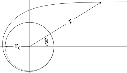
Figure 5: Critical first kind orbit. Photons are coming from the infinity and approach asymptotically to the unstable circular orbit.

Critical motion of second kind

This motion corresponds to photons going to the unstable circular orbit from distance greater than the event horizon but less than critical radius $r_{c}>r>r_{+}$. In this way, the characteristic polynomial given by eq. (29), takes the form

$$P_{c}(r)=(r-\rho_{c})(r-\sigma_{c})(r_{c}-r)^{2}.$$ (36)

Using the change of variables $\widetilde{y}=r_{c}-r$, eq. (21) becomes from (36),

$$\phi(\widetilde{y})=B_{c}\int^{\widetilde{y}}_{\widetilde{y}_{1}}\frac{-d\widetilde{y}}{\widetilde{y}\sqrt{\widetilde{Q}_{c}(\widetilde{y})}},$$ (37)

where $\widetilde{Q}_{c}(\widetilde{y})=(\widetilde{y}_{1}-\widetilde{y})(\widetilde{y}_{2}-\widetilde{y})$, and the constants are the same constants that the first kind motion $\widetilde{y}_{1}=r_{c}-\rho_{c}=y_{1}$, and $\widetilde{y}_{2}=r_{c}-\sigma_{c}=y_{2}$, then $\widetilde{\alpha}_{c}=\alpha_{c}$, $\widetilde{\beta}_{c}=\beta_{c}$, $\widetilde{\kappa}_{c}=\kappa_{c}$, $\widetilde{C}_{c}=C_{c}$, $\widetilde{a}_{{}_{1}}=a_{{}_{1}}$, $\widetilde{a}_{{}_{2}}=a_{{}_{2}}$, $\widetilde{A}_{{}_{1}}=A_{{}_{1}}$ and $\widetilde{A}_{{}_{2}}=A_{{}_{2}}$. Thus we find from eq. (37), and using $\widetilde{Y}=1/\widetilde{y}$, that

$$\kappa_{c}\phi=\ln\left(a_{{}_{1}}\sqrt{Y^{2}-\alpha_{c}Y+\beta_{c}}+a_{{}_{1}}Y-a_{{}_{2}}\right),$$ (38)

and his polar form (see Fig. 6),

$$r(\phi)=r_{c}+\frac{A_{1}-A_{2}(e^{\kappa_{c}\phi}+a_{{}_{2}})}{A_{3}(e^{\kappa_{c}\phi}+a_{{}_{2}})^{2}-1}.$$ (39)

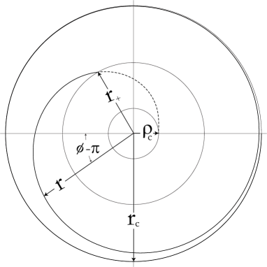
Figure 6: Critical trajectory of second kind. Photons are coming from distances lower than the critical radius and approach asymptotically to the critical radius.

Circular orbits

Once photons travel from infinite, or from another distance $r_{i}$ ($r_{c}>r_{i}>r_{+}$), they go asymptotically to the unstable circular orbit. Their period is practically a constant. Then we can compute this period to respect the proper time,

$$T_{\tau}=\frac{2\pi r_{c}^{2}}{L}=\frac{9\pi M^{2}}{2L}\left[1+\sqrt{1-\frac{8Q^{2}}{9M^{2}}}\right]^{2},$$ (40)

while the period in coordinate time is

$$T_{t}=\frac{2\pi r_{c}^{2}}{L}\frac{\sqrt{E_{c}}}{f(r_{c})}=T_{\tau}\frac{\sqrt{E_{c}}}{f(r_{c})}=\frac{2\pi r_{c}}{\sqrt{f(r_{c})}}.$$ (41)

The above results show that both periods do not depend of the cosmological constant.

Schwarzschild Limit

Considering the circular movement of photons, the unstable radius is $3M$, then periods to circular orbits for photons reduce to the following terms $T_{\tau}=\frac{18\pi M^{2}}{L}$ and $T_{t}=6\pi M\sqrt{3}$ Shutz .

II.2.3 Deflection Zone

In this case, we have that anomalous impact parameter is $B_{{}_{D}}$, and from Fig. 3, there are two possibilities for photons with this impact parameter. In the trajectory of first class the photons came from infinite and are deflected, approaching to a minimal distance in $r=r_{{}_{D}}$ and going away to infinite ($r_{+}<r_{a}<r_{{}_{D}}<r$); in the trajectory of second class the photon motion is allowed between two distance $r_{+}<r<r_{a}<r_{{}_{D}}$. The extremal distances $r_{{}_{D}}$ and $r_{a}$ are obtained from the extremal condition $\frac{dr}{d\phi}\mid_{r_{extr}}=0$. On the other side, the polynomial of fourth degree has four real roots, and it can be written in a general form

$$P_{{}_{D}}(r)=|r-r_{{}_{D}}|\,|r-r_{a}|\,(r-\rho_{{}_{D}})\,(r-\sigma_{{}_{D}}).$$ (42)

First class trajectory:

This trajectory corresponds to the light deflection. We start computing the trajectory from the extremal point $r_{{}_{D}}$ and using the change of variable $w=r-r_{D}$, we obtain

$$\phi(w)=B_{{}_{D}}\int^{w}_{0}\frac{dw}{\sqrt{wQ_{{}_{D}}(w)}},$$ (43)

where third degree polynomial in the new variable is $Q_{{}_{D}}(w)=(w_{1}+w)(w_{2}+w)(w_{3}+w)$, where $w_{1}=r_{{}_{D}}-r_{a}$, $w_{2}=r_{{}_{D}}-\rho_{{}_{D}}$ and $w_{3}=r_{{}_{D}}-\sigma_{{}_{D}}$. Now defining the constants $\alpha_{{}_{D}}=(w_{1})^{-1}+(w_{2})^{-1}+(w_{3})^{-1}$, $\beta_{{}_{D}}=(w_{1}w_{2})^{-1}+(w_{1}w_{3})^{-1}+(w_{2}w_{3})^{-1}$, $\gamma_{{}_{D}}=C_{{}_{D}}^{-2}$, $\kappa_{{}_{D}}=\frac{C_{{}_{D}}}{B_{{}_{D}}}$, $C_{{}_{D}}=\sqrt{w_{1}w_{2}w_{3}}$, and doing the change of variable $w^{-1}=4W-\alpha_{{}_{D}}/3$, Eq. (43) give us

$$\kappa_{{}_{D}}\phi=\int^{\infty}_{W}\frac{dW}{\sqrt{4W^{3}-g_{2_{D}}W-g_{3_{D}}}},$$ (44)

where the invariants are

$$g_{2_{D}}=\frac{1}{4}\left(\frac{\alpha_{{}_{D}}^{2}}{3}-\beta_{{}_{D}}\right),\qquad\textrm{y}\qquad g_{3_{D}}=\frac{1}{16}\left(\frac{\alpha_{{}_{D}}\beta_{{}_{D}}}{3}-\gamma_{{}_{D}}-\frac{2\alpha_{{}_{D}}^{3}}{27}\right),$$ (45)

whose solution is $W=\wp(\kappa_{{}_{D}}\phi)$. This gives the parametric relation (see Fig. 7)

$$r(\phi)=r_{{}_{D}}+\frac{1}{4\wp(\kappa_{{}_{D}}\phi)-\frac{\alpha_{{}_{D}}}{3}},$$ (46)

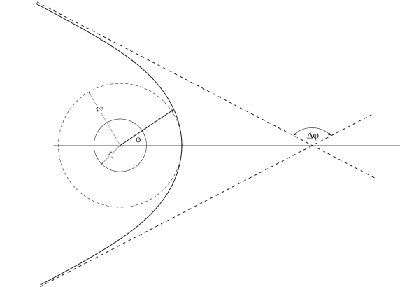
Figure 7: Light deflection in the background of a RNAdS black hole. The figure shows the deflection angle $\Delta\varphi$.

The angle of deflection for photons is defined by

$$\Delta\varphi=2|\phi(\infty)-\phi(r_{{}_{D}})|-\pi,$$ (47)

or in terms of the inverse Weierstrass function

$$\Delta\varphi=\frac{2}{\kappa_{{}_{D}}}\wp^{-1}\left(\frac{\alpha_{{}_{D}}}{12}\right)-\pi.$$ (48)

Second class trajectories:

In this case photons have a maximal distance of remoteness, $r_{a}$. This distance can be chosen as the starting point of trajectory. Using the change of variable $x=r_{a}-r$, we can obtain

$$\phi(x)=B_{{}_{D}}\int^{x}_{0}\frac{dx}{\sqrt{x\widetilde{Q}_{{}_{D}}(x)}},$$ (49)

where the cubic polynomial is given by $\widetilde{Q}_{D}(x)=(x+x_{1})(x_{2}-x)(x_{3}-x)$, and the corresponding constants are given by $x_{1}=r_{{}_{D}}-r_{a}$, $x_{2}=r_{a}-\rho_{{}_{D}}$ y $x_{3}=r_{a}-\sigma_{{}_{D}}$. Beside, we use the following definition $\widetilde{\alpha}_{{}_{D}}=-(x_{1})^{-1}+(x_{2})^{-1}+(x_{3})^{-1}$, $\widetilde{\beta}_{{}_{D}}=(x_{1}x_{2})^{-1}+(x_{1}x_{3})^{-1}-(x_{2}x_{3})^{-1}$, $\widetilde{\gamma}_{{}_{D}}=\widetilde{C}_{{}_{D}}^{-2}$, $\widetilde{\kappa}_{{}_{D}}=\frac{\widetilde{C}_{{}_{D}}}{B_{{}_{D}}}$ $\widetilde{C}_{{}_{D}}=\sqrt{x_{1}x_{2}x_{3}}$, and doing the following change of variable $x=4X+\alpha_{D}/3$ in Eq. (21), we obtain

$$\widetilde{\kappa}_{{}_{D}}\phi=\int^{\infty}_{X}\frac{dX}{\sqrt{4X^{3}-\widetilde{g}_{2_{D}}X-\widetilde{g}_{3_{D}}}},$$ (50)

whose solution is $X=\wp(\widetilde{\kappa}_{{}_{D}}\phi)$, where the invariant are given by

$$\widetilde{g}_{2_{D}}=\frac{1}{4}\left(\frac{\alpha_{{}_{D}}^{2}}{3}+\beta_{{}_{D}}\right),\qquad\textrm{y}\qquad\widetilde{g}_{3_{D}}=\frac{1}{16}\left(\frac{\alpha_{{}_{D}}\beta_{{}_{D}}}{3}-\gamma_{{}_{D}}+\frac{2\alpha_{{}_{D}}^{3}}{27}\right).$$ (51)

Inverting to obtain the coordinate $r$ as a function of $phi$, we obtain the polar equation for the orbits

$$r(\phi)=r_{a}-\frac{1}{4\wp(\widetilde{\kappa}_{{}_{D}}\phi)+\frac{\widetilde{\alpha}_{{}_{D}}}{3}}.$$ (52)

The above solution is shown in Fig. 8.

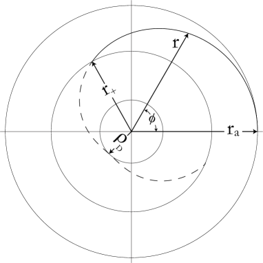
Figure 8: Many-world bound orbit for null geodesics of second class.

II.2.4 Pascal Limaçon

This kind of trajectory is an unique solution for the geodesic problem of RNAdS. It corresponds to one epicycle curve defined by his anomalous impact parameter $B_{h}\rightarrow\infty$ ($b_{h}=\ell$). Therefore, radial coordinate is restricted to $r_{+}<r<r_{h}$, and the equation of motion (21) can be written as

$$\phi(r)=\int_{r_{h}}^{r}\frac{-dr}{\sqrt{Q_{h}(r)}},$$ (53)

where the second degree polynomial is defined by $Q_{h}(r)=(r_{h}-r)(r-\rho_{h})$, and his roots are: $r_{h}=M+\sqrt{M^{2}-Q^{2}}$ y $\rho_{h}=M-\sqrt{M^{2}-Q^{2}}$. It is straightforward to find solution of Eq. (53) (see Fig. 9), which is given by

$$r(\phi)=M+\sqrt{M^{2}-Q^{2}}\cos\phi.$$ (54)

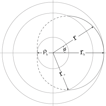
Figure 9: Many-world bound orbit for null geodesics, which is described by a Pascal Limaçon. If $Q=0$, the trajectory is a cardioid.

Note that this trajectory is an exclusive solution of black hole with cosmological constant and it does not depend on its value

II.2.5 Confined Photons

In this case, photons have an anomalous impact parameter $B_{z}$, con $b_{z}>b_{h}$. In this region radial coordinate is restricted to $r_{+}<r<r_{z}$, and the characteristic polynomial has two different real roots, $\rho_{z}$ y $r_{z}$ ($\rho_{z}<r_{z}$), beside to a conjugate pair $r_{2}$ y $R_{2}$ ($R_{2}=r_{2}^{*}$). Using $\phi=0$ for $r=r_{z}$, together which the change of variable $s=r_{z}-r$, we obtain

$$\phi(r)=B_{z}\int^{s}_{s_{z}}\frac{ds}{\sqrt{sQ_{z}(s)}},$$ (55)

where the third degree polynomial in the new variable is $Q_{z}(s)=(s_{1}-s)(s_{2}-s)(s_{2}^{*}-s)$, and the constants are $s_{1}=r_{z}-\rho_{z}$ y $s_{2}=r_{z}-r_{2}$. Using the constants $\alpha_{z}=(s_{1})^{-1}+(s_{2})^{-1}+(s_{2}^{*})^{-1}$, $\beta_{z}=(s_{1}s_{2})^{-1}+(s_{1}s_{2}^{*})^{-1}+|s_{2}|^{-2}$, $\gamma_{z}=C_{z}^{-2}$, $\kappa_{z}=\frac{C_{z}}{B_{z}}$, and $C_{z}=|s_{2}|\sqrt{s_{1}}$, together the change of variable $s^{-1}=4S+\alpha_{z}/3$, we obtain

$$\kappa_{z}\phi(S)=\int^{\infty}_{S}\frac{dS}{\sqrt{4S^{3}-g_{2_{z}}S-g_{3_{z}}}},$$ (56)

where the invariant are

$$g_{2_{z}}=\frac{1}{4}\left(\frac{\alpha_{z}^{2}}{3}-\beta_{z}\right),\quad\textrm{y}\quad g_{3_{z}}=\frac{1}{16}\left(\gamma_{z}+\frac{2\alpha_{z}^{3}}{27}-\frac{\alpha_{z}\beta_{z}}{3}\right).$$ (57)

Again the solution of (56) is obtained in terms of the Weierstrass function $\wp$, $S=\wp(\kappa_{z}\phi)$, where the inversion give us the polar equation of confined orbit (see Fig. 10)

$$r(\phi)=r_{z}-\frac{1}{4\wp(\kappa_{z}\phi)+\frac{\alpha_{z}}{3}}.$$ (58)

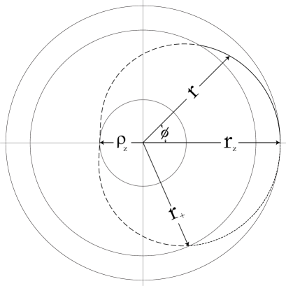
Figure 10: Many-world bound orbit for confined photons

III Final Remarks

We have studied the geodesic structure of RNAdS black holes analyzing the behavior of null geodesic by means of the effective potential which appears in the radial equation of motion. We separated our study in two cases, radial null geodesics and angular null geodesics. We have obtained, for the radial case, analytical solutions for the proper and coordinate time. Our solutions are very similar to Schwarzschild case where in the proper time framework photons can cross the event horizon and in a finite but is infinity in the coordinate time framework. In the angular motions of photons we have found that are different kind of motions depending of the impact parameter (b) of the orbits. We have obtained five different kinds of motions for captured photons, which arrive from infinite and fall into the event horizon. The trajectories of these null geodesics have been given in terms of elliptic function of Weierstrass. In second place, we have also found photons following critical orbits, representing movements that came from infinite and can asymptotically to fall to a circle. Third, we have found the deflection zone that represents photons falling from infinite to a minimal distance and then going back to infinite again. The fourth kind of orbit is described by Pascal Limaçon. This trajectory is an exclusive solution of black hole which cosmological constant and has the particularity that does not depend of the value of cosmological constant. Finally, our last kind of orbit represents confined photons moving in the region $r_{+}<r<r_{z}$.

- (1) A. Einstein, Preuss. Akad. Wiss. Berlin Sitzber., 1917, 142.
- (2) A. G. Riess et al. [ Supernova Search Team Collaboration ], Astrophys. J. 607, 665-687 (2004).
- (3) P. J. E. Peebles, B. Ratra, Rev. Mod. Phys. 75, 559-606 (2003).
- (4) E. J. Copeland, M. Sami, S. Tsujikawa, Int. J. Mod. Phys. D15, 1753-1936 (2006). [hep-th/0603057].
- (5) P. J. E. Peebles, 1998, astro-ph/9806201.
- (6) V. F. Shvartsman, Sov. Phys. JETP 33, 475 (1970).
- (7) B. Punsly, Black Hole Gravitohydromagnetics, Springer, (2001).
- (8) L. Neslusan, AA 372, 913 (2001).
- (9) T. Damour, R. Ruffini, Phys. Rev. Lett. 35, 463 (1975).
- (10) C. Cherubini, A. Geralico, J. Rueda, and R. Ruffini, Phys.Rev.D79:124002, (2009); Remo Ruffini, Gregory Vereshchagin, She-Sheng Xue, Physics Reports, Volume 487, Issue 1-4, p. 1-140 (2010)
- (11) F. Kottler, Annalen Physik 56, 410 (1918).
- (12) M. J. Jaklitsch, C. Hellaby and D. R. Matravers, Gen. Rel. Grav. 21 (1989) 941.
- (13) Z. Stuchlík and M. Calvani, Gen. Rel. Grav., 23, 507 (1991).
- (14) G. V. Kraniotis and S. B. Whitehouse, Class. Quantum Grav., 20, 4817-4835 (2003).
- (15) G. V. Kraniotis, Class. Quantum Grav., 21, 4743-4769 (2004).
- (16) Z. Stuchlík and S. Hledík, Phys. Rev. D, 60, 044006 (1999).
- (17) N. Cruz, M. Olivares and J. R. Villanueva Class. Quantum Grav., 22, 1167-1190 (2005).
- (18) Z. Stuchlík and S. Hledík, Acta Phys. Slov., 52, 363 (2002).
- (19) E. Hackmann, V. Kagramanova, J. Kunz and C. Lammerzahl, Phys. Rev. D 78, 124018 (2008) [Erratum-ibid. 79, 029901 (2009)]
- (20) E. Hackmann and C. Lammerzahl, Phys. Rev. D 78, 024035 (2008).
- (21) E. Hackmann and C. Lammerzahl, Phys. Rev. Lett. 100, 171101 (2008).
- (22) Z. Stuchlík and P. Slany, Phys. Rev. D, 69, 064001 (2004).
- (23) D. Pugliese, H. Quevedo and R. Ruffini, arXiv:1105.2959 [gr-qc].
- (24) D. Pugliese, H. Quevedo and R. Ruffini, arXiv:1003.2687 [gr-qc].
- (25) D. Pugliese, H. Quevedo and R. Ruffini, Phys. Rev. D 83, 104052 (2011) [arXiv:1103.1807 [gr-qc]].
- (26) M. Olivares, J. Saavedra, C. Leiva and J. R. Villanueva, arXiv:1101.0748 [gr-qc].
- (27) B. Shutz, A first course in general relativity, Cambridge university press, (1990).