Galaxy Zoo: The Environmental Dependence of Bars and Bulges in Disc Galaxies

Abstract

We present an analysis of the environmental dependence of bars and bulges in disc galaxies, using a volume-limited catalogue of 15810 galaxies at $z<0.06$ from the Sloan Digital Sky Survey with visual morphologies from the Galaxy Zoo 2 project. We find that the likelihood of having a bar, or bulge, in disc galaxies increases when the galaxies have redder (optical) colours and larger stellar masses, and observe a transition in the bar and bulge likelihoods at $M_{\ast}=2\times 10^{10}\,M_{\odot}$, such that massive disc galaxies are more likely to host bars and bulges. In addition, while some barred and most bulge-dominated galaxies are on the “red sequence” of the colour-magnitude diagram, we see a wider variety of colours for galaxies that host bars. We use galaxy clustering methods to demonstrate statistically significant environmental correlations of barred, and bulge-dominated, galaxies, from projected separations of $150\,\mathrm{kpc}/h$ to $3\,\mathrm{Mpc}/h$. These environmental correlations appear to be independent of each other: i.e., bulge-dominated disc galaxies exhibit a significant bar-environment correlation, and barred disc galaxies show a bulge-environment correlation. As a result of sparse sampling tests—our sample is nearly twenty times larger than those used previously—we argue that previous studies that did not detect a bar-environment correlation were likely inhibited by small number statistics. We demonstrate that approximately half of the bar-environment correlation can be explained by the fact that more massive dark matter haloes host redder disc galaxies, which are then more likely to have bars; this fraction is estimated to be $50\pm 10~{}\%$ from a mock catalogue analysis and $60\pm 5~{}\%$ from the data. Likewise, we show that the environmental dependence of stellar mass can only explain a smaller fraction ($25\pm 10~{}\%$) of the bar-environment correlation. Therefore, a significant fraction of our observed environmental dependence of barred galaxies is not due to colour or stellar mass dependences, and hence must be due to another galaxy property, such as gas content, or to environmental influences. Finally, by analyzing the projected clustering of barred and unbarred disc galaxies with halo occupation models, we argue that barred galaxies are in slightly higher-mass haloes than unbarred ones, and some of them (approximately 25%) are satellite galaxies in groups. We discuss the implications of our results on the effects of minor mergers and interactions on bar formation in disc galaxies.

1 Introduction

In recent years, there has been a resurgence in interest in the “secular” processes that could affect galaxy evolution (e.g., Weinzirl et al. 2009; Schawinski et al. 2010; Emsellem et al. 2011), driven by the growing understanding that major mergers are rare (e.g., Hopkins et al. 2010b; Darg et al. 2010; Lotz et al. 2011), and may not play as important a role in galaxy evolution as had previously been thought (Parry et al. 2009; Davé et al. 2011). In particular, bars have been found to be common structures in disc galaxies, and are thought to affect the evolution of galaxies (e.g., Sellwood & Wilkinson 1993; Kormendy & Kennicutt 2004) and the dark matter haloes that host them (e.g., Debattista & Sellwood 2000; Weinberg & Katz 2002). The abundance and properties of barred galaxies have been analyzed in low and high-redshift surveys (e.g., Jogee et al. 2005; Sheth et al. 2005, 2008; Barazza et al. 2008; Aguerri et al. 2009; Nair & Abraham 2010; Cameron et al. 2010; Masters et al. 2011; Hoyle et al. 2011; Ellison et al. 2011) and have been modeled with detailed numerical simulations, including their interactions with the host dark matter haloes (e.g., Valenzuela & Klypin 2003; O’Neill & Dubinski 2003; Debattista et al. 2006; Heller et al. 2007; Weinberg & Katz 2007).

Bars are extended linear structures in the central regions of galaxies, which form from disc instabilities and angular momentum redistribution within the disc (e.g., Athanassoula 2003; Berentzen et al. 2007; Foyle et al. 2008). Bars are efficient at driving gas inwards, perhaps sparking central star formation (e.g., Friedli et al. 1994; Ellison et al. 2011), and thus may help to grow a central bulge component in galaxy discs (e.g., Dalcanton et al. 2004; Debattista et al. 2006; Gadotti 2011). Such bulges are sometimes referred to as “pseudo-bulges”, to distinguish them from “classical” bulges, which are often thought to have formed from the hierarchical merging of smaller objects (e.g., Kormendy & Kennicutt 2004; Drory & Fisher 2007; De Lucia et al. 2011; Fontanot et al. 2011).

Bars and (classical) bulges may also be related structures and in some cases could form simultaneously. Galaxies with earlier-type morphologies, which have more prominent bulges, tend to have more, and longer, bars (Elmegreen & Elmegreen 1985; Weinzirl et al. 2009; Masters et al. 2011; Hoyle et al. 2011; Elmegreen et al. 2011; cf., Barazza et al. 2008). In addition, at least in some galaxies, the bars and bulges have similar stellar populations (Sánchez-Blázquez et al. 2011). Nonetheless, there are some barred galaxies that lack bulges and many bulge-dominated galaxies that lack bars (e.g., Laurikainen et al. 2007; Pérez & Sánchez-Blázquez 2011).

Various classification methods have been developed to observationally identify bars, either visually or using automated techniques, such as ellipse-fitting of isophotes and Fourier decomposition of surface brightness distributions (e.g., Erwin 2005; Aguerri et al. 2009; Gadotti 2009). These have yielded similar, but not always consistent, bar fractions (see discussions in Sheth et al. 2008; Nair & Abraham 2010; Masters et al. 2011). All bar identification methods are affected by issues such as inclination, spatial resolution, wavelength dependence, surface brightness limits, and selection biases (e.g., Menéndez-Delmestre et al. 2007).

In this paper, we use data from the Galaxy Zoo 2 project (see Masters et al. 2011), which provides detailed visual classifications of $\sim 250,000$ galaxies in the Sloan Digital Sky Survey (SDSS; York et al. 2000). Galaxy Zoo yields a relatively large catalogue of galaxies with reliable classifications in a variety of environments. It is particularly suited for analyses of the environmental dependence of the morphological and structural properties of galaxies across a range of scales, as the large volume and sample size makes it less affected by cosmic variance than other catalogues.

It has long been known that galaxy morphologies are correlated with the environment, such that spiral galaxies tend to be located in low-density regions and early-type galaxies in denser regions (e.g., Dressler 1980; Postman & Geller 1984; and confirmed by Galaxy Zoo: Bamford et al. 2009; Skibba et al. 2009). There are a variety of ways to assess the correlation between galaxy properties and the environment, such as fixed aperture counts and distances to nearest neighbors (see reviews by Haas et al. 2012; Muldrew et al. 2012). We follow Skibba & Sheth (2009) and Skibba et al. (2009) by using two-point galaxy clustering.

There has been some recent work focused specifically on the environmental dependence of barred galaxies (van den Bergh 2002; Li et al. 2009; Aguerri et al. 2009; Méndez-Abreu et al. 2010; Giordano et al. 2011). All of these studies argue that there is little to no dependence of galaxy bars on the environment. Contrary to these results, Barazza et al. (2009) and Marinova et al. (2009, 2012) detect a slightly larger bar fraction in the cores of galaxy clusters, but of weak statistical significance, and Barway et al. (2011) find a higher bar fraction of faint S0s in group/cluster environments. There is as yet no consensus on the environmental dependence of galaxy bars. These studies have been hampered by small number statistics, having typically a few hundred to a thousand galaxies at most. We improve upon this work by analyzing the environmental dependence galaxy bars and bulges in Galaxy Zoo 2, using a volume-limited catalogue consisting of 15810 disc galaxies in the SDSS.

This paper is organized as follows. In the next section, we describe the Galaxy Zoo 2 data and our volume-limited catalogue. We introduce mark clustering statistics, and in particular, the marked correlation function, in Section 3. In Section 4, we show the distributions and correlations between measures of bars and bulges. Then in Section 5, we present some of our main results, about the environmental dependence of barred and bulge-dominated galaxies, and we interpret the results with mock catalogues and halo occupation models in Section 6. We end with a discussion of our results in Section 7.

2 Data

2.1 Morphological Information from Galaxy Zoo

To identify bars in local galaxies we use classifications provided by members of the public through the Galaxy Zoo website. Specifically, we use classifications from the second phase of Galaxy Zoo (hereafter GZ2) which ran for 14 months (between 9th Feb 2009 and 22nd April 2010). In GZ2, volunteers were asked to provide detailed classifications for the brightest (in terms of flux) 250,000 galaxies in the SDSS Data Release 7 (DR7; Abazajian et al. 2009) Main Galaxy Sample (MGS; Strauss et al. 2002). The selection criteria for GZ2 are $m_{r}<17$ and $r_{90}>3$″, where $m_{r}$ is the $r$-band Petrosian magnitude, and $r_{90}$ is the radius containing 90% of this flux. Additionally, where the galaxy has a measured redshift, the selection $0.0005<z<0.25$ is applied.

Following the method of the original Galaxy Zoo (Lintott et al. 2008, 2011; hereafter GZ1), volunteers were asked to classify galaxies from the $gri$ composite images. The complete GZ2 decision tree is shown in Fig. 1 of Masters et al. (2011). Users were presented each question in turn, with their progress down the tree depending on their previous answers. In the 14 months GZ2 ran, 60 million individual classifications were collected, with each galaxy in GZ2 having been classified by a median of 40 volunteers (i.e., 40 people answering the question at the top of the tree). As was discussed for GZ1 in Lintott et al. (2008) and Bamford et al. (2009), the conversion of these raw clicks into a unique classification for each galaxy is a process similar to data reduction that must take into account possible spurious classifications and other problems. An iterative weighting scheme is used to remove the influence of unreliable users, and a cleaning procedure is applied to remove multiple classifications of the same galaxy by the same user.

In what follows we will call the total number of cleaned and weighted classifications for a given question, $N_{X}$, and the fraction of positive answers to a given question $p_{X}$. For example, we will discuss $N_{\rm total}$, which is the total (weighted) number of users classifying a given galaxy; $p_{\rm features}$, the (weighted) fraction of such users identifying the galaxy as having features; $N_{\rm bar}$, the total (weighted) number of classifications to the “bar question”; and $p_{\rm bar}$, the (weighted) fraction of users who indicated that they saw a bar.

Examples of disc galaxies with a range of $p_{\rm bar}$ are shown in Figure 1. The top row shows four randomly selected galaxies with $p_{\rm bar}=0.0$ (and a range of values of fracdeV, which is used to indicate the bulge size; see Sec. 2.2 for details). The lower rows show galaxies with larger values of $p_{\rm bar}$; the galaxies in the bottom row clearly have strong bars.

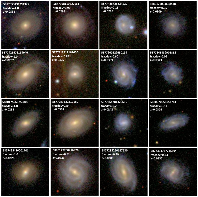
Figure 1: Example images of disc galaxies with a range of values of $p_{\rm bar}$ and fracdeV. The top row shows four randomly selected galaxies with $p_{\rm bar}=0.0$ (and a range of values of fracdeV, as indicated). The second row shows galaxies with $p_{\rm bar}=0.2$, then $p_{\rm bar}=0.5$ in the row below, and finally $p_{\rm bar}=1.0$ in the bottom row.

2.2 Bulge Sizes

While bulge size identification was present in the GZ2 classification scheme (in the question of “How prominent is the central bulge?”), we choose instead to follow Masters et al. (2010a) and use the SDSS parameter “fracdeV”, which is a continuous indicator of bulge sizes in disc galaxies (see Kuehn & Ryden 2005; Bernardi et al. 2010) and is strongly correlated with the GZ2 bulge classification (Masters et al. 2011). In the SDSS pipeline (Subbarao et al. 2002), galaxy light profiles are fit with both an exponential and de Vaucouleurs profile (de Vaucouleurs 1948), and the model magnitude comes from the best fit linear combination of these two profiles. The parameter fracdeV indicates the fraction of this model $r$-band magnitude that is contributed by the de Vaucouleur profile (Vincent & Ryden 2005). It is expected to have the value fracdeV$=1$ in elliptical galaxies, and also bulge-dominated disc galaxies whose central light is dominated by a spheroidal bulge component. In pure disc galaxies with no central light excess over an exponential disc, fracdeV$=0$ is expected. As we will see in Section 4, many galaxies have either fracdeV$=0$ or 1.

The fracdeV parameter is likely to be most effective at identifying classical bulges, although any central excess of light over an exponential disc will drive fracdeV away from a zero value (Masters et al. 2010a). The Sérsic index, which is closely related to fracdeV (Vincent & Ryden 2005), is correlated with the bulge-to-total luminosity ratio, but with some scatter (Gadotti 2009). Gadotti (2009) also shows that the Sérsic index can be used to distinguish between classical and pseudo-bulges, although it cannot perfectly separate them (see also Graham 2011). The concentration $r_{90}/r_{50}$, the ratio of the radii containing 90% and 50% of a galaxy’s light in the $r$-band, is another morphological indicator (Strateva et al. 2001), and we have found that it exhibits a qualitatively similar clustering dependence as fracdeV. A comparison between fracdeV, concentration, and GZ1 spiral and early-type classifications is shown in Masters et al. (2010a).

2.3 Other Galaxy Properties

In addition to morphological classifications and light profile shapes, we use various other parameters from the SDSS, including redshifts, $(g-r)$ and $(g-i)$ colours (from the model magnitudes), $M_{r}$ and $M_{i}$ total magnitudes (for which we use the Petrosian magnitudes), and axial ratio, $\mathrm{log}(a/b)$ (from the exponential model axial ratio fit in the $r$-band). All magnitudes and colours are corrected for Galactic extinction using the maps of Schlegel, Finkbeiner & Davis (1998) and are $K$-corrected to $z=0.0$ using kcorrect v4_2 (Blanton & Roweis 2007).

We compute stellar masses using the Zibetti et al. (2009) stellar mass calibration, which is based on the total magnitude ${{}^{0.0}M_{i}}$ and ${}^{0.0}(g-i)$ colour (the superscript “0.0” refers to the redshift of the $K$-correction), with an absolute solar magnitude of $M_{i,\odot}=4.52$ (Blanton et al. 2001), and assuming a Chabrier initial mass function (Chabrier et al. 2003). We refer the reader to Zibetti et al. (2009) for details of the model.

The stellar mass-to-light ratios typically have $0.2-0.3$ dex scatter. A more accurate method to estimate stellar masses would have been to apply stellar population models (e.g., Maraston 2005) directly to the SDSS photometry in all five optical passbands. The Zibetti et al. (2009) calibration (which uses an updated version of Bruzual & Charlot (2003) models) is nonetheless consistent with Maraston (2005), with no systematic offsets between their masses and with discrepancies only at young stellar ages, and is sufficient for the analysis in this paper.

2.4 Volume-Limited Disc Galaxy Sample

We perform our analysis on a volume-limited sample. Our catalogue is a subsample of the GZ2 catalogue, with limits $-23.5<{{}^{0.0}M_{r}}-5\mathrm{log}(h)\leq-19.4$ and $0.017\leq z<0.060$. This catalogue is similar to the volume-limited catalogue used in Skibba et al. (2009; hereafter S09), but it has a slightly fainter absolute magnitude threshold because it is limited to slightly lower redshifts where we expect the bar identification in GZ2 to be most reliable (see Masters et al. 2011, hereafter M11, and Hoyle et al. 2011 for further discussion of this choice); in addition, GZ2 has a slightly brighter flux limit than GZ1.

The absolute magnitude threshold of our volume-limited catalogue approximately corresponds to $M_{r}<M^{\ast}+1$, where $M^{\ast}$ is the Schechter function break in the $r$-band luminosity function (Blanton et al. 2001). It also corresponds to an approximate stellar mass threshold of $\approx 4\times 10^{9}\,M_{\odot}$ (Zibetti et al. 2009) and a halo mass threshold of $\approx 5\times 10^{11}\,h^{-1}\,M_{\odot}$ (Skibba & Sheth 2009), although there is substantial scatter between galaxy luminosity and stellar and halo masses.

The absolute magnitude and redshift limits result in a catalogue of 45581 galaxies. We limit the sample further to $\mathrm{log}(a/b)<0.3$, which is approximately an inclination of $60^{\circ}$, in order to select face-on or nearly face-on galaxies. This is a comparable inclination cut to other recent studies of bars (e.g., Barazza et al. 2008; Sheth et al. 2008; Aguerri et al. 2009) and identical to the cut used by M11 to study the bar fraction of GZ2. After this inclination cut, the catalogue is reduced to 32019 galaxies.

We require a reasonable number of answers to the bar identification question in GZ2. As can been seen in the GZ2 classification tree, in order to identify the presence of a bar in a galaxy, the volunteer must first identify the galaxy as “having features”, and in addition answer “no” to the question “Could this be an edge-on disc?” We therefore limit the sample to $N_{\rm bar}\geq N_{\rm total}/4$ (which is equivalent to $p_{\rm features}p_{\rm notedge-on}\geq 0.25$), resulting in a catalogue of 15989 galaxies. We also remove a small number (179) of objects with $N_{\rm bar}<10$ which may have bar identifications dominated by a small number of classifiers.

Our resulting volume-limited catalogue comprises 15810 nearly face-on disc galaxies with reliable bar classifications. The galaxy distribution in redshift and magnitude, and the cuts used to define the catalogue, are shown in Figure 2. Note that, because of the $N_{\mathrm{bar}}$ cuts, elliptical galaxies are excluded from the sample. We emphasize that only disc galaxies (i.e., spiral galaxies and S0s) constitute the sample, including “bulge-dominated” disc galaxies and “pure disc” galaxies, to which we often refer as “disc-dominated” galaxies. We will distinguish between bulge-dominated and disc-dominated galaxies with the fracdeV parameter (described in Sec. 2.2).

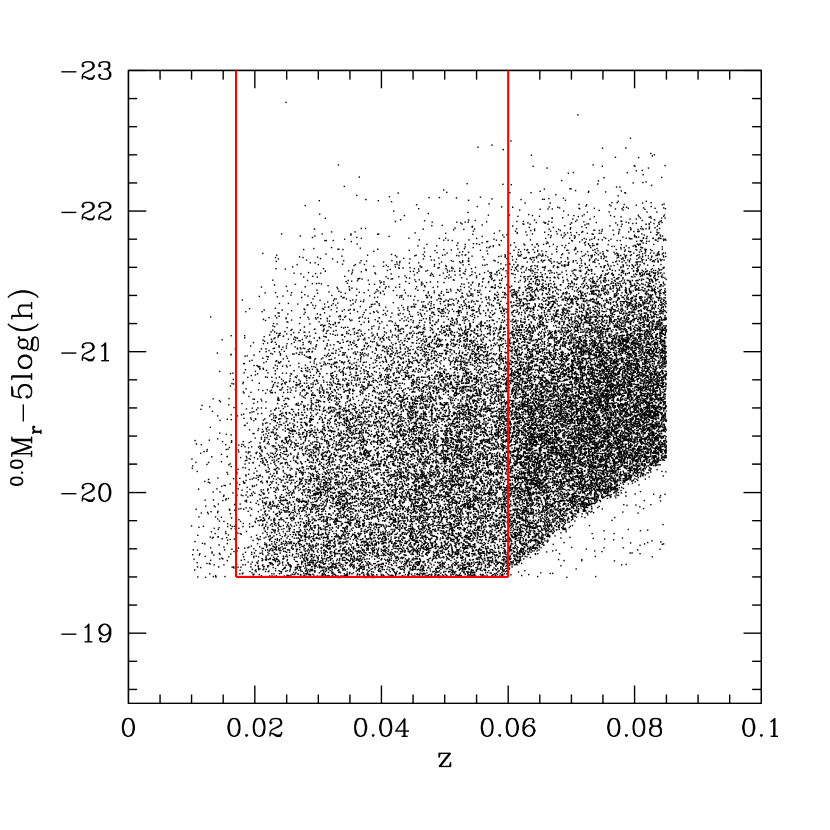
Figure 2: Distribution in redshift and Petrosian $r$-band absolute magnitude, with the selection criteria of the volume-limited catalogue: $-23.5<{{}^{0.0}M_{r}}-5\mathrm{log}(h)\leq-19.4$ and $0.017\leq z<0.060$. Without the $N_{\mathrm{bar}}$ classification cut (selecting galaxies with sufficient classifications) and $a/b$ axis ratio cut (selecting nearly face-on disc galaxies), the magnitude-redshift distribution is virtually identical; these cuts do not bias the catalogue.

In principle, some of the selection criteria, such as the $N_{\mathrm{bar}}$ requirements, could bias our results by excluding certain galaxies in an environmentally dependent way. Nevertheless, M11 have tested this by comparing the luminosity, colour, axial ratio, and redshift distributions with and without this requirement, and have found no significant differences. Therefore, it is unlikely that there are any significant biases introduced; on the contrary, these criteria should eliminate biases by removing contaminating objects, such as elliptical galaxies or mergers with unreliable bar classifications.

We have also tested our clustering measurements as a function of the axial ratio $a/b$, and confirmed that they are not affected by the inclination cut. In particular, the correlation functions for different inclinations are within 0.03 dex ($7\%$), well within the error bars, and the mark correlation functions, described in the next section, are within $2\%$, except at separations of $r_{p}<500~{}\mathrm{kpc}/h$, where they still agree within $10\%$.

In addition, “fiber-collided” galaxies are not included in the catalogue. The thickness of the spectroscopic fibers means that some galaxies closer than $55\arcsec$ on the sky will be missing spectra and redshifts. This fiber-collision constraint is partly alleviated by the fact that neighbouring plates have overlap regions, but it still results in $7\%$ of targeted galaxies not having a measured redshift (Zehavi et al. 2005) and could significantly affect clustering measurements, especially at separations smaller than $100~{}\mathrm{kpc}/h$ (Guo, Zehavi & Zheng, 2011). Nevertheless, we focus our analysis on marked correlation functions, in which the effects of fiber collisions are expected to cancel out (see Eqn. 5 in Section 3, where we describe the marked correlation functions). Moreover, the fiber assignments were based solely on target positions, and in cases where multiple targets could only have a single fiber assigned, the target selected to be observed was chosen randomly—hence independently of galaxy properties. Therefore, we argue that the effects of fiber collisions are likely to be negligible for the marked correlation functions.

Throughout this paper we assume a spatially flat cosmology with $\Omega_{m}=0.3$ and $\Omega_{\Lambda}=1-\Omega_{m}$. We write the Hubble constant as $H_{0}=100h$ km s^-1 Mpc^-1.

3 Mark Clustering Statistics and Environmental Correlations

We characterize galaxies by their properties, or “marks”, such as their luminosity, colour, morphological type, stellar mass, star formation rate, etc. In most galaxy clustering analyses, a galaxy catalogue is cut into subsamples based on the mark, and the two-point clustering in the subsample is studied by treating each galaxy in it equally (e.g., Madgwick et al. 2003, Zehavi et al. 2005, Tinker et al. 2008). These studies have shown that galaxy properties are correlated with the environment, such that elliptical, luminous, and redder galaxies tend to be more strongly clustered than spiral, fainter, and bluer galaxies.

Nonetheless, the galaxy marks in these studies are used to define the subsamples for the analyses, but are not considered further. This procedure is not ideal because the choice of critical threshold for dividing galaxy catalogues is somewhat arbitrary, and because throwing away the actual value of the mark represents a loss of information. In the current era of large galaxy surveys, one can now measure not only galaxy clustering as a function of their properties, but the spatial correlations of the galaxy properties themselves. We do this with “marked statistics”, in which we weight each galaxy by a particular mark, rather than simply count galaxies as “one” or “zero”.

Marked clustering statistics have been applied to a variety of astrophysical datasets by Beisbart & Kerscher (2000), Gottlöber et al. (2002), and Martínez et al. (2010). Marked statistics are well-suited for identifying and quantifying correlations between galaxy properties and their environments (Sheth, Connolly & Skibba 2005). They relate traditional unmarked galaxy clustering to the clustering in which each galaxy is weighted by a particular property. Marked statistics are straightforward to measure and interpret: if the weighted and unweighted clustering are significantly different at a particular scale, then the galaxy mark is correlated (or anti-correlated) with the environment at that scale, and the degree to which they are different quantifies the strength of the correlation. In addition, issues that plague traditional clustering measurements, such as incompleteness and complicated survey geometry, do not significantly affect measurements of marked statistics, as these effects cancel out to some extent, since the weighted and unweighted measurements are usually similarly affected. Mark correlations have recently been measured and analyzed in galaxy and dark matter halo catalogues (e.g., Sheth & Tormen 2004; Sheth et al. 2006; Harker et al. 2006; Wetzel et al. 2007; Mateus et al. 2008; White & Padmanabhan 2009; S09). Finally, the halo model framework has been used to interpret the correlations of luminosity and colour marks in terms of the correlation between halo mass and environment (Skibba et al. 2006, Skibba & Sheth 2009). We focus on morphological marks here, in particular, the likelihood of galaxies having a bar or bulge component.

There are a variety of marked statistics, but the easiest to measure and interpret is the marked two-point correlation function. The marked correlation function is defined as the following:

$$M(r)\,\equiv\,\frac{1+W(r)}{1+\xi(r)},$$ (1)

where $\xi(r)$ is the two-point correlation function, the sum over galaxy pairs separated by $r$, in which all galaxies are “weighted” by unity. $W(r)$ is the same sum over galaxy pairs separated by $r$, but now each member of the pair is weighted by the ratio of its mark to the mean mark of all the galaxies in the catalogue (e.g., Stoyan & Stoyan 1994). That is, for a given separation $r$, $\xi(r)$ receives a count of 1 for each galaxy pair, and $W(r)$ receives a count of $W_{i}W_{j}$ for $W(r)$. The fact that the real-space (not redshift-distorted) marked statistic $M(r)$ can be approximately estimated by the simple pair count ratio $WW/DD$ (where $DD$ are the counts of data-data pairs and $WW$ are the weighted counts), without requiring a random galaxy catalogue, implies that the marked correlation function is less sensitive than the unmarked correlation function to the effects of the survey edges (Sheth, Connolly & Skibba 2005). In effect, the denominator in Eqn. 1 divides out the contribution to the weighted correlation function which comes from the spatial contribution of the points, leaving only the contribution from the fluctuations of the marks. The mark correlation function measures the clustering of the marks themselves, in environments of a given scale.

In practice, in order to obviate issues involving redshift distortions, we use the projected two-point correlation function

$$w_{p}(r_{p})\,=\,\int{\mathrm{d}}r\,\xi({r_{p}},\pi)\,=\,2\,\int_{r_{p}}^{\infty}\,{\mathrm{d}}r\,\frac{r\,\xi(r)}{\sqrt{r^{2}-{r_{p}}^{2}}},$$ (2)

where $r=\sqrt{{r_{p}}^{2}+\pi^{2}}$, $r_{p}$ and $\pi$ are the galaxy separations perpendicular and parallel to the line of sight, and we integrate up to line-of-sight separations of $\pi=40\,\mathrm{Mpc}/h$. We estimate $\xi({r_{p}},\pi)$ using the Landy & Szalay (1993) estimator

$$\xi({r_{p}},\pi)\,=\,\frac{DD-2DR+RR}{RR},$$ (3)

where $DD$, $DR$, and $RR$ are the normalized counts of data-data, data-random, and random-random pairs at each separation bin. Similarly, the weighted projected correlation function is measured by integrating along the line-of-sight the analogous weighted statistic

$$W(r_{p},\pi)\,=\,\frac{WW-2WR+RR}{RR},$$ (4)

where $W$ refers to a galaxy weighted by some property (for example, $p_{\mathrm{bar}}$ or fracdeV; see Section 4), and $R$ now refers to an object in the catalogue of random points, weighted by a mark chosen randomly from its distribution.

We then define the marked projected correlation function:

$$M_{p}(r_{p})\,=\,\frac{1\,+\,W_{p}(r_{p})/r_{p}}{1\,+\,w_{p}(r_{p})/r_{p}}\,,$$ (5)

which makes $M_{p}(r_{p})\approx M(r)$ on scales larger than a few Mpc, in the linear regime. The projected correlation functions $w_{p}$ and $W_{p}(r_{p})$ are normalized by $r_{p}$, so as to be made unitless. On large scales both the real-space and projected marked correlation functions (Eqns 1 and 5) will approach unity, because at increasing scale the correlation functions $\xi(r)$ and $W(r)$ (or $w_{p}(r_{p})$ and $W_{p}(r_{p})$) become small as the universe appears nearly homogeneous. The simple ratio of the weighted to the unweighted correlation function $W(r)/\xi(r)$ (or $W_{p}(r_{p})/w_{p}(r_{p})$) approaches unity similarly, provided that there are sufficient number statistics and the catalogue’s volume is sufficiently large.

For the correlation functions and error measurements, which require random catalogues, we use the hierarchical pixelization scheme SDSSPix, which characterizes the survey geometry, including edges and holes from missing fields and areas near bright stars. This pixelization scheme has been used for clustering analyses (Scranton et al. 2005, Hansen et al. 2009) and lensing analyses (Sheldon et al. 2009). We use the Scranton et al. code, jack_random_polygon, to construct the catalogues, and we use at least twenty times as many random points as in the data for all of the clustering measurements.

We estimate statistical errors on our measurements using “jack-knife” resampling. We define $N_{\mathrm{sub}}=30$ spatially contiguous subsamples of the full dataset, and the jack-knife subsamples are then created by omitting each of these subsamples in turn. The scatter between the clustering measurements from the jack-knife samples is used to estimate the error on the clustering statistics, $w_{p}$, $W_{p}$, and $M_{p}$. The jack-knife covariance matrix is then,

$$\mathrm{Covar}(x_{i},x_{j})\,=\,\frac{N_{\mathrm{sub}}-1}{N_{\mathrm{sub}}}\,\displaystyle\sum_{k=1}^{N_{\mathrm{sub}}}(x_{i}^{k}-{\bar{x}}_{i})(x_{j}^{k}-{\bar{x}}_{j}),$$ (6)

where ${\bar{x}}_{i}$ is the mean value of the statistic $x$ measured in the $i^{\mathrm{th}}$ radial bin in all of the samples (see Zehavi et al. 2005; Norberg et al. 2009). As shown by these authors (see also McBride et al. 2011), however, the jack-knife technique only recovers a noisy realization of the error covariance matrix, as measured from mock catalogues, but in any case, our results are not sensitive to correlated errors in the clustering measurements.

4 Results: Distributions and Correlations of Bar and Bulge Properties

The structural galaxy properties that we examine in this paper are the bar fraction or probability, $p_{\mathrm{bar}}$, and fracdeV, which quantifies bulge strength (see Sections 2.1 and 2.2). Using $p_{\mathrm{bar}}$, we can compute the bar fraction of galaxies in the volume-limited catalogue, such as with a $p_{\mathrm{bar}}$ threshold, though as noted by M11, Galaxy Zoo tends to identify bars that are consistent with optically-identified strong bars (i.e., SB types). If one generously counts barred galaxies as those with $p_{\mathrm{bar}}>0.2$, the bar fraction is $f_{\mathrm{bar}}=48.8\pm 0.5\%$ (where the error is estimated with bootstrap resampling), while if one counts those with $p_{\mathrm{bar}}>0.5$, the fraction is $25.3\pm 0.4\%$. The latter can be compared to M11, who obtain a fraction of $29.4\pm 0.5\%$ for their sample. Our slightly lower fraction may be due to the different selection criteria, such as the fact that the M11 sample has slightly more lower luminosity galaxies. For a comparison of bar classifications in GZ2, RC3, Barazza et al. (2008), and Nair & Abraham (2010), we refer the reader to Masters et al. (2012).

In this section and Section 5, we will analyze $p_{\mathrm{bar}}$ and fracdeV, their environmental dependence, and their relation to each other and to galaxy colour and stellar mass. We will later (Sec. 5.2 and 6.3) compare the clustering of barred and unbarred disc galaxies. At that point, we separate the barred and unbarred galaxies as those with $p_{\mathrm{bar}}>0.2$ and $<0.2$, respectively, because it approximately splits the sample in half. The $p_{\mathrm{bar}}>0.5$ threshold appears to identify strong bars, while we associate the range $0.2<p_{\mathrm{bar}}<0.5$ with weak bars (Fig. 1).

We first show the $p_{\mathrm{bar}}$ and fracdeV distributions Figure 3.

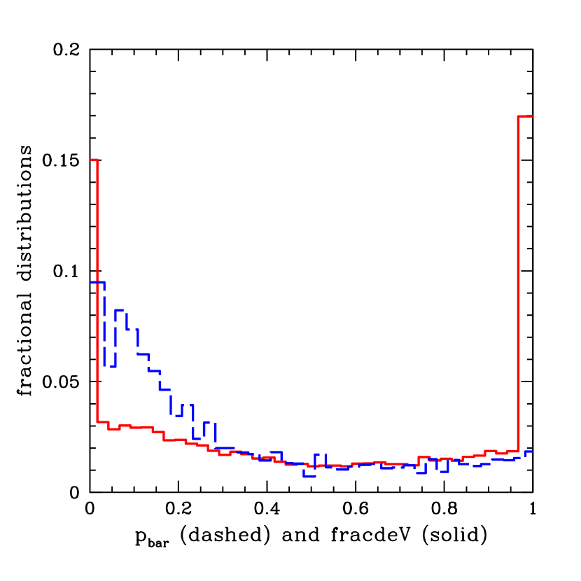
Figure 3: Distribution of bar likelihood ($p_{\mathrm{bar}}$, blue dashed histogram) and bulge strength (fracdeV, red solid histogram) of galaxies in the volume-limited catalogue. The histograms have been slightly offset from each other, for clarity.

The $p_{\mathrm{bar}}$ distribution is smooth, with most galaxies in the catalogue ($62\%$) having $p_{\mathrm{bar}}<0.3$. In contrast, the fracdeV distribution is peaked near 0 and 1; namely, most galaxies are either distinctly disc-dominated or bulge-dominated. Recall though that, because of our selection criteria, all of the bulge-dominated galaxies in the catalogue have spiral arms or discs (i.e., elliptical galaxies are excluded). We have tested that the clustering dependence of fracdeV is not very sensitive to its distribution: rescaling it to have a smoother distribution (such as that of $p_{\mathrm{bar}}$) yields clustering measurements within 5% of the results shown in the next section.

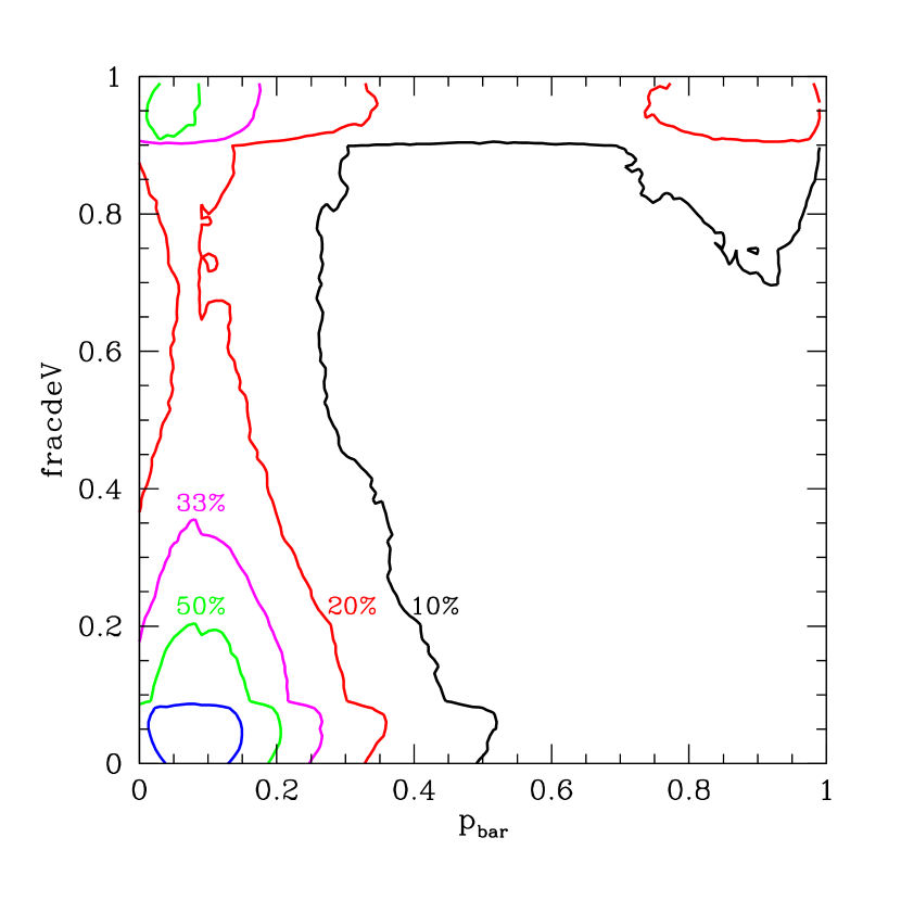
Figure 4: Distribution of $p_{\mathrm{bar}}$ versus fracdeV, with contours indicating 10, 20, 33, 50, and 75% of the maximum counts.

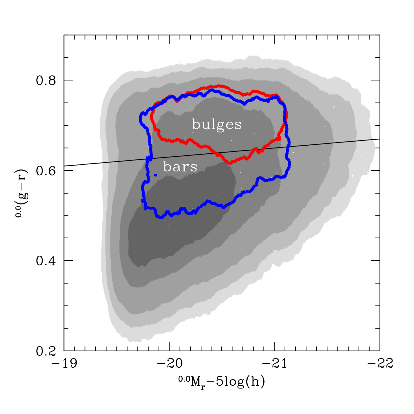
Figure 5: The optical colour-magnitude diagram (CMD), using extinction-corrected $g-r$ colour and $r$-band magnitude, with filled gray contours indicating 5, 10, 20, 50, and 75% of the maximum counts. The majority of the barred disc galaxies (with $p_{\mathrm{bar}}\geq 0.5$) and bulge-dominated disc galaxies (with fracdeV$\geq 0.9$) are indicated by the blue and red contours, respectively. $p_{\mathrm{bar}}\geq 0.5$ and fracdeV$\geq 0.9$ select a similar number of galaxies in the catalogue. The black line indicates the red sequence separator ($g-r=0.63-0.02\,(M_{r}-5\mathrm{log}(h)+20)$), used to identify red spirals in Masters et al. (2010b).

As discussed in Section 1, some authors have argued that the formation and evolution of bars and bulges could be related, depending on the type of bulge, gas content, and angular momentum distribution (e.g., Debattista et al. 2006; Laurikainen et al. 2007). Nevertheless, we find that $p_{\mathrm{bar}}$ and fracdeV are not simply, or monotonically, correlated, as can be seen from the distribution of $p_{\mathrm{bar}}$ versus fracdeV in Figure 4. We find that a large fraction of bulge-dominated galaxies are barred (in the upper right corner of the figure) and a large fraction are unbarred (upper left corner): for example, of those with fracdeV$>0.7$, $27\%$ have $p_{\mathrm{bar}}>0.7$ and $49\%$ have $p_{\mathrm{bar}}<0.3$. On the other hand, disc-dominated galaxies are mostly unbarred ($76\%$ of those with fracdeV$<0.3$ have $p_{\mathrm{bar}}<0.3$), and only a few per cent have bars—the lower right quadrant of the figure is empty. These results are consistent with M11, who showed that the bar fraction of disc galaxies increases with fracdeV, which is clearly the case for galaxies with $p_{\mathrm{bar}}>0.5$ on the right half of the figure.

We show the colour-magnitude distribution of the catalogue in Figure 5. Many of the galaxies in the catalogue are disc-dominated, and the majority of them are located in the “blue cloud”, the bluer mode of the bimodal colour distribution (e.g., Skibba 2009). Applying the colour-magnitude separator used for red spiral galaxies (Masters et al. 2010b; similar to that of S09), we find that only $31\%$ of the galaxies in the whole sample are on the red sequence, while $74\%$ of the bulge-dominated galaxies (fracdeV$\geq 0.9$, red contour) are on the red sequence (and are not highly inclined, so they are likely to have older stellar populations, rather than being dust reddened). Barred galaxies ($p_{\mathrm{bar}}\geq 0.5$, blue contour) have a much wider range of colours, with $48\%$ of them on the red sequence. In addition, barred galaxies have a bimodal colour distribution based on bar length, such that galaxies with longer bars are on the red sequence (Hoyle et al. 2011).

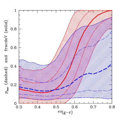
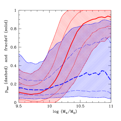
Figure 6: Left: $p_{\mathrm{bar}}$ (blue dashed line) and fracdeV (red solid line) as a function of $g-r$ extinction-corrected colour. Right: $p_{\mathrm{bar}}$ (blue dashed line) and fracdeV (red solid line) as a function of stellar mass. Running medians are shown as the thicker lines, the ${}^{1}/_{2}$-$\sigma$ range is shown by the thinner lines, and the hatched regions indicate the 1-$\sigma$ range between the 16 and 84 percentiles. As discussed in the text, $p_{\mathrm{bar}}$ and fracdeV appear to transition at a similar colour and mass scale: $g-r\approx 0.6$ and $M_{\ast}\approx 2\times 10^{10}\,M_{\odot}$.

Next, in Figure 6, we show the median (and ${}^{1}/_{2}$ and 1-$\sigma$ ranges) of $p_{\mathrm{bar}}$ and fracdeV as a function of colour and stellar mass. The majority of blue galaxies and low-mass galaxies are disc-dominated, while most red and massive galaxies are bulge-dominated. The bar probability is also positively correlated with colour and stellar mass, consistent with other studies (e.g., Sheth et al. 2008; Nair & Abraham 2010; M11), such that redder and more massive galaxies are more likely to have bars. Some studies have found a bimodal distribution of bars, such that blue, low-mass, or Sc/Sd-type galaxies also often have bars (Barazza et al. 2008; Nair & Abraham 2010), in contrast to our finding that the median $p_{\mathrm{bar}}<0.2$ at bluer colours and lower stellar masses. It is possible that in Galaxy Zoo, a large fraction of weak or short bars are missed in these galaxies.

Compared to the correlation with fracdeV, the correlations with $p_{\mathrm{bar}}$ in Figure 6 are not as strong and have more scatter, especially at the red and massive end. In other words, red and massive galaxies are more likely to have bars than blue and less-massive galaxies, but nonetheless there are many red and massive galaxies that lack bars. Either these galaxies never formed bars, or perhaps more likely, it is possible that they had bars in the past that were weakened (so that they are no longer detectable by GZ2) or destroyed; some galaxies may even have multiple episodes of bar formation in their lifetime (Bournaud & Combes 2002).

It is interesting that the transition from mostly unbarred to mostly barred galaxies and from disc-dominated to bulge-dominated galaxies occurs at similar colours and stellar masses. The colour transition occurs at extinction-corrected $g-r\approx 0.6$, in the “green valley” of the colour-magnitude distribution (e.g., Wyder et al. 2007), between the blue and red peaks of the distribution (see Figure 5). The stellar mass transition occurs at $M_{\ast}\approx 2\times 10^{10}\,M_{\odot}$, and is similar to the mass scale identified by Kauffmann et al. (2003; see also Schiminovich et al. 2007), above which galaxies have high stellar mass surface densities, high concentration indices typical of bulges, old stellar populations, and low star formation rates and gas masses.

5 Results: Clustering of Galaxies with Bars and Bulges

We now explore the environmental dependence of disc galaxies with bars and bulges by measuring marked projected correlation functions (described in Section 3). For the marks, we use $p_{\mathrm{bar}}$ and fracdeV, which indicate the presence or lack of a bar and bulge, respectively. We first present the total environmental dependence of these two galaxy properties in Section 5.1, and then we attempt to separate their environmental dependences in Section 5.2.

5.1 Environmental Correlations of Bar and Bulge Probability

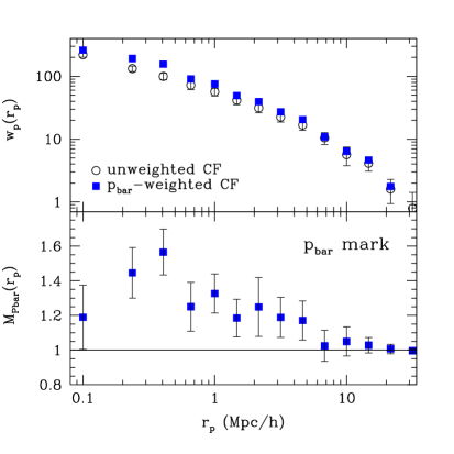
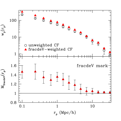
Figure 7: Upper panel: projected correlation function $w_{p}(r_{p})$ (circle points) and weighted projected correlation functions $W_{p}(r_{p})$. Lower panel: marked projected correlation functions, using $p_{\mathrm{bar}}$ mark (left) and fracdeV mark (right). Recall that the marked correlation function is defined as $M(r_{p})\equiv[1+W_{p}(r_{p})/r_{p}]/[1+w_{p}(r_{p})/r_{p}]$ (Eqn. 5).

In the upper panels of Figure 7, we show the projected clustering of the galaxies in our (disc-dominated) catalogue. In the lower panels, we show the the marked correlation functions, quantifying the environmental correlations of $p_{\mathrm{bar}}$ and fracdeV across a wide range of scales. The errors of the measurements are estimated using jack-knife resampling, and are analyzed in more detail in Appendix A. As noted in the appendix, a significant fraction of the error estimates is due to a single outlying jack-knife subsample.

We see a statistically significant environmental correlation in Figure 7 for both $p_{\mathrm{bar}}$ and fracdeV, which means that disc galaxies with bars and those with bulges tend to reside in denser environments on average. The environmental correlation is especially strong at small scales, at $r_{p}\leq 2\,\mathrm{Mpc}/h$. At these scales, the clustering signal is dominated by the “one-halo term” (pairs of galaxies within dark matter haloes), while at larger spatial scales the “two-halo term” (pairs of galaxies in separate haloes) dominates the clustering (e.g., Zehavi et al. 2004). In Section 5, we will interpret these correlation functions with the halo model of galaxy clustering (see Cooray & Sheth 2002 for a review).

It is important to quantify the statistical significance of the $M(r_{p})$ measurements, the degree to which they are inconsistent with unity. (A result of unity occurs when the weighted and unweighted correlation functions are the same, i.e., when the weight is not correlated with the environment.) Since the errors are correlated, the statistical significance should be quantified using the covariance matrices (see Eqn. 6 and Appendix A):

$$\sigma_{M}^{2}\,=\,(\boldsymbol{M}-\mathbf{1})^{T}\,\mathbf{Covar}^{-1}\,(\boldsymbol{M}-\mathbf{1}),$$ (7)

where $\boldsymbol{M}$ is the $p_{\mathrm{bar}}$ or fracdeV mark correlation function, and $\boldsymbol{M}-\mathbf{1}$ is its deviation from unity. (This is similar to the way one would compute the $\chi^{2}$ of a fit, where in this case a good “fit” with low $\sigma_{M}^{2}$ would be a measurement consistent with unity, or no environmental correlation). The $p_{\mathrm{bar}}$ and fracdeV mark correlation functions yield $\sigma_{M}^{2}=39.9$ and $43.4$, respectively, which could be interpreted as $6.3$ and $6.6\sigma$ significance for the marks. Note that this significance estimate is not highly dependent on the binning: narrower $r_{p}$ bins, for example, would yield more measurements with $M(r_{p})>1$, but they would have larger and more correlated errors.

The positive correlation at particular spatial separations $r_{p}$ implies that galaxies with larger values of $p_{\mathrm{bar}}$ and fracdeV tend to be located in denser environments at these scales. This is one of the main results of the paper. This can also be seen in the upper panels of the figures, in which the weighted correlation functions are larger than the unweighted ones.

The environmental dependence of bulges is not surprising; because of the “morphology-density relation”, in which dominant bulge components are associated with earlier-type morphologies, it is expected that bulge-dominated galaxies tend to be located in denser environments, in groups and clusters (e.g., Postman & Geller 1984; Bamford et al. 2009). Similar two-point clustering analysis have also clearly shown that bulge-dominated disc galaxies tend to be more strongly clustered than disc-dominated ones, on scales of up to a few Mpc (Croft et al. 2009; S09). Semi-analytic models, using stellar bulge-to-total ratios, have similarly predicted that bulge-dominated disc galaxies tend to form in more massive dark matter haloes (e.g., Baugh et al. 1996; Benson & Devereux 2010; De Lucia et al. 2011). Many theorists have argued that bulge formation is linked to minor and major galaxy mergers, and mergers and interactions tend to be more common in denser environments, especially in galaxy groups (e.g., Hopkins et al. 2009; Hopkins et al. 2010a; Martig et al. 2012); there is some observational evidence in favor of the link between bulges and mergers as well (e.g., Ellison et al. 2010).

On the other hand, one might not expect barred galaxies to be correlated with the environment, if bars form entirely by internal secular processes. Some recent studies have argued that barred and unbarred galaxies are located in similar environments, or have only weak evidence that barred galaxies are more strongly clustered at small scales (Marinova et al. 2009; Li et al. 2009; Barazza et al. 2009; Martínez & Muriel 2011; Wilman & Erwin 2012). Nevertheless, our volume-limited GZ2 catalogue is much larger than those of these studies (which except for Martínez & Muriel consist of $\sim 1000$ galaxies, or $\approx 1/17^{\mathrm{th}}$ as many as ours), and as stated in Section 3, an advantage of mark clustering statistics is that one can analyze the entire catalogue, without splitting it and without requiring a classification of “cluster”, “group”, and “field” environments. We are thus able to quantify the correlation between bars and the environment with greater statistical significance.

To test the effect of small number statistics, we performed a number of sparse sampling measurements (randomly selecting galaxies, or only selecting galaxies in small subregions or redshift slices of the sample). In general, we find that if fewer than $\sim 2000$ galaxies were used for our clustering measurements, we would not have a statistically significant detection of the environmental dependence of $p_{\mathrm{bar}}$, and the unmarked correlation functions would be too noisy. This may explain why previous studies of smaller galaxy catalogs did not detect a significant bar-environment correlation.

The $p_{\mathrm{bar}}$ marked correlation function in Figure 7, $M_{\mathrm{Pbar}}(r_{p})$, increases in strength with decreasing spatial separation. Such a trend is expected when the mark is positively correlated with the environment. An exception to this correlation occurs at small separations ($r_{p}\sim 100~{}\mathrm{kpc}/h$), where the result is consistent with no correlation at all. Fiber collisions could affect the lack of correlation at these scales, but at most $7\%$ of the targeted galaxies lack measured redshifts, and we obtain $M_{p_{\mathrm{bar}}}(100\,\mathrm{kpc}/h)\approx 1$ for all jack-knife subsamples, so this low mark correlation is likely a real effect. The weakening environmental correlation at small separations suggests that whatever conditions that make bars more likely at larger scales are removed in close pairs of galaxies. For example, close pairs are more likely to experience mergers, and bars may be weakened or destroyed immediately following merger activity, although new bars may form later (Romano-Díaz et al. 2008). Nonetheless, Marinova et al. (2009) and Barazza et al. (2009) find that bar fractions are slightly larger in cluster cores, although this is of weak statistical significance according to the authors. More recently, Nair & Ellison (in prep.) find that the bar fraction of disc galaxies decreases as pair separation decreases, consistent with our results.

It is interesting that $M_{\mathrm{Pbar}}(r_{p})$ peaks at approximately $400~{}\mathrm{kpc}/h$ (more precisely, the bin’s range is $316<r_{p}<525~{}\mathrm{kpc}/h$). Many of the galaxies contributing to the signal at these scales are likely “satellite” galaxies in groups, rather than the central galaxies. In fact, considering that these are disc galaxies and that $p_{\mathrm{bar}}$ is correlated with colour, it is likely that many of these are the same objects as the “red spirals” discussed in S09 (most of which have bars, according to Masters et al. 2010b; M11), a relatively large fraction of which are satellites ($f_{\mathrm{sat}}\approx 1/3$).

We also show (unmarked) clustering of barred versus non-barred galaxies ($p_{\mathrm{bar}}>0.2$ and $<0.2$), and bulge-dominated versus disc-dominated ones (fracdeV$>0.5$ and $<0.5$), in the upper panels of Figure 8. At large scales ($r_{p}>2\,\mathrm{Mpc}/h$), their clustering strength is the same. At smaller separations, however, barred galaxies tend to be more strongly clustered than unbarred ones and bulge-dominated galaxies tend to be more strongly clustered than disc-dominated ones. The scale at which the correlation functions diverge corresponds to the scale of the transition from the “one-halo term” (pairs of galaxies within haloes) to the “two-halo term” (galaxies in separate haloes). These clustering measurements then suggest that barred and unbarred galaxies may reside in the same dark matter haloes, but the former are more likely to be central galaxies than the latter. The same applies for the presence/absence of bulges in central/satellite galaxies. We will return to this issue when we apply halo occupation modeling to the measured correlation functions, in Section 6.3.

5.2 Disentangling the Environmental Correlations

As we have shown in previous sections, disc galaxies with large bulges are more likely to have a bar (see Fig. 4). We have also shown that both bulge-dominated discs and discs with bars are more strongly clustered than average (Fig. 7). We address in this Section the question of whether one of these two galaxy properties is more dependent on the environment, or whether their environmental correlations are independent. That is to say, we will determine whether bulge-dominated galaxies with bars are more strongly clustered than bulge-dominated galaxies without bars, and whether barred galaxies with bulges are more strongly clustered than barred galaxies with no or small bulges.

In addition, we know that disc galaxies hosting bars tend to be redder and have higher stellar masses than those with weak or no bars (Fig. 6). We will later address in Section 6.1 whether the environmental correlations of galaxy colour or stellar mass (e.g., Skibba & Sheth 2009; Li & White 2009) can account for the environmental correlation we have observed of bars.

In the lower panels of Figure 8, we show the $p_{\mathrm{bar}}$ mark correlation functions for bulge-dominated and disc-dominated galaxies (fracdeV$>0.5$ and $<0.5$), as well as the fracdeV mark correlation functions for barred and unbarred galaxies ($p_{\mathrm{bar}}>0.2$ and $<0.2$). Using the fracdeV$>0.5$ threshold, $44\%$ of our (disc) galaxy catalogue is bulge-dominated, and using $p_{\mathrm{bar}}>0.2$, $49\%$ of it is barred. Following the procedure described in the appendix of S09, the mark correlations are shown when the marks are rescaled so that they have the same distribution as that of the whole sample (see Fig. 3). Such a rescaling is necessary in order to compare the mark correlation functions. (In this case, the mark correlation measurements are similar, within $\sim$10%, when the mark distributions are not rescaled.)

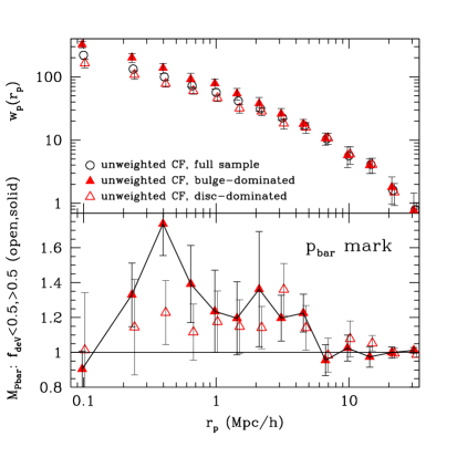
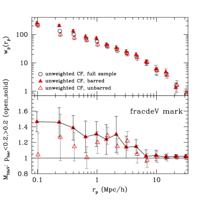
Figure 8: Left plot, lower panel: $p_{\mathrm{bar}}$ mark correlation functions with fracdeV$<0.5$ (disc-dominated; open triangle points) and $>0.5$ (bulge-dominated; solid triangles). Right plot, lower panel: fracdeV mark correlation functions with $p_{\mathrm{bar}}<0.2$ (unbarred; open triangles) and $>0.2$ (barred; solid triangles); the split is done at 0.2 in order to have a similar number of galaxies in each subsample. Mark distributions have been rescaled to match distribution of whole sample (Fig. 3). For clarity, the points are slightly offset from each other, and the points are connected for bulge-dominated and barred galaxies, to guide the eye. Upper panels show the (unweighted) correlation functions, for the full sample (same as in Fig. 7) and the subsamples, indicated by the legends in the figures.

The $p_{\mathrm{bar}}$ and fracdeV mark correlation functions are all still above unity, but they are statistically significant only for bulge-dominated (fracdeV$>0.5$) and barred ($p_{\mathrm{bar}}>0.2$) galaxies, respectively. Using Eqn. 7, these $p_{\mathrm{bar}}$ and fracdeV mark correlations both have a statistical significance of $6\sigma$. In other words, bulge-dominated galaxies exhibit a significant bar-environment correlation, and barred galaxies exhibit a bulge-environment correlation. Considering that these residual environmental correlations are so significant, it appears that the environmental dependencies of barred and bulge-dominated galaxies are somewhat independent of each other: the bar-environment correlation is not due to the bulge-environment correlation, and vice versa. (The environmental dependencies of bars and pseudo-bulges, however, may be more closely related, as discussed in the introduction.) Lastly, we point out that though S0s are to some extent environmentally dependent (Hoyle et al. 2011; Wilman & Erwin 2012), they are not likely to be driving the bar-environment correlation in the left panels of Fig. 8. S0s do not have a particularly large bar fraction compared to their spiral counterparts (Laurikainen et al. 2009; Buta et al. 2010), and their bar fraction does not exhibit a significant environmental dependence (Barway et al. 2011; Marinova et al. 2012).

6 Interpretation of the $p_{\mathrm{bar}}$-environment correlation

In the previous section, we quantified the environmental dependence of barred galaxies, using projected clustering measurements with the largest catalogue of galaxies with bar classifications to date. Here we perform tests and analyses of these results, in order to better understand the origin of these environmental correlations.

We also quantified the environmental dependence of galaxy bulges, but as stated in Section 5.1, this has been thoroughly studied already and is closely related to the morphology-density relation. Furthermore, the colour and stellar mass dependence of the morphology-density relation has been studied elsewhere (e.g., Kauffmann et al. 2004; Blanton et al. 2005; Park et al. 2007; van der Wel et al. 2010), including with Galaxy Zoo data (Bamford et al. 2009; Skibba et al. 2009), so we will not study it further here.

In Section 6.1, we examine the stellar mass and colour dependence of the measured $p_{\mathrm{bar}}$-environment correlation. Then in Section 6.2, we use mock galaxy catalogues to predict the strength of the $p_{\mathrm{bar}}$-environment correlation if it were entirely due to redder galaxies occupying more massive dark matter haloes. Lastly, we apply halo occupation models to the clustering of barred and unbarred galaxies in Section 6.3.

6.1 Dependence of the environmental correlation on stellar mass and colour

The probability of a galaxy being barred is correlated with its stellar mass (see Fig. 6b; Nair & Abraham 2010), so it is important to ask whether the environmental dependence of barred galaxies measured in Section 5.1 is due to the environmental dependence of stellar mass. Li et al. (2009) argue that in their catalogue, at fixed stellar mass, the projected clustering of barred and unbarred galaxies is similar. With a much larger volume-limited catalogue, we can now analyze the stellar mass and colour dependence with greater accuracy.

6.1.1 Mark shuffling test

Rather than splitting our catalogue by stellar mass and then measuring the $p_{\mathrm{bar}}$ mark correlation function of the subcatalogues, we can take better advantage of the number statistics with a different test. Our procedure is as follows. We randomly shuffle the $p_{\mathrm{bar}}$ marks at a given stellar mass, and then repeat the clustering measurement. The distribution $p(p_{\mathrm{bar}}|M_{\ast})$ does depend on stellar mass, but there is substantial scatter, so it is unclear a priori what the resulting mark correlation function would look like. The result can be directly compared to the original measurement (Fig. 7a), because by merely shuffling the marks we are not changing the overall mark distribution. If the resulting mark correlation function is similar to the original (unshuffled) one, then this could be interpreted as evidence that the $p_{\mathrm{bar}}$ mark correlation is due to the environmental correlation of stellar mass. If the resulting mark correlation is weak but significant, then the environmental correlation is partly due to stellar mass, and if there is no mark correlation, then it is not due to stellar mass at all.

We performed this test using ten bins of stellar mass (of width 0.15 dex), and the result yields no significant environmental correlation, as shown in Figure 9a (open triangles in the lower panel). Shuffling by stellar mass appears to nearly completely wash out the correlation, as $M_{p_{\mathrm{bar}}}$ is consistent with unity in every $r_{p}$ bin. Note, however, that the stellar mass uncertainties are comparable or larger than the bin widths, which could artificially weaken the correlation.

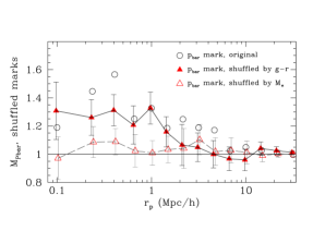
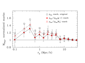
Figure 9: Left: $p_{\mathrm{bar}}$ mark correlation function, shuffled as a function of $g-r$ colour (solid triangles) and stellar mass (open triangles). Right: $p_{\mathrm{bar}}/\langle p_{\mathrm{bar}}|g-r\rangle$ mark (solid triangles) and $p_{\mathrm{bar}}/\langle p_{\mathrm{bar}}|M_{\ast}\rangle$ mark (open triangles) correlation functions. For comparison, the original $p_{\mathrm{bar}}$ mark correlation function is also shown (open circles, same as Fig. 7a). Ten bins were used, most with $\sim$1000-1400 galaxies/bin; using fewer or more bins yields similar results. The unweighted correlation function (upper panel in previous two figures) is omitted, because the full sample is used for all three mark correlation measurements.

We have also performed the same test by shuffling the $p_{\mathrm{bar}}$ marks as a function of $g-r$ colour (see the distribution in Fig. 6a), and in this case, the $p_{\mathrm{bar}}$ mark correlation (solid triangles in Fig. 9a) is nearly as strong as the original mark correlation measurement. This suggests that the environmental dependence of colour partially explains that of $p_{\mathrm{bar}}$. The colour-shuffled correlation function does not reproduce either the upturn at $400~{}\mathrm{kpc}/h$ or the downturn at $100~{}\mathrm{kpc}/h$; however, we attribute this to the shuffling process.

By taking the ratio of the marked correlation functions in Figure 9a, we can make an approximate estimate of the fraction of the environmental dependence of $p_{\mathrm{bar}}$ that is accounted for by colour and stellar mass. In particular, we use all of the jack-knife subsamples (not just the measurements in the figure) to estimate this as robustly as possible, and we use the mean and variance of the ratio $(M^{\prime}-1)/(M_{P\mathrm{bar}}-1)$, where $M^{\prime}$ is either the colour-shuffled or mass-shuffled mark correlation function. We use the measurements over the range $0.1\leq r_{p}\leq 2.2~{}\mathrm{Mpc}/h$, which encompasses the environmental correlations within dark matter haloes. We find that colour accounts for $60\pm 10~{}\%$ of the environmental dependence of $p_{\mathrm{bar}}$, while stellar mass accounts for only $15\pm 2~{}\%$. This suggests that the environmental dependence of colour explains the majority, but not all, of the environmental dependence of bars. Our results are not consistent with Lee et al. (2012a), who claim that the environmental dependence of bars disappears at fixed colour or central velocity dispersion, and the disagreement may be due to their use of different bar classifications and environment measures; in addition, lenticular galaxies are excluded from their sample, but not from ours.

6.1.2 Normalized mark test

It is possible that the contribution from stellar mass is larger than estimated above, because the masses have larger uncertainties than the colours. To address this, we perform another test of the stellar mass and colour contribution to the bar-environment correlation, which does not involve binning these parameters. The purpose of this test is to remove the environmental dependence of stellar mass or colour (see e.g. Cooper et al. 2010), and consequently assess the strength of the residual environmental dependence of $p_{\mathrm{bar}}$.

Our procedure is as follows. For every galaxy, the $p_{\mathrm{bar}}$ mark is normalized by the mean $p_{\mathrm{bar}}$ of galaxies with that stellar mass (i.e., we use $p_{\mathrm{bar}}/\langle p_{\mathrm{bar}}|M_{\ast}\rangle$ as the mark). Note that the mean is slightly larger than the median, which is plotted in Figure 6, and is similarly a smooth function of stellar mass, so this normalization is not sensitive to the mass uncertainties. Then the mark distribution is rescaled so that it matches the overall $p_{\mathrm{bar}}$ distribution (as was done in Sec. 5.2), because consistent mark distributions are required in order to compare mark correlations. Now the new mark correlation function is measured, and can be compared to the original one. With this test, if the mark correlation function were close to unity, it would mean that $M_{\ast}$ accounts for most of the environmental correlation. The same test is also done to assess the contribution of the $g-r$ colour-environment correlation, with the analogous $p_{\mathrm{bar}}/\langle p_{\mathrm{bar}}|g-r\rangle$ mark.

The result is shown in Figure 9b. The colour-normalized mark correlation function is closer to unity, and therefore accounts for more of the bar-environment correlation. As in the previous section, we can estimate the relative contribution of colour and mass to this correlation, now using the ratio $(M_{P\mathrm{bar}}-M^{\prime})/(M_{P\mathrm{bar}}-1)$, where $M^{\prime}$ is the colour- or mass-normalized mark correlation function. This yields an estimate of $60\pm 5~{}\%$ of the bar-environment correlation accounted for by colour, consistent with the mark shuffling test in Section 6.1.1. Stellar mass now accounts for $25\pm 10~{}\%$, a larger contribution than estimated above, but still less significant than colour. We conclude that the environmental dependence of $p_{\mathrm{bar}}$ is not primarily due to that of stellar mass.

Perhaps more than stellar mass, the colour is a better tracer of star formation (and dust content) in disc galaxies, which in turn is expected to be related to the likelihood of the galaxies having a bar (e.g., Scannapieco et al. 2010; Masters et al. 2010b). Redder disc galaxies with older stellar populations and in more massive haloes are more likely to have formed a stable bar; however, mergers/interactions can disrupt a bar, which could explain why the original $p_{\mathrm{bar}}$ mark correlation function (circle points in Fig. 9), unlike the colour-shuffled one, turns toward unity at small separations.

6.2 Colour dependence in mock galaxy catalogues

To add to the interpretation of the colour dependence of the $p_{\mathrm{bar}}$-environment correlation in the previous section, we analyze the clustering of galaxies in a mock galaxy catalogue, in which we add bar likelihoods with a prescription based on galaxy colour.

We use the mock catalogue of Muldrew et al. (2012), which was constructed by populating dark matter haloes of the Millennium Simulation (Springel et al. 2005) using the halo occupation model of Skibba & Sheth (2009). The catalogue reproduces the observed luminosity function, colour-magnitude distribution, and the luminosity and colour dependence of galaxy clustering in the SDSS (Skibba et al. 2006; Skibba & Sheth 2009). Central galaxies in haloes are distinguished from satellite galaxies, which are distributed around them and are assumed to follow a Navarro, Frenk & White (1996) profile with the mass-concentration relation from Macciò, Dutton & van den Bosch (2008).

For the purposes of this work, which is focused on disc galaxies, we construct a sub-catalogue from this mock, by selecting galaxies from the colour-magnitude distribution. In particular, we first select galaxies with $M_{r}-5\mathrm{log}(h)\leq-19.4$. We require that the luminosity function is consistent with the data. (Since the catalogue was constrained with absolute magnitudes $K$-corrected to $z=0.1$, we use the ${}^{0.1}M_{r}$ luminosity function.) We randomly select galaxies (independently of halo mass or central/satellite status) in absolute magnitude bins until the consistent luminosity function is obtained. Secondly, we similarly require that the colour-magnitude distribution, $p(g-r|M_{r})$, is consistent with the data, using bins of 0.25 mag (see e.g. Skibba & Sheth 2009). The selection of disc galaxies in the GZ catalogue means that the red sequence is under-represented (M11). Finally, we use $p(p_{\mathrm{bar}})$ (Fig. 3), and $p(p_{\mathrm{bar}}|g-r)$ (Fig. 6) distributions to generate “$p_{\mathrm{bar}}$” for the mock galaxies. That is, we assume that the environmental dependence of $p_{\mathrm{bar}}$ is due to that of $g-r$ colour, which in turn is due to more massive haloes in dense environments.

We can now measure the projected correlation function and $p_{\mathrm{bar}}$ marked correlation function of the mock catalogue, in order to compare to the GZ measurements in Figure 7. The result (averaged over eight realizations) is shown in Figure 10. As with the observational measurements, the errors are estimated using jack-knife resampling; the variance of the eight mocks is much smaller. If we were to apply the observed errors instead (and account for the different size of the GZ and mock catalogues), we obtain similar error bars at large scales but smaller ones at small scales ($r_{p}<\mathrm{few}\,\mathrm{Mpc}/h$).

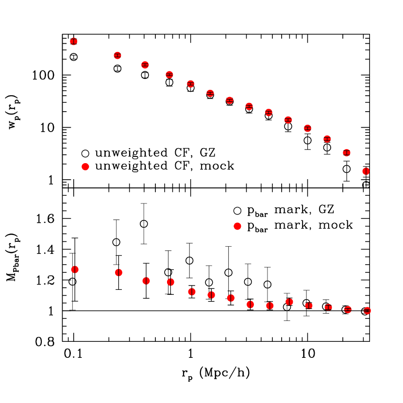
Figure 10: Clustering comparison between the Galaxy Zoo and mock catalogues. Solid red circles indicate the projected correlation function and mark correlation function of the mock catalogue, using $p_{\mathrm{bar}}(g-r)$ as the mark (see distribution in Fig. 6a, and text for details). For comparison, the original GZ measurements are also shown here (open circles, same as Fig. 7a); the points are slightly offset in the lower panel, for clarity.

In the upper panel, the discrepancy between these projected correlation functions at large scales has been previously observed and is not statistically significant (see Zehavi et al. 2005; Skibba et al. 2006); it is likely due to cosmic variance. The discrepancy at small scales, however, is significant. The fact that the correlation functions are consistent at scales of $r_{p}\geq 1\,\mathrm{Mpc}/h$, but the small-scale clustering of the GZ catalogue is suppressed, could mean that the satellite distribution as a function of halo mass is slightly different in the real universe, and is not reproduced with the colour-magnitude selection procedure.

The $p_{\mathrm{bar}}(g-r)$ mark correlation function of the mock is weaker than the GZ measurement, but similar to the ($g-r$)-shuffled mark measurement in Figure 9a. This suggests that part, but not all, of the environmental dependence of $p_{\mathrm{bar}}$ is due to more massive haloes hosting redder galaxies, which are more likely than average to be barred. By taking the ratio of the marked correlation functions, $(M_{\mathrm{mock}}-1)/(M_{\mathrm{GZ}}-1)$, we estimate that the colour-halo mass correlation accounts for $50\pm 10~{}\%$ of the environmental dependence of $p_{\mathrm{bar}}$, which is slightly lower than, but consistent with the estimate in Section 6.1; conversely, the rest (also $50\pm 10~{}\%$) is due to other processes unrelated to colour or stellar mass, perhaps involving the gas content (see Masters et al. 2012) or angular momentum distribution.

Also note that, as in Figure 9, the $p_{\mathrm{bar}}(g-r)$ mark correlation function in Figure 10 lacks a drop in strength at $r_{p}\sim 100\,\mathrm{kpc}/h$, which we see in the original clustering measurement. This implies that, in the real universe, although galaxies at small separations (usually center-satellite galaxy pairs) tend to be redder in more massive haloes, this does not entail a higher bar fraction; the lack of a $p_{\mathrm{bar}}$-environment correlation at small separations in Figure 7a is not related to galaxy colour.

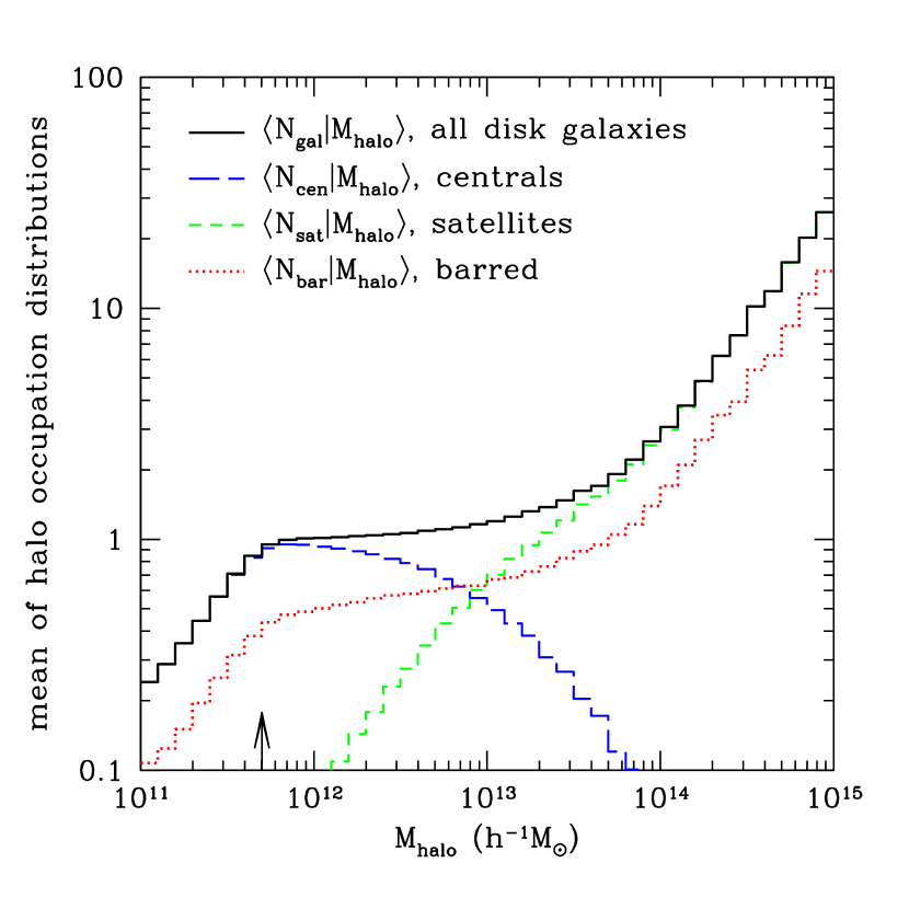
Figure 11: Mean of halo occupation distributions in the mock catalogue. Black solid histogram: mean occupation number of all (colour-magnitude selected) disc galaxies in the mock; blue dashed histogram: mean occupation number of central galaxies; green short-dashed histogram: mean occupation number of satellite galaxies. The peak of the halo mass distribution is indicated by the arrow. The red dotted histogram shows the mean occupation number for galaxies with $p_{\mathrm{bar}}>0.2$ (where the bar likelihood is computed from the $p(p_{\mathrm{bar}}|g-r)$ distribution), which are a combination of central galaxies in low-mass haloes and satellites in massive haloes. A larger $p_{\mathrm{bar}}$ threshold yields a lower $\langle N_{\mathrm{bar}}|M_{\mathrm{halo}}\rangle$, but of similar shape.

Finally, we have computed the halo mass distribution and halo occupation distribution of galaxies in the mock catalogue. The halo occupation distribution (HOD) is the number distribution of galaxies occupying haloes of a given mass, and of particular importance for galaxy clustering is the mean occupation function, $\langle N|M\rangle$ (which is described further in Section 6.3). The mean occupation functions of galaxies in the mock are shown in Figure 11. The mock galaxies are mostly hosted by haloes with masses $M_{\mathrm{vir}}\geq 4\times 10^{11}\,h^{-1}\,M_{\odot}$; there are fewer haloes less massive than this, due to the luminosity threshold ($M_{r}=-19.4$). The central galaxy HOD drops off at high masses because the central galaxies of these haloes rarely meet the CMD selection criteria of our GZ catalogue; to wit, many centrals in massive haloes are elliptical, not disc, galaxies (Skibba et al. 2009; Guo et al. 2009; De Lucia et al. 2011). Satellite galaxies dominate in number at masses of $M_{\mathrm{vir}}\geq 10^{13}\,h^{-1}\,M_{\odot}$. In the mock, the “barred” galaxies (determined from the $p(p_{\mathrm{bar}}|g-r)$ distribution), indicated by the dotted histogram, consist of a combination of central galaxies in low-mass haloes and satellites in massive haloes. The fraction of barred galaxies in the mock is not strongly halo mass dependent, but it is highest between $10^{12.5}<M_{\mathrm{vir}}<10^{14.3}\,h^{-1}\,M_{\odot}$, in the haloes that typically host galaxy groups. The HOD statistics of the mock catalogue will be compared to the results of halo occupation modeling, in the following section.

6.3 Halo occupation modeling of the clustering measurements

In this section, complementary to the mock catalogue analysis of the previous section, we apply dark matter halo models to the measured projected correlation functions, $w_{p}(r_{p})$, of the whole volume-limited sample of (disc) galaxies, and of the subsamples of barred and unbarred galaxies, plotted in the upper panels of Figure 7 and Figure 8b. Since there are only small differences between these measurements for barred and unbarred galaxies, one can expect small differences between the well-fitting models. The purpose of the halo model analysis is to constrain the types of haloes that host barred and unbarred disc galaxies.

We use a halo occupation model of galaxy clustering, (e.g., Zheng et al. 2007; Zehavi et al. 2011), in which the halo occupation distribution, $P(N|M)$, of central and satellite galaxies depends on halo mass, $M$, and the luminosity threshold, $L_{\mathrm{min}}$. In this case the luminosity threshold is $M_{r}\leq-19.4$, corresponding to an approximate halo mass threshold of $M_{\mathrm{min}}\approx 4-5\times 10^{11}\,h^{-1}\,M_{\odot}$ (which is consistent with the mock catalogues in Section 6.2).

Haloes of mass $M$ are occupied by $N_{\mathrm{gal}}$ galaxies, consisting of a single central galaxy and $N_{\mathrm{sat}}$ satellite galaxies, such that the mean occupation function is described as the following:

$$\langle N_{\mathrm{gal}}|M,L_{\mathrm{min}}\rangle\,=\,\langle N_{\mathrm{cen}}|M,L_{\mathrm{min}}\rangle\,\Bigl{[}1+\langle N_{\mathrm{sat}}|M,L_{\mathrm{min}}\rangle\Bigr{]}$$ (8)

where,

$$\langle N_{\mathrm{cen}}|M\rangle\,=\,\frac{1}{2}\Biggl{[}1\,+\,\mathrm{erf}\Biggl{(}\frac{\mathrm{log}(M/M_{\mathrm{min}})}{\sigma_{\mathrm{log}M}}\Biggr{)}\Biggr{]}$$ (9)

and

$$\langle N_{\mathrm{sat}}|M\rangle=\Biggl{(}\frac{M-M_{0}}{M_{1}^{{}^{\prime}}}\Biggr{)}^{\alpha}.$$ (10)

In practice, we account for the fact that there is significant scatter in the relation between central galaxy luminosity and halo mass, and that the satellite halo occupation function drops off more rapidly than a power-law at low masses just above $M_{\mathrm{min}}$. See Appendix A2 of Skibba & Sheth (2009) for details.

We will also use the halo occupation models to compare the fraction of satellite galaxies of barred and of unbarred galaxies. The satellite fraction is given by

$$f_{\mathrm{sat}}\,=\,\frac{\int_{M_{\mathrm{min}}}dM\,(dn/dM)\,\langle N_{\mathrm{sat}}|M\rangle}{\int_{M_{\mathrm{min}}}dM\,(dn/dM)\,(\langle N_{\mathrm{cen}}|M\rangle+\langle N_{\mathrm{sat}}|M\rangle)},$$ (11)

where $dn/dM$ is the halo mass function (Sheth & Tormen 1999; Tinker et al. 2008b). Note that we will not attempt to account for the fact that central galaxies in massive haloes will often not meet the selection criteria for disc galaxies, because these galaxies will be dominated in number by satellites (see Fig. 11), whose abundance we can constrain.

In Figure 12, we show the results of the halo occupation modeling, applied to the whole catalogue and to the subsamples of barred and unbarred galaxies.

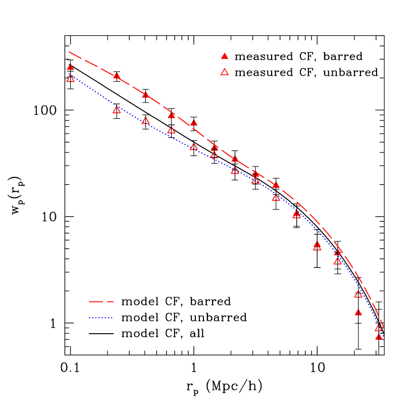
Figure 12: Halo occupation models of clustering of all galaxies in the sample (solid black curve), the barred subsample of galaxies (red dashed curve), and the unbarred subsample (blue dotted curve). The corresponding measured correlation functions are also shown, for barred and unbarred galaxies (solid and open triangle, respectively).

The parameters of these HOD models are listed in Table 1. We fixed the parameters $\sigma_{\mathrm{log}M}=0.26$ and $M_{0}=10^{11.60}M_{\odot}/h$, because they are not constrained well by HOD models of clustering (see Zheng et al. 2007; Zehavi et al. 2011); $\sigma_{\mathrm{log}M}$, which quantifies the scatter between central galaxy luminosity and halo mass, can be constrained by satellite kinematics and the conditional luminosity function (More et al. 2009; Cacciato et al. 2009).

sample	log $M_{\mathrm{min}}/h^{-1}M_{\odot}$	$M_{1}^{{}^{\prime}}/M_{\mathrm{min}}$	$\alpha$
all	$11.65\pm 0.05$	$16.0\pm 1.0$	$0.90\pm 0.04$
barred	$11.65\pm 0.05$	$16.0\pm 1.0$	$0.95\pm 0.06$
unbarred	$11.65\pm 0.05$	$19.0\pm 1.0$	$0.80\pm 0.06$

Table 1: Halo occupation distribution parameters for the model (8-10) fitted to the clustering measurements of the whole sample and the barred and unbarred subsamples, shown in Fig. 12.

As stated above, the halo mass threshold of the three measurements is the same. Nonetheless, because of differences in the small-scale clustering, there are differences in the satellite HOD, $\langle N_{\mathrm{sat}}|M\rangle$ (Eqn. 10). In particular, firstly, the fraction of satellite galaxies varies. The whole catalogue has $f_{\mathrm{sat}}\approx 23\%$, consistent with the mock catalogue analysis in Section 6.2, which yielded a similar fraction (also $\approx 23\%$). For comparison, the barred and unbarred subsamples have $f_{\mathrm{sat}}\approx 25\%$ and $20\%$, respectively.

Secondly, the key difference between the well-fitting models for the barred subsample is that they have a steeper slope $\alpha$ (compared to the slope for the full sample and for unbarred galaxies), which means that the larger satellite fraction of barred galaxies is due to more satellites in more massive haloes. In contrast, the well-fitting models for the unbarred subsample have a shallower slope, so not only is the unbarred sample dominated by central galaxies in lower mass haloes, but the small fraction of unbarred satellites is not in the most massive haloes either.

7 Conclusions and Discussion

We selected a volume-limited catalogue of 15810 nearly face-on disc galaxies in the SDSS, which have visual morphology classifications from Galaxy Zoo 2. We analyzed the properties of galaxies with bars and bulges, characterizing bar and bulge likelihood with the $p_{\mathrm{bar}}$ and fracdeV parameters. Using “marked” two-point correlation functions, we quantified the environmental dependence of bar and bulge likelihood as a function of the projected separation between galaxies.

To conclude, the following are the main results of our paper:

• Correlations of bars and bulges with colour and stellar mass: We find a strong correlation between the bar likelihood ($p_{\mathrm{bar}}$) and optical colour and stellar mass, such that redder and more massive disc galaxies are up to twice as likely to have bars than their bluer low-mass counterparts, although there is considerable scatter in the correlation, especially at the red (high-mass) end. We find similar correlations with bulge strength (fracdeV), but with less scatter. The quantities $p_{\mathrm{bar}}$ and fracdeV appear to have a transition at the same stellar mass and colour ($M_{\ast}\approx 2\times 10^{10}\,M_{\odot}$, $g-r\approx 0.6$).

• Environmental dependence of bars and bulges: We clearly detect and quantify the environmental dependence of barred galaxies and of bulge-dominated galaxies, such that barred and bulge-dominated disc galaxies tend to be found in denser environments than their unbarred and disc-dominated counterparts. In particular, by analyzing $p_{\mathrm{bar}}$ and fracdeV marked correlation functions, we obtained environmental correlations that are statistically significant (at a level of ${>6}\sigma$) on scales of 150 kpc to a few Mpc. From sparse sampling tests with our catalogue, we argue that the small number statistics of previous studies inhibited their detection of a bar-environment correlation.

• Contribution from colour and stellar mass to bar-environment correlation: By accounting for the environmental dependence of colour and stellar mass, we argue that they contribute approximately $60\pm 5~{}\%$ and $25\pm 10~{}\%$, of the $p_{\mathrm{bar}}$-environment correlation, respectively. From a similar analysis of a mock galaxy catalogue, we argue that the environmental dependence of $p_{\mathrm{bar}}$ appears to be partially ($50\pm 10~{}\%$) due to the fact that redder galaxies, which are often barred, tend to be hosted by more massive haloes. Conversely, up to half of the bar-environment correlation is not due to colour or stellar mass, and must be due to environmental influences or to another independent parameter (possibly gas content, or angular momentum distribution).

• Halo model analysis of clustering of barred galaxies: Our analyses with a mock galaxy catalogue and halo occupation models suggest that barred galaxies are often either central galaxies in low-mass dark matter haloes ($M\sim 10^{12}\,M_{\odot}$) or satellite galaxies in more massive haloes ($M\sim 10^{13-14}\,M_{\odot}$, hosting galaxy groups).

We argue that the environmental dependence of galaxy colours can account for approximately a half ($50\pm 20~{}\%$) of the environmental correlation of $p_{\mathrm{bar}}$. The optical colours are correlated with star formation rate and age, as well as gas and dust content, all of which may be related to the presence of disc instabilities such as bars. We find that a galaxy’s stellar mass and bulge component, on the other hand, do not appear to be strongly related to its likelihood of having a bar. This suggests that it is primarily older disc galaxies with lower star formation rates (which often reside in denser environments) that are able to form and maintain a stellar bar (see Masters et al. 2010b).

Conversely, this means that the remaining half of the environmental correlation of $p_{\mathrm{bar}}$ is not explained by the environmental dependence of colour or stellar mass, suggesting that bar formation (or the lack of bar destruction) is likely influenced by the galaxy’s environment, in addition to the effects described above. Bulge formation, which is to some extent independently correlated with the environment (see Section 5.2), is also expected to be affected by interactions and merger activity (Hopkins et al. 2009; Kannan et al., in prep.).

During the final stages of this work, Martínez & Muriel (2011) in a related study found that the bar fraction does not significantly depend on group mass or luminosity, or on the distance to the nearest neighbour. Their sample is smaller than ours, however, and is apparent magnitude-limited rather than volume-limited. In addition, they use bar classifications from Nair & Abraham (2010), which include somewhat weaker bars than Galaxy Zoo 2 (see M11), which are bars that tend to be found in bluer galaxies (and hence in less dense environments). In another recent paper, Lee et al. (2012a) also analyze the environmental dependence of bars, using bar classifications consistent with Nair & Abraham (2010), and claim that the bar fraction does not depend on the environment at fixed colour or central velocity dispersion, contrary to our results. However, a crucial difference between these two analyses and ours is that they use environment measures that mix environments at different scales, while we analyze the environmental correlations as a function of galaxy separation.

A particularly interesting result of this paper is the scale dependence of the environmental correlations of bar and bulge likelihood (see Fig. 7, Sec. 5). Environmental correlations should be interpreted differently at different scales (Blanton & Berlind 2007; Wilman et al. 2010; Muldrew et al. 2012), as galaxies at small separations ($r_{p}<2~{}\mathrm{Mpc}/h$) are often hosted by the same dark matter halo, while galaxies at larger separations are often hosted by separate haloes. We see that more massive haloes, which tend to reside in relatively dense environments, tend to host more disc galaxies with bars and bulges.

Moreover, the $p_{\mathrm{bar}}$-environment correlation peaks at $r_{p}\sim 400~{}\mathrm{kpc}/h$, which suggests that many barred galaxies are central or satellite galaxies in groups and clusters. That is, some aspect of group environment triggers the formation of bars, in spite of the fact that bars are often thought to form by internally driven secular processes (e.g., Kormendy & Kennicutt 2004). Secular processes may sometimes be externally driven. For example, cosmological simulations predict that tidal interactions with dark matter substructures, which are common in such environments, could induce bar formation and growth (Romano-Díaz et al. 2008; Kazantzidis et al. 2008). On the other hand, the $p_{\mathrm{bar}}$-environment correlation is not significant for closer pairs, suggesting that the enhanced likelihood of galaxies being barred is erased if the galaxies are merging with each other; however, this measurement at small separations ($r_{p}<100~{}\mathrm{kpc}/h$) has large uncertainty and may be affected by fiber collisions (see Sec. 2.4), so it should be viewed with caution. Analyses of bars in close pairs of galaxies (e.g., Nair & Ellison, in prep.) could shed more light on this issue.

In general, we can at least conclude that group environments increase the likelihood of bar formation in disc galaxies. Minor mergers and interactions are relatively common in galaxy groups (Hopkins et al. 2010b), and tidal interactions with neighboring galaxies can trigger disc instabilities and subsequent bar formation (Noguchi 1996; Berentzen et al. 2004); there is observational evidence for this as well (Elmegreen et al. 1990; Keel et al. 1996). Tidal interactions can also affect the bar’s pattern speed and other properties (Miwa & Noguchi 1998). The evolution of barred galaxies in group environments and in minor mergers/interactions is clearly in need of further study.

Considering that bar formation does appear to depend on the host galaxy’s environment, and that bars form by secular evolution, our results suggest that the dichotomy between internal secular processes and external environmental processes is not as strict as previously thought. It is possible that some structural changes in galaxy discs may be triggered or influenced by the galaxy’s environment. For example, Kormendy & Bender (2012) recently argued that, “harassment”, the cumulative effect of encounters with satellite galaxies, may influence secular evolution. Furthermore, “strangulation”, in which the hot diffuse gas around newly accreted satellites is stripped, removes the fuel for future star formation (Larson et al. 1980), and could contribute to more stable or growing bars (Berentzen et al. 2007; Masters et al. 2012).

In addition, our results could also indicate a link between bars and active galactic nuclei (AGN) activity. We have shown that barred galaxies tend to reside in dense group environments, while galaxies hosting AGN also tend to be found in such environments (e.g., Mandelbaum et al. 2009; Pasquali et al. 2009). In some models, AGN are assumed to be fueled by recent mergers; however, some have also argued that bars and disc instabilities may be an internal mechanism through which low angular momentum gas is driven towards the nucleus (Bower et al. 2006; Hopkins & Quataert 2010; McKernan et al. 2010). Nonetheless, a correlation between barred galaxies and AGN activity has not been detected observationally (Lee et al. 2012b; Cardamone et al., in prep.).

Lastly, we note that our results can be used to constrain galaxy formation models, such as the semi-analytic models of Benson & Devereux (2010) and De Lucia et al. (2011), and the hydrodynamic simulations of Heller et al. (2007), Croft et al. (2009), Sales et al. (2012). Marked correlation functions, and marked clustering statistics in general, are sensitive to environmental correlations at different scales, such that small changes in model parameters could yield environmental dependencies of galaxy bars and bulges that can be compared to measurements with Galaxy Zoo (see Figures 7-9). In addition, a result from our halo model analysis is that barred galaxies tend to be central galaxies in lower mass haloes ($M_{\mathrm{halo}}\sim 10^{12}~{}M_{\odot}$) and satellite galaxies in more massive haloes ($M_{\mathrm{halo}}\sim 10^{13}~{}M_{\odot}$), which can also be compared to other models.

Appendix A Errors of the Clustering Measurements

As discussed in Section 3, we use jack-knife resampling to estimate the statistical errors of our clustering measurements $w_{p}(r_{p})$ and $M_{p}(r_{p})$ (Figures 7-9). The jack-knife errors of our marked projected correlation functions tend to be larger than the Poisson errors (not shown). We note that Norberg et al. (2009) has shown that the jack-knife method does not recover the scale dependence of errors of the (unmarked) correlation function, often overestimating the errors at small scales, and the results are sensitive to the number of sub-catalogues into which the data is split. Although our uncertainty estimates are important, our primary results are not particularly sensitive to the precise value of the errors. We have performed additional error analyses with twice as many jack-knife sub-catalogues, and obtained similar errors (within 10%) at all scales for both the correlation functions and marked correlation functions.

We estimate the error in each $r_{p}$ (projected galaxy separation) bin by computing the variance of the measurements of the jack-knife sub-catalogues. For example, clustering measurements of the thirty jack-knife sub-catalogues used to estimate the errors of the measurements in Figure 7a are shown in Figure A13.

Figure A13: Jack-knife clustering measurements for Fig. 7a.

Most of the jack-knife sub-catalogues yield similar measurements, although a single outlying measurement is responsible for a significant fraction of the error. Outliers may be due to anomolously large structures or voids, or in the case of mark clustering, to noise in the marks. Nonetheless, the outlying measurement is not an extreme outlier, and the Sloan Great Wall, an extremely massive superstructure that can influence clustering measurements (Zehavi et al. 2011; Norberg et al. 2011) is beyond our upper redshift limit ($z<0.060$). The jack-knife measurements for the lower panel of Figure 7b (with the fracdeV mark) are similar, also with a single outlier. If the outlier were excluded, the resulting jack-knife error estimates would be lower by $21\%$ on average for $w_{p}$, by $18\%$ for $M_{\mathrm{Pbar}}$, and by $25\%$ for $M_{\mathrm{fracdeV}}$.

We also compute jack-knife covariance matrices (Eqn. 6) for each of the clustering measurements. We show the covariance matrix of the measurement in the lower panel of Figure 7a ($p_{\mathrm{bar}}$ mark) in Figure A14.

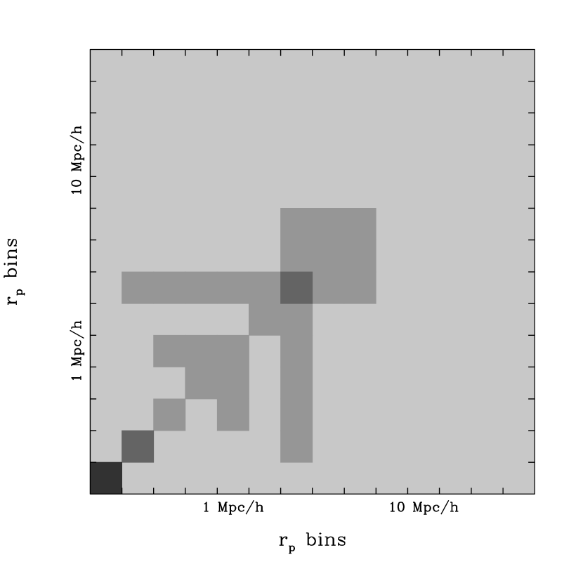
Figure A14: Jack-knife covariance matrix for the $M_{\mathrm{Pbar}}(r_{p})$ measurement of Fig. 7a. The grayscale as a function of galaxy separation indicates regions at which the measurement errors are correlated, such that darker regions have more correlated measurements.

Most of the errors are not strongly correlated, although the $r_{p}$ bins centered at 1 and $2\,\mathrm{Mpc}/h$ are weakly correlated with smaller-scale bins (most of which have stronger mark correlations), which may explain why the mark correlation measurements of these bins are slightly larger than in the neighboring $r_{p}$ bins.

In any case, the range of jack-knife clustering measurements in Figure A13 is not extremely large, and the correlations between the $r_{p}$ bins in Figure A14 are not extremely strong, so we conclude that the measured mark correlation functions are robust, as are the inferred environmental correlations.

References

- [Abazajian et al. (2009)] Abazajian K. N., et al., 2009, ApJS, 182, 543
- [Aguerri et al. (2009)] Aguerri J. A. L., Méndez-Abreu J., Corsini E. M., 2009, A&A, 495, 491
- [Athanassoula (2003)] Athanassoula E., 2003, MNRAS, 341, 1179
- [Bamford et al. (2009)] Bamford S. P., et al., 2009, MNRAS, 393, 1324
- [Barazza et al. (2008)] Barazza F. D., Jogee S., Marinova I., 2008, ApJ, 675, 1194
- [Barazza et al. (2009)] Barazza F. D., et al., 2009, A&A, 497, 713
- [Barway et al. (2011)] Barway S., Wadadekar Y., Kembhavi A. K., 2011, MNRAS, 410, L18
- [Baugh et al. (1996)] Baugh C. M., Cole S., Frenk C. S., 1996, MNRAS, 283, 1361
- [Beisbart & Kerscher (2000)] Beisbart C., Kerscher M., 2000, ApJ, 545, 6
- [Benson & Devereux (2010)] Benson A. J., Devereux N., 2010, MNRAS, 402, 2321
- [Berentzen et al. (2004)] Berentzen I., Athanassoula E., Heller C. H., Fricke K. J., 2004, MNRAS, 347, 220
- [Berentzen et al. (2007)] Berentzen I., Shlosman I., Martinez-Valpuesta I., Heller C. H., 2007, ApJ, 666, 189
- [Bernardi et al. (2010)] Bernardi M., Shankar F., Hyde J. B., Mei S., Marulli F., Sheth R. K., 2010, MNRAS, 404, 2087
- [Blanton et al. (2001)] Blanton M. R., et al., 2001, AJ, 121, 2358
- [Blanton et al. (2005)] Blanton M. R., Eisenstein D., Hogg D. W., Schlegel D. J., Brinkmann J., 2005, ApJ, 629, 143
- [Blanton & Roweis (2006)] Blanton M. R., Roweis S., 2007, AJ, 133, 734
- [Blanton & Berlind (2007)] Blanton M. R., Berlind A. A., 2007, ApJ, 664, 791
- [Bournaud & Combes (2002)] Bournaud F., Combes F., 2002, A&A, 392, 83
- [Bower et al. (2006)] Bower R. G., Benson A. J., Malbon R., Helly J. C., Frenk C. S., Baugh C. M., Cole S., Lacey C. G., 2006, MNRAS, 370, 645
- [Bruzual & Charlot (2003)] Bruzual G., Charlot S., 2003, MNRAS, 344, 1000
- [Bureau et al. (2006)] Bureau M., Aronica G., Athanassoula E., Dettmar R.-J., Bosma A., Freeman K., C., 2006, MNRAS, 370, 753
- [Buta et al. (2010)] Buta R., Laurikainen E., Salo H., Knapen J. H., 2010, ApJ, 721, 259
- [Cacciato et al. (2009)] Cacciato M., van den Bosch F. C., More S., Li R., Mo H. J., Yang X., 2009, MNRAS, 394, 929
- [Cameron et al. (2010)] Cameron E., et al., 2010, MNRAS, 409, 346
- [Chabrier (2003)] Chabrier G., 2003, ApJ, 586, L133
- [Cooper et al. (2010] Cooper M. C., Gallazzi A., Newman J. A., Yan R., 2010, MNRAS, 402, 1942
- [Cooray & Sheth (2002)] Cooray A., Sheth R., 2002, Phys. Rep., 372, 1
- [Croft et al. (2008)] Croft R. A. C., Di Matteo T., Springel V., Hernquist L., 2009, MNRAS, 400, 43
- [Dalcanton et al. (2004)] Dalcanton J. J., Yoachim P., Bernstein R. A., 2004, ApJ, 608, 189
- [Darg et al. (2010)] Darg D. W., et al., 2010, MNRAS, 401, 1043
- [Davé et al. (2011)] Davé R., Oppenheimer B. D., Finlator K., 2011, MNRAS, 415, 11
- [Debattista & Sellwood (2000)] Debattista V. P., Sellwood J. A.., 2000, ApJ, 543, 704
- [Debattista et al. (2006)] Debattista V. P., Mayer L., Carollo C. M., Moore B., Wadsley J., Quinn T., 2006, ApJ, 645, 209
- [de Lucia et al. (2011)] De Lucia G., Fontanot F., Wilman D., Monaco P., 2011, MNRAS, 414, 1439
- [de Vaucouleurs (1948)] de Vaucouleurs G., 1948, Ann. d’Astrophys., 11, 247
- [Dressler et al. (1980)] Dressler A., 1980, ApJ, 236, 351
- [Drory & Fisher (2007)] Drory N., Fisher D. B., 2007, ApJ, 664, 640
- [Ellison et al. (2010)] Ellison S. L., Patton D. R., Simard L., McConnachie A. W., Baldry I. K., Mendel J. T., 2010, MNRAS, 407, 1514
- [Ellison et al. (2011)] Ellison S. L., Nair P., Patton D. R., Scudder J. M., Mendel J. T., Simard L., 2011, MNRAS, 416, 2182
- [Elmegreen & Elmegreen (1985)] Elmegreen B. G., Elmegreen D. M., 1985, ApJ, 288, 438
- [Elmegreen et al. (1990)] Elmegreen D. M., Elmegreen B. G., Bellin A. D., 1990, ApJ, 364, 415
- [Elmegreen et al. (2011)] Elmegreen D. M., Elmegreen B. G., et al., 2011, ApJ, 737, 32
- [Emsellem et al. (2011)] Emsellem E., et al., 2011, MNRAS, 414, 888
- [Erwin (2005)] Erwin P., 2005, MNRAS, 364, 283
- [Fontanot et al. (2011)] Fontanot F., De Lucia G., Wilman D., Monaco P., 2011, MNRAS, 416, 409
- [Friedli et al. (1994)] Friedli D., Benz W., Kennicutt R., 1994, ApJ, 430, L105
- [Foyle et al. (2008)] Foyle K., Courteau S., Thacker R. J., 2008, MNRAS, 386, 1821
- [Gadotti (2009)] Gadotti D. A., 2009, MNRAS, 393 1531
- [Gadotti (2011)] Gadotti D. A., 2011, MNRAS, 415, 3308
- [Gardner, Connolly & McBride (2007)] Gardner J. P., Connolly A., McBride C., 2007, astro-ph/0709.1967
- [Giordano et al. (2011)] Giordano L., Tran K.-V., Moore B., Saintonge A., 2011, ApJ, submitted
- [Gottlöber et al. (2002)] Gottlöber S., Kerscher M., Kravtsov A. V., Faltenbacher A., Klypin A., Müller V., 2002, A&A, 387, 778
- [Graham (2011)] Graham A. W., 2011, in Keel W., ed., Planets, Stars and Stellar Systems, Vol. 6, Springer.
- [Guo et al. (2009)] Guo Y., et al., 2009, MNRAS, 398, 1129
- [Guo et al. (2011)] Guo H., Zehavi I., Zheng Z., 2011, ApJ, submitted
- [Haas, Schaye & Jeeson-Daniel (2011)] Haas M. R., Schaye J., Jeeson-Daniel A., 2012, MNRAS, 419, 2133
- [Hansen et al. (2008)] Hansen S. M., Sheldon E. S., Wechsler R. H., Koester B. P., 2009, ApJ, 699, 1333
- [Heller et al. (2007)] Heller C. H., Shlosman I., Athanassoula E., 2007, ApJ, 671, 226
- [Hopkins et al. (2009)] Hopkins P. F., et al., 2009, MNRAS, 397, 802
- [Hopkins et al. (2010)] Hopkins P. F., et al., 2010a, ApJ, 715, 202
- [Hopkins et al. (2010b)] Hopkins P. F., et al., 2010b, ApJ, 724, 915
- [Hopkins & Quataert (2010)] Hopkins P. F., Quataert E., 2010, MNRAS, 407, 1529
- [Hoyle et al. (2011)] Hoyle B., et al., 2011, MNRAS, 415, 3627
- [Jogee et al. (2005)] Jogee S. Scoville N., Kenney J. D. P., 2005, ApJ, 630, 837
- [Kauffmann et al. (2003)] Kauffmann G., et al., 2003, MNRAS, 341, 54
- [Kauffmann et al. (2004)] Kauffmann G., White S.D.M., Heckman T.M., Ménard B., Brinchmann J., Charlot S., Tremonti C., Brinkmann J., 2004, MNRAS, 353, 713
- [Kazantzidis et al. (2008)] Kazantzidis S., Bullock J. S., Zentner A. R., Kravtsov A. V., Moustakas L. A., 2008, ApJ, 688, 254
- [Keel et al. (1996)] Keel W. C., Byrd C. C., Klaric M., 1996, in Buta R., Crocker D. A., Elmegreen B. G., eds, Proc. IAU Colloq. 157, Barred Galaxies. Astron. Soc. Pac., San Francisco, p. 360
- [Kormendy & Kennicutt (2004)] Kormendy J., Kennicutt R. C., 2004, ARA&A, 42, 603
- [Kormendy & Bender (2011)] Kormendy J., Bender R., 2012, ApJS, 198, 2
- [Kuehn & Ryden (2005)] Kuehn F., Ryden B. S., 2005, ApJ, 634, 1032
- [Landy & Szalay (1993)] Landy S. D., Szalay A. S., 1993, ApJ, 412, 64
- [Larson et al. (1980)] Larson R. B., Tinsley B. M., Caldwell C. N., 1980, ApJ, 237, 692
- [Laurikainen et al. (2007)] Laurikainen E., Salo H., Buta R., Knapen J. H., 2007, MNRAS, 381, 401
- [Laurikainen et al. (2009)] Laurikainen E., Salo H., Buta R., Knapen J. H., 2009, ApJ, 692, L34
- [Lee et al. (2011)] Lee G.-H., Park C., Lee M. G., Choi Y.-Y., 2012a, ApJ, 745, 125
- [Lee et al. (2012)] Lee G.-H., Woo J.-H., Lee M. G., Hwang H. S., Lee J. C., Sohn J., Lee J. H., 2012b, ApJ, 750, 141
- [Li et al. (2009)] Li C., Gadotti D. A., Mao S., Kauffmann G., 2009, MNRAS, 397, 726
- [Li & White (2009)] Li C., White S. D. M., 2009, MNRAS, 398, 2177
- [Lintott et al. (2008)] Lintott C. J., et al., 2008, MNRAS, 389, 1179
- [Lintott et al. (2011)] Lintott C., et al., 2011, MNRAS, 410, 166
- [Lotz et al. (2011)] Lotz J. M., Jonsson P., Cox T. J., Croton D., Primack J. R., Somerville R. S., Stewart K., 2011, ApJ, 742, 103
- [Macciò et al. (2008)] Macciò A. V., Dutton A. A., van den Bosch F. C., 2008, MNRAS, 391, 1940
- [Madgwick et al. (2003)] Madgwick D. S., et al., 2003, MNRAS, 344, 847
- [Mandelbaum et al. (2009)] Mandelbaum R., Li C., Kauffmann G., White S. D. M., 2009, MNRAS, 393, 377
- [Maraston (2005)] Maraston C., 2005, MNRAS, 362, 799
- [Marinova et al. (2009)] Marinova I., et al., 2009, ApJ, 698, 1639
- [Marinova et al. (2012)] Marinova I., et al., 2012, ApJ, 746, 136
- [Martig et al. (2012)] Martig M., Bournaud F., Croton D. J., Dekel A., Teyssier R., 2012, ApJ, submitted
- [Martinez et al. (2010)] Martínez V. J., Arnalte-Mur P., Stoyan D., 2010, A&A, 513, 22
- [Martinez & Muriel (2011)] Martínez H. J., Muriel H., 2011, MNRAS, 418, L148
- [Masters et al. (2010)] Masters K. L., et al., 2010a, MNRAS, 404, 792
- [Masters et al. (2010b)] Masters K. L., et al., 2010b, MNRAS, 405, 783
- [Masters et al. (2011)] Masters K. L., et al., 2011, MNRAS, 411, 2026 (M11)
- [Masters et al. (2012)] Masters K. L., et al., 2012, MNRAS, in press (arXiv:1205.5271))
- [McBride et al. (2011)] McBride C. K., Connolly A. J., Gardner J. P., Scranton R., Newman J. A., Scoccimarro R., Zehavi I., Schneider D. P., 2011, ApJ, 726, 13
- [McKernan et al. (2010)] McKernan B., Ford K. E. S., Reynolds C. S., 2010, MNRAS, 407, 2399
- [Mendez-Abreu et al. (2010)] Méndez-Abreu J., Sánchez-Janssen R., Aguerri J. A. L., 2010, ApJ, 711, L61
- [Menendez-Delmestre et al. (2007)] Menéndez-Delmestre K., Sheth K., Schinnerer E., Jarrett T. H., Scoville N. Z., 2007, ApJ, 657, 790
- [Miwa & Noguchi (1998)] Miwa T., Noguchi M., 1998, ApJ, 499, 149
- [More et al. (2009)] More S., van den Bosch F., Cacciato M., Mo H.J., Yang X., Li R., 2009, MNRAS, 392, 801
- [Muldrew et al. (2011)] Muldrew S. I., Croton D. J., Skibba R. A., Pearce F. R., et al., 2012, MNRAS, 419, 2670
- [Nair & Abraham (2010)] Nair P. B., Abraham R. G., 2010, ApJ, 714, L260
- [Navarro et al. (1996)] Navarro J. F., Frenk C. S., White S. D. M., 1996, ApJ, 462, 563
- [Noguchi (1996)] Noguchi M., 1996, ApJ, 469, 605
- [Norberg et al. (2008)] Norberg P., Baugh C. M., Gaztañaga E., Croton D. J., 2009, MNRAS, 396, 19
- [Norberg et al. (2011)] Norberg P., Gaztañaga E., Baugh C. M., Croton D. J., 2011, MNRAS, 418, 2435
- [O’Neill & Dubinski (2003)] O’Neill J. K., Dubinski J., 2003, MNRAS, 346, 251
- [Park et al. (2007)] Park C., Choi Y.-Y., Vogeley M. S., Gott III J. R., Blanton M. R., 2007, ApJ, 658, 898
- [Parry et al. (2009)] Parry O. H., Eke V. R., Frenk C. S., 2009, MNRAS, 396, 1972
- [Pasquali et al. (2009)] Pasquali A., van den Bosch F. C., Mo H.J., Yang X., Somerville R., 2009, MNRAS, 394, 38
- [Perez & Sanchez-Blazquez (2011)] Pérez I., Sánchez-Blázquez P., 2011, A&A, 529, A64
- [Postman & Geller (1984)] Postman M., Geller M. J., 1984, ApJ, 281, 95
- [Romano-Diaz et al. (2008)] Romano-Díaz E., Shlosman I., Heller C., Hoffman Y., 2008, ApJ, 687, L13
- [Sales et al. (2011)] Sales L. V., Navarro J. F., Theuns T., Schaye J., White S. D. M., Frenk C. S., Crain R. A., Dalla Vecchia C., 2012, MNRAS, 423, 1544
- [Sanchez-Blazquez et al. (2011)] Sánchez-Blázquez P., Ocvirk P., Gibson B. K., Pérez I., Peletier R. F., 2011, MNRAS, 415, 709
- [Scannapieco et al. (2010)] Scannapieco C., Gadotti D. A., Jonsson P., White S. D. M., 2010, MNRAS, 407, L41
- [Schawinski et al. (2010)] Schawinski K., et al., 2010, ApJ, 711, 284
- [Schiminovich et al. (2007)] Schiminovich D., et al., 2007, ApJS, 173, 315
- [Schlegel et al. (1998)] Schlegel D. J., Finkbeiner D. P., Davis M., 1998, ApJ, 500, 525
- [Scranton et al. (2005)] Scranton R. et al., 2005, ApJ, 633, 589
- [Sellwood & Wilkinson (1993)] Sellwood J. A., Wilkinson A., 1993, Rep. Prog. Phys., 56, 173
- [Sheldon et al. (2007)] Sheldon E. S., et al., 2009, ApJ, 703, 2217.
- [Sheth et al. (2005)] Sheth K., et al., 2005, ApJ, 632, 217
- [Sheth et al. (2008)] Sheth K., et al., 2008, ApJ, 675, 1141
- [Sheth, Connolly & Skibba 2005 (2005)] Sheth R. K., Connolly A. J., Skibba R., 2005, astro-ph/0511773
- [Sheth et al. (2006)] Sheth R. K., Jimenez R., Panter B., Heavens A. F., 2006, ApJ, 650, L25
- [Skibba et al. (2006)] Skibba R. A., Sheth R. K., Connolly A. J., Scranton R., 2006, MNRAS, 369, 68
- [Skibba & Sheth (2009)] Skibba R. A., Sheth R. K., 2009, MNRAS, 392, 1080
- [Skibba (2009)] Skibba R. A., 2009, MNRAS, 392, 1467
- [Skibba et al. (2009)] Skibba R. A., Bamford S. P., Nichol R. C., et al., 2009, MNRAS, 399, 966 (S09)
- [Springel et al. (2005)] Springel V., et al., 2005, Nature, 435, 629
- [Stoyan & Stoyan (1994)] Stoyan D., Stoyan H., 1994, Fractals, Random Shapes, and Point Fields. Wiley, Chichester
- [Strateva et al. (2001)] Strateva I., et al., 2001, AJ, 122, 1861
- [Strauss et al. (2002)] Strauss M. A., et al., 2002, AJ, 124, 1810
- [Subbarao et al. (2002)] Subbarao M., Frieman J., Bernardi M., Loveday J., Nichol B., Castander F., Meiksin A., 2002, SPIE, 4847, 452
- [Tinker et al. (2008)] Tinker J. L., Conroy C., Norberg P., Patiri S. G., Weinberg D. H., Warren M. S., 2008, ApJ, 686, 53
- [Valenzuela & Klypin (2003)] Valenzuela O., Klypin A., 2003, MNRAS, 345, 406
- [van den Bergh (2002)] van den Bergh S., 2002, AJ, 124, 782
- [van der Wel (2008)] van der Wel A., 2008, ApJ, 675, L13
- [van der Wel (2010)] van der Wel A., Bell E. F., Holden B. P., Skibba R. A., Rix H.-W., 2010, ApJ, 714, 1779
- [Vincent & Ryden (2005)] Vincent R. A., Ryden B. S., 2005, ApJ, 623, 137
- [Weinberg & Katz (2002)] Weinberg M. D., Katz N., 2002, ApJ, 580, 627
- [Weinberg & Katz (2007)] Weinberg M. D., Katz N., 2007, MNRAS, 375, 460
- [Weinzirl et al. (2009)] Weinzirl T., Jogee S., Khochfar S., Burkert A., Kormendy J., 2009, ApJ, 696, 411
- [Wetzel et al. (2007)] Wetzel A. R., Cohn J. D., White M., Holz D. E., Warren M. S., 2007, ApJ, 656, 139
- [White & Padmanabhan (2009)] White M., Padmanabhan N., 2009, MNRAS, 395, 2381
- [Wilman et al. (2010)] Wilman D. J., Zibetti S., Budavári T., 2010, MNRAS, 406, 1701
- [Wilman & Erwin (2011)] Wilman D. J., Erwin P., 2012, ApJ, 746, 160
- [Wyder et al. (2007)] Wyder T. K., et al., 2007, ApJS, 173, 293
- [York et al. (2000)] York D. G. et al., 2000, AJ, 120, 1579
- [Zehavi et al. (2004)] Zehavi I., et al., 2004, ApJ, 608, 16
- [Zehavi et al. (2005)] Zehavi I., et al., 2005, ApJ, 630, 1
- [Zehavi et al. (2011)] Zehavi I., et al., 2011, ApJ, 736, 59
- [Zheng et al. (2007)] Zheng Z., Coil A. L., Zehavi I., 2007, ApJ, 667, 760
- [Zibetti et al. (2009)] Zibetti S., Charlot S., Rix H.-W., 2009, MNRAS, 400, 1181