Recovering Model Structures from Large Low Rank and Sparse Covariance Matrix Estimation

Abstract

Abstract. Many popular statistical models, such as factor and random effects models, give arise a certain type of covariance structures that is a summation of low rank and sparse matrices. This paper introduces a penalized approximation framework to recover such model structures from large covariance matrix estimation. We propose an estimator based on minimizing a non-likelihood loss with separable non-smooth penalty functions. This estimator is shown to recover exactly the rank and sparsity patterns of these two components, and thus partially recovers the model structures. Convergence rates under various matrix norms are also presented. To compute this estimator, we further develop a first-order iterative algorithm to solve a convex optimization problem that contains separable non-smooth functions, and the algorithm is shown to produce a solution within $O(t^{-2})$ of the optimal, after any finite $t$ iterations. Numerical performance is illustrated using simulated data and stock portfolio selection on S&P 100.

Keywords: model recovery, factor model, Nesterov’s algorithm, lasso, nuclear norm, portfolio selection.

1 Introduction

Covariance estimation is important in multivariate modeling. The natural estimator, sample covariance, is known to perform badly in high dimensions, where the number of variables is larger than or comparable to the sample size. Various structural assumptions have been imposed to stabilize this estimator. However, recovering the statistical models that lead to such structural assumptions is under explored. As a matter of fact, popular statistical models, such as random effects and factor models, entail a new type of covariance structures than studied before. In this paper, we propose a unified approach to recover the covariance structures and the model structures from large dimensional data.

To begin with, suppose we observe $\mathbf{X}_{1},\dotsc,\mathbf{X}_{n}\in\mathbb{R}^{p}$ iid from a multivariate Gaussian distribution $N(\mu,\mathbf{\mathbf{\mathbf{\Sigma}}}^{*})$. The canonical estimator for $\mathbf{\Sigma}^{*}$ is the sample covariance

$$\mathbf{\Sigma}_{n}=\frac{1}{n-1}\sum_{i=1}^{n}(\mathbf{X}_{i}-\bar{\mathbf{X}})(\mathbf{X}_{i}-\bar{\mathbf{X}})^{T}$$

where the sample mean $\bar{\mathbf{X}}=(1/n)\sum_{i=1}^{n}\mathbf{X}_{i}$. Figure 1 illustrates the sample covariance and correlation matrices of 53 monthly stock returns from year 1972-2009. Details about this dataset can be found in Section 5.2. Note that 86.14% of the correlation entries are larger than 0.2, more than 50% are larger than 0.3.

Figure 1: Sample covariance and correlation of monthly returns of SP100 from 1972-2009.

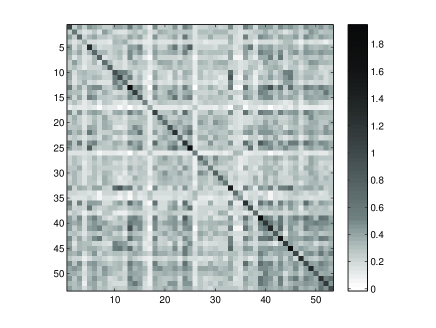
(a) Sample Covariance

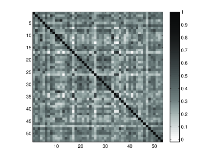
(b) Sample Correlation

Regularizing $\mathbf{\Sigma}_{n}$ was proposed in the literature to stabilize the estimator, mostly aiming for studying matrix norm losses under different structural assumptions. In the time series setting, Bickel and Levina (2008a) proposed banding $\mathbf{\Sigma}_{n}$, and the optimal convergence rate was established in Cai et al. (2010b). Wu and Pourahmadi (2003); Huang et al. (2006) employed regularized regression on modified Cholesky factors. In a setting where the indexing order is unavailable, thresholding $\mathbf{\Sigma}_{n}$ was proposed by Bickel and Levina (2008b). Generalized thresholding rules were considered in Rothman et al. (2009), and an adaptive thresholding rule was proposed by Cai and Liu (2011). There and in what follows, sparsity means the number of nonzero off-diagonal entries is small comparing to the sample size. Without imposing such explicit structural assumptions, shrinkage estimation was proposed by Ledoit and Wolf (2004). This paper also studies the order invariant situation, but aims to recover the model structures from covariance estimation. First of all, it seems to be unnatural to apply thresholding directly for our dataset in Figure 1, partly because most of the entries have large magnitude. On the other hand, factor models have been widely used for modeling stock data (Sharpe, 1964; Fama and French, 1992), and for estimating the non-sparse covariance matrix (Fan et al., 2008). To this end, we introduce a decomposition framework to recover a general form of covariance structures, which includes hidden factor models as a special case.

This paper proposes a unified framework that entails the following covariance structure

$$\mathbf{\mathbf{\Sigma}}^{*}=\mathbf{L}^{*}+\mathbf{S}^{*}$$ (1)

where $\mathbf{L}^{*}$ is a low rank component and $\mathbf{S}^{*}$ is a sparse component. This framework is motivated by several important statistical models. A few examples are outlined below.

1. Factor analysis: consider the following concrete model

   $$\mathbf{X}=\mathbf{B}\mathbf{f}+\mathbf{\epsilon}$$ (2)

   where $\mathbf{B}$ is a fixed matrix in $\mathbb{R}^{p\times K}$, factor $\mathbf{f}\in\mathbb{R}^{K}$ and error $\mathbf{\epsilon}\in\mathbb{R}^{p}$ are independently generated from random processes. Factor model (2) was widely studied in statistics (Anderson, 1984), in genetics (Leek and Storey, 2007), in economics and finance (Ross, 1976; Chamberlain and Rothschild, 1983; Fama and French, 1992), and in signal processing (Krim and Viberg, 1996). The number of factors, $K$, is usually assumed to be small, for example, $K=1$ in the capital asset pricing model (CAPM) (Sharpe, 1964) and $K=3$ in the Fama-French model (Fama and French, 1992). It is easy to see that the implied covariance matrix of model (2) is

   $$\mathbf{\Sigma}^{*}=\mathbf{B}\operatorname{Var}(\mathbf{f})\mathbf{B}^{T}+\mathbf{\Sigma}_{\mathbf{\epsilon}}$$ (3)

   where the error covariance $\mathbf{\Sigma}_{\mathbf{\epsilon}}=\mathbb{E}\mathbf{\epsilon}\mathbf{\epsilon}^{T}.$ Note that $\mathbf{B}\operatorname{Var}(\mathbf{f})\mathbf{B}^{T}$ has at most rank $K$. Linear regression approach under (3) was proposed by Fan et al. (2008), assuming that $\mathbf{f}$ is observable (thus $K$ is known) and $\mathbf{\Sigma}_{\mathbf{\epsilon}}$ is diagonal. This paper instead studies a hidden $\mathbf{f}$ setting, and we will assume a more general assumption that $\mathbf{\Sigma}_{\mathbf{\epsilon}}$ is sparse in the spirit of Bickel and Levina (2008b). This more general assumption is particularly useful in modeling stock data (Chamberlain and Rothschild, 1983). Our method recovers both the rank $K$ and the non-zero entries in $\mathbf{\Sigma}_{\mathbf{\epsilon}}$. An improved convergence rate $O(n^{-1/2}(p+p^{1/2}K^{1/2})$ is also established under the Frobenius norm, comparing with the rate $O(n^{-1/2}pK)$ in Fan et al. (2008). These results serve as an important step towards adapting to the order $K$ of hidden factor models and modeling possible correlated errors.

2. Random effects: take the Compound Symmetry model below as an illustrating case

   $$\mathbf{\Sigma}^{*}=\sigma_{b}^{2}\mathbf{1}^{T}\mathbf{1}+\mathbf{S}^{*}$$ (4)

   where $\sigma_{b}^{2}$ and $\mathbf{S}^{*}$ are between-subject and within-subject variances respectively. More examples with two component decompositions similar to (4) can be found a standard textbook (Fitzmaurice et al., 2004). General non-diagonal $\mathbf{S}^{*}$ was studied by Jennrich and Schluchter (1986), but only for an AR(1) type. We aim to recover sparse $\mathbf{S}^{*}$ as well as the fist rank 1 component in (4).

3. Spiked covariance: Johnstone and Lu (2009) proposed a spiked covariance model

   $$\mathbf{\Sigma}^{*}=\beta\mathbf{u}\mathbf{u}^{T}+\mathbf{S}^{*}$$ (5)

   where most of the coordinates of $\mathbf{u}$ are zero. Under the assumption $\mathbf{S}^{*}=\sigma^{2}\mathbf{I}$, they proved inconsistency results for $\mathbf{u}$ using classical PCA, and proposed a consistent approach called sparse PCA. Amini and Wainwright (2009) established consistent subset selection on the nonzero coordinates of $\mathbf{u}$, under the scaling $n\geq Ck^{2}\log(p-k)$, where $k$ is the number of the nonzero components in $\mathbf{u}$. Our estimator (with a simple modification) achieves the same scaling but continues to hold for sparse and non-diagonal $\mathbf{S}^{*}$.

4. Conditional covariance: following Anderson (1984), suppose a multivariate normal vector $\mathbf{X}=(\mathbf{X}_{1}^{T},\mathbf{X}_{2}^{T})^{T}$, conditioning on the subvector $\mathbf{X}_{2}$, the conditional covariance of the subvector $\mathbf{X}_{1}$ is

   $$\mathbf{\Sigma}^{*}=-\mathbf{\Sigma}_{12}\mathbf{\Sigma}_{22}^{-1}\mathbf{\Sigma}_{21}+\mathbf{\Sigma}_{11}$$

   where $\mathbf{\Sigma}_{ij}$, for $i,j=1,2$, is standard matrix partition of the full covariance. The first component have rank upper bounded by the length of $\mathbf{X}_{2}$, and the marginal covariance $\mathbf{\Sigma}_{11}$ is assumed to be sparse. Model based approaches have been heavily explored in the finance literature. Our method provides an alternative approach that is non-model based and with statistical performance guarantees.

In summary, our general framework (1) recovers the model structures from several statistical models. Of course, the list of models is no way complete.

To exploit the low rank and sparse structures in (1), we propose a non-likelihood approximation criterion with a composite penalty, called LOw Rank and sparsE Covariance estimator (LOREC). Methods based on non-likelihood criteria were proposed by several investigators before (Yuan, 2010; Cai et al., 2011; Agarwal et al., 2011; Liu and Luo, 2012). Specifically, this paper employs a Frobenius norm approximation criterion because it enjoys several advantages in computation and theoretical analysis. To exploit the low rank and sparse components in (1), we adopt a composite penalty combining the nuclear norm (Fazel et al., 2001) and the $\ell_{1}$ norm (Tibshirani, 1996). The same type of composite penalty was employed under different settings before (Candes et al., 2009; Chandrasekaran et al., 2010). We extend their analysis ideas to establish the theoretical guarantees of LOREC. Because the problems are different, LOREC achieves improved convergence rates under a relaxed sample size requirement, see Section 3.

After this work was posted and submitted, a reviewer suggested a recent work by Agarwal et al. (2011). There are a few major differences. First, they studied a nearly low-rank setting comparing with our exact low rank setting. Moreover, They aimed to establish the minimax optimality under the joint squared Frobenius norm loss

$$e^{2}\left(\hat{\mathbf{L}},\hat{\mathbf{S}}\right):=\left|\hat{\mathbf{L}}-\mathbf{L}^{*}\right|_{F}^{2}+\left|\hat{\mathbf{S}}-\mathbf{S}^{*}\right|_{F}^{2}$$ (6)

where $\hat{\mathbf{L}}$ and $\hat{\mathbf{S}}$ are the estimators for $\mathbf{L}^{*}$ and $\mathbf{S}^{*}$ respectively. In comparison, LOREC aims to recover model structures via the operator and max norm bounds

$$\left\|\hat{\mathbf{L}}-\mathbf{L}^{*}\right\|_{2}\quad\mbox{and}\quad\left|\hat{\mathbf{S}}-\mathbf{S}^{*}\right|_{\infty}.$$ (7)

In Section 2, we further outline several major differences between two approaches. The structure recovery performance is further compared and illustrated by both simulated data and a real data example in Section 5. Finally, this paper provides additional algorithmic advantages which we now turn to.

To efficiently compute for large scale problems, we further develop Nesterov’s method (Nesterov, 1983; Nesterov and Nesterov, 2004) to a general composite penalization setting when two non-smooth functions are separable. We extends the complexity analysis by Ji and Ye (2009) to this general setting. Our algorithm is shown to achieve an iteration complexity of $O(t^{-2})$, after any finite $t$ iterations. In comparison, the finite complexity analysis was unfortunately unavailable in Chandrasekaran et al. (2010) and Agarwal et al. (2011), possibly due to the complex numerical projections employed by their methods and algorithms. To our best knowledge, LOREC is the first computationally trackable and publicly available algorithm for recovering model structures from low rank and sparse covariance matrix decompositions.

This paper is organized as follows. In Section 2, we introduce our problem set up and our method based on convex optimization. Its statistical loss bounds are presented in Section 3. Our algorithmic developments are discussed in Section 4, and its complexity analysis is also discussed. The numerical performance is illustrated in Section 5, by both simulation examples and a real data set. Possible future directions are discussed in Section 6. Implications of the results and all proofs are included in the supplementary materials online. All convergence and complexity results are non-asymptotic.

Notations Let $\mathbf{M}=(M_{ij})$ be any matrix. The following matrix norms on $\mathbf{M}$ will be used: $\lvert\mathbf{M}\rvert_{1}=\sum_{i}\sum_{j}\lvert M_{ij}\rvert$ stands for the elementwise $\ell_{1}$ norm; $\left\|\mathbf{M}\right\|_{1}=\max_{j}\sum_{i}\left|M_{ij}\right|$ for the matrix $\ell_{1}$ norm; $\lvert\mathbf{M}\rvert_{\infty}=\max_{i,j}\lvert M_{ij}\rvert$ for the elementwise $\ell_{\infty}$ norm or the max norm; $\lvert\mathbf{M}\rvert_{F}=\sqrt{\sum_{i}\sum_{j}M_{ij}^{2}}$ for the Frobenius norm; $\lVert\mathbf{M}\rVert_{*}=\sum_{i}D_{ii}$ for the nuclear (trace) norm if the SVD decomposition $\mathbf{M}=\mathbf{U}\mathbf{D}\mathbf{V}^{T}$. We denote $\langle\mathbf{A},\mathbf{B}\rangle:=\operatorname{trace}(\mathbf{A}^{T}\mathbf{B})$ for matrices $\mathbf{A}$ and $\mathbf{B}$ of proper sizes. We also denote the vectorization of a matrix $M$ by $\operatorname{vec}(M)$. The identity matrix is denoted by $\mathbf{I}$, and the vector of all ones is denoted by $\mathbf{1}$. Generic constants are denoted by $C,C_{1},C_{2},\dotsc$, and they may represent different values at each appearance.

2 Method

We introduce the LOREC estimator in this section. Existing approaches that motivate LOREC will be briefly reviewed first. Other variants and extensions of LOREC will discussed in Section 6.

Given a sample covariance matrix $\mathbf{\Sigma}_{n}$, low rank approximation seeks a matrix $\mathbf{M}$ that is equivalent to optimize

$$\min_{\mathbf{M}}\left\{\frac{1}{2}\left|\mathbf{M}-\mathbf{\Sigma}_{n}\right|_{F}^{2}+\lambda\operatorname{rank}(\mathbf{M})\right\}$$ (8)

for some penalization parameter $\lambda>0$. The multiplier $1/2$ before the Frobenius norm is not essential, and is chosen here for simplicity in analysis. This estimator is known as low rank approximation in matrix computation (Horn and Johnson, 1994). Recently, this rank penalty was also studied in the regression setting (Bunea et al., 2011). Unfortunately, its connection to model recovery was unclear, and the resulting estimator from (8) is rank deficient and thus not appropriate for estimating a full rank $\mathbf{\Sigma}^{*}$.

Recently, Bickel and Levina (2008b) proposed an elementwise thresholding method. It is equivalent to the following optimization

$$\min_{\mathbf{M}}\left\{\frac{1}{2}\left|\mathbf{M}-\mathbf{\mathbf{\Sigma}}_{n}\right|_{F}^{2}+\sum_{i,j}\mathrm{pen}_{\rho}(M_{ij})\right\}$$ (9)

where the hard thresholding penalty is $2\mathrm{pen}_{\rho}(x)=\rho^{2}-(\left|x\right|-\rho)^{2}1\left\{\left|x\right|<\rho\right\}$ for some thresholding level $\rho>0$. Other penalty forms were studied in Rothman et al. (2009). The underlying sparsity assumption in this approach is not immediately clear under some classical multivariate models, as illustrated in Section 1. Therefore, thresholding provides limited model recovery. More importantly, many data examples suggest a non-sparse covariance structure, as in Figure 1.

To address these concerns, we let $\mathbf{\Sigma}^{*}$ to be a low rank matrix plus a sparse matrix in (1). A sparse component (possibly positive definite) overcomes the rank deficiency of low rank approximation, and a low rank component enables model recovery under a few statistical models discussed in Section 1. Under the decomposition (1), it is natural to consider a two-component estimator $\hat{\mathbf{\Sigma}}=\hat{\mathbf{L}}+\hat{\mathbf{S}}$, with a low rank matrix $\hat{\mathbf{L}}$ and a sparse matrix $\hat{\mathbf{S}}$. To enforce such properties, one may combine the two penalty functions from (8) and (9) in the following objective function

$$\min_{\mathbf{L},\mathbf{S}}\left\{\frac{1}{2}\left|\mathbf{L}+\mathbf{S}-\mathbf{\Sigma}_{n}\right|_{F}^{2}+\lambda\operatorname{rank}(\mathbf{L})+\sum_{i,j}\mathrm{pen}_{\rho}(S_{ij})\right\}.$$ (10)

However, the objective function (10) is computationally intractable, because this is a combinatorial optimization problem in general. We replace the penalty functions with their computationally efficient counterparts: the $\ell_{1}$ norm heuristic (Tibshirani, 1996; Friedman et al., 2008), and the nuclear norm regularization (Fazel et al., 2001). We thus propose the LOREC estimator $\hat{\mathbf{\Sigma}}=\mathbf{\hat{L}}+\hat{\mathbf{S}}$ that derives from the following optimization

$$\min_{\mathbf{L},\mathbf{S}}\left\{\frac{1}{2}\left|\mathbf{L}+\mathbf{S}-\mathbf{\Sigma}_{n}\right|_{F}^{2}+\lambda\lVert\mathbf{L}\rVert_{*}+\rho\lvert\mathbf{S}\rvert_{1}\right\}$$ (11)

where $\lambda>0$ and $\rho>0$ are two penalization parameters. This objective is convex and can be solved efficiently. In Section 4, we further develop Nesterov’s algorithm to this composite penalty setting. An important observation is that the non-smooth penalty functions are separable in iterative updates, and thus each update can be expressed in closed form. Complexity bounds (Ji and Ye, 2009) are further extended to this general setting as well. Note that the symmetry of $\left(\mathbf{L},\mathbf{S}\right)$ is always guaranteed because the objective is invariant under transposition.

The Frobenius norm loss in (11) deserves some remarks. First, it is a natural extension of the mean squared loss for vectors. Indeed it is the $\ell_{2}$ norm of either eigenvalues or matrix entries, and thus it is a natural distance for both low rank and sparse matrix spaces. The second reason is that it provides a model-free method, as covariance is also model-free. Even if a likelihood function exists, there are some advantages of employing such non-likelihood methods, see Meinshausen and Bühlmann (2006); Cai et al. (2011) for example. Finally, the Frobenius norm loss enables fast computation.

There are several variants under this framework. The sample covariance $\mathbf{\Sigma}_{n}$ in (11) can be replaced by any other reasonable estimator close to the underlying covariance. For example, we illustrate in Section 3.3 by replacing with a thresholded sample covariance. Furthermore, other penalties can be used in (11) instead. For example, the diagonal can be unpenalized by the off-diagonal $\ell_{1}$ norm defined as $\lvert S\rvert_{1,o}=\sum_{i\neq j}\lvert S_{ij}\rvert$. Other possible choices will be discussed in Section 6. To fix ideas, we will stick to the formulation (11) for the rest of the paper.

After this paper was posted and submitted, a review suggested a recent work by Agarwal et al. (2011), hereafter ANW. ANW studied theoretical aspects using a joint loss (6) and employed a further constrained objective function, extending (11). In our notation, their proposal can be written as

$$\min_{\mathbf{L},\mathbf{S}}\left\{\frac{1}{2}\left|\mathbf{L}+\mathbf{S}-\mathbf{\Sigma}_{n}\right|_{F}^{2}+\lambda\lVert\mathbf{L}\rVert_{*}+\rho\lvert\mathbf{S}\rvert_{1}\right\}\quad\mbox{such that}\,\left|\mathbf{L}\right|_{\infty}\leq\frac{\alpha}{p}$$ (12)

where $\alpha>0$ is a third tuning parameter. Intuitively, the added constraint on $\mathbf{L}$ introduces biases towards matrices that are not only low rank but also have small entries, which unfortunately is not well motivated by the statistical models discussed before. In addition to the added complication in ANW, there are several other major differences between ANW and LOREC, from the theoretical, computational, and numerical prospectives. Firstly, ANW aimed to address nearly low-rank matrix decompositions, and the low rank component may be biased under the additional max norm constraint. LOREC, on the other hand, recovers exactly low rank and sparse matrices under separate losses (7). This separate recovery enables recovering model structures, see Section 3. As we will also show using extensive numerical examples in Section 5, ANW, unfortunately, may not recover model structures while LOREC does, as predicted by the analysis. Secondly, the Frobenius norm bounds in ANW can be derived from the separate bounds (7) for LOREC because our bounds are stronger, though we don’t establish minimax optimality in this paper. We further argue that the joint loss by ANW provided limited performance guarantees in many important applications. For example, LOREC provides such guarantees for $\left(\mathbf{L}^{*}+\mathbf{S}^{*}\right)^{-1}$ under the spectral norm, which is essential for portfolio selection on a real data example in Section 5.2. Thirdly, optimal covariance estimators under the Frobenius loss were shown to be different from the optimal ones under the spectral norm (Cai et al., 2010b). Finally, it is unclear how the ANW estimator can be computed efficiently with finite iteration complexity bounds, while we establish this property in Section 4. To our best knowledge, LOREC is the first computationally tractable approach for recovering model structures via performing covariance matrix decomposition.

3 Theoretical Guarantees

We show our main results regarding the theoretical performance of LOREC first, without assuming any specific model structure. We then discuss the implications under the spiked covariance model, and compare with existing results. Implications under other models can be found in the supplemental materials online.

3.1 Results for Recovering General Matrix Structures

For the identifiability of $\mathbf{L}^{*}$ and $\mathbf{S}^{*}$, we need some additional assumptions. These assumptions were proposed by Candes et al. (2009); Chandrasekaran et al. (2010). The following definitions are needed for the analysis. For any matrix $\mathbf{M}\in\mathbb{R}^{p\times p}$, define the following tangent spaces

$$\Omega(\mathbf{M}) =\left\{\mathbf{N}\in\mathbb{R}^{p\times p}\,|\,\operatorname{support}(\mathbf{N})\subseteq\operatorname{support}(\mathbf{M})\right\},$$

$$T(\mathbf{M}) =\left\{\mathbf{U}\mathbf{Y}_{1}^{T}+\mathbf{Y}_{2}\mathbf{V}^{T}\,|\,\mathbf{Y}_{1},\mathbf{Y}_{2}\in\mathbb{R}^{p\times r}\right\}$$

where the SVD decomposition $\mathbf{M}=\mathbf{U}\mathbf{D}\mathbf{V}^{T}$ with $\mathbf{U}\in\mathbb{R}^{p\times r}$, $\mathbf{V}\in\mathbb{R}^{p\times r}$ and diagonal $\mathbf{D}\in\mathbb{R}^{r\times r}$. In addition, define the measures of coherence between $\Omega(\mathbf{M})$ and $T(\mathbf{M})$ by

$$\xi(T(\mathbf{M})) =\max_{\mathbf{N}\in T(\mathbf{M}),\,\left\|\mathbf{N}\right\|_{2}\leq 1}\left|\mathbf{N}\right|_{\infty,}$$

$$\mu(\Omega(\mathbf{M})) =\max_{\mathbf{N}\in\Omega(\mathbf{M}),\,\left|\mathbf{N}\right|_{\infty}\leq 1}\left\|\mathbf{N}\right\|_{2}.$$

Detailed discussions of the above quantities $\Omega(\mathbf{M})$, $T(\mathbf{M})$, $\xi(T(\mathbf{M}))$ and $\mu(\Omega(\mathbf{M}))$ and their implications can be found in Chandrasekaran et al. (2010). We will give an explicit form of these quantities under the spiked model, see Section 3.3.

To characterize the convergence of $\mathbf{\Sigma}_{n}$ to $\mathbf{\Sigma}^{*}$, we assume $\mathbf{\Sigma}^{*}$ to be within the following matrix class

$$\mathcal{U}(\epsilon_{0})=\left\{\mathbf{M}\in\mathbb{R}^{p\times p}:\,0<\epsilon_{0}\leq\Lambda_{i}(\mathbf{M})\leq\epsilon_{0}^{-1}<+\infty,\,\mathrm{for}\,i=1,\dotsc,p\right\}$$

where $\Lambda_{i}(\mathbf{M})$ denotes the $i$th largest singular value of $\mathbf{M}$. The largest eigenvalue of $\mathbf{\Sigma}^{*}$ is then $\Lambda_{\max}:=\Lambda_{1}(\mathbf{\Sigma}^{*})$, and the smallest is $\Lambda_{\min}:=\Lambda_{p}(\mathbf{\Sigma}^{*})$. Similar covariance classes (with additional constraints) were considered in the bandable setting (Bickel and Levina, 2008a; Cai et al., 2010b) and in the sparse setting (Bickel and Levina, 2008b; Cai et al., 2011; Cai and Liu, 2011).

We have the following general theorem on the statistical performance of LOREC.

Theorem 1.

Let $\Omega=\Omega(\mathbf{S}^{*})$ and $T=T(\mathbf{L}^{*})$. Suppose that $\mathbf{\Sigma}^{*}\in\mathcal{U}(\epsilon_{0})$, $\mu(\Omega)\xi(T)\leq 1/54$, and for $n\geq p$ that

$$\lambda=C_{1}\max\left(\frac{1}{\xi(T)}\sqrt{\frac{\log p}{n}},\sqrt{\frac{p}{n}}\right)$$

and $\rho=\gamma\lambda$ where $\gamma\in\left[9\xi(T),1/(6\mu(\Omega))\right].$ In addition, suppose the minimal singular value of $\boldsymbol{L}^{*}$ is greater than $C_{2}\lambda/\xi^{2}(T)$, and the smallest absolute value of the nonzero entries of $\mathbf{S}^{*}$ is greater than $C_{3}\lambda/\mu(\Omega)$. Then with probability greater than $1-C_{4}p^{-C_{5}}$, the LOREC estimator $(\hat{\mathbf{L}},\hat{\mathbf{S}})$ recovers the rank of $\mathbf{L}^{*}$ and the sparsity pattern of $\mathbf{S}^{*}$ exactly, that is

$$\operatorname{rank}(\mathbf{\hat{L}})=\operatorname{rank}(\mathbf{L}^{*})\quad\textrm{and}\quad\operatorname{sign}(\hat{\mathbf{S}})=\operatorname{sign}(\mathbf{S}^{*}).$$

Moreover, with probability greater than $1-C_{4}p^{-C_{5}}$, the matrix losses for each component are bounded as follows

$$\left\|\hat{\mathbf{L}}-\mathbf{L}^{*}\right\|_{2}\leq C\lambda\quad\textrm{and}\quad\left|\hat{\mathbf{S}}-\mathbf{S}^{*}\right|_{\infty}\leq C\rho.$$

Theorem 1 establishes the rank and sparsity recovery results as well as the matrix loss bounds. The rank and sparsity recovery implies that LOREC recovers the model structures from the data under several specific models in Section 1. Under the factor model setting, this implies that LOREC recovers the number of factors as well as the sparsity patterns. An detailed explanation of this merit is given in the supplemental materials online. Moreover, the matrix loss bounds enables us to derive other loss bounds in a moment. Note that the theoretical choice of $\lambda$ and $\rho$ are suggested here, and we will use cross-validation to tune them in practice.

The convergence rate for the low rank component is equivalent (up to a $\log p$ factor) to the minimax rate in regression (Rohde and Tsybakov, 2011; Bunea et al., 2011; Koltchinskii et al., 2011), which is $O(n^{-1/2}\left(pr\right)^{1/2})$. To see it, the Frobenius norm of $\hat{\mathbf{L}}-\mathbf{L}^{*}$ is bounded by a rate of $O(n^{-1/2}p^{1/2}\max(r,\log p)^{1/2})$, where $\xi(T)$ above is replaced by the lower bound $\sqrt{r/p}$ (Chandrasekaran et al., 2010). The additional $\log(p)$ factor in our rate is usually unavoidable (Foster and George, 1994). We leave the optimality justification to future research.

The quantities $\mu(\Omega)$ and $\xi(T)$ can be explicitly determined if certain low rank and sparse structures are assumed, for example compound symmetry and spiked covariance. In comparison, the quantity $\xi(T)$ plays a less important role than in the inverse covariance problem by Chandrasekaran et al. (2010), because we design a new loss. In particular, we have a smaller sample size requirement $O(p)$ than their requirement $O(p/\xi^{4}(T))$, which could be $O(p^{3}/r^{2}$) in the worst case. Comparing with robust PCA (Candes et al., 2009), which studies noiseless recovery, Theorem 1 establishes the noisy recovery results as well as matrix loss bounds.

The assumption $n\geq p$ is required for technical reasons in order to produce finite sample bounds, and the same requirement appeared in Chandrasekaran et al. (2010); Agarwal et al. (2011) for example. As we show in Section 5.1, for all large $p>n$ cases, LOREC performs almost uniformly better than any other competing method. This requirement is due to the sample covariance used as input in (11). If a better estimate is available under stronger assumptions, this requirement can be dropped, as we illustrate in Section 3.3. In there, a better rate is obtained due to such replacement.

3.2 Results for Matrix Losses

Matrix loss bounds under other norms are derived as corrollaries of Theorem 1.

First, the results for the joint squared Frobenius norm loss (6) in ANW is deduced as a consequence of Theorem 1. We now compare with their results. To fix ideas, consider the scaling $\xi\left(T\right)=O\left(\sqrt{r/p}\right)$ when the entries of $\mathbf{L}^{*}$ are uniformly small, which is the favorable setting for ANW. Let $s_{T}=\sum_{i,j}1\left\{S_{ij}^{*}\neq 0\right\}$ be the total number of nonzero entries in $\mathbf{S}^{*}$. A simple calculation yields the following bound for the LOREC estimator

$$e^{2}\left(\hat{\mathbf{L}},\hat{\mathbf{S}}\right)\leq C\left[\frac{rp}{n}\max\left(\frac{\log p}{r},1\right)+\frac{s_{T}}{n}\max\left(\log p,r\right)\right].$$

When the rank $r$ is the same order as $\log p$, as in the exact low rank setting, LOREC thus achieves the same bound of ANW, see Section 3.4.1 of Agarwal et al. (2011). However, LOREC recovers the exact model structures because of the rank consistency and sparsity consistency statements in Theorem 1, whereas ANW unfortunately does not provide such.

As a consequence of Theorem 1, the convergence of $\mathbf{\hat{L}}+\hat{\mathbf{S}}$ to $\mathbf{\Sigma}^{*}$ can be obtained using triangular inequalities. For instance, we show a spectral norm result after introducing additional notations. Let $s=\max_{i}\sum_{j}1\left\{S_{ij}^{*}\neq 0\right\}$, which is the maximum number of nonzero entries for each column. Consequently, we have the following corollary.

Corollary 2.

Under the conditions given in Theorem 1. Then the covariance matrix $\hat{\mathbf{L}}+\hat{\mathbf{S}}$ produced by LOREC satisfies the following spectral norm bound with probability larger than $1-C_{1}p^{-C_{2}}$,

$$\left\|\hat{\mathbf{L}}+\hat{\mathbf{S}}-\mathbf{\Sigma}^{*}\right\|\leq C(s\xi(T)+1)\max\left(\frac{1}{\xi(T)}\sqrt{\frac{\log p}{n}},\sqrt{\frac{p}{n}}\right).$$ (13)

Moreover, with the same probability, the Frobenius norm bound holds as

$$\left|\hat{\mathbf{L}}+\hat{\mathbf{S}}-\mathbf{\Sigma}^{*}\right|_{F}\leq C(\sqrt{ps}\xi(T)+\sqrt{r})\max\left(\frac{1}{\xi(T)}\sqrt{\frac{\log p}{n}},\sqrt{\frac{p}{n}}\right).$$ (14)

The spectral norm bound (13) implies that the composite estimator $\hat{\mathbf{\Sigma}}=\mathbf{\hat{L}}+\hat{\mathbf{S}}$ is positive definite if $\Lambda_{\min}$ is larger than the upper bound there. Since the individual eigenvalue distance are bounded by the spectral norm, see (3.5.32) from Horn and Johnson (1994), (13) can be replaced by the following bound without any other modification of the theorem

$$\max_{i}\left|\Lambda_{i}(\hat{\mathbf{L}}+\hat{\mathbf{S}})-\Lambda_{i}(\mathbf{\Sigma}^{*})\right|\leq C(s\xi(T)+1)\max\left(\frac{1}{\xi(T)}\sqrt{\frac{\log p}{n}},\sqrt{\frac{p}{n}}\right):=\Phi.$$ (15)

This eigenvalue convergence bound further implies the following result concerning the inverse covariance matrix estimation.

Corollary 3.

Under the conditions given in Theorem 1. Additionally, assume that $\Lambda_{\min}\geq 2\Phi$ where $\Phi$ is defined in (15). Then the inverse covariance matrix $(\hat{\mathbf{L}}+\hat{\mathbf{S}})^{-1}$ produced by LOREC satisfies the following spectral norm bound with probability larger than $1-C_{1}p^{-C_{2}}$,

$$\left\|(\hat{\mathbf{L}}+\hat{\mathbf{S}})^{-1}-(\mathbf{\Sigma}^{*})^{-1}\right\|\leq C(s\xi(T)+1)\max\left(\frac{1}{\xi(T)}\sqrt{\frac{\log p}{n}},\sqrt{\frac{p}{n}}\right).$$ (16)

Moreover, with the same probability, the Frobenius norm bound holds as

$$\left|(\hat{\mathbf{L}}+\hat{\mathbf{S}})^{-1}-(\mathbf{\Sigma}^{*})^{-1}\right|_{F}\leq C(\sqrt{ps}\xi(T)+\sqrt{r})\max\left(\frac{1}{\xi(T)}\sqrt{\frac{\log p}{n}},\sqrt{\frac{p}{n}}\right).$$ (17)

This shows that the same rates hold for the inverse of the LOREC estimate $(\hat{\mathbf{L}}+\hat{\mathbf{S}})^{-1}$. The spectral norm bound (16) is particularly useful when the inverse covariance is the actual input of certain methods, such as linear/quadratic discriminant analysis, weighted least squares, and Markowitz portfolio selection. In Section 5.2, we demonstrate the usage of LOREC in portfolio selection on an S&P 100 dataset. Again, unfortunately, ANW does not provide the guarantees in (16).

3.3 Results for Spiked Covariance

Recall the general spiked covariance model

$$\mathbf{\Sigma}^{*}=\beta\mathbf{u}\mathbf{u}^{T}+\mathbf{S}^{*}$$

where $u_{i}\neq 0$ if $i\in\mathfrak{S}$ and 0 otherwise, and $\mathfrak{S}$ is a subset of $\left\{1,\dotsc,p\right\}$. Following Amini and Wainwright (2009), we fix $u_{i}\in\left\{+1,-1\right\}/\sqrt{k}$ if $i\in\mathfrak{S}$, and $0$ otherwise. Let the sparsity $\left|\mathfrak{S}\right|=k$. The underlying covariance matrix is thus $\left(k+s\right)$-sparse, i.e. at most $\left(k+s\right)$ nonzero elements for each row. Bickel and Levina (2008b) showed that thresholding the sample covariance will produce an estimator with a convergence rate $O((k+s)n^{-1/2}\log^{1/2}p)$ under the operator norm. LOREC then achieves better convergence rates than Theorem 1 if $\mathbf{\Sigma}_{n}$ in (18) is replaced by its hard thresholded version $\mathbf{\Sigma}_{th}$ as follows

$$\min_{\mathbf{L},\mathbf{S}}\left\{\frac{1}{2}\left|\mathbf{L}+\mathbf{S}-\mathbf{\Sigma}_{th}\right|_{F}^{2}+\lambda\lVert\mathbf{L}\rVert_{*}+\rho\lvert\mathbf{S}\rvert_{1}\right\}$$ (18)

where $\mathbf{\Sigma}_{th}=\mathtt{T}_{\tau}\left(\mathbf{\Sigma}_{n}\right)$ with the hard thresholding rule $\mathtt{T}_{\tau}\left(M\right)=M{}_{ij}1\left\{\left|M_{ij}\right|\geq\tau\right\}$. The threshold $\tau$ is shown to be of the order $\sqrt{(\log p)/n}$, and can be chosen adaptively (Cai and Liu, 2011). It can be verified that $\xi(T)\leq 2/\sqrt{k}$ and $\mu(\Omega)=s$ in this special case (Chandrasekaran et al., 2010).

Corollary 4.

Assume the general spiked covariance model (5). Suppose that $\mathbf{\Sigma}^{*}\in\mathcal{U}(\epsilon_{0})$, $n\geq C_{0}k^{2}\log p$, and $k\geq C_{1}s^{2}$. Let

$$\lambda=C_{2}\left(k+s\right)\sqrt{\frac{\log p}{n}},\qquad\rho=C_{3}\left(\sqrt{k}+\sqrt{s/k}\right)\sqrt{\frac{\log p}{n}}.$$

In addition, suppose that $\beta\geq C_{4}k\lambda$ and the smallest absolute value of the nonzero entries of $S^{*}$ is greater than $C_{5}\lambda$/s. Then with probability greater than $1-C_{6}p^{-C_{7}}$, the following conclusions hold for the LOREC estimator $(\hat{L},\hat{S})$ with the input $\mathbf{\Sigma}_{th}$ in (18):

1. $\operatorname{rank}(\hat{\mathbf{L}})=1$;

2. $\operatorname{sign}(\hat{\mathbf{S}})=\operatorname{sign}(\mathbf{S}^{*})$;

3. $\left\|\hat{\mathbf{L}}-\beta\mathbf{u}\mathbf{u}^{T}\right\|\leq C\left(k+s\right)n^{-1/2}(\log p)^{1/2}$;

4. $\left|\hat{\mathbf{S}}-\mathbf{S}^{*}\right|_{\infty}\leq C\left(\sqrt{k}+\sqrt{s/k}\right)n^{-1/2}(\log p)^{1/2}.$

Due to the replacement $\mathbf{\Sigma}_{th}$, the assumption $n>p$ is weakened to $n\geq Ck^{2}\log p$ here, when $k$ grows not too fast (say, smaller than $p^{\varrho}$ with $\varrho<1/2$). Amini and Wainwright (2009) showed that this scaling is exactly the lower bound for recovering the support of $\mathbf{u}$ using sparse PCA (Johnstone and Lu, 2009). We will show that LOREC recovers the support under the same scaling after a thresholding step.

To recover the support of $\mathbf{u}$, one additional thresholding step is applied, which is a consequence of Conclusion 3 from Corollary 4. The result is a straight forward application of the $\sin\Theta$ theorem of Davis-Kahan (Davis and Kahan, 1970). To see it, the spectral bound above implies that $\left\|\hat{\mathbf{u}}\hat{\mathbf{u}}^{T}-\mathbf{u}\mathbf{u}^{T}\right\|<1/\left(2k\right)$ if $C_{4}$ is sufficiently large, where $\hat{\mathbf{u}}$ is the eigenvector of $\hat{\mathbf{L}}$ associated with the single non-zero eigenvalue. Therefore, thresholding $\hat{\mathbf{u}}\hat{\mathbf{u}}^{T}$ at the level $1/\left(2k\right)$ will recover the exact support of $\mathbf{u}\mathbf{u}^{T}$, and consequently it recovers the support of $\mathbf{u}$, with the probability stated in Corrollary 4.

4 Algorithm and Complexity

We introduce an efficient algorithm for solving LOREC in this section. Our algorithm extends Nesterov’s method to a setting with separable non-smooth penalty functions, and we then further develop iteration complexity analysis for this setting.

Nesterov’s methods (Nesterov, 1983) have been widely used for smooth convex optimization problems, with iteration complexity $O(1/t^{2})$ (Nesterov, 1983; Nesterov and Nesterov, 2004), where $t$ is the number of iterations. The LOREC objective (18) is, however, non-smooth, due to two non-smooth penalty functions: the nuclear norm and the $\ell_{1}$ norm. Ji and Ye (2009) proposed an accelerated gradient algorithm, extending Nesterov’s method, to solve regression with a single penalty. We further extends their work to solve the LOREC criterion that contains two non-smooth penalty functions. One key idea that we design the LOREC objective such that the two penalties can be separated into two optimization problems, each with explicit updates. The analysis and algorithm are thus extended accordingly.

We now introduce our algorithm. Let $f(\mathbf{L},\mathbf{S})=\left|\mathbf{L}+\mathbf{S}-\mathbf{\Sigma}_{n}\right|_{F}^{2}/2$. The gradient with respect to either $\mathbf{L}$ or $\mathbf{S}$ is of the same form

$$\nabla f\left(\mathbf{L},\mathbf{S}\right)=\nabla_{\mathbf{L}}f\left(\mathbf{L},\mathbf{S}\right)=\nabla_{\mathbf{S}}f\left(\mathbf{L},\mathbf{S}\right)=\mathbf{L}+\mathbf{S}-\mathbf{\Sigma}_{n}$$

where $\nabla_{\mathbf{L}}f\left(\mathbf{L},\mathbf{S}\right)$ and $\nabla_{\mathbf{S}}f\left(\mathbf{L},\mathbf{S}\right)$ are matrix gradients. It is easy to see the gradient is Lipschitz continuous with a constant $\ell=2$.

The algorithm has the following iterations. Given the previous iteration $(\mathbf{L}_{(t-1)},\mathbf{S}_{(t-1)})$, we seek an iterative update $(\mathbf{L}_{(t)},\mathbf{S}_{(t)})$ at iteration $t$, by minimizing the following objective over $(\mathbf{L},\mathbf{S})$

$$\begin{split}Q_{l}((\mathbf{L},\mathbf{S}),(\mathbf{L}_{(t-1)},\mathbf{S}_{(t-1)}))&=f({\mathbf{L}}_{(t-1)},{\mathbf{S}}_{(t-1)})+\left\langle\nabla_{\mathbf{L}}f_{(t-1)},\mathbf{L}-{\mathbf{L}}_{(t-1)}\right\rangle+\left\langle\nabla_{\mathbf{S}}f_{(t-1)},\mathbf{S}-{\mathbf{S}}_{(t-1)}\right\rangle\\ &+\frac{l}{2}\lvert\mathbf{L}-\mathbf{L}_{(t-1)}\rvert_{F}^{2}+\frac{l}{2}\lvert\mathbf{S}-\mathbf{S}_{(t-1)}\rvert_{F}^{2}+\lambda\lVert\mathbf{L}\rVert_{*}+\rho\lvert\mathbf{S}\rvert_{1}\end{split}$$

where $(\nabla_{\mathbf{L}}f_{(t)},\nabla_{\mathbf{S}}f_{(t)}):=(\nabla_{\mathbf{L}}f(\mathbf{L}_{(t)},\mathbf{S}_{(t)}),\nabla_{\mathbf{S}}f(\mathbf{L}_{(t)},\mathbf{S}_{(t)}))$. A similar update rule with a single non-smooth penalty was proposed by Ji and Ye (2009). Instead of adaptively searching for the stepsize $l$, one can simply choose a fixed $l\geq\ell=2$, as we will do in this paper. The initializer $\left(\mathbf{L}_{(0)},\mathbf{S}_{(0)}\right)$ can be simply set to be $\left(\operatorname{diag}\left(\mathbf{\Sigma}_{n}\right),\operatorname{diag}\left(\mathbf{\Sigma}_{n}\right)\right)/2$.

A key observation that the objective $Q_{l}$ is separable in $\mathbf{L}$ and $\mathbf{S}$. Thus the optimization over $Q_{l}$ is equivalent to seek $\mathbf{L}$ and $\mathbf{S}$ respectively in the following two optimization problems:

$$\mathbf{L}_{(t)} =\operatorname*{arg\,min}_{\mathbf{L}}\{\frac{l}{2}\lvert\mathbf{L}-(\mathbf{L}_{(t-1)}-\frac{1}{l}\nabla f_{(t-1)})\rvert_{F}^{2}+\lambda\lVert\mathbf{L}\rVert_{*}\}$$ (19)

$$\mathbf{S}_{(t)} =\operatorname*{arg\,min}_{\mathbf{S}}\{\frac{l}{2}\lvert\mathbf{S}-(\mathbf{S}_{(t-1)}-\frac{1}{l}\nabla f_{(t-1)})\rvert_{F}^{2}+\rho\lvert\mathbf{S}\rvert_{1}\}.$$ (20)

The two objectives can be solved explicitly by soft-thresholding the singular values and matrix entries of $\mathbf{L}_{(t-1)}-\frac{1}{l}\nabla f_{(t-1)}$ and $\mathbf{S}_{(t-1)}-\frac{1}{l}\nabla f_{(t-1)}$ respectively (Ji and Ye, 2009; Cai et al., 2010a; Friedman et al., 2008). The soft-thresholding operator is denoted by $\mathcal{T}_{\lambda}\left(M\right)=\operatorname{sign}\left(M\right)\max\left(\left|M\right|-\lambda,0\right)$. Additional algorithmic derivation can be found in the supplemental materials online.

After obtaining the updates, our final algorithm applies Nesterov’s mixing to consecutive updates (Nesterov, 1983), which is summarized in Algorithm 1.

Algorithm 1 Algorithm for LOREC.

  Initialize $\mathbf{L}=\mathbf{L}_{(0)}=\mathbf{Y}_{(1)}$, and $\mathbf{S}=\mathbf{S}_{(0)}=\mathbf{Z}_{(1)}$.

  repeat

     Set $\mathbf{L}_{(t)}=\mathbf{U}\mathbf{D}_{\lambda/l}\mathbf{V}^{T}$ where the SVD $\mathbf{Y}_{(t-1)}-\frac{1}{l}\nabla f_{(t-1)}\left(\mathbf{Y}_{(t-1)},\mathbf{Z}_{(t-1)}\right)=\mathbf{U}\mathbf{D}\mathbf{V}^{T}$ and $\mathbf{D}_{\lambda/l}=\operatorname{diag}\left(\mathcal{T}_{\lambda/l}\left(D_{11}\right),\dotsc,\mathcal{T}_{\lambda/l}\left(D_{pp}\right)\right)$.

     Set $\mathbf{S}_{(t)}=\left(\mathcal{T}_{\rho/l}\left(M_{ij}\right)\right)$ where $\mathbf{M}={\mathbf{Z}}_{(t-1)}-\frac{1}{l}\nabla f_{(t-1)}\left(\mathbf{Y}_{(t-1)},\mathbf{Z}_{(t-1)}\right)$.

     Set $(\mathbf{Y}_{t+1},\mathbf{Z}_{(t+1)})=(\mathbf{L}_{(t)},\mathbf{S}_{(t)})+(\frac{\alpha_{t}-1}{\alpha_{t+1}})[(\mathbf{L}_{(t)},\mathbf{S}_{(t)})-(\mathbf{L}_{(t-1)},\mathbf{S}_{(t-1)})]$ where $\alpha_{t+1}=\frac{1+\sqrt{1+4\alpha_{t}^{2}}}{2}$.

  until Convergence criterion: $\frac{\left|\mathbf{L}_{(t)}-\mathbf{L}_{(t-1)}\right|_{F}}{1+\left|\mathbf{L}_{(t-1)}\right|_{F}}+\frac{\left|\mathbf{S}_{(t)}-\mathbf{S}_{(t-1)}\right|_{F}}{1+\left|\mathbf{S}_{(t-1)}\right|_{F}}\leq\epsilon$.

We establish the global convergence rate of Algorithm 1, extending the ideas in Beck and Teboulle (2009); Ji and Ye (2009) to our setting with separable penalties.

Theorem 5.

Let $(\mathbf{L}_{(t)},\mathbf{S}_{(t)})$ be the update produced by Algorithm 1 at iteration $t$. Then for any $t\geq 1$, we have the following computational accuracy bound

$$F(\mathbf{L}_{(t)},\mathbf{S}_{(t)})-F(\hat{\mathbf{L}},\hat{\mathbf{S}})\leq 8\frac{\lvert\mathbf{L}_{(0)}-\hat{\mathbf{L}}\rvert_{F}^{2}+\lvert\mathbf{S}_{(0)}-\hat{\mathbf{S}}\rvert_{F}^{2}}{(t+1)^{2}}$$

where $\left(\hat{\mathbf{L}},\hat{\mathbf{S}}\right)$ is the minimizer of the LOREC objective $F\left(\mathbf{L},\mathbf{S}\right)=f\left(\mathbf{L},\mathbf{S}\right)+\lambda\left\|\mathbf{L}\right\|_{*}+\rho\left|\mathbf{S}\right|_{1}$ .

It is easy to see the memory cost for this algorithm is $O\left(p^{2}\right)$ which is the minimal requirement for storing a general covariance matrix. Algorithm 1 needs at most $O(p^{4}/\sqrt{\epsilon})$ computational operations to achieve an computational accuracy of $\epsilon$, which is established as follows. Simply, the number of operations at each iteration is $O(p^{3})$ due to full SVD, which is of the same order of least squares. The numerator in the bound above is at most $O(p^{2})$, and the crude bound $O(p^{4}/\sqrt{\epsilon})$ for an $\epsilon$-optimal solution is immediate. This is a crude bound as one can be easily improve with partial SVD as discussed in Section 6. For a comparison, linear programming for $O(p^{2})$ variables takes $O(p^{6}/\log(\epsilon))$ operations using interior point methods, as in Cai et al. (2011) for the inverse covariance problem. Algorithm 1 is $O(p^{2})$ faster than linear programming if the precision requirement $\epsilon$ is not high.

5 Numerical Results

In this section, we compare the performance of LOREC with other methods using simulated data and a real data example.

5.1 Simulation

The data are simulated from the following covariance models:

1. factor: $\mathbf{\Sigma}^{*}=\mathbf{U}\mathbf{D}\mathbf{U}^{T}+\mathbf{I}$ where $\mathbf{U}\in\mathbb{R}^{p\times 3}$ with uniform orthonormal columns, and $\mathbf{D}=\operatorname{diag}(8,8,8)$.

2. compound symmetry: random permutation of $\Sigma^{*}=0.2\mathbf{1}\mathbf{1}^{T}+\mathbf{S}$, where $\mathbf{S}=\operatorname{diag}\left(\mathbf{B},\mathbf{B},\dotsc,\mathbf{B}\right)$ is block diagonal with each square block matrix $\mathbf{B}$ of dimension 5, and $\mathbf{B}=0.4\mathbf{1}\mathbf{1}^{T}+0.4\mathbf{I}$.

3. spike: $\mathbf{\Sigma}^{*}=\beta\mathbf{u}\mathbf{u}^{T}+\mathbf{S}$ with $\beta=16$, $\left|\left\{j:\,u_{j}\neq 0\right\}\right|=p/2$, and $\mathbf{S}$ is a block diagonal matrix. Each block in $\mathbf{S}$ is $0.4\mathbf{1}\mathbf{1}^{T}+0.6\mathbf{I}$ of size $4$.

We compare the performance of LOREC with the sample covariance, thresholding (Bickel and Levina, 2008b), Shrinkage (Ledoit and Wolf, 2004) and the ANW estimator (Agarwal et al., 2011).

For each model, $100$ observations are generated from multivariate Gaussian distribution. The tuning parameters for the LOREC, thresholding, shrinkage and ANW estimators are picked by $5$-fold cross validation using the Frobenius loss. Agarwal et al. (2011) suggested a theoretically tuned ANW estimator where the tuning parameters are set explicitly from knowing the underly simulation models. However we found this theoretical choice usually performs worse than cross validation. Thus we only include the cross validated ANW estimator in the following comparison. The sample covariance estimator does not have a tuning parameter, and is calculated using the whole $100$ samples. The process is replicated $100$ times with varying $p=120,200,400$.

Table 1-2 compare the matrix loss performance measured by the operator norm and the Frobenius norm respectively. The LOREC estimator almost uniformly outperforms all other competing methods, except for the compound symmetry model where LOREC is the second best after ANW. However, as we show in Table 5.1, ANW (as expected from their theory) systematically overestimate the ranks of the low rank components, because it biases towards a nearly low-rank and small-entry setting. It provides little information on recovering the model structures, even though it may have improvement in matrix losses under this special case.

Table 1: Comparison of average (SE) spectral losses of LOREC, sample, thresholding and ANW estimators. The best performance is shown in bold.

Factor
p	LOREC	Sample	Threshold	Shrinkage	ANW
120	4.91(0.06)	5.42(0.07)	7.35(0.06)	5.63(0.05)	5.06(0.06)
200	5.94(0.06)	6.91(0.08)	7.84(0.003)	6.71(0.04)	6.05(0.05)
400	7.16(0.05)	10.33(0.07)	7.92(0.001)	7.57(0.006)	7.30(0.04)
Compound Symmetry
p	LOREC	Sample	Threshold	Shrinkage	ANW
120	7.50(0.21)	7.15(0.18)	7.88(0.18)	7.87(0.23)	5.96(0.22)
200	11.93(0.33)	11.26(0.23)	12.37(0.32)	13.46(0.42)	9.87(0.38)
400	23.62(0.65)	22.00(0.58)	24.73(0.68)	27.44(0.79)	19.02(0.72)
Spike
p	LOREC	Sample	Threshold	Shrinkage	ANW
120	5.88(0.12)	5.98(0.12)	6.87(0.18)	7.75(0.16)	5.84(0.13)
200	7.20(0.16)	7.82(0.13)	14.30(0.14)	10.38(0.15)	7.40(0.14)
400	9.80(0.17)	11.36(0.14)	15.48(0.02)	13.43(0.05)	9.94(0.14)

Table 2: Comparison of average (SE) Frobenius losses of LOREC, sample, thresholding and ANW estimators. The best performance is shown in bold.

Factor
p	LOREC	Sample	Threshold	Shrinkage	ANW
120	7.99(0.05)	14.63(0.04)	13.56(0.02)	10.14(0.05)	8.49(0.05)
200	9.62(0.05)	22.58(0.04)	13.87(0.002)	11.94(0.04)	10.36(0.05)
400	11.81(0.04)	42.72(0.04)	14.10(0.002)	13.21(0.01)	13.17(0.04)
Compound Symmetry
p	LOREC	Sample	Threshold	Shrinkage	ANW
120	9.17(0.15)	12.49(0.09)	13.89(0.10)	11.46(0.14)	7.83(0.16)
200	14.35(0.24)	20.48(0.11)	22.91(0.17)	19.13(0.26)	12.27(0.29)
400	27.55(0.51)	41.01(0.34)	45.91(0.41)	38.13(0.47)	22.37(0.60)
Spike
p	LOREC	Sample	Threshold	Shrinkage	ANW
120	8.24(0.07)	13.85(0.06)	14.26(0.06)	11.03(0.07)	8.26(0.08)
200	10.47(0.09)	21.87(0.05)	18.40(0.06)	14.31(0.07)	10.69(0.08)
400	14.56(0.10)	41.92(0.05)	20.25(0.02)	18.98(0.03)	15.16(0.07)

Both LOREC and ANW estimators produce estimates for the rank and the sparsity patterns. Table 5.1 compares the frequencies of exact rank and support recovery for LOREC and ANW. The singular values and entry values are considered to be nonzero if their magnitudes exceed $10^{-3}$ in both methods, since the error tolerance is set to $10^{-4}$. Note that the true rank of the low rank components in these three models are 3, 1, and 4 respectively. It is clear that LOREC recovers both the rank and sparsity pattern with high frequencies for all the three models, as predicted by our theory. ANW recovers the sparsity patterns, however, it almost always over estimates the number of ranks, resulting only nearly low rank components (rank>10 in almost all cases), which is expected from the aims of ANW. As a matter of fact, nearly low rank simulation models with rank between 10 and 50 were reported in Agarwal et al. (2011), which is consistent with our simulation findings.

Comparison of rank recovery for the low rank component, and support recovery for the sparse component, by LOREC and ANW, over 100 runs. The best performance is shown in bold.

Low Rank Recovery
		p=120			p=200			p=400
		LOREC	ANW		LOREC	ANW		LOREC	ANW
Factor	%(rank=3)	80	4		99	1		91	0
	mean(se)	3.42(0.09)	8.66(0.34)		3.01(0.01)	15.32(0.53)		2.91(0.03)	25.46(0.64)
Compound	%(rank=1)	71	0		82	0		80	0
Symmetry	mean(se)	1.52(0.09)	60.44(0.91)		1.46(0.11)	96.51(1.54)		1.56(0.13)	189.84(3.54)
Spike	%(rank=1)	69	0		78	0		95	0
	mean(se)	1.42(0.08)	16.86(0.66)		1.22(0.04)	15.04(0.61)		1.01(0.02)	11.37(0.60)

Sparse Support Recovery
		p=120			p=200			p=400
		LOREC	ANW		LOREC	ANW		LOREC	ANW
Factor	%TP	100.0(0.0)	100.0(0.0)		100.0(0.0)	100.0(0.0)		100.0(0.0)	100.0(0.0)
	%TN	99.97(0.01)	95.95(0.11)		100.0(0.001)	97.91(0.11)		100.0(0.0003)	99.41(0.004)
Compound	%TP	99.95(0.02)	99.69(0.04)		99.91(0.02)	99.63(0.04)		99.81(0.02)	99.20(0.06)
Symmetry	%TN	91.96(0.29)	91.90(0.23)		94.76(0.18)	94.37(0.18)		97.13(0.09)	97.11(0.09)
Spike	%TP	97.59(0.19)	98.05(0.08)		97.04(0.20)	97.65(0.09)		94.28(0.30)	94.44(0.15)
	%TN	92.31(0.18)	92.05(0.10)		94.42(0.14)	93.76(0.07)		97.57(0.14)	97.93(0.09)

5.2 Application to Portfolio Selection

We now compare performance when applying covariance estimation to portfolio selection. Markowitz (1952) suggested constructing the minimal variance portfolio $\mathbf{w}$ by the following optimization

$$\min\;\mathbf{w}^{T}\mathbf{\Sigma}\mathbf{w}\quad\textrm{subject to:}\;\mathbf{w}^{T}\mathbf{1}=1\;\textrm{and}\;\mathbf{w}^{T}\mathbf{\mu}=q$$

where $\mathbf{\mu}$ is the expected return vector and $q$ is the required expected return of the portfolio. The solution of the problem has the following form

$$\mathbf{w}=\frac{A_{3}-qA_{2}}{A_{1}A_{3}-A_{2}^{2}}\mathbf{\Sigma}^{-1}\mathbf{1}+\frac{qA_{1}-A_{2}}{A_{1}A_{3}-A_{2}^{2}}\mathbf{\Sigma}^{-1}\mathbf{\mu}$$ (21)

where $A_{1}=\mathbf{1}^{T}\mathbf{\Sigma}\mathbf{1}$, $A_{2}=\mathbf{1}^{T}\mathbf{\Sigma}\mu$, and $A_{3}=\mathbf{\mu}^{T}\mathbf{\Sigma}\mathbf{\mu}$. The global minimal variance return without constraining $q$ is obtained by replacing $q=A_{2}/A_{3}$. The portfolio (21) is constructed using an estimated covariance $\mathbf{\Sigma}$, and we compare the performance from various covariance estimators. In addition to the covariance matrix estimators considered in the simulations before, we include another shrinkage estimator from Ledoit and Wolf (2003): “shrink to market”. The details of this estimator can be found therein.

The monthly returns of stocks listed in S&P 100 (as of December 2010) are extracted from Center for Research in Security Prices for the period from January 1972 to December 2009. We remove the stocks with missing monthly returns within the extraction period due to company history or reorganization, and 53 stocks are retained for the following analysis. All monthly returns are annualized by multiplying 12. The sample covariance and correlation are plotted in Figure 1. Most of the entries are moderate. Similar observations (not shown) are drawn after removing risk-free returns.

We conduct the following strategy in building our portfolios and evaluate their forecasting performance, similar to Ledoit and Wolf (2003). On the beginning of testing year $y$, we estimate the covariance matrix from the past 10 years from January of year $y-10$ to December of year $y-1$. We then construct the portfolio using (21), and hold it throughout year $y$. The monthly returns of the resulting portfolio during year $y$ are recorded. In thresholding, shrinkage, ANW, and LOREC, we pick the parameters that produce the smallest overall out-of-sample variance for each testing year from $y-5$ to $y-1$ by constructing portfolios using their past 10 year covariance estimates.

Table 3 compares the variances of realized returns during year 1987-2009, where the covariance in the portfolio weight (21) is estimated from preceding 10-year data by different methods. LOREC almost outperforms all other competing methods. It is slightly worse by a nominal amount than “shrink to market” when the restriction $q$ is set to be $10\%$. The ANW estimator performs almost as good as LOREC in these examples, however, ANW is not expected to recover the underlying model structures as we illustrate next.

Table 3: Comparison of average (se) of realized return variances for year 1987-2009. The best performance is shown in bold.

	Unconstrained	$10\%$ Constr.	$15\%$ Constr.	$20\%$ Constr.
Sample	0.379(0.049)	0.403(0.054)	0.370(0.047)	0.377(0.046)
Thresholding	0.376(0.047)	0.400(0.052)	0.365(0.045)	0.371(0.044)
Shrink to identity	0.284(0.035)	0.290(0.037)	0.263(0.033)	0.265(0.034)
Shrink to market	0.249(0.029)	0.272(0.034)	0.249(0.030)	0.251(0.031)
ANW	0.249(0.032)	0.277(0.037)	0.250(0.037)	0.241(0.045)
LOREC	0.227(0.038)	0.278(0.048)	0.236(0.041)	0.221(0.038)

Both LOREC and ANW provide the decomposition of the low rank and sparse components in stock data. LOREC identifies a rank one component, for each 10-year periods ending from 2001 to 2009, but none for the earlier years. This single rank finding is consistent with a rank test result on a similar dataset (Onatski, 2009). In comparison, consistent with the simulation findings in Agarwal et al. (2011) and ours, ANW tends to over estimate the number of factors. Across the same range of years, the low rank component by ANW has an average rank 3.7 (sd=5.3) for unconstrained portfolio, 3.2 (sd=4.3) for 10% constrained portfolios, 3 (sd=4.3) for 15%, and 3 (sd=4.3) for 20%. It is also worthy to note that the standard deviations of these ANW ranks are comparatively large, indicating unstable rank recovery. Again, one would not expect ANW to recover the exact number of ranks (thus the number of factors), and it is thus not fair to further compare the model recovery performance of ANW in what follows.

We now compare the recovered low rank component in LOREC with a single factor model, Capital Asset Pricing Model (CAPM) (Sharpe, 1964). The loading (also called beta’s) can be estimated using additional proxies. Here the proxy is the usual choice of market returns. The singular vector of an rank 1 component is equivalent (up to a multiplying constant) to the loading in a single factor model (see supplemental materials online). In Figure 2, we compare the loading estimates from LOREC and CAPM by plotting the cosine of the angles between these two vectors for year 2001-2009. The plot shows that the angle of these two loading vectors is close to 0 consistently, almost monotone decreasing from $27.33$ to $9.90$ degrees. It suggests that LOREC verifies a similar loading as CAPM, though it does not need to employ a proxy. It is also interesting to notice the trend that the angles between these two estimates become smaller as time progresses.

Figure 2: Correlations (left panel) and angles (right panel) between the loading vectors recovered by LOREC and CAPM.

Besides the low rank component, LOREC also recovers a sparse component for each year, and the heatmap of support recovery through 2001-2009 is plotted in Figure 3. There are some interesting patterns revealed by LOREC. For instance, a nonzero correlation between Texas Instrument (TI) and Hewlett Packard (HP) is identified through all these years. A possible explanation is that they are both involved in the business of semiconductor hardware, and they can be influenced by the same type of news (fluctuations). Other significant nonzero correlations are also examined, and they seem to be reasonable within this type of explanation.

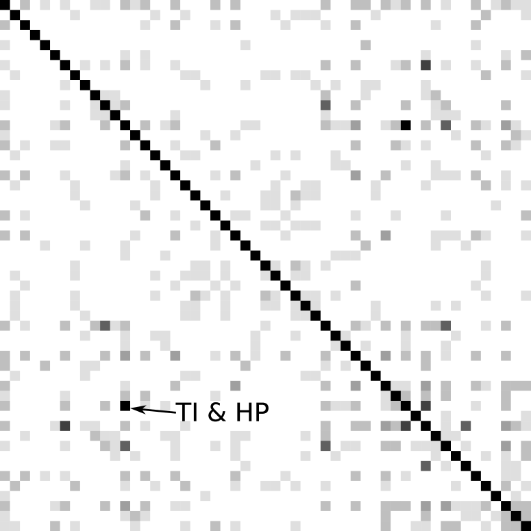
Figure 3: Heatmap of the support of the error component by LOREC from 2001-2009.

6 Discussion

In this paper, we propose a new covariance structure framework that recovers the covariance structures from many popular statistical models. The statistical performance is theoretically justified using various losses. We develop a first-order algorithm and prove the iteration complexity bounds of this algorithm. The merits of this new approach are illustrated using numerical examples.

One future direction is to further understand other theoretical properties under different norms, especially the minimax optimal rates. The Frobenius norm result here is conjectured to be minimax optimal using a similar argument from Rohde and Tsybakov (2011), but it remains to be rigorously justified. Moreover, the convergence rates are shown to be different under the Frobenius norm and the operator norm (Cai et al., 2010b), and it is interesting to study if such a phenomenon also exists under the covariance structure (1).

The results of course can be further improved with stronger structural assumptions. For example, we consider the factors to be unobservable. If one assumes that reasonable proxies are available, it is an interesting problem to incorporate such additional information, and improvements may be achieved hence. Moreover, the conditions imposed are to derive both support/rank recovery and matrix loss bounds. If one is interested in the joint matrix losses, without separating the two components, we suspect a different set of conditions shall suffice, for example Agarwal et al. (2011). Different conditions should also apply if one is only interested in determining the number of factors. Finally, it is also interesting to explore other extensions of general framework. For example, we will report the multiple spiked covariance model elsewhere.

The tuning parameters can be chosen theoretically as in the main results, or chosen using cross validation in practice. It is of great interest to study data-driven choices. We found that the development in Johnstone and Lu (2009) is particularly promising. On a related topic of estimating the inverse covariance matrix, we established the theoretical justification for using cross validation (Liu and Luo, 2012). In our low rank plus sparse setting, the analysis for data-driven penalties is still an open problem.

The convex optimization approach is adopted here to illustrate the framework, and for the computational efficiency reason. It is interesting to study adaptive versions of our proposal to ameliorate the bias. For example, one may replace the penalty function $\operatorname{pen}\left(\cdot\right)$ in (11) by either the adaptive lasso penalty (Zou, 2006) or the SCAD penalty (Fan and Li, 2001). We leave this to future work. It is also interesting to explore constrained versions of LOREC, because there were some improvements when estimating the inverse covariance (Cai et al., 2011).

Our algorithm may benefit further from incorporating additional numerical tricks, in order to improve the computation speed empirically. Currently full SVD is used for updating the low rank component. Partial SVD, such as partial Lanczos SVD, should suffice. In particular, it may provide additional numerical advantages for large scale problems. We plan to implement this in future releases of our package.

References

- Agarwal et al. (2011) Agarwal, A., Negahban, S., and Wainwright, M. (2011). Noisy matrix decomposition via convex relaxation: Optimal rates in high dimensions. arXiv preprint arXiv:1102.4807.
- Amini and Wainwright (2009) Amini, A. A. and Wainwright, M. J. (2009). High-dimensional analysis of semidefinite relaxations for sparse principal components. Annals of Statistics, 37:2877–2921.
- Anderson (1984) Anderson, T. W. (1984). An Introduction to Multivariate Statistical Analysis. John Wiley, New York.
- Beck and Teboulle (2009) Beck, A. and Teboulle, M. (2009). A fast iterative shrinkage-thresholding algorithm for linear inverse problems. SIAM Journal on Imaging Sciences, 2(1):183–202.
- Bickel and Levina (2008a) Bickel, P. and Levina, E. (2008a). Regularized estimation of large covariance matrices. Annals of Statistics, 36(1):199–227.
- Bickel and Levina (2008b) Bickel, P. J. and Levina, E. (2008b). Covariance regularization by thresholding. Annals of Statistics, 36(6):2577–2604.
- Bunea et al. (2011) Bunea, F., She, Y., and Wegkamp, M. H. (2011). Optimal selection of reduced rank estimators of high-dimensional matrices. The Annals of Statistics, 39(2):1282–1309.
- Cai et al. (2010a) Cai, J.-F., Candes, E. J., and Shen, Z. (2010a). A singular value thresholding algorithm for matrix completion. SIAM J Optim, 20:1956–1982.
- Cai and Liu (2011) Cai, T. and Liu, W. (2011). Adaptive thresholding for sparse covariance matrix estimation. Journal of the American Statistical Association, to appear., 106(494):672–684.
- Cai et al. (2011) Cai, T., Liu, W., and Luo, X. (2011). A constrained minimization approach to sparse precision matrix estimation. Journal of the American Statistical Association, 106(494):594–607.
- Cai et al. (2010b) Cai, T., Zhang, C., and Zhou, H. (2010b). Optimal rates of convergence for covariance matrix estimation. Ann. Statist, 38:2118–2144.
- Candes et al. (2009) Candes, E., Li, X., Ma, Y., and Wright, J. (2009). Robust principal component analysis. preprint submitted to Journal of the ACM.
- Chamberlain and Rothschild (1983) Chamberlain, G. and Rothschild, M. (1983). Arbitrage, factor structure, and mean-variance analysis on large asset markets. Econometrica: Journal of the Econometric Society, 51(5):1281–1304.
- Chandrasekaran et al. (2010) Chandrasekaran, V., Parrilo, P., and Willsky, A. (2010). Latent Variable Graphical Model Selection via Convex Optimization. Arxiv preprint arXiv:1008.1290.
- Davis and Kahan (1970) Davis, C. and Kahan, W. (1970). The rotation of eigenvectors by a perturbation. iii. SIAM Journal on Numerical Analysis, 7(1):1–46.
- Fama and French (1992) Fama, E. and French, K. (1992). The cross-section of expected stock returns. Journal of finance, 47(2):427–465.
- Fan et al. (2008) Fan, J., Fan, Y., and Lv, J. (2008). High dimensional covariance matrix estimation using a factor model. Journal of Econometrics, 147(1):186 – 197.
- Fan and Li (2001) Fan, J. and Li, R. (2001). Variable selection via nonconcave penalized likelihood and its oracle properties. J. Amer. Statist. Assoc., 96:1348–1360.
- Fazel et al. (2001) Fazel, M., Hindi, H., and Boyd, S. (2001). A rank minimization heuristic with application to minimum order system approximation. In American Control Conference, volume 6, pages 4734 –4739 vol.6.
- Fitzmaurice et al. (2004) Fitzmaurice, G., Laird, N., and Ware, J. (2004). Applied longitudinal analysis. Wiley-Interscience.
- Foster and George (1994) Foster, D. P. and George, E. I. (1994). The risk inflation criterion for multiple regression. The Annals of Statistics, 22(4):1947–1975.
- Friedman et al. (2008) Friedman, J., Hastie, T., and Tibshirani, R. (2008). Sparse inverse covariance estimation with the graphical lasso. Biostatistics, 9(3):432–441.
- Horn and Johnson (1994) Horn, R. and Johnson, C. (1994). Topics in matrix analysis. Cambridge Univ Pr.
- Huang et al. (2006) Huang, J., Liu, N., Pourahmadi, M., and Liu, L. (2006). Covariance matrix selection and estimation via penalised normal likelihood. Biometrika, 93:85–98.
- Jennrich and Schluchter (1986) Jennrich, R. and Schluchter, M. (1986). Unbalanced repeated-measures models with structured covariance matrices. Biometrics, 42(4):805–820.
- Ji and Ye (2009) Ji, S. and Ye, J. (2009). An accelerated gradient method for trace norm minimization. In Proceedings of the 26th Annual International Conference on Machine Learning, pages 457–464. ACM.
- Johnstone and Lu (2009) Johnstone, I. and Lu, A. (2009). On consistency and sparsity for principal components analysis in high dimensions. Journal of the American Statistical Association, 104(486):682–693.
- Koltchinskii et al. (2011) Koltchinskii, V., Lounici, K., and Tsybakov, A. B. (2011). Nuclear-norm penalization and optimal rates for noisy low-rank matrix completion. The Annals of Statistics, 39(5):2302–2329.
- Krim and Viberg (1996) Krim, H. and Viberg, M. (1996). Two decades of array signal processing research: the parametric approach. Signal Processing Magazine, IEEE, 13(4):67 –94.
- Ledoit and Wolf (2003) Ledoit, O. and Wolf, M. (2003). Improved estimation of the covariance matrix of stock returns with an application to portfolio selection. Journal of Empirical Finance, 10(5):603–621.
- Ledoit and Wolf (2004) Ledoit, O. and Wolf, M. (2004). A well-conditioned estimator for large-dimensional covariance matrices. Journal of Multivariate Analysis, 88(2):365 – 411.
- Leek and Storey (2007) Leek, J. T. and Storey, J. D. (2007). Capturing heterogeneity in gene expression studies by surrogate variable analysis. PLoS Genetics, 3(9):e161.
- Liu and Luo (2012) Liu, W. and Luo, X. (2012). High-dimensional sparse precision matrix estimation via sparse column inverse operator. arXiv preprint arXiv:1203.3896.
- Markowitz (1952) Markowitz, H. (1952). Portfolio selection. Journal of Finance, 7(1):77–91.
- Meinshausen and Bühlmann (2006) Meinshausen, N. and Bühlmann, P. (2006). High-dimensional graphs and variable selection with the lasso. The Annals of Statistics, 34(3):1436–1462.
- Nesterov (1983) Nesterov, Y. (1983). A method of solving a convex programming problem with convergence rate O (1/k2). In Soviet Mathematics Doklady, volume 27, pages 372–376.
- Nesterov and Nesterov (2004) Nesterov, Y. and Nesterov, I. (2004). Introductory lectures on convex optimization: A basic course. Kluwer Academic Publishers.
- Onatski (2009) Onatski, A. (2009). Testing hypotheses about the number of factors in large factor models. Econometrica, 77(5):1447–1479.
- Rohde and Tsybakov (2011) Rohde, A. and Tsybakov, A. B. (2011). Estimation of high-dimensional low-rank matrices. The Annals of Statistics, 39(2):887–930.
- Ross (1976) Ross, S. (1976). The arbitrage theory of capital asset pricing. Journal of Economic Theory, 13:341–360.
- Rothman et al. (2009) Rothman, A. J., Levina, E., and Zhu, J. (2009). Generalized thresholding of large covariance matrices. Journal of the American Statistical Association, 104(485):177–186.
- Sharpe (1964) Sharpe, W. (1964). Capital asset prices: A theory of market equilibrium under conditions of risk. The Journal of Finance, 19(3):425–442.
- Tibshirani (1996) Tibshirani, R. (1996). Regression shrinkage and selection via the lasso. Journal of the Royal Statistical Society. Series B (Methodological), 58(1):267–288.
- Wu and Pourahmadi (2003) Wu, W. B. and Pourahmadi, M. (2003). Nonparametric estimation of large covariance matrices of longitudinal data. Biometrika, 90(4):831–844.
- Yuan (2010) Yuan, M. (2010). High dimensional inverse covariance matrix estimation via linear programming. Journal of Machine Learning Research, 11:2261–2286.
- Zou (2006) Zou, H. (2006). The adaptive lasso and its oracle properties. Journal of the American Statistical Association, 101:1418–1429.