$Kepler$ Cycle 1 Observations of Low Mass Stars: New Eclipsing Binaries, Single Star Rotation Rates, and the Nature and Frequency of Starspots

Abstract

We have analyzed $Kepler$ light curves for 849 stars with T_eff $\leq$ 5200 K from our Cycle 1 Guest Observer program. We identify six new eclipsing binaries, one of which has an orbital period of 29.91 d, and two of which are probably W UMa variables. In addition, we identify a candidate “warm Jupiter” exoplanet. We further examine a subset of 670 sources for variability. Of these objects, 265 stars clearly show periodic variability that we assign to rotation of the low-mass star. At the photometric precision level provided by $Kepler$, 251 of our objects showed no evidence for variability. We were unable to determine periods for 154 variable objects. We find that 79% of stars with T_eff $\leq$ 5200 K are variable. The rotation periods we derive for the periodic variables span the range 0.31 $\leq$ P_rot $\leq$ 126.5 d. A considerable number of stars with rotation periods similar to the solar value show activity levels that are 100 times higher than the Sun. This is consistent with results for solar-like field stars. As has been found in previous studies, stars with shorter rotation periods generally exhibit larger modulations. This trend flattens beyond P_rot = 25 d, demonstrating that even long period binaries may still have components with high levels of activity and investigating whether the masses and radii of the stellar components in these systems are consistent with stellar models could remain problematic. Surprisingly, our modeling of the light curves suggests that the active regions on these cool stars are either preferentially located near the rotational poles, or that there are two spot groups located at lower latitudes, but in opposing hemispheres.

Key words: stars: low-mass — stars: late-type — binaries: eclipsing — stars: spots

1 Introduction

The $Kepler$ mission was designed to discover and characterize transiting exoplanetary systems (Borucki et al. 2010), and it has been quite successful with more than 1200 candidate systems already identified (Borucki et al. 2011). Perhaps equally exciting to the discovery and observation of exoplanets is the impact of high precision, long-term photometric observations on our understanding of ordinary stars. These new data are providing a wealth of information on the asteroseismology of stars similar to the Sun (e.g., Verner et al. 2011), as well as those objects in the classical regions of the instability strip (e.g., Benko et al. 2010).

It is also possible to use $Kepler$ to explore important, outstanding issues that remain for low-mass stars. One of the most important of these is that some of the measured fundamental parameters of low-mass stars (masses, radii, and T_eff) appear to be in conflict with values predicted by models. For example, analysis by L$\acute{o}$pez-Morales (2007) shows that the observed radii of low-mass stars are 10 to 20% larger than predicted by the stellar models of Baraffe et al. (1998). L$\acute{o}$pez-Morales found that there was a clear correlation between the activity levels of short period (P_orb $\sim$ 3 d) binaries and the discrepancy in the radii of the stellar components. Morales et al. (2008, 2010) suggest that either the models are flawed, or that differences in metallicity, magnetic activity, or the presence/distribution of star spots make such comparisons moot. If the larger radii observed for the components in short period binaries is indeed due to enhanced magnetic activity as a result of tidal locking, then it is suspected that the low mass stars in binaries with orbital periods longer than $\sim$ 10 d should have radii in agreement with models. The main issue that existed before the launch of the $Kepler$ mission was the lack of long period (P_orb $>$ 10 d), low-mass eclipsing binaries. The samples used to arrive at the results above relied on a handful of shorter period eclipsing binaries. It is well known (Bopp 1987, Radick et al. 1987) that rapidly rotating low-mass stars are intrinsically more active, and thus if the components in short period eclipsing binaries are spun-up by gravitational interactions (Zahn 1977, 1994), then their value for comparison to more slowly rotating isolated field dwarfs is diminished.

It would be extremely useful to discover additional low-mass eclipsing binaries with longer periods to investigate whether these more slowly rotating objects might be used to constrain stellar models. This was the genesis for our Cycle 1 and 3 $Kepler$ programs that proposed to obtain light curves for 2400 cool (T_eff $\leq$ 5200 K) stars to search for previously unknown long period, low-mass eclipsing binaries (LMEBs). As we discuss below, we have been successful in identifying an LMEB that has a period of 29.91 d, along with five shorter period LMEBs in our Cycle 1 data. This success rate is in line with our assumption that the mean binary star fraction is 35% for K and M dwarfs (Mayor et al. 1992, Leinert et al. 1997, and Fischer & Marcy 1992).

Along with the discovery of new LMEBs, the $Kepler$ light curves from our program objects provides an unprecedented data set to investigate the variability of an unbiased sample of low-mass main sequence stars on timescales of $\sim$ 90 d. For example, we can use the modulation of the light curves induced by starspots to determine the rotation rates for these stars, and compare them with predictions for the angular momentum evolution of such objects (e.g., Krishnamurthi et al. 1997). It is also possible to investigate the nature of stellar activity for low-mass stars to levels not previously attainable using ground-based photometry. With a large sample of objects with continuous light curves spanning 90 (or more) days, we can probe the longevity of the active regions on these low-mass stars, and attempt to unravel the latitudinal (and/or longitudinal) distribution of starspots on these objects.

In the following we discuss the selection of our targets and the reduction of the Cycle 1 $Kepler$ light curves in section 2, discuss the discovery of the new LMEBs and derivation of the stellar characteristics in section 3, and discuss our conclusions in section 4.

2 Observations

Our sample of objects for observation in Cycle 1 (which ran from 2009 June 20, until 2010 June 23) was selected using the stellar parameters available in the Kepler Input Catalog (the “KIC”, Brown et al. 2011). With multi-band photometry ($griz$, “DDO51”, and $JHK$ from 2MASS), Brown et al. were able to assign values of T_eff, log($g$), A_V, and estimate the metallicity for more than 4 million objects in the $Kepler$ field-of-view (note: see the discussion in Brown et al. for important caveats on each of these derived parameters). From the KIC for Cycle 1, we constructed a list of all of the stars that had T_eff $\leq$ 5200 K, $r$ $\leq$ 17.0, log($g$) $\geq$ 4.0, A_V $\leq$ 0.5, and that were not already designated as $Kepler$ program stars. In addition, we only selected targets that had no neighboring objects within 6” of our sources. There were 1239 objects that met these criteria. Dropping the faintest 39 sources, we ended up with a list of 1200 targets. The brightnesses of our observed targets spanned the range 15.16 $\leq$ $r$ $\leq$ 16.97.

Our proposal sought to obtain “long cadence” (30 min) light curves spanning 90 days (a single $Kepler$ “Quarter”) for 1200 late-type dwarfs. Unfortunately, due to a mission programming error, only 849 unique targets were observed during Cycle 1. This did mean, however, that 260 targets were accidentally re-observed in a second quarter. In nearly all these cases we obtained two quarters of data that spanned three quarters, skipping the middle quarter (e.g., quarter 2 + 4, or quarter 3 + 5). This separation allowed us to examine the light curves for coherent variations on timescales of up to 270 days, and is especially useful in searching for very slowly rotating stars.

2.1 Extraction of the Light Curves

The “Pre-search Data Conditioned” (PDC) light curves released to Guest Observers (GOs) have been processed through the $Kepler$ pipeline (see Jenkins et al. 2010). After careful examination, the process used by the $Kepler$ team appears to introduce artifacts, and/or remove valid photometric variations. Part of the reason for this is that the drift for some stars during a quarter was large enough that significant flux was lost out of the optimal photometric aperture used by the $Kepler$ pipeline to produce the light curves. While the fine guidance sensors on $Kepler$ generally keep the pointing to within $\pm$ 0.05 pixels, the effects of differential velocity aberration as the telescope orbits the Sun introduces an annual motion of 6” on the $Kepler$ field-of-view. Subsequent polynomial fits to remove such trends appears to both introduce, and eliminate, photometric variations. Since it is impossible for a GO to reconstruct the process for any of the program targets, we decided to build our own processing pipeline that starts with the complete set of calibrated, sky-subtracted postage stamp images released to the GOs in early 2011.

The default photometric aperture assigned to each target depends on the source brightness, and usually spans several pixels. This central aperture is then surrounded by a “sky” region. For the faint stars of our program, the resulting postage stamp images were usually 3 $\times$ 5 or 4 $\times$ 6 pixels in size. Preliminary investigations showed, however, that a significant portion of the stellar flux was not contained within the pre-defined apertures for our targets. Thus, some of the stellar flux could often be detected in the “sky” pixels that surrounded every target’s aperture. This is partially due to the large point spread function of the defocussed images produced by $Kepler$, but mostly due to positional drift over the quarter. The result was that the PDC light curves have systematic variations due to improper “sky” removal, and too small of a photometric aperture.

As a result, we decided to sum-up the flux in all of the pixels in each postage stamp image to get a better handle on the light curve of a source. We found this process alone dramatically reduced the presence of the large scale systematics noted above. The main drawback to this method is that flux from nearby stars can often contaminate the resulting light curve. In the cases where this background severely contaminates the light curve of our program object, we define those light curves as suffering from “third light” contamination. As noted below, many times such contamination can be non-varying, and be accounted for in extracting the target light curve. In other cases, it is impossible to determine which object in the FOV is the source of the variations. To better avoid such issues we would recommend that future observers of faint targets increase the nearest neighbor radius to $>$ 12” if there are any nearby stars that might provide sufficient contaminating flux (i.e., stars as bright, or brighter than the target). The light curves generated by the summing process are then (only) used to determine the mean flux value for that source during the quarter.

After the flux summing process, the systematics in the light curve due to positional drift are greatly reduced, but pixel-to-pixel sensitivity, both in spectral response, as well as quantum efficiency, and intrapixel variations, can produce significant systematics. To account for these, we performed a Principal Component Analysis (PCA; Murtagh & Heck 1987) on the ensemble of post stamp images for each source. The PCA process correlates the variation of the flux in each pixel with the fluxes in all of the other pixels in the image. We then subtract the most significant principal component from the light curve and scale it using the mean of the summed light curve to conserve flux. This latter step is done so that we can obtain light curve amplitudes that are calibrated to the $Kepler$ system. In this way, the effects noted above are largely accounted for, and the result is a relatively clean light curve.

To demonstrate the process we present light curves for three targets in Fig. 1. In the top panels of this figure are the PDC “calibrated” pipeline processed $Kepler$ light curves as delivered to GOs. It is clear from the pipeline processed light curve that Kepler ID#8016381 (Fig. 1a) shows periodic variations, but they are somewhat irregular. The summed and PCA-processed light curves are much more symmetric. In the case of K8016381, these latter two light curves are identical. This result is due to the fact that the centroid of this star only moved a tiny fraction of a pixel over the 90 d quarter. In contrast to K8016381 is the light curve for K5428432 (Fig. 1b). The PDC pipeline processed light curve suggests a possible slow, periodic variation with a significant amplitude. Our PCA processing reveals what appears to be a much more rapid oscillation of lower amplitude. As shown in the centroid plot, however, this star appeared to have numerous jumps in its position, and nearly every one of these is imprinted on its light curve. These glitches have a variety of origins, from focus changes, to cosmic ray hits, all of which are discussed in Jenkins et al. (2010). In the following, all light curves from sources with large and choppy centroid motion have been removed from our rotation/starspot analysis. Such light curves remain useful for discovering LMEBs, exoplanet transits, or for short period asteroseismology investigations (see Garcia et al. 2011 for one possible method to correct these types of light curves).

As mentioned above, some of our objects suffer from third light contamination. Such contamination is easily identified by examining the motion of the centroid. As shown in Fig. 1c, if the motion of the centroid of the star reflects the variability seen in the light curve, there is significant third light contamination. The amount of such contamination varied from an insignificant level, up to to the point where it was so dominant as to render the light curve useless. Where we felt that a light curve was only marginally affected, it was included in the analysis program, otherwise it was discarded. There was no defined rule for such decisions, given the great range in behavior exhibited by our program objects but, generally, if the third light imparted centroid motion on order of $\pm$ 0.01 pixels, it was deemed to be problematic. Of the 849 light curves that comprised our Cycle 1 survey, 173 were dropped from further analysis either due to third light contamination (33), or from multiple large, abrupt changes in the centroid motion (140).

2.2 Light Curve Classification

The $Kepler$ PDC pipeline-processed light curves, even with the flaws noted above, were sufficient to search for eclipsing binaries. From the 849 targets of our sample we identified six eclipsing binaries (two of which are almost certainly W UMa variables). These objects, along with their derived parameters, are listed in Table 1. After discarding the unusable light curves, we proceeded to analyze the light curves to classify the objects as periodic variables, probable periodic variables of long period, aperiodic variables, and objects showing no variability. We define periodic variables as objects that display either two similar, symmetric maxima with one minimum, or two minima with one maximum in their light curves (which either spanned 90, 180, or 270 d). Long period variables were objects that clearly showed evidence for both a minimum and a maximum, but the light curves were of insufficient duration to reveal a second maximum (or minimum). Aperiodic variables were objects with complex light curves that ranged from quasi-periodic, to chaotic. Non-variables were obviously objects that showed no significant variability. We found that we could generally detect symmetric oscillations that had amplitudes of $\sim$ 10 counts peak-to-peak in light curves that have mean fluxes of $\sim$ 2000 counts. Thus, non-variables are objects whose periodic variability has a total amplitude below $\sim$ 0.5%. These objects could be aperiodic, but at this level, tiny centroid changes can impart aperiodic features in the light curves, making such classification impossible. Of the 670 light curves analyzed for variability, we found 265 periodic variables (Table 2), 126 long period variables (Table 3), 28 aperiodic variables (Table 4), and 251 non-variables (Table 5).

2.3 The Sample

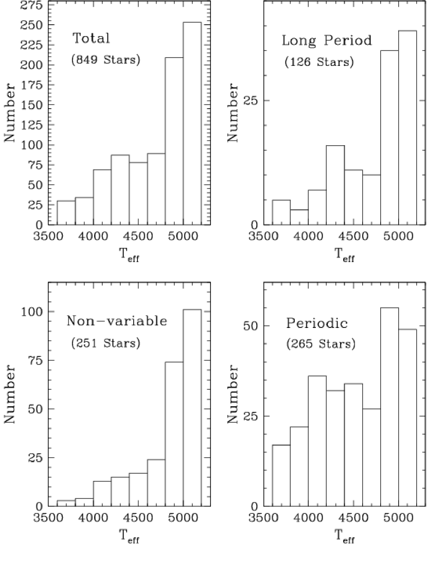
Figure 2: A histogram showing the temperature distribution of the entire sample (top left panel), the non-variable objects (lower left panel), the long period variables (top right panel), and the periodic variables (bottom right) sorted into 200 K bins.

After classification, we can examine the types of stars found in each group. A histogram of the temperature distribution of our entire sample of 849 objects can be found in the top-left panel of Fig. 2. Our sample is dominated by early K dwarfs. Our hottest stars have T_eff = 5200 (K0V), and our coolest objects have T_eff = 3500 K (M2V). Histograms of the temperature distributions of our long period variables, and the non-variable objects, are shown in the top-right, and bottom-left hand panels, respectively, of Fig. 2. The histogram for the long period variables closely resembles that of the overall sample, while the histogram for the non-variable objects is dominated by hotter stars. It is clear that nearly all stars with T_eff $\leq$ 4000 K are variables at the level detectable with $Kepler$. This is reflected in the histogram for the sample of periodic variables (bottom-right panel of Fig. 2) that demonstrates periodicities are more likely to be found in cooler stars. Basri et al. (2011) have performed a statistical analysis of the entire sample of 150,000+ program stars observed during Q1, and found that 87% of their (6522) stars with temperatures below 4500 K were variable. We find that 79% of our sample of (298) stars with T_eff $\leq$ 4500 K are intrinsic variables.

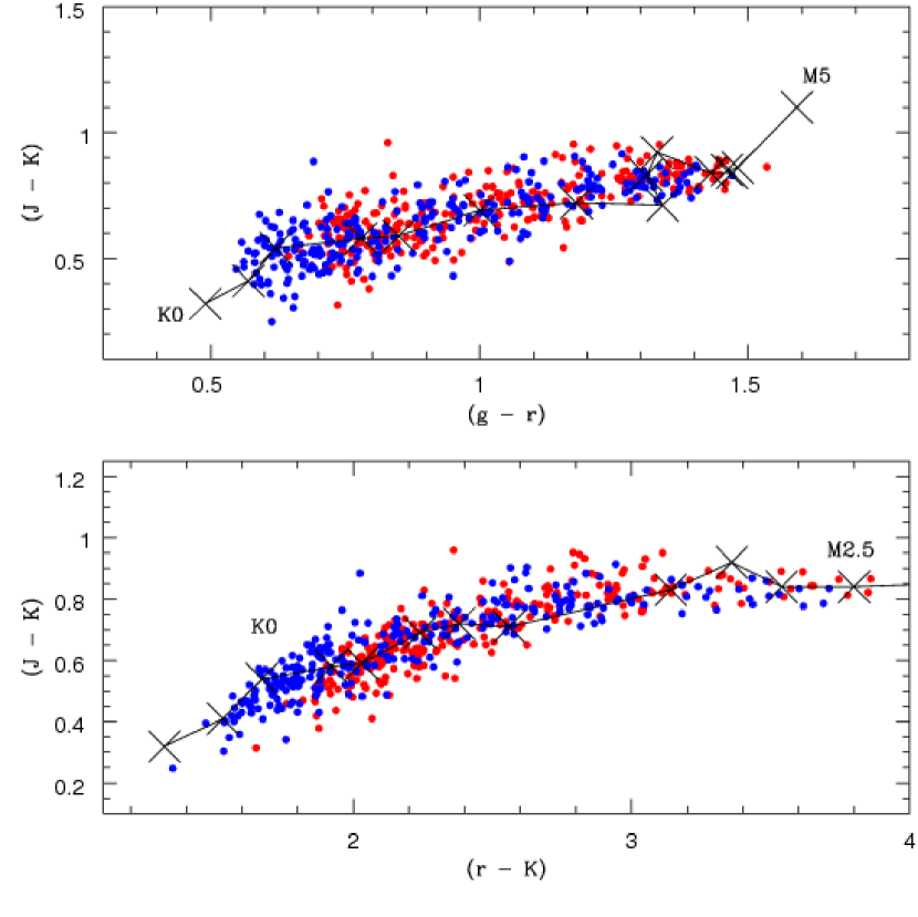
Figure 3: Color-color diagrams for the periodic variables in our sample. The red symbols are the unreddened positions of the objects, while the blue symbols have been dereddened using the tabulated values of E($B-V$) from the KIC. In each panel, we have plotted crosses at the locations for main sequence stars using the tabulation of synthetic SDSS/2MASS photometry for solar metallicity standards from Covey et al. (2007).

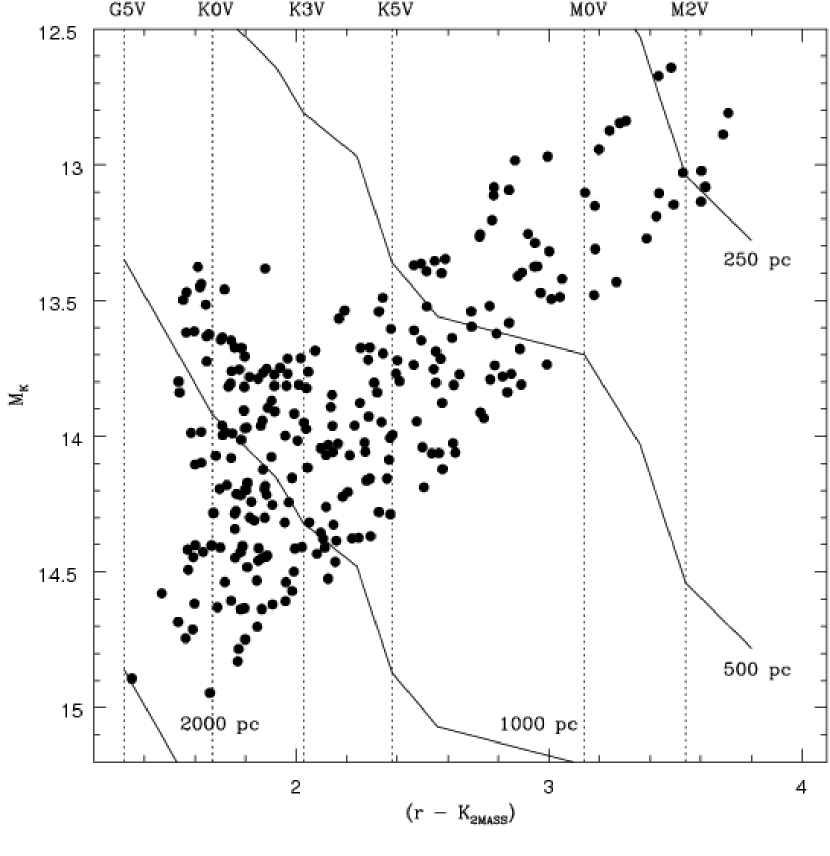
Figure 4: An HR diagram for the periodic variables constructed by converting the ($r$ $-$ $K$) color listed in the KIC into spectral type using Covey et al. (2007), after accounting for the tabulated extinction. The absolute visual magnitudes of dwarfs earlier than K5V have been taken from Houk et al. (1997), and those later than K7V have been taken from Bessell (1991). The absolute visual magnitudes were converted to M_K using the tabulated ($V$ $-$ $K$) colors of these stars in Bessell (1991) and Johnson (1966).

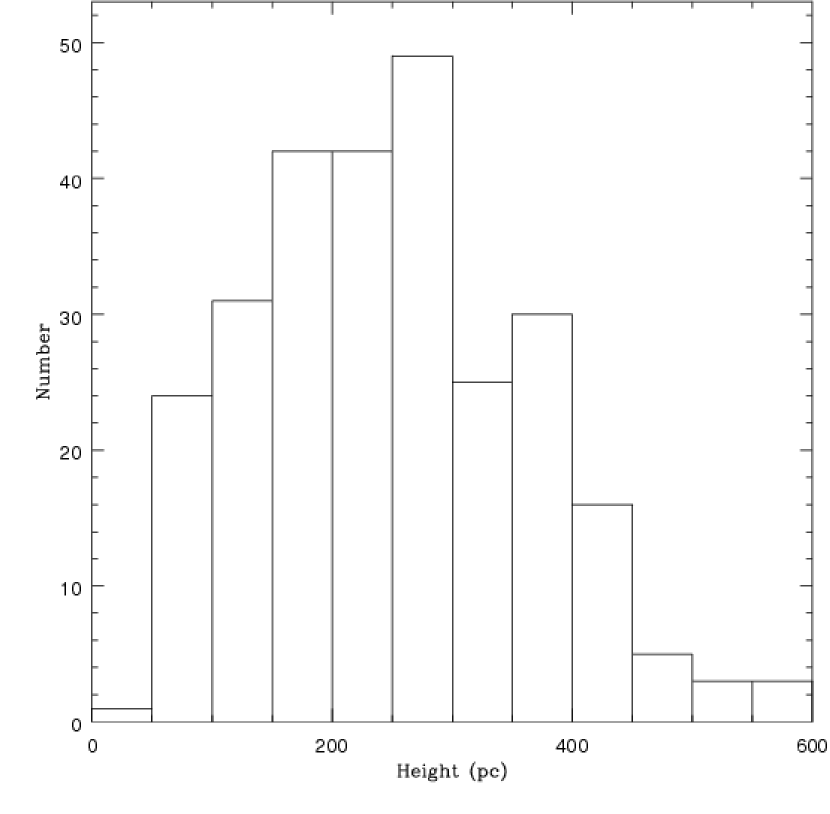
Figure 5: A plot of the scale height distribution for the (265) periodic variables (note that one object has a scale height of 815 pc, and is outside the limits of this plot). The mean scale height is 249.9 pc.

Since the stellar activity level increases as one descends the main sequence, it is obvious that rotational modulation of the light curve due to starspots is what is driving the majority of the periodic variations. We will discuss this assumption in the next section. To better characterize the periodic sample, we present a color-color plot of these objects in Fig. 3. Even with the caveats in the assignment of T_eff in the KIC ($\pm$ 200 K, or roughly one spectral type) noted by Brown et al. (2011), our set of periodic variables clearly has the desired high temperature cutoff near a spectral type of K0V. An HR diagram (Fig. 4) of the periodic variable sample indicates that most of these objects are early to mid-K dwarfs with distances near 1 kpc. The height above the galactic plane of our periodic variable sample is shown in Fig. 5. The mean scale height of our sample is 249.9 pc. This is consistent with an “intermediate disk population” (e.g., Ng et al. 1997) with a mean age near 5.75 Gyr. Thus, this group of periodic variables should be dominated by objects similar to the Sun in both age and metallicity.

2.3.1 Determining Rotation Periods

We will assume that the periodic modulations in the observed light curves of our sample of late-type stars is due to rotation. The association of photometric modulations in late-type stars with starspots dates back to at least Kron (1947). Vaughan et al. (1981) obtained long term Ca II H and K photometry of a sample of ninety one F to M stars that showed days, to month long variations, in nearly all of their stars. Twenty of these stars clearly showed evidence for rotational modulation with periods ranging from 2.5 to 54 days. They found that these rotation periods were consistent with spectroscopic determinations of the ($v$sin$i$) rotation rates for their stars, confirming rotation as the source of the photometric variability. These results demonstrate that, unlike the Sun, large regions of stellar surface activity can last for several rotation periods. Dorren & Guinan (1983) observed several of the stars from Vaughan et al. in both narrow-band and intermediate-band filters to sample both the blue continuum, and H-alpha spectral regions. For their most variable object (HD149661, K0V), total variations of 4% in the blue, and 2% in the red continuum filters were observed. Interestingly, they found that both the H-alpha and Ca II emission were anticorrelated to the continuum fluxes. They conclude that the photometric modulations were due to dark spots on these stars (all of which probably have significantly higher levels of chromospheric activity than seen on the Sun).

To determine the rotation rates for our set of periodic variables we have used Period04 (Lenz & Breger 2005) to perform Fourier analysis to identify the dominant frequencies in each light curve. One of the nice features of Period04 is the ability to remove low frequency modulations of the light curves to produce “pre-whitened” light curves to precisely identify the period of the larger amplitude modulations. There are numerous examples in our periodic variable data set where the dominant periodic amplitudes are slowly modulated by a longer term variation that is intrinsic to the star. In some cases this appears to be due to changing starspot size, while in others it is simply a global change in the continuum level. For most objects, such slow modulations were fit with a single minimum or maximum of a sinusoidal variation that had a period that was many times longer than the duration of the light curve.

In addition, there are a number of objects that show more complex light curves, with a second period that could be identified. We believe that for the majority of objects, this is due to a separate starspot group that is present on the star. In some cases, the periods for these second modulations are identical to the primary modulation period, but are simply offset in phase. In other sources, however, the second period is different to the primary period. We believe that the best explanation for such period differences is differential rotation.

3 Results

The main goal of our program was to identify new LMEBs with periods in excess of 10 days so as to test whether rotational spin-up was the genesis for the discrepancy between the observed radii of low-mass stars, and predictions from stellar models. From our Cycle 1 data we identified six new LMEBs. Two of these objects, K636722 and K8086234, are almost certainly W UMa variables, and technically not LMEBs. One of these six, K6431670, has a period in excess of 10 days (see Table 1). Given that before the launch of $Kepler$ the longest known period of an LMEB was 8.4 d (Devor et al., 2008), this new object certainly met the program goals. This finding, however, is overshadowed by the results from analysis of the $Kepler$ public release data from Q1. Coughlin et al. (2011, see also Pr$\check{s}$a et al. 2011) identified 231 eclipsing binaries in this data set where the primary star is cooler than the Sun. Twenty nine of those LMEBs have periods longer than 10 d. As the majority of those systems are several magnitudes brighter than K6431670, they are much better binaries for determining whether the components in long period LMEBs have radii in line with the predictions from models. We are currently obtaining radial velocity and multi-wavelength light curves for a subset of these 231 objects to allow for further investigation of this issue.

As noted above, the six LMEBs we have discovered are within expectations for our sample size. Mayor et al. (1992) estimate a binary fraction of 45% for K dwarfs, while for M dwarfs the binary fraction estimate ranges from 25% (Leinert et al. 1997) to 42% (Fischer & Marcy 1992). In a complete, and unbiased survey, Delfosse et al. (2004) found a binary fraction of 26 $\pm$ 3% for M dwarfs. Since our sample draws from a mixture of these two spectral types, we would expect binary fractions of $\approx$ 35%. The orbital period distribution for late type stars is not very well known, but Fischer & Marcy (1992) found a peak centered at 9 yr for M dwarfs. Their result resembled that for G stars, which have a Gaussian distribution centered at $\langle$P_orb$\rangle$ = 173 $\pm$ 8.6 yr (Duquennoy & Mayor 1991). Putting these data together, assuming $\langle$P_orb$\rangle$ = 9 $\pm$ 8.6 yr, and a main sequence radius relationship, we estimate that in a sample of 849 stars, we would expect to find five low mass eclipsing binaries.

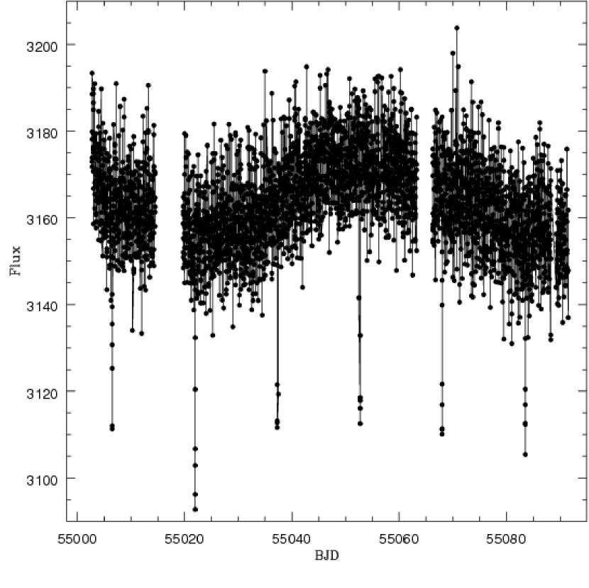
Figure 6: The PCA corrected light curve of K6431670, the host of a candidate exoplanet that has an orbital period of 15.4 d.

In addition to the six LMEBs detected in our survey, we also discovered a candidate exoplanet system: K5164255 ($r$ = 16.37, designated as KOI824.01 by the $Kepler$ team). This object is probably a “warm” ($\sim$ 650 K) Jupiter due to its moderate orbital period (P_orb = 15.4 d), and the fact that the host star primary is a K3V (T_eff = 4829). Our modeling of the $Kepler$ light curve for this object, presented in Fig. 6, using JKTEBOP (Southworth et al. 2004a,b) leads to the parameters for the host star and planet listed in Table 6. Given the large number of such objects detected by $Kepler$, this object is of little interest for further investigation due to the faintness of its host star, which is below the capabilities of current radial velocity studies.

3.1 Rotation Rates of Low Mass Stars

We have assumed that the periodic modulation seen in the light curves (e.g., Fig. 1) is the rotation period of those stars. In Table 5 we list the periods of the dominant modulation found from fitting the light curves using Period04. The derived periods range from 0.31 d to 126.5 d, with a mean of 32.12 d. We present a plot of rotation period vs. T_eff in Fig. 7. The resulting distribution is remarkably flat (the means in 200 K bins are also plotted).

As discussed earlier, rotation of a spotted star is the obvious interpretation for the modulations we detect in the light curves of our late-type dwarfs. As shown by Christensen-Dalsgaard & Frandsen (1983), solar-like oscillations in late-type dwarf stars have similar pulsation periods as the Sun ($\sim$ 5 min), with amplitudes of a few parts-per-million. Such oscillations could never be seen in the $Kepler$ long duration light curves. Gilliland (2008) has shown that red giants have variability on these time scales, but those variations have a recognizable photometric signature. Basri et al. (2011) investigated this aperiodic signature to see if it is possible to select giants vs. dwarfs based upon their $Kepler$ light curves alone. They found that the selection process was robust, with only a few high gravity objects showing up in their analysis as red giants. Basri et al. suggest that it is possible that these few objects are actually red giants that were misclassified as dwarfs in the KIC. This process demonstrates that the gravities listed in the KIC are fairly reliable for late-type stars.

The light curves of red giants can show quasi-periodic behavior that are similar in nature to the oscillations seen in the Sun, except for their longer periods and much greater amplitudes (see Huber et al. 2010). We attempted to fit periods to all objects whose light curves might be periodic. Only after we could not identify a period consistent with the entire light curve were those objects re-classified as aperiodic. It is highly likely that no red giants remain in our “rotation” sample.

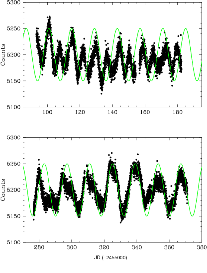
Figure 8: A plot of the light curve for K10200948 for Q3 (top panel) and Q5 (bottom panel). The green sine wave plotted in both panels has identical phasing at the rotation rate tabulated for this object. Clearly this object has one major spot group that maintains a coherent phasing while one, or more, additional spot groups is rapidly evolving in size, and/or moving in phase relative to the dominant group.

It is possible, however, that the period we determine for the rotation rate is an even multiple, or fraction, of the true period. Shown in Fig. 8 is an example of an object (K10200948) that has one of the more complicated, and rapidly evolving light curves of any of the sources in our sample. In the Q3 data, analysis using Period04 finds a period of 7.197 d. In the Q5 data, we find the dominant period to be 14.45 d. Analysis of the combined light curves results in a best-fit period of 14.006 d. This latter period is what is over-plotted on the light curves shown in Fig. 8, and is what we assign as the rotation period for this object. Clearly, additional spots are present on K10200948 that are moving/evolving relative to the “main spot group” responsible for the coherent oscillation that retains the exact same phasing over 270 d. Fortunately for this target we have two quarters of data that allows us to isolate the “correct” period for this target. It is obvious, however, that there could be a few cases where similar sets of starspot groups are found to be centered on opposite hemispheres so as to create confusion about the true period. It is also obvious that if differential rotation is present, as suggested by the changing shapes of the maxima in the light curve of K10200948, the period we derive could be incorrect due to the slow migration of the main spot group. Since we have no secondary information as to the inclination of the rotational axis of these stars, it is impossible to know the exact latitude of these active regions, or whether the large spot groups are actually changing position with time, or are simply evolving in size and/or shape.

Another possible effect that could cause errant periods is evolution of a starspot group on a timescale similar to the rotation period. If the stellar activity was somehow constrained to evolve at certain discrete longitudes, then the appearance, or disappearance, of spot groups with lifetimes similar to the rotation period could lead to erroneous period determinations. This is most true for the longest period systems. Instead of rotation, these light curves could be modeled by the repeated growth and decay of a fixed single spot group on a non-rotating star. Hopefully, nature is not this cruel, but since our knowledge of stellar activity cycles and the rotation rates of low-mass field stars is still primitive, it is impossible to rule out such behavior.

3.2 Amplitude of the Spot Modulation

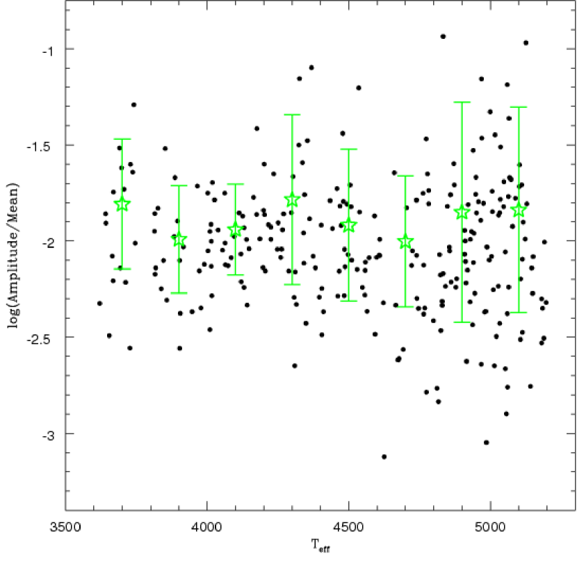
Figure 9: The (log) of the ratio of the peak-to-peak amplitude to the light curve mean plotted vs. T_eff for our periodic variables. The means in 200 K bins are plotted as green stars with error bars.

Tabulated in Table 5 are the amplitudes of the modulations for our sample of periodic objects. The amplitude listed there is the largest peak-to-peak variation seen in the light curve of that object. We plot the distribution of these amplitudes with respect to temperature (as well as their means) in Fig. 9. Surprisingly, this distribution is flat, with the early K dwarfs showing a greater range in modulation than the M-type dwarfs. The temperature-dependent means (in 200 K bins), however, are consistent with a single value (the sample mean was 1.3%).

The level of variation seen here is consistent with the observations of Dorren & Guinan (1983), suggesting that our sample of rotating stars has a higher level of activity than exhibited by the Sun. However, it is important to realize that a nearly equal number of stars in our survey were found to exhibit no variations, though even those stars could be more active than the Sun. Treating the Sun as a variable star using the VIRGO instrument on SOHO, Lanza et al. (2004) show that the white light (similar to $Kepler^{\prime}s$ filterless response function, see below) variations during solar maximum are of order of 500 ppm (see also Pagano et al. 2005), a factor of ten smaller than our detection limit of $\sim$ 0.5%.

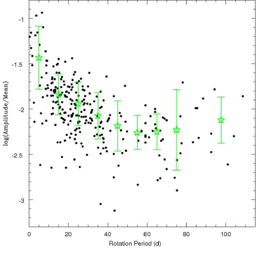
Figure 10: The (log) of the peak-to-peak amplitude of the periodic variables vs. the rotation period. The green stars with error bars are the means in 10 d bins (except for the final point which contains all objects with rotation periods greater than 80 d).

It is also interesting to examine the rotation period-activity relationship. In Fig. 10 we plot the amplitude of the variations vs. the rotation period for our sample of periodic variables. It has been well established that younger stars rotate more quickly, and that these objects display a higher level of activity (c.f., Radick et al. 1987). This trend is observed in our sample, where the most rapid rotators generally show larger photometric modulations. At periods longer than $\sim$ 25 d, the trend flattens dramatically. We discuss the implications of this result in the next section.

3.3 Spot Modeling of the Light Curves

Without additional observations, it is difficult to derive the inclination angles of the rotational axes for any of the stars in our sample. Statistically, the mean inclination angle for a random sampling of rotating stars is $i$ = 57^∘. There are two light curve morphologies that can be generated using a single spot: continuously variable (sinusoidal), and flat maxima. Continuously variable light curves occur when the starspot is “circumpolar” in the sense that it is always in view for the observer. Flat-maxima light curves occur when the spot is out of view for some fraction of the rotation period. It is interesting to examine what the break-down into these two categories might imply for the latitudinal distribution of spots.

We have examined the light curves of all our rotation targets, and have classified them into the following groups: flat-maxima (90 objects), continuously variable (119), flat-minima (40), and complex (16). A flat maximum light curve simply has maxima that are broader than the minima seen in that light curve. Flat minima light curves are the opposite to flat maxima. Continuously variable light curves have minima and maxima that have nearly identical shapes. Complex light curves have such dramatically changing spot groups that it is not possible to identify a consistent portion of the light curve that allows classification into the one of the other three categories. Complex and flat minima light curves cannot be explained using a single spot. A light curve with a flat minimum suggests that a second spot, with similar properties, rotates into view as the first spot is passing out of view. The flat-minima light curves in our sample always have non-flat maxima.

The fact that 57% of our rotation sample have continuously variable light curves suggests that for the majority of our objects the sum of the inclination angle ($i$) and the starspot co-latitude ($b$, formally defined below) is less than 90^∘. This relationship simply states that the starspot remains in view at all times (especially given that a starspot must subtend an appreciable angle to be detectable, see below). If we assume a random set of rotational inclination angles (0.0 $\leq$ $i$ $\leq$ 90.0), and a random value for the starspot’s co-latitude (0.0 $\leq$ $b$ $\leq$ 180.0), we find that statistically, only 21% of our stars should have continuously variable light curves. Assuming single, dominant spot groups, this result would strongly argue for “polar” spots. The only alternative to this conclusion is that many of our stars have two spot groups in diametrically opposite hemispheres with similar enough properties to create continuously variable light curves. The fact that 40 of our stars have flat minima, an indicator for two very similar spot groups, indicates that this latter conclusion may have some validity.

We can attempt to model the light curves of our rotating stars to investigate starspot sizes and distributions, but before we do so, it is important to establish what effect the broad bandpass of the $Kepler$ mission has on the detection of cool spots. Basri et al. (2010) have investigated the variability of solar-like stars with an emphasis on comparison to the Sun. They found that the $g+r$ light curves from the VIRGO instrument on SOHO essentially reproduces the broad $Kepler$ bandpass. Thus, the minima in the $Kepler$ light curves of cool stars are due to dark spots on the surface, and thus we are not seeing maxima due to bright faculae (that actually cover a larger fraction of the solar photosphere than spots). As discussed in Knaack et al. (2001), faculae have a higher contrast near the limb of the Sun in the visual bandpass. In contrast, sunspots have a higher contrast when located near the center of the solar disk. Knaack et al. investigated whether viewing the Sun from higher inclination angles would result in a greater photometric variation, making the Sun more consistent with the larger variability observed for field stars like the Sun. They found that changing the Sun’s inclination has only a modest ($\sim$ +6%) effect on the solar irradiance. Thus, the $Kepler$ light curves should be useful for constraining the properties of starspots for our sample of randomly inclined, rotating stars.

To investigate the starspot parameters for the objects in our rotational sample we have modeled the $Kepler$ light curves using PHOEBE (Pr$\check{s}$a & Zwitter 2005), a graphical interface to the Wilson-Divinney binary star light curve modeling code (see Kallrath et al. 1998). We use PHOEBE for modeling single stars due to the fact that the most recent version has been adapted for the $Kepler$ mission (with new stellar atmosphere models and limb darkening coefficients). We simply set the orbital period of the binary to the rotation period, and turn-off the light from the companion star.

With limited details about our stars, there are few constraints on the input parameters used in light curve modeling. In the following, we have assumed that our objects are main sequence dwarfs with the masses, radii, and log$g$ expected for stars with the T_eff listed in the $KIC$. There are four relevant parameters for adding a spot to generate a light curve using PHOEBE: the spot longitude, co-latitude, radius, and temperature (input as the ratio T_spot/T_eff). Co-latitude has its normal meaning in that it is the angle between the pole of the star, and the center of the spot. Radius is the angular radius of the spot as measured at the center of the star. The minima in light curves for stars with a single spot are driven mostly by the interplay between the inclination angle and co-latitude, and less by spot size and temperature contrast, which are somewhat, but not fully, degenerate. PHOEBE assumes round spots of uniform temperature.

To demonstrate the difficulties with ascertaining the exact spot distributions for any one light curve, we return to K10200948. First, if we were to classify the Q3 light curve for this object, we would have deemed it “continuously variable”. The Q5 light curve, however, shows it to have flat-maxima for the last four maxima (and a flat minimum for the first part of the light curve!). Obviously, this type of issue could erupt for every object in our sample through the appearance and/or disappearance of a second spot.

In Fig. 11a we present the Q5 light curve for K10200948 phased to its rotation period. It is clear that the phasing cleans-up most of the light curve, and it emphasizes the flat-topped nature of its maxima. We found that the best fit, one spot model (middle panel) for this light curve occurs with an inclination angle of $i$ = 70^∘, and a co-latitude of $b$ = 45^∘. For this model the spot has a radius of 10^∘, and a temperature ratio $w$ = 0.89. At larger co-latitudes the shoulders on the minima are too square, at smaller co-latitudes the model light curves are too sinusoidal. There is a set of models with $i$ $\approx$ 50^∘ and $b$ $\approx$ 60^∘ that fit equally well. In both families of models, the spot transits a similar line-of-sight chord ($i$ + $b$ $\sim$ 110^∘). In all spot models the shoulder on the light curves disappears for $i$ + $b$ $\leq$ 90^∘. As noted above, these are circumpolar spots that never fully disappear for the viewer, leading to continuously changing light curves.

In Fig. 11b we present the phased Q3 light curve for K10200948. The rapidly changing maxima during this quarter results in a messier phased light curve, but shows relatively symmetric minima and maxima at roughly twice the rotation period. To model this light curve we added a second spot at a longitude that is located 175^∘ from the spot used to model the Q5 light curve. For the resulting models we assumed that both spots had identical co-latitudes. Again, the best fitting model was one with an inclination angle of $i$ = 70^∘, and a co-latitude of $b$ = 45^∘. Both spots had the same radius, 12^∘, slightly larger than found for the one spot model while at the same time having slightly higher temperature ratios: $w$ = 0.91. Changing spot size affects the total continuum level. Close inspection of Fig. 8 shows that the peaks of the maxima in Q5 were slightly larger, and thus the size of the spots needed to be increased to lower the overall flux level seen in the maxima of the Q3 light curve (note: small changes in the normalization between the two quarters could be the source of this issue). Meanwhile, the flux level of the minima remained similar, so the spots needed to be “less dark” (hotter) to fit these minima. As with the single spot model, an additional family of models with $i$ $\sim$ 50^∘, $b$ $\sim$ 60^∘ fit equally well.

Given the number of parameters that have no apriori constraints, it is likely that there are other two spot models that might exist that can explain the Q3 light curve of K10200948 equally well, but the near-identical morphologies of the minima strongly suggests two spots with similar parameters. It is also difficult to obtain the observed light curve without employing spots that are centered in opposite hemispheres (or nearly so). That two spots with similar parameters would form on opposite hemispheres is surprising, but a similar result was found for the host star of CoRoT-2 by Lanza et al. (2009). Unfortunately, we do not have the Q4 data that would allow us to investigate exactly how the two spot phase transitioned to just a single spot. To further confuse the issue, there is some evidence in these light curves for a third spot that appears to modify some of the maxima seen in the Q3 and Q5 light curves for K10200948. The issues we have encountered in modeling this object could obviously be true for nearly every other object in our sample, and thus we defer modeling the light curves of additional objects to a future effort.

As Neff et al. (1995) point out, any photometric modulations due to starspots is the asymmetric component of the starspot coverage. Thus, the spots that lead to the observed modulations could be isolated on an unspotted disk, or just be the largest features on a disk that is randomly covered by numerous smaller active regions. We do not yet have a good idea of the fractional coverage of stellar photospheres, nor the exact temperature(s) one should ascribe to starspots. Obviously, we need to limit one of these parameters to derive the other. It is not possible to do this with photometry, but spectroscopic observations have shown promise in constraining spot temperatures. Using the onset of TiO features in the red end of the visual spectrum, Neff et al. find that for the RS CVn binary II Peg, the best fit spot temperature is 3500 K. They also derive a “quiet” photospheric temperature of 4800 K for this star, leading to a temperature factor for the starspots of $w$ = 0.73. Neff et al. find that this value is consistent with large sunspots ($w$ = 0.70), and what has been found in other active stars (0.65 $\leq$ $w$ $\leq$ 0.85).

To get a 2% change in the light curve of a cool star, we need to employ spots that have radii of $r$ $\sim$ 10^∘, and temperature factors of $w$ $\sim$ 0.85. Obviously, to get the same effect with bigger spots will require higher temperature factors, while smaller spots have to be cooler. The smallest spot radius we can employ for modeling the Q5 data for K10200948 is 6^∘, assuming a completely black spot. At the opposite extreme, a spot with a temperature factor of 0.99 needs to be 32^∘ in radius to get a proper fit to the minima. Note that the fit of a model with this enormous of a spot is only slightly poorer than the solution arrived at using a spot with a radius of 10^∘. We could make the larger spot model fit equally well by simply increasing its co-latitude so as to sharpen the shoulders of its light curve maxima.

Fortunately, with the high precision photometry emanating from both $Kepler$ and $CoRoT$, it is becoming possible to directly measure spot sizes using exoplanet transits. Silva-Valio & Lanza (2011) found for the rapidly rotating (P_rot = 4.46 d), active G7V host of the transiting exoplanet CoRoT-2, the average spot radius was $\sim$ 2.6 $\pm$ 1^∘, with the largest spots having radii of about twice this value. It is interesting that the more slowly rotating (P_rot = 23.6 d) and cooler (G9V) host star for CoRoT-7 appears to have much larger spot groups, with radii on order of $\sim$ 20^∘ (Lanza et al. 2010).

As shown earlier, the average amplitude of the variations in our sample of stars is 1.5%. If we assume single spots with $r$ $\sim$ 10^∘ and $w$ = 0.89, the fractional photospheric coverage of such a spot is 0.76%. Solanki & Unruh (2004) discuss the spot coverage for the Sun, and find that it ranges by a factor of ten, with a mean near 0.165%. The sizes of individual sunspots has a lognormal distribution, with the largest spots covering about 0.01% of the visible photosphere. If cool dwarfs have a similar lognormal spot distribution, then the mean of the actual, fractional spot coverage will be closer to 10% for our rotating sample of stars.

4 Discussion and Conclusions

The original goal of our program was to identify new LMEBs of long period so as to investigate whether the fundamental parameters for the components in those systems might more closely resemble the predictions from stellar models. We have been successful in this quest by finding a new long period LMEB. Unfortunately, this object is quite faint, and this result has now been superseded by the findings of Coughlin et al. (2011) where numerous such objects, all brighter than K6431670, were discovered. Follow-up of those objects is better suited to investigating whether rapid rotation is playing an important role in creating the discrepancy in radii between observations and models. While we do find that activity levels in single stars decrease with increasing rotation period, it can still remain quite high for rotation periods of P_rot $\leq$ 25 d, so even some long period binaries may harbor components with significant rotation-induced activity levels.

The light curves of low-mass stars exhibit quite a large range in behavior. Prior to $Kepler$, it was difficult to obtain long duration observations of the required precision to explore this variability. At a level of 1%, the majority of these late type stars are variable, though there is a strong trend for the cooler stars to show a higher incidence of variability. For example, we find that less than half of the K0 dwarfs in our sample are variable, while 88% of stars with T_eff $\leq$ 4000 K are variable. Early K dwarfs thus make excellent targets for exoplanet searches.

Dinissenkov et al. (2010) have modeled the angular momentum transport in solar-like stars and found that after 4 Gyr, all low-mass stars should rotate with periods similar to that of the Sun. The mean rotation period that we find, $\langle$ P_rot $\rangle$ = 32.12 d, is completely consistent with this prediction, especially given that our sample of periodic variables should have roughly same age and metallicity as the Sun. If ages could somehow be established for our objects, it would provide useful insight into the angular momentum loss process in a region of parameter space that is currently only occupied by the Sun. Obviously, age determinations for isolated late-type dwarfs are extremely difficult, but it is possible to measure the kinematic motions of a large sample of such objects and arrive at a statistically useful age vs. rotation rate determination.

Equally interesting is the pursuit of the longer period variables. As Vaughan et al. (1981) have shown, active regions on solar-like stars seem to be able to persist for several rotation cycles. Our results bear-out this finding with several objects having rotation periods in excess of 100 d. Is there an upper limit to the rotation period of late-type stars, or conversely, the lifetime of active regions on these objects? Out of our 670 target sample, we found 134 objects that appeared to have sinusoidal light curves with periods in excess of 90 d. The amplitudes of these variations were generally similar to the rotational sample, though few showed variations in excess of 1.5%. These objects warrant further $Kepler$ follow-up to enable the determination of whether these light curves are consistent with rotation and, if so, what are the upper bounds on the rotation rates of late-type dwarfs? Solar active regions rarely remain intact for more than a single rotation period. The fact that some objects appear to have much longer-lived features is intriguing, suggesting that some other factor besides rotation influences magnetic activity in solar-like stars.

It remains difficult to extract significant insight into the nature of starspots from the broad-band light curves of late-type stars, even those with the high precision afforded by $Kepler$. The results we have found for the sizes and relative temperatures of the spots on these stars are fully consistent with those found by others. Future investigations into starspot parameters using exoplanet transits will be considerably more useful, though they will only probe a rather small range in latitude for the exoplanet host stars. Our results do strongly suggest, however, that the majority of the stars in our sample either have polar spots, or they have two spots of similar size and temperature that are separated by $\sim$ 180^∘ in longitude. This conclusion is further strengthened by the fact that we have numerous objects with flat minima. Such objects must have more than one spot to attain such a light curve, though it is actually quite hard to produce models with flat minima using round spots. This probably indicates that the active regions on these stars have complex shapes that are quite extended in longitude.

Table 1: New Eclipsing Binaries

Kepler ID	Teff	$r$	Period	T0	Eclipse Depth	Notes
	(K)	(mag)	(days)	(JD 2450000+)	(%)
4636722	5119	16.24	0.4064	5004.4722	7.9	1
6431670	5103	16.10	29.911	5097.4786	34.4	2
7732791	4197	16.21	2.0644	5006.1225	12.4	-
8086234	4160	16.52	0.2570	5093.4422	11.1	1,3
8211824	4860	16.78	0.8412	5004.6924	3.9	3
12109845	4371	16.46	0.8660	5276.7960	9.6	4

Table 2: Periodic Variables¹

Kepler ID	$r$	Teff	Prot	Mean Flux	Amplitude
	(mag)	(K)	(Days)	(Counts)	(Counts)
2282506	16.345	5113	68.03	3107.3	25.0
2835732	15.706	5197	86.21	6468.0	31.0
2849894	16.646	3729	30.58	3413.9	85.6
3097797	16.608	4970	8.80	2413.2	82.8
3216999	16.354	4929	84.74	3328.5	34.0
3325249	16.164	4859	16.34	4699.9	82.0
$\cdots$	$\cdots$	$\cdots$	$\cdots$	$\cdots$	$\cdots$

Table 3: Long Period Variables¹

Kepler ID	$r$	K2MASS	Teff
	(mag)	(mag)	(K)
2439966	16.762	14.053	4288
3217079	16.323	14.067	4790
3219572	15.982	13.519	4368
3322804	16.637	14.659	5066
3424248	16.743	14.787	5093
3425772	16.966	14.609	4977
$\cdots$	$\cdots$	$\cdots$	$\cdots$

Table 4: Aperiodic Variables¹

Kepler ID	$r$	K2MASS	Teff
	(mag)	(mag)	(K)
3530177	16.590	14.403	4684
3958247	16.342	13.878	4376
8087459	15.801	13.823	5044
8289544	16.753	14.512	4625
8458720	16.336	14.051	4475
8678063	16.717	14.567	4738
$\cdots$	$\cdots$	$\cdots$	$\cdots$

Table 5: Non-Variable Objects¹

Kepler ID	$r$	K2MASS	Teff
	(mag)	(mag)	(K)
3727636	16.550	14.361	4925
4141866	16.380	14.256	4971
4545268	16.024	13.961	5034
5078821	16.310	13.919	4413
5607337	16.033	13.708	4304
6106815	16.873	14.769	5137
$\cdots$	$\cdots$	$\cdots$	$\cdots$

Table 6: Candidate Exoplanet System K5164255

Kepler mag.	16.422
Inclination	88.96$\arcdeg$$\pm$0.40
Period	15.37565$\pm$0.00043 d
T0 (BJD)	2455006.6084$\pm$0.0014
M⋆	0.751 M☉
R⋆	0.728$\pm$0.083 R☉
Rplanet	0.91$\pm$0.14 RJupiter
Tplanet	6502 K
$a$	0.110 AU

Figure 1: a. The $Kepler$ pipeline processed light curve for Kepler ID#8016381 (top panel), compared to the light curve obtained from the pixel-summed images (blue crosses, middle panel), and the PCA light curve (green circles, middle panel) normalized to the mean flux of the pixel-summed light curve. These two light curves overlap due to the small (and continuous) drift of the centroid of the star within the images during Quarter 3 (bottom panel, $x$ in green, $y$ in blue).

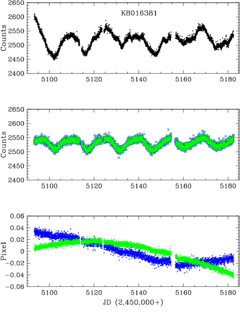
Figure 1b: The light curves for Kepler ID#5428432 as in Fig. 1. While our PCA analysis dramatically improved upon the pipeline processed light curve, it is impossible to discern which variations in the final light curve are due to intrinsic variability and which are due to the result of the sudden jumps in the location of the centroid of the star.

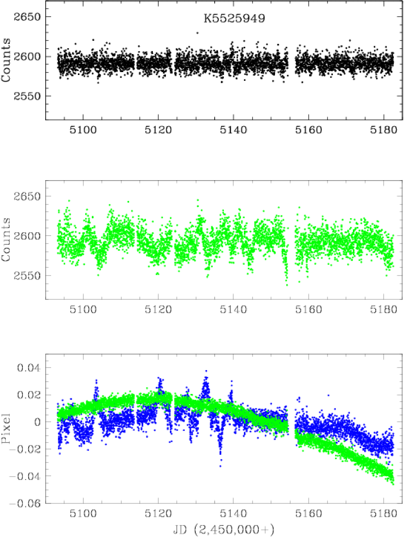
Figure 1c: The light curves for K5525949. In this case the $Kepler$ light curve reveals a non-variable source. The PCA light curve reveals an aperiodic variable due to “third light contamination” (the summed-pixel light curve has not been plotted so as to reduce clutter). As the object (or background source) brightened/dimmed, the centroid moved in the $-y$/$+y$ direction.

Figure 7: The derived rotation periods plotted vs. T_eff (black dots). The means in 200 K bins are plotted as green stars with error bars.

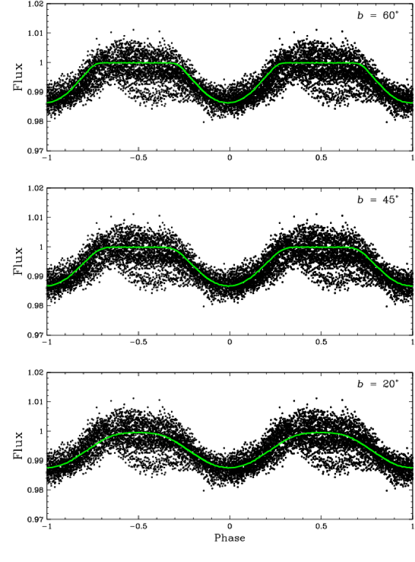
Figure 11a: The phased Q5 light curve of K10200948. Single spot models (green curves) with $i$ = 70^∘ are plotted in each panel. The co-latitude of the spot, $b$, is listed in top right corner of each panel.

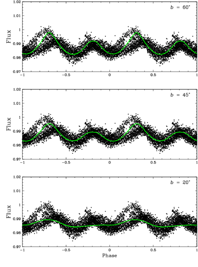
Figure 11b: The phased Q3 light curve of K10200948 as in Fig. 11a, but for two spot models.