Bayesian methods for genetic association analysis with heterogeneous subgroups: From meta-analyses to gene–environment interactions

Abstract

Genetic association analyses often involve data from multiple potentially-heterogeneous subgroups. The expected amount of heterogeneity can vary from modest (e.g., a typical meta-analysis) to large (e.g., a strong gene–environment interaction). However, existing statistical tools are limited in their ability to address such heterogeneity. Indeed, most genetic association meta-analyses use a “fixed effects” analysis, which assumes no heterogeneity. Here we develop and apply Bayesian association methods to address this problem. These methods are easy to apply (in the simplest case, requiring only a point estimate for the genetic effect and its standard error, from each subgroup) and effectively include standard frequentist meta-analysis methods, including the usual “fixed effects” analysis, as special cases. We apply these tools to two large genetic association studies: one a meta-analysis of genome-wide association studies from the Global Lipids consortium, and the second a cross-population analysis for expression quantitative trait loci (eQTLs). In the Global Lipids data we find, perhaps surprisingly, that effects are generally quite homogeneous across studies. In the eQTL study we find that eQTLs are generally shared among different continental groups, and discuss consequences of this for study design.

and T1Supported in part by NIH Grants HG02585 to M. Stephens and MH090951-02 (PI Jonathan Pritchard).

1 Introduction

We consider the following problem, which arises frequently in genetic association analysis: how to test for association while allowing for heterogeneity of effects among subgroups. We are motivated particularly by the following applications:

Motivating application 1: The Global Lipids genome-wide association study

The Global Lipids consortium [Teslovich et al. (2010)] conducted a large meta-analysis of genome-wide genetic association studies of blood lipids phenotypes [total cholesterol (TC), low-density lipoprotein cholesterol (LDL-C), high-density lipoprotein cholesterol (HDL-C) and triglycerides (TG)]. This study, like most meta-analyses, aimed to increase power by combining information across studies. The consortium amassed a total of more than 100,000 individuals, through 46 separate studies. These studies involve different investigators, at different centers, with different enrollment criteria. Consequently one would expect genetic effect sizes to differ among studies. However, Teslovich et al. (2010), following standard practice in this field, analyzed the data assuming no heterogeneity. This analysis appeared highly successful, identifying genetic associations at a total of 95 different genetic loci, 53 of them novel. Our work here was motivated by a desire to analyze these data, and others like them, taking account of potential heterogeneity among studies, and to see whether this would identify additional genetic associations.

Motivating application 2: Assessing heterogeneity of genetic effects on gene expression (eQTLs) among populations

An expression quantitative trait locus (eQTL) is a genetic variant that is associated with expression (activity) of a gene. Identifying eQTLs is important because such variants are candidates for being functional (i.e., actually causing changes in gene expression), and hence candidates for having other, perhaps medically important, consequences. See Gilad, Rifkin and Pritchard (2008) for more on insights to be gained from eQTL studies.

Here we analyze data from Stranger et al. (2007), who measured gene expression on lymphoblastoid cell lines derived from unrelated individuals sampled from three major continental groups: Europeans (CEU), Asians (ASN), and Africans (YRI). The main aim of our analysis is to assess heterogeneity of eQTL effects across groups: for example, do eQTL effects tend to vary among groups, and do some eQTLs appear to be active in only some groups? Understanding heterogeneity in this context could yield insights into differences in the gene-regulatory mechanisms acting in each group, and also has important implications for generalizability of studies performed in one subgroup to other subgroups. Similar questions also arise frequently in eQTL studies involving different tissue or cell types [Dimas et al. (2009), Brown, Mangravite and Engelhardt (2012), Flutre et al. (2013)].

Motivating application 3: Identifying biological interactions with environment

Our third example is more generic, but nonetheless important: identifying genetic associations in the presence of environmental interactions. Strong environmental interactions can result in genetic effects varying among subgroups, and in extreme cases could even cause effects to have different signs in different subgroups. In such cases ignoring heterogeneity would substantially reduce power. For example, by separately analyzing male and females, Kong et al. (2008) identified a strong genetic association with recombination rate that is missed by a standard analysis that ignores heterogeneity. However, separately analyzing subgroups is less attractive than analyzing them jointly and allowing for potential heterogeneity; this motivated development of methods described here.

These three applications differ in their expected heterogeneity. For example, whereas interactions could cause genetic effects to differ in sign among subgroups, differences in sign seem less likely in the meta-analysis setting. However, they also share an important element in common: the vast majority of genetic variants are unassociated with any given phenotype within all subgroups. Consequently, it is of considerable interest to identify genetic variants that show association in any subgroup or, in other words to reject the “global” null hypothesis of no association within any subgroup. This focus on rejecting the global null hypothesis distinguishes genetic association analyses from other settings and calls for analysis approaches tailored to this goal; see Lebrec, Stijnen and van Houwelingen (2010) for relevant discussion. Thus, although there has been previous work on Bayesian methods for meta-analysis [e.g., Sutton and Abrams (2001), Stangl and Berry (2000), DuMouchel and Harris (1983), Whitehead and Whitehead (1991), Li and Begg (1994), Eddy, Hasselblad and Schachter (1990), Givens, Smith and Tweedie (1997), Verzilli et al. (2008), De Iorio et al. (2011), Burgess et al. (2010), Mila and Ngugi (2011)], the nature of our applications calls for a different focus. Specifically, our applications need tools for association testing and model comparison, via Bayes Factors (BFs), rather than for estimation. In addition, because genetic association studies often involve very many association tests, computational speed is important, so we focus on obtaining fast numerical approximations to BFs (rather than using MCMC say). Finally, because in many cases, including the Global Lipids data above, only summary data (e.g., effect size estimates and standard errors in the different subgroups) are easily available, we need methods that can work with summary data.

Although our methods are Bayesian, they have close connections with related frequentist methods. Indeed, while this work was in progress, Lebrec, Stijnen and van Houwelingen (2010) [and, later, Han and Eskin (2011)] published frequentist approaches to association testing based on models very similar to those used here. Further, as we show in Section 4, some standard frequentist meta-analysis tests correspond closely to BFs obtained under certain priors. Consequently, ranking SNP associations by these standard test statistics is equivalent to making specific (and not necessarily realistic) prior assumptions. Thus, although our primary goal is to provide a practical solution to a common applied problem, we also provide theoretical results linking our methods to widely used existing methods.

2 Models and methods

The problems outlined above have two key goals:

1. To test whether a genetic variant is associated with phenotype in any subgroup, allowing for potential heterogeneity of effects among subgroups.

2. Given that an association exists, assess the support for different levels of heterogeneity.

We tackle these problems by specifying a family of alternative models with varying levels of heterogeneity, and by developing computational tools to calculate the support in the data (the BF) for each alternative model compared with the null model of no association. Within this framework the goal of testing the global null (1 above) is accomplished by assessing the overall support for any of the alternative hypotheses, whereas the goal of examining heterogeneity among groups is achieved by comparing the relative support for different alternative models.

All our motivating examples involve quantitative outcomes, and we focus on this case. However, in common to many meta-analysis methods, the simplest of our methods requires only an estimated effect size in each study and its corresponding standard deviation, and thus can be applied to any setting where such estimates are available (e.g., generalized linear models). See Appendix B of the supplementary material [Wen and Stephens (2014)] for details.

2.1 Notation and assumptions

Assume quantitative phenotype data and genotype data are available on $S$ predefined subgroups. Like most association analyses, we analyze each genetic variant in turn, one at a time. Assume that the data within subgroup $s$ come from $n_{s}$ randomly sampled unrelated individuals. Let the $n_{s}$-vectors $\mathbf{y}_{s}$ and $\mathbf{g}_{s}$ denote, respectively, the corresponding phenotype and genotype data, and $\mathbf{Y}:=(\mathbf{y}_{1},\ldots,\mathbf{y}_{S})$ and $\mathbf{G}:=(\mathbf{g}_{1},\ldots,\mathbf{g}_{S})$. Here each genotype is coded as 0, 1 or 2 copies of a reference allele, so $\mathbf{g}_{s}\in\{0,1,2\}^{n_{s}}$. (For imputed genotypes we replace each genotype with its posterior mean [Guan and Stephens (2008)], in which case $\mathbf{g}_{s}\in[0,2]^{n_{s}}$.)

2.2 Models for effect-size heterogeneity

Within each subgroup, we model genotype–phenotype association using a standard linear model:

$$\mathbf{y}_{s}=\mu_{s}{\mathbf{1}}+\beta_{s}\mathbf{g}_{s}+\mathbf{e}_{s},\qquad\mathbf{e}_{s}\sim\mathrm{N}\bigl{(}0,\sigma_{s}^{2}I\bigr{)}$$ (1)

with residual errors $\mathbf{e}_{s}$ assumed independent across subgroups. [Additional, possibly study-specific, covariates are easily added to the right-hand side of (1). If independent flat priors are used for the coefficients of these covariates within each study, then our main results below still hold, effectively unchanged. This treatment is analogous to the frequentist mixed-effects model, where such covariates are typically assumed to have study-specific effects.]

The “global” null hypothesis is no genotype–phenotype association within any subgroup, that is, $\beta_{s}=0$ for all $s$.

Under the alternative hypothesis the genetic effects are nonzero. To allow for heterogeneity among subgroups, we assume that these effects are normally distributed about some unknown common mean. We consider two different definitions of genetic effects: the “standardized effects”, $b_{s}:=\beta_{s}/\sigma_{s}$, and the unstandardized effects, $\beta_{s}$, leading to the following models:

[2.]

Exchangeable standardized effects (ES model). The standardized effects $b_{s}$ are normally distributed among subgroups, about some unknown mean $\bar{b}$, to which we assign a normal prior:

$$b_{s}|\bar{b},\sigma_{s} \sim \mathrm{N}\bigl{(}\bar{b},\phi^{2}\bigr{)}\quad\bigl{[}\mbox{or, equivalently, }\beta_{s}|\sigma_{s}\sim\mathrm{N}\bigl{(}\sigma_{s}\bar{b},\sigma_{s}^{2}\phi^{2}\bigr{)}\bigr{]},$$ (2)

$$\bar{b} \sim \mathrm{N}\bigl{(}0,\omega^{2}\bigr{)}.$$ (3)

Alternatively, and equivalently, the vector $\mathbf{b}=(b_{1},\ldots,b_{S})$ is multivariate normally distributed:

$$\mathbf{b}\sim\mathrm{N}_{S}(0,\Sigma_{b}),$$ (4)

where $\Sigma_{b}$ is an $S\times S$ matrix with diagonal elements $\operatorname{Var}(b_{s})=\phi^{2}+\omega^{2}$ and off-diagonal elements $\operatorname{Cov}(b_{s},b_{s^{\prime}})=\omega^{2}$.

Exchangeable effects (EE model). The unstandardized effects $\beta_{s}$ are normally distributed about some unknown mean $\bar{\beta}$, to which we assign a normal prior:

$$\beta_{s}|\bar{\beta} \sim \mathrm{N}\bigl{(}\bar{\beta},\psi^{2}\bigr{)},$$ (5)

$$\bar{\beta} \sim \mathrm{N}\bigl{(}0,w^{2}\bigr{)}.$$ (6)

Alternatively, and equivalently, the vector $\bolds{\beta}=(\beta_{1},\ldots,\beta_{S})$ is multivariate normally distributed:

$$\bolds{\beta}\sim\mathrm{N}_{S}(0,\Sigma_{\beta}),$$ (7)

where $\Sigma_{\beta}$ is an $S\times S$ matrix with diagonal elements $\operatorname{Var}(\beta_{s})=\psi^{2}+w^{2}$ and off-diagonal elements $\operatorname{Cov}(\beta_{s},\beta_{s^{\prime}})=w^{2}$.

In both ES and EE models we assume conjugate priors for $(\mu_{s},\sigma_{s})$:

$$\mathrm{ES}\dvtx\mu_{s}|\sigma_{s} \sim \mathrm{N}\bigl{(}0,\sigma_{s}^{2}u_{s}^{2}\bigr{)};\qquad\sigma_{s}^{-2}\sim\Gamma(m_{s}/2,l_{s}/2),$$ (8)

$$\mathrm{EE}\dvtx\mu_{s} \sim \mathrm{N}\bigl{(}0,u_{s}^{2}\bigr{)};\qquad\sigma_{s}^{-2}\sim\Gamma(m_{s}/2,l_{s}/2).$$ (9)

Specifically, we consider posteriors and BFs that arise in the limits $u_{s}^{2}\rightarrow\infty$ and $l_{s},m_{s}\rightarrow 0$. These limiting priors correspond to standard improper priors for normal regressions and ensure that the BFs satisfy certain invariance properties [see Servin and Stephens (2008)].

Both ES and EE have two key hyperparameters, one ($\omega$ in ES; $w$ in EE) that controls the prior expected size of the average effect across subgroups, and another ($\phi$ in ES; $\psi$ in EE) that controls the prior expected degree of heterogeneity among subgroups. A complimentary view is that $\omega^{2}+\phi^{2}$ (resp., $w^{2}+\psi^{2}$) controls the expected (marginal) effect size in each study and $\phi/\omega$ (resp., $\psi/w$) controls the degree of heterogeneity. Thus, one can allow for different levels of heterogeneity by considering different values of these hyperparameters (see below). Note that $\phi=0$ (resp., $\psi=0$) corresponds to the assumption, commonly used in practice, of no heterogeneity among subgroups.

Of the two models, ES has the advantage that it results in analyses (e.g., BFs) that are invariant to the phenotype measurement scale used within each subgroup. This makes it robust to users accidentally specifying phenotype measurements in different subgroups on different scales (a nontrivial issue in complex analyses involving collaboration among many research groups). It also makes it applicable when measurement scales are difficult to harmonize across subgroups, for example, due to use of different measurement technologies. For these reasons we prefer ES for general use. However, in some cases EE may be easier to apply. For example, if one has access only to published point estimates and standard errors for the effect size $\beta_{s}$ in each study, then this suffices to approximate the BF under EE, but not under ES. Note that ES and EE will produce similar results if the residual error variances are similar in all subgroups.

2.2.1 Limiting heterogeneity: A curved exponential family normal prior

The above priors assume independence of the mean ($\bar{b}$) and variance ($\omega^{2}$) of the effects. In some settings this assumption may be unattractive. For example, in a typical meta-analysis we expect effects to show “limited heterogeneity” across studies and typically to have the same sign [Owen (2009)], regardless of whether $\bar{b}$ is small or large. But the independence assumption implies that the probability that the effects have the same sign is much larger when $\bar{b}$ is large than when it is small. To address this, we can replace the priors (2) and (5) with, respectively,

$$b_{s} \sim \mathrm{N}\bigl{(}\bar{b},k^{2}{\bar{b}}^{2}\bigr{)},$$ (10)

$$\beta_{s} \sim \mathrm{N}\bigl{(}\bar{\beta},k^{2}{\bar{\beta}}{}^{2}\bigr{)}.$$ (11)

Here $k$ determines the amount of heterogeneity, with smaller $k$ indicating less heterogeneity and $k=0$ indicating no heterogeneity. Under these priors the probability of effects differing in sign depends only on $k$ and not on $\bar{b}$,

$$\Pr(b_{s}\mbox{ has a different sign from }\bar{b})=\Phi\biggl{(}-\frac{1}{|k|}\biggr{)},$$ (12)

where $\Phi$ is the cumulative distribution function of a standard normal distribution. For example, when $k=1/2$, (12) is approximately 2.3%.

We call these priors “Curved Exponential Family Normal” (CEFN) priors, reflecting their functional relationship between the mean and variance.

2.3 Bayes factors for testing the global null hypothesis

For simplicity we focus on calculations for the ES model; details for EE, and modifications for CEFN, are given in the appendices [supplementary material Wen and Stephens (2014)].

The ES model has two hyperparameters, $\phi$ and $\omega$. The global null hypothesis, which is most naturally written as $\beta_{s}\equiv 0$ for all $s$, can also be written as

$$H_{0}\dvtx\phi=\omega=0.$$ (13)

The support in the data for a particular alternative model, specified by hyperparameters $(\phi,\omega)$, vs $H_{0}$, is given by the Bayes Factor (BF):

$$\mathrm{BF}^{\mathrm{ES}}(\phi,\omega)=\frac{P(\mathbf{Y}|\mathbf{G},\phi,\omega)}{P(\mathbf{Y}|\mathbf{G},H_{0})}.$$ (14)

Each value of $(\omega,\phi)$ corresponds to a particular alternative model, with $\omega$ controlling the typical average effect size, and $\phi$ controlling the degree of heterogeneity among subgroups (or in a reparametrization, $\omega^{2}+\phi^{2}$ controls the expected marginal effect size in each subgroup and $\phi/\omega$ controls the degree of heterogeneity). To allow for uncertainty about appropriate values for $\phi$ and $\omega$, we use a (discrete) prior distribution on a set of plausible values $\{(\phi^{(i)},\omega^{(i)})\dvtx i=1,\ldots,M\}$ (see applications for details). (This induces a prior on the effects that is a mixture of multivariate normals.) A discrete prior is more flexible than fixing $\phi,\omega$ to specific values, while maintaining computational convenience. Indeed, if $\pi_{i}$ denotes the prior weight on $(\phi^{(i)},\omega^{(i)})$, then the resulting BF against $H_{0}$ is the weighted average of the individual BFs:

$$\mathrm{BF}^{\mathrm{ES}}_{\mathrm{av}}:=\sum_{i=1}^{M}\pi_{i}\mathrm{BF}^{\mathrm{ES}}\bigl{(}\phi^{(i)},\omega^{(i)}\bigr{)}.$$ (15)

This average could be extended to include other models (e.g., some using the CEFN prior, others not). The fact that BFs under different assumptions for heterogeneity can be both averaged in this way (to assess evidence against the global null, allowing for heterogeneity), and compared with one another (to assess the evidence for different levels or types of heterogeneity), is one nice feature of the Bayesian framework.

We make two comments regarding the need to specify the prior weights $\pi$ in (15). First, the usual practice of simply ignoring heterogeneity is implicitly making a particular, and rather strong, decision about $\pi$. In this sense, specifying weights for different amounts of heterogeneity is simply turning a usually implicit decision into an explicit decision. [See Wakefield (2009) for analogous discussion regarding choice of priors on effect sizes.] Second, in some applications it will be possible, and desirable, to learn these weights from the data via a hierarchical model, reducing the subjectivity of the analysis. Indeed, the ability of BFs to be naturally incorporated into a hierarchical model is one advantage over analogous frequentist test statistics [Lebrec, Stijnen and van Houwelingen (2010)] that maximize over $\phi,\omega$. This idea is illustrated in Section 3.3.

2.3.1 Calculating Bayes factors

Calculating $\mathrm{BF}^{\mathrm{ES}}(\phi,\omega)$ involves evaluating a multidimensional integral. In Appendix A of the supplementary material [Wen and Stephens (2014)] we present two different approximations, both based on applying Laplace’s method and both having error terms that decay inversely with the average sample size across subgroups. The first of these, which effectively follows methods from Butler and Wood (2002) for computing confluent hyper-geometric functions, is very accurate, even for small sample sizes. Indeed, for the special case of a single subgroup ($S=1$), the approximation becomes exact, and for small numbers of subgroups we have checked numerically (Appendix D of the supplementary material [Wen and Stephens (2014)]) that it provides almost identical results to an alternative approach based on adaptive quadrature (which is practical only for small $S$). However, it requires a numerical optimization step and has a somewhat complex form, which, although not a practical barrier to its use, does hinder intuitive interpretation. In what follows we use $\widehat{\mathrm{BF}}{}^{\mathrm{ES}}$ to denote this approximation.

The second approximation is less accurate for small samples sizes, but converges asymptotically (with average sample size) to the correct answer. Further, a simple modification, described in Appendix C of the supplementary material [Wen and Stephens (2014)], yields much greater accuracy. For the special case of $S=1$ it yields an analogue of the approximate BFs from Wakefield (2009) and Johnson (2008), and in what follows we use $\mathrm{ABF}^{\mathrm{ES}}$ to denote this approximation under the ES model. The nice feature of $\mathrm{ABF}^{\mathrm{ES}}$ is that it has an intuitive analytic form, which is detailed after the applications, in Section 4 (Proposition 4.1).

2.3.2 Special cases

Our ES and EE models include, in the special cases $\phi=0$ and $\psi=0$, the case where there is no heterogeneity of effects across subgroups. The assumption of no heterogeneity also underlies standard “fixed effects” meta-analysis methods, and so we use $\mathrm{ABF}_{\mathrm{fix}}^{\mathrm{ES}}$ and $\mathrm{ABF}_{\mathrm{fix}}^{\mathrm{EE}}$ to denote ABFs computed under these assumptions. These ABFs are the Bayesian analogues of standard frequentist test statistics for “fixed effect” analyses; see Section 4.2.1 for details.

At the other extreme, the cases $\omega=0$ (ES model) and $w=0$ (EE model) maximize heterogeneity across subgroups, and we use $\mathrm{ABF}_{\max\mathrm{H}}^{\mathrm{ES}}$, $\mathrm{ABF}_{\max\mathrm{H}}^{\mathrm{EE}}$ to denote ABFs computed under these assumptions. These ABFs can be viewed as the Bayesian analogues of frequentist methods that combine information across subgroups, ignoring the direction of the effect in each subgroup (e.g., Fisher’s method); see Section 4.2.2 for details.

2.3.3 Bayes factors from summary statistics

It turns out that both the true BFs ($\mathrm{BF}^{\mathrm{ES}}$, $\mathrm{BF}^{\mathrm{EE}}$) and the approximations $(\widehat{\mathrm{BF}}{}^{\mathrm{ES}}$, $\widehat{\mathrm{BF}}{}^{\mathrm{EE}}$, $\mathrm{ABF}^{\mathrm{ES}}$, $\mathrm{ABF}^{\mathrm{EE}})$ depend on the observed data in each subgroup only through a set of summary statistics, a 6-tuple $(n_{s},{\mathbf{1}}^{\prime}\mathbf{y}_{s},{\mathbf{1}}^{\prime}\mathbf{g}_{s},\mathbf{y}_{s}^{\prime}\mathbf{y}_{s},\mathbf{g}_{s}^{\prime}\mathbf{g}_{s},\mathbf{y}_{s}^{\prime}\mathbf{g}_{s})$. Furthermore, for the simplest approximations (the ABFs), the summary statistics needed from each subgroup are reduced to only $(\hat{b}_{s},\operatorname{se}(\hat{b}_{s}))$ for the ES model and ($\hat{\beta}_{s},\operatorname{se}(\hat{\beta}_{s}))$ for the EE model. These are exactly the quantities used in traditional meta-analysis applications.

These properties have important practical implications. First, they aid collaboration among groups, where sharing of raw data can be more difficult than sharing summary data. Second, and perhaps more importantly, it means that the methods, particularly the ABFs, are extremely flexible. Indeed, in any setting where an effect size estimate and its standard error can be obtained for each subgroup, these can be plugged in to compute an ABF. This can be viewed as an additional Laplace approximation (Appendix B of the supplementary material [Wen and Stephens (2014)]). Thus, the methods can easily handle study-specific covariates, and nonnormal data (e.g., using a generalized linear model within each subgroup).

2.3.4 Software

We implemented these methods in a software package MeSH (Meta-analysis with Subgroup Heterogeneity), available from http:// www.github.com/xqwen/mesh.

3 Applications

3.1 Illustrative example: deCODE recombination study

We first illustrate the methods on motivating application 3 where heterogeneity of effects is known to occur. The example involves three correlated genetic variants (SNPs) that were found, in a genetic association study of recombination rate by Kong et al. (2008), to be strongly associated with both male and female recombination rates, but with estimated effects in opposite directions (i.e., the allele associated with lower recombination rate in males is associated with higher recombination rate in females).

We applied our methods to these data, exploiting the ability to compute ABFs from summary data. Specifically, Table 1 of Kong et al. (2008) gives estimated effect sizes $\hat{\beta}_{\mathrm{male}}$ and $\hat{\beta}_{\mathrm{female}}$ for three relevant SNPs, as well as corresponding $p$-values, from which we infer approximate values for the standard errors $\operatorname{se}(\hat{\beta}_{\mathrm{male}})$ and $\operatorname{se}(\hat{\beta}_{\mathrm{male}})$. These summaries suffice to compute ABFs under the EE model. We treat males and females as two subgroups and consider 4 levels of expected marginal overall effect sizes with $\sqrt{\psi^{2}+w^{2}}=5,10,20,40$ (the phenotype scale being centi-Morgans) and 5 levels of heterogeneity with $\psi^{2}/w^{2}=0,0.5,1,2,\infty$. This yields a grid of $4\times 5$ different $(\psi,w)$ combinations, and we treat every grid value as a priori equally likely when computing $\mathrm{ABF}_{\mathrm{av}}^{\mathrm{EE}}$. (A denser grid could be used to obtain more precise estimates of $\psi$ and $w$, but this coarse grid suffices for our purposes here.)

Table 1: Bayesian analysis of genetic associations with recombination rate. The SNPs, estimated effect sizes and $p$-values are taken directly from Kong et al. (2008), Table 1. We compute approximate BFs under the EE model using these summary statistics. $\mathrm{ABF}^{\mathrm{EE}}_{\mathrm{single},\mathrm{male}}$ and $\mathrm{ABF}^{\mathrm{EE}}_{\mathrm{single},\mathrm{female}}$ are approximate BFs computed using only male subgroup and female subgroup data, respectively. $\mathrm{ABF}_{\mathrm{fix}}^{\mathrm{EE}}$ and $\mathrm{ABF}_{\mathrm{av}}^{\mathrm{EE}}$ are approximate BFs computed using both males and females jointly, either assuming no heterogeneity ($\mathrm{ABF}_{\mathrm{fix}}^{\mathrm{EE}}$) or averaging over a range of values of heterogeneity ($\mathrm{ABF}_{\mathrm{av}}^{\mathrm{EE}}$)

	Male		Female		Meta BFs
SNP	Effect ($\bolds{p}$-value)	$\mathbf{ABF^{EE}_{single,\,male}}$	Effect ($\bolds{p}$-value)	$\mathbf{ABF^{EE}_{single,\,female}}$	$\mathbf{ABF_{fix}^{EE}}$	$\mathbf{ABF_{av}^{EE}}$
rs3796619	$-$67.9 ($1.1\times 10^{-14}$)	0$10^{11.12}$	67.6 ($7.9\times 10^{-6}$)	$10^{2.81}$	$10^{3.07}$	$10^{13.91}$
rs1670533	$-$66.1 ($1.8\times 10^{-11}$)	$10^{8.06}$	92.8 ($4.1\times 10^{-8}$)	$10^{4.55}$	$10^{1.10}$	$10^{12.58}$
rs2045065	$-$66.2 ($1.6\times 10^{-11}$)	$10^{8.11}$	92.2 ($6.0\times 10^{-8}$)	$10^{4.40}$	$10^{1.18}$	$10^{12.49}$

The resulting BFs are shown in Table 1. Notably, the association signal in the joint analysis of males and females, allowing for heterogeneity, $\mathrm{ABF}_{\mathrm{av}}^{\mathrm{EE}}$, is many orders of magnitude larger than either of the subgroup-specific BFs, which are themselves larger than the BF under a fixed effects model, $\mathrm{ABF}_{\mathrm{fix}}^{\mathrm{EE}}$. This analysis illustrates two simple but important points. First, a joint analysis can yield a considerably stronger signal than subgroup-specific analyses. Second, a standard fixed-effects meta-analysis would be ineffective in this case. Of course, in general, the “right” level of heterogeneity is unknown; $\mathrm{ABF}_{\mathrm{av}}^{\mathrm{EE}}$ deals with this by averaging over different levels of heterogeneity. This ability to average over unknown quantities is an attractive feature of the Bayesian approach, although it can also be helpful to examine the components of this average separately (see the next application).

Our methods can also assess which associations show evidence for heterogeneity. This could help identify potentially interesting interactions (as in this case) or potentially suspect association signals (see next example). In these data $\mathrm{ABF}_{\mathrm{av}}^{\mathrm{EE}}$ is substantially larger than $\mathrm{ABF}_{\mathrm{fix}}^{\mathrm{EE}}$, indicating that the data are inconsistent with the fixed effects assumption of equal effects in both subgroups. This comparison is a Bayesian analogue of the frequentist test for heterogeneity in a random effects meta-analysis. To further investigate heterogeneity, we compare BFs for different values of the heterogeneity parameter ($\psi^{2}/w^{2}$); in this case the data are consistent with infinite values for this parameter (i.e., $w^{2}=0$).

This example illustrates that an association analysis accounting for heterogeneity can identify associations that would be missed by a fixed effects analysis that ignores heterogeneity. Next we attempt to exploit this to identify novel associations in a large-scale genome-wide association study.

3.2 Global Lipids genome-wide association study

We now return to motivating application 1, a large scale meta-analysis of genome-wide genetic association studies of blood lipids phenotypes conducted by the Global Lipids consortium [Teslovich et al. (2010)]. In this study, more than 100,000 individuals of European ancestry were amassed through 46 separate studies (grouped into 25 studies in their final analysis). For each individual, measures of total cholesterol (TC), low-density lipoprotein cholesterol (LDL-C), high-density lipoprotein cholesterol (HDL-C) and triglycerides (TG) were obtained. Genotypes at 2.7 million SNPs across the genome were also measured or imputed. In each study, the phenotypes were independently quantile normal transformed; single SNP association tests were performed for all SNPs and all phenotypes using the linear model (1) and estimated effects and their standard errors were computed. The meta-analysis combined these summary data using the software METAL [Willer, Li and Abecasis (2010)] to compute a weighted $Z$ statistic that we discuss later [specifically they used equation (26) with weights $w_{s}=\sqrt{n_{s}}$]. This can be viewed as an approximation to a fixed effects analysis under the ES model (see Section 4.2.1). Teslovich et al. (2010) reported 168 SNP-phenotype associations exceeding their “genome-wide significant” threshold ($p$-value $<5\times 10^{-8}$) and identified 95 genes, with 59 showing genome-wide significant association for the first time.

We hypothesized that taking account of heterogeneity among subgroups might help identify additional novel associations, so we reanalyzed the data using our Bayesian tools to allow for heterogeneity. We were able to obtain access to summary data from each study, in the form of an estimated effect size (computed from the quantile-transformed phenotype data) and its standard error for each SNP in each study. With these data we can perform analyses under the EE model for the quantile normalized data (rather than the ES model effectively used in the original analysis). We computed ABFs under increasing amounts of heterogeneity: the fixed effects model, the “limited heterogeneity” CEFN model, and the maximum heterogeneity model. In each case we assumed a discrete uniform prior on the overall genetic effect size [i.e., $(k^{2}+1)w^{2}$ in the CEFN model and $w^{2}+\psi^{2}$ in the other models] on the set $\{0.1^{2},0.2^{2},0.4^{2},0.6^{2},0.8^{2}\}$. For the fixed effects model, $\psi=0$; for the maximum heterogeneity model, $w=0$; and for the CEFN model, we set $k=0.326$, which gives a prior probability of $1/1000$ that the genetic effect in each study has an opposite sign to $\bar{\beta}$. Although a fully automated Bayesian analysis would naturally average over the different models for heterogeneity, in practice, because of their different sensitivity to particular data features (see below), we found it helpful to examine each separately.

As an initial check on data handling we verified that our Bayesian fixed effects analysis produced similar results to the original fixed effects analysis. As expected, we found that $\mathrm{ABF}_{\mathrm{fix}}^{\mathrm{EE}}$ ranked SNP associations very similarly to the original reported (ES model) $p$-values. However, there were some notable exceptions. In particular, a few SNPs showed a much stronger association signal in $\mathrm{ABF}_{\mathrm{fix}}^{\mathrm{EE}}$ than the original analysis. Further investigation suggested that these results likely reflected the EE analysis being less robust to data processing errors than the original ES analysis. For example, SNP rs17061870 with LDL phenoype had a huge signal in our EE analysis ($\mathrm{ABF}_{\mathrm{fix}}^{\mathrm{EE}}>10^{17}$) and a very modest signal in the original analysis ($p$-value${}=0.028$), but examination of the study-specific data for this SNP showed a suspicious pattern: the $p$-value was $2\times 10^{-31}$ in one study (the Family Heart Study, FHS), but no smaller than 0.1 in the 5 other studies for which this SNP had genotype data available. Furthermore, the very small $p$-value in FHS was driven primarily by a very small, probably erroneous, estimate of the residual error in that study (the sample size of this particular study is not large) which under the EE model results in a very high weight on that study, but in the ES model does not (see Section 4.2.1). We emphasize that we performed the EE analysis here because it was what we were able to do easily with the available summary data, rather than because we prefer it.

Next we assessed evidence for heterogeneity of effects in the 168 association signals reported by the original analysis. We did this by comparing the support for the limited heterogeneity model ($\mathrm{ABF^{EE}_{cefn}}$) with the support for the no heterogeneity model ($\mathrm{ABF^{EE}_{fix}}$). The majority of phenotype-SNP pairs ($111/168$) showed stronger support for the no heterogeneity model (Figure 1). This result was surprising to us: this meta-analysis involved a large number of different studies, encompassing a range of different enrollment criteria, so we expected to find much stronger evidence for heterogeneity among studies. We did find three strong associations that showed overwhelming support for heterogeneity ($\mathrm{ABF^{EE}_{cefn}}/\mathrm{ABF^{EE}_{fix}}>10^{10}$; Figure 1). Forest plots for these SNPs (Figure 2) suggest that in all three cases this signal for heterogeneity comes from modest variation in effect size among all studies, rather than a strong difference in one or a few studies (although the B58C-WTCCC study is, arguably, something of an outlier at rs3764261).

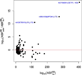
Figure 1: Assessment of evidence for heterogeneity in 168 reported phenotype-SNP association signals from Teslovich et al. (2010). Large values on the $y$ axis indicate stronger support for the model, allowing for limited heterogeneity ($\mathrm{ABF^{EE}_{cefn}}$) compared with the model with no heterogeneity ($\mathrm{ABF^{EE}_{fix}}$). The three highlighted points correspond to associations with overwhelming evidence for heterogeneity, $\mathrm{ABF^{EE}_{cefn}}/\mathrm{ABF^{EE}_{fix}}>10^{10}$; forest plots for these are shown in Figure 2.

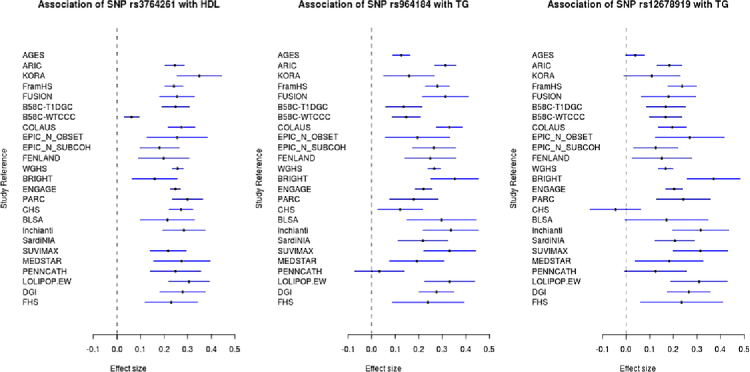
Figure 2: Forest plots for the three highlighted association signals in Figure 1, which showed overwhelming evidence for heterogeneity of (apparent) effects.

Finally, we addressed the primary question of interest: whether allowing for heterogeneity across studies yields novel associations. To do this, we performed a genome-wide analysis for each phenotype, in each case excluding all SNPs within 1 Mb of any SNPs originally reported as associated with that phenotype. We searched for SNPs that showed strong evidence for association under one of the heterogeneity models ($\mathrm{ABF^{EE}_{cefn}}$ or $\mathrm{ABF}_{\max\mathrm{H}}^{\mathrm{EE}}\geq 10^{6}$, where $\mathrm{ABF_{\max\mathrm{H}}^{EE}}$ denotes the approximate Bayes factor computed by restricting $w=0$, see Section 4.2.2 for precise definition) but not under the fixed-effects model ($\mathrm{ABF^{EE}_{fix}}<10^{6}$). This threshold ($10^{6}$) corresponds very roughly to, and is perhaps slightly more conservative than, the threshold effectively used in the initial analysis. (We used the same threshold for all three models for simplicity, but different thresholds might be more appropriate; for example, one might prefer a more stringent threshold for $\mathrm{ABF_{\max\mathrm{H}}^{EE}}$ because strong heterogeneity is unexpected in this context.)

Table 2: Association signals that show strong association under the models allowing for heterogenetiy ($\mathrm{ABF^{EE}_{cefn}}$ or $\mathrm{ABF_{\max\mathrm{H}}^{EE}}\geq 10^{6}$) but less strong under a model with no heterogeneity ($\mathrm{ABF^{EE}_{fix}}<10^{6}$). It seems likely that the last two of these represent false positive associations, but we include them in the table for completeness (see text for discussion)

Phenotype	SNP	Gene region	$\bolds{\log}_{\mathbf{10}}\bolds{(}\mathbf{BF^{EE}_{fix}}\bolds{)}$	$\bolds{\log}_{\mathbf{10}}\bolds{(}\mathbf{BF}^{\mathbf{EE}}_{\bolds{\max}\,\mathbf{H}}\bolds{)}$	$\bolds{\log}_{\mathbf{10}}\bolds{(}\mathbf{BF^{EE}_{cefn}}\bolds{)}$
LDL	rs1800978	5’UTR of ABCA1	$5.2$	$3.4$	6.0
TG	rs1562398	Flanking KLF14	$5.3$	$-0.2$	6.5
HDL	rs11229165	Flanking OR4A16	$4.6$	$4.9$	6.4
HDL	rs7108164	Flanking OR4A42P	$4.2$	$4.9$	6.3
HDL	rs11984900	N.A.	$-1.1$	$16.6$	6.2
HDL	rs6995137	Flanking SFRP1	$-0.4$	$6.9$	4.8

Overall we found 42 SNP-phenotype associations satisfying this criteria (after removing SNPs in LD with one another), representing associations potentially missed by the original analysis. However, detailed investigation suggested that 36 of these were not genuine associations. Specifically, these 36 associations, which showed strong signals in $\mathrm{ABF_{\max\mathrm{H}}^{EE}}$ only, were driven by strong associations in the FHS study that are likely due to data processing errors (the FHS $p$-values at these SNPs for quantile transformed phenotypes were many orders of magnitude smaller than for the original phenotypes). We therefore dropped the FHS data and re-performed the association analysis.

After dropping FHS, all 6 remaining signals from the previous analysis still satisfy our association criteria (Table 2). Of those, the first two listed are almost certainly genuine: the genes ABCA1 and KLF14 are reported in Teslovich et al. (2010) as associated with other lipid phenotypes (ABCA1 with HDL and TC; KLF14 with HDL), but not with the phenotypes we listed in Table 2, and both reflect associations that just missed being significant in the original fixed effects analysis. The next two associations may also be real: they map approximately 6 Mb apart on chromosome 11, in a region that is densely populated with olfactory receptor genes, and this same genetic region is also identified in a multivariate association analysis of these same data [Stephens (2013)], although we know of no further independent evidence to support them. One slight cause for caution is that, in humans, SNPs this far apart would usually not be correlated with one another, but these two are slightly correlated ($r^{2}\approx 0.07$ in the European 1000 Genomes data), raising the possibility of mapping errors. That is, the precise locations of these SNPs may be in question, and certainly it is difficult to say which genes they might implicate; the table simply lists the nearest gene for reference. Finally, based on examination of the raw data, we suspect that the last two associations are false positives, driven by apparent anomalies in a single study (this time B58C-WTCCC).

In summary, we find that the original fixed effects analysis in Teslovich et al. (2010) was highly effective. This may seem surprising, since these data seem to provide ample opportunities for heterogeneity of effects. Indeed, some of the associations identified by the original study do show a substantially stronger signal in analyses allowing for heterogeneity (Figure 1), and a genome-wide association analysis allowing for heterogeneity identified at least two apparently real associations that just missed being significant under the original fixed effects analysis. Thus, despite the success of the fixed effects analysis, analyses allowing for heterogeneity could modestly increase in power for GWAS meta-analyses in general. On the other hand, our results also provide a cautionary tale: in the context of meta-analysis of genetic association studies, when associations appear only under models allowing for strong heterogeneity, and not under fixed effects models, the reasons for the discrepancy must be examined carefully and the results interpreted critically. Indeed, we found that searching for SNPs showing strong heterogeneity is an effective way to identify data processing errors that may otherwise lurk undetected!

3.3 Heterogeneity of eQTLs among populations

Now we consider our second motivating application, examining heterogeneity in the effects of expression quantitative trait loci (eQTLs) among populations. An eQTL is a genetic variant (here, a SNP) that is associated with gene expression. Understanding heterogeneity of eQTL effects among population subgroups is important for several reasons. For example, it is important for designing and interpreting experiments, because it influences how generalizable results obtained in one subgroup are to other subgroups. In addition, identifying heterogeneous effects could yield insights into biological differences among subgroups: if an eQTL is more active in one subgroup than others, it may indicate a difference in the regulatory mechanisms operating in that subgroup.

To assess heterogeneity of eQTLs among European, African and Asian subgroups, we analyzed gene expression measurements from Stranger et al. (2007), obtained using the Illumina Sentrix Human-6 Expression BeadChip, on lymphoblastoid cell lines. Specifically, we considered the subset of 141 cell lines [41 Europeans (CEU), 59 Asians (ASN) and 41 Africans (YRI)] that were fully sequenced in the pilot project of the 1000 Genomes project [Durbin et al. (2010)]. We analyzed the 8427 distinct autosomal genes that were confirmed to be expressed in the same African samples by an independent experiment [Pickrell et al. (2010)]. We used SNP genotype data on 14.4 million SNPs from the final release (March, 2010) of the pilot SNP calls from the 1000 genomes project, with no additional allele frequency filtering. In addition to the original normalization Stranger et al. (2007), we performed quantile normal transformations to expression values for each gene, separately within each population group, to reduce the influence of outliers or other deviations from normality. Previous studies have shown that most eQTLs are located near to the gene whose expression they influence (so-called “cis-eQTLs”). Therefore, for each gene we restricted our association analysis to the “cis SNPs” which lie within the region 500 kb upstream of the transcription start site and 500 kb downstream of the transcription end site.

=205pt $\bolds{\phi^{2}/\omega^{2}}$ Posterior mean 95% credible interval 0 0.700 (0.640, 0.753) $1/4$ 0.265 (0.195, 0.330) $1/2$ 0.015 (0.002, 0.052) 1 0.008 (0.003, 0.016) $2/1$ 0.007 (0.002, 0.015) $4/1$ 0.004 (0.001, 0.012) $\infty$ 0.003 (0.000, 0.010)

Table 3: Estimated heterogeneity of eQTL effects among Europeans, Africans and Asians, obtained by fitting a hierarchical model to combine information across genes

Our analysis focuses on the question: how much do eQTL effects vary among continental groups? To assess this, we applied the ES model with $\sqrt{\phi^{2}+\omega^{2}}\in\{0.1,0.2,0.4,0.8,1.6\}$ and $\phi^{2}/\omega^{2}\in\{0,1/4,1/2,1,2,4,\infty\}$, producing a total grid of 35 different $(\phi,\omega)$ combinations. These values were chosen to cover a wide range of possible effect sizes and levels of heterogeneity. Since the amount of heterogeneity is our main interest, we estimate the weights $(\pi)$ on the 35 combinations using a Bayesian hierarchical model that jointly analyzes all 8427 genes. In brief, this model assumes the following: (i) the data at each gene are independent; (ii) each gene has at most one eQTL, with each SNP being equally likely; and (iii) that each eQTL draws its $(\phi,\omega)$ value from the grid of 35 different values, according to $\pi$. In addition, we assign a uniform prior to $\pi$. Under these assumptions, we implement a Markov Chain Monte Carlo (MCMC) algorithm to perform posterior inference on $\pi$. [See Wen (2011), Flutre et al. (2013) for full details of the computational methods and modeling assumptions.]

The results (Table 3) suggest that eQTL effects typically vary little among subgroups: the estimates from the hierarchical model put 97% of the total weight on the two smallest heterogeneity parameters, 0 and $1/4$. (For completeness we also include estimated grid weights on $\phi^{2}+\omega^{2}$, which control the average eQTL effect sizes, in Table 4.)

=205pt $\bolds{\sqrt{\omega^{2}+\phi^{2}}}$ Posterior mean 95% credible interval 0.1 0.004 (0.001, 0.008) 0.2 0.004 (0.001, 0.007) 0.4 0.008 (0.003, 0.014) 0.8 0.976 (0.966, 0.983) 1.6 0.007 (0.002, 0.015)

Table 4: Estimated standard deviation of average eQTL effects ($\sqrt{\omega^{2}+\phi^{2}}$), obtained by fitting a hierarchical model to combine information across genes

The above analysis effectively assumes that each eQTL is active in all three populations and allows for heterogeneity by allowing that the effect size may vary among populations. That is, it is effectively a model for “quantitative heterogeneity”. A different model for heterogeneity is that some eQTLs may be active in only a subset of the populations, with no effect in others, that is, that heterogeneity might be qualitative, with some eQTLs being “population-specific”. Although our quantitative-heterogeneity analysis above suggests that heterogeneity is generally low, it does not preclude the existence of some population-specific effects, so we performed an additional analysis to assess how common such population-specific effects might be. To apply our methods to this situation, we introduce $C$ to denote a binary string of indicators for whether an eQTL is active (i.e., has nonzero effect) in each population. For example, $C=(110)$ would indicate that the eQTL is active only in the first two populations. For the three populations in our data, $C$ has $2^{3}$ possible values, which we refer to as “configurations”. The support (BF) for each configuration, relative to the null model $C=(000)$, is easily computed. For example, for $C=(110)$,

$$\mathrm{BF}_{C=(110)} = \frac{P(\mathbf{y}_{1},\mathbf{y}_{2},\mathbf{y}_{3}|\mathbf{g}_{1},\mathbf{g}_{2},\mathbf{g}_{3},C=(110))}{P(\mathbf{y}_{1},\mathbf{y}_{2},\mathbf{y}_{3}|\mathbf{g}_{1},\mathbf{g}_{2},\mathbf{g}_{3},C=(000))}$$

$$= \frac{P(\mathbf{y}_{1},\mathbf{y}_{2}|\mathbf{g}_{1},\mathbf{g}_{2})}{P(\mathbf{y}_{1},\mathbf{y}_{2}|H_{0})}.$$

[The simplification is due to the assumption that the vectors of residual errors in (1) are independent across populations.]

Table 5: Estimated proportion of eQTLs that are shared among the three continental subgroups, represented by CEU (European), ASN (Asian) and YRI (African) samples. Estimates come from fitting a hierarchical model to combine information across genes; see text. The vast majority of eQTLs are estimates to be shared among all three subgroups

Configuration	Estimate (posterior mean)	95% credible interval
CEU only	0.001	(0.000, 0.003)
ASN only	0.001	(0.000, 0.008)
YRI only	0.001	(0.000, 0.004)
CEU and YRI	0.001	(0.000, 0.013)
ASN and YRI	0.017	(0.010, 0.035)
CEU and ASN	0.026	(0.014, 0.041)
CEU and ASN and YRI	0.953	(0.934, 0.970)

To estimate the proportion of eQTLs that follow each (nonnull) configuration, we introduce hyperparameters, $\eta_{001},\ldots,\eta_{111}$, to represent the frequency of each nonnull configuration. So each eQTL draws its configuration $C$ independently according to $\eta$. Furthermore, given $C$, we assume the standardized eQTL effect sizes follow the CEFN prior with $k=0.314$ and $\omega$ drawn independently from a grid $\{0.1,0.2,0.4,0.8,1.6\}$ according to weights $\pi^{\prime}$. Putting this all together into a single hierarchical model, with uniform priors on $\pi^{\prime}$ and $\eta$, we use MCMC to sample from the joint posterior distribution on all parameters. Full details are given in Wen (2011), Flutre et al. (2013).

The resulting estimates for $\eta$ are given in Table 5. Consistent with the conclusions on low overall heterogeneity above, the vast majority of eQTLs behave consistently across populations: indeed, we estimate $95\%$ of eQTLs to be active in all three populations. Nonetheless, we find some evidence for occasional deviations from this pattern, with approximately $2\%$ of eQTLs being active only in European and Asian samples, and $2\%$ being active only in Asian and African. Illustrative examples of potential exceptions to the general rule of sharing among populations are shown in Figures 3 and 4.

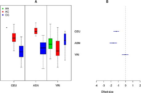
Figure 3: Example of a potential population specific eQTL presented only in CEU and ASN. A: Boxplots of the gene expression levels of gene CMAH (Ensemble ID ENSG00000168405) according to genotypes of SNP rs6906102 in the three Hapmap populations. B: forest plot of estimated effect sizes of this eQTL. Allele A of this SNP has allele frequencies 0.22, 0.08 and 0.67 in ASN, CEU and YRI, respectively.

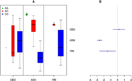
Figure 4: Example of a potential population specific eQTL presented only in ASN and YRI. A: Boxplots of the gene expression levels of gene PAQR8 (Ensemble IDENSG00000170915) according to genotypes of SNP rs3180068 in the three Hapmap populations. B: forest plot of estimated effect sizes of this eQTL. Allele A of this SNP has sample allele frequencies 0.14, 0.22 and 0.07 in ASN, CEU and YRI, respectively.

4 Analytic expressions for the Bayes factors and connections with frequentist statistics

We now provide analytic expressions for the ABFs mentioned above (Proposition 4.1 below). These expressions provide intuitive insights and highlight connections with standard frequentist test statistics, effectively establishing the “implicit prior assumptions” underlying some standard frequentist procedures. We start by introducing necessary notation:

• Association testing in a single subgroup. Consider analyzing a single subgroup, $s$. Let $\hat{\beta}_{s}$ and $\hat{\sigma}_{s}$ denote the least square estimates of $\beta_{s}$ and $\sigma_{s}$ from the linear regression model (1) using only data from subgroup $s$. The following expressions give an estimate for the standardized effect $b_{s}$ ($\hat{b}_{s}$), its standard error under $H_{0}$ ($\delta_{s}$) and a $t$-statistic for testing $b_{s}=0$ ($T_{s}$):

  $$\hat{b}_{s} := \hat{\beta}_{s}/\hat{\sigma}_{s},$$ (17)

  $$\delta^{2}_{s} := \frac{1}{\mathbf{g}_{s}^{\prime}\mathbf{g}_{s}-n_{s}\bar{g}_{s}^{2}},$$ (18)

  $$T_{s}^{2} := \frac{\hat{b}_{s}^{2}}{\operatorname{se}(\hat{b}_{s})^{2}}=\frac{\hat{\beta}_{s}^{2}}{\hat{\sigma}_{s}^{2}\delta_{s}^{2}}.$$ (19)

  Note that $T_{s}$ is also equal to $\hat{\beta}_{s}/\operatorname{se}(\hat{\beta}_{s})$, which is the usual t-statistic for testing $\beta_{s}=0$.

  Both Wakefield (2009) and Johnson (2008) derive the following approximate BF for testing $b_{s}\sim\mathrm{N}(0,\phi^{2})$ vs. $b_{s}=0$:

  $$\mathrm{ABF_{single}^{ES}}(T_{s},\delta_{s};\phi):=\sqrt{\frac{\delta_{s}^{2}}{\delta_{s}^{2}+\phi^{2}}}\exp\biggl{(}\frac{T_{s}^{2}}{2}\frac{\phi^{2}}{\delta^{2}_{s}+\phi^{2}}\biggr{)}.$$ (20)

  As noted by Wakefield, if $\phi$ is chosen differently for each SNP, and proportional to the value of $\delta^{2}_{s}$ for that SNP, then $\mathrm{ABF_{single}^{ES}}$ ranks the SNPs in the same way as the usual test statistic $T_{s}$. This result connects the standard frequentist analysis to a particular (approximate) Bayesian analysis in the case of a single subgroup. Proposition 4.1 below extends this to multiple subgroups, allowing for heterogeneity among subgroups.

• Testing average effect in a random effect meta-analysis model. Consider the standard frequentist test of $\bar{b}=0$ in a random effect meta-analysis of all subgroups, with $b_{s}\sim\mathrm{N}(\bar{b},\phi^{2})$. If $\phi$ is considered known, then an estimate for $\bar{b}$, its standard error $\zeta$ and a test statistic $\mathcal{T}_{\mathrm{ES}}^{2}$ for testing $\bar{b}=0$ are given by

  $$\hat{\bar{b}} := \frac{\sum_{s}(\delta_{s}^{2}+\phi^{2})^{-1}\hat{b}_{s}}{\sum_{s}(\delta_{s}^{2}+\phi^{2})^{-1}},$$ (21)

  $$\zeta^{2} := \frac{1}{\sum_{s}(\delta_{s}^{2}+\phi^{2})^{-1}},$$ (22)

  $$\mathcal{T}_{\mathrm{ES}}^{2} := \frac{\hat{\bar{b}}^{2}}{\operatorname{se}(\hat{\bar{b}})^{2}}.$$ (23)

  Applying Johnson’s idea [Johnson (2005, 2008)], we can “translate” this test statistic into an approximate BF for testing $\bar{b}\sim\mathrm{N}(0,\omega^{2})$ vs. $\bar{b}=0$, which yields

  $$\mathrm{ABF_{single}^{ES}}\bigl{(}\mathcal{T}_{\mathrm{ES}}^{2},\zeta;\omega\bigr{)}:=\sqrt{\frac{\zeta^{2}}{\zeta^{2}+\omega^{2}}}\exp\biggl{(}\frac{\mathcal{T}_{\mathrm{ES}}^{2}}{2}\frac{\omega^{2}}{\zeta^{2}+\omega^{2}}\biggr{)}.$$ (24)

Now $\mathrm{ABF}^{\mathrm{ES}}(\phi,\omega)$ can be written as a simple product of the ABFs (20) and (24).

Proposition 4.1

Under the ES model, applying a version of Laplace’s method to approximate $\mathrm{BF^{ES}}(\phi,\omega)$ yields the approximation

$$\mathrm{BF^{ES}}(\phi,\omega) \approx \mathrm{ABF}^{\mathrm{ES}}(\phi,\omega)$$

$$:= \mathrm{ABF_{single}^{ES}}\bigl{(}\mathcal{T}_{\mathrm{ES}}^{2},\zeta;\omega\bigr{)}\cdot\prod_{s}\mathrm{ABF_{single}^{ES}}\bigl{(}T_{s}^{2},\delta_{s};\phi\bigr{)}$$

and $\mathrm{ABF}^{\mathrm{ES}}(\phi,\omega)$ converges (almost surely) to $\mathrm{BF^{ES}}(\phi,\omega)$ as $n_{s}\to\infty$ for all subgroups $s$.

See Appendix A.1 of the supplementary material [Wen and Stephens (2014)].

Note 4.1

If the study-specific residual error variances, $\sigma_{s}$, are considered known (rather than being assigned a prior distribution) and used in place of $\hat{\sigma}_{s}$ to compute $\mathrm{ABF}^{\mathrm{ES}}$, then the approximation is exact, and $\mathrm{ABF}^{\mathrm{ES}}(\phi,\omega)=\mathrm{BF^{ES}}(\phi,\omega)$. This fact, together with the fact that the estimators $\hat{\sigma}_{s}$ are consistent for $\sigma_{s}$, explains, intuitively, why the proposition holds.

Note 4.2

The numerical accuracy of $\mathrm{ABF}^{\mathrm{ES}}$ as an approximation to $\mathrm{BF^{ES}}$ depends on sample sizes, and for small sample sizes it may be too inaccurate for routine application. However, a simple modification, described in Appendix C of the supplementary material [Wen and Stephens (2014)], yields much greater accuracy.

Proposition 4.1 partitions the evidence for association into two parts: one part reflects the evidence in each subgroup (the second term) and the other reflects consistency of effects among subgroups (the first term). In particular, if all subgroups show effects in the same direction, then the first term may be large ($\gg 1$) and “boost” the evidence for association. A similar result holds for the EE model (Appendix A.2 of the supplementary material [Wen and Stephens (2014)]).

4.1 Properties of Bayes factors

4.1.1 Induced single study Bayes factors

For the ES model, in the special case of one subgroup ($S=1$), both the actual BF and our approximations reduce to results from previous work. Specifically, the approximation $\widehat{\mathrm{BF}}{}^{\mathrm{ES}}$ becomes exact in this case, and equal to the BF derived by Servin and Stephens (2008), whereas $\mathrm{ABF}^{\mathrm{ES}}$ is equal to the ABF in Wakefield (2009) [see also Johnson (2005, 2008)].

4.1.2 Noninformative subgroup data

Suppose that in one subgroup, $s$, sample genotypes vary very little. This might arise, for example, in cross-population genetic studies, if one SNP allele is very rare in one population. Intuitively, subgroup $s$ then contains little information for testing $H_{0}$. Indeed, this will be reflected in the standard error for the effect size, $\delta_{s}$, being large, which will result in study $s$ contributing little to the BF. Specifically, in the limit $\delta_{s}\rightarrow\infty$, the ABF (4.1) is unaffected by the association data in study $s$ ($T_{s}$); a similar result holds for the exact BF (Appendix A of the supplementary material [Wen and Stephens (2014)]) and for both EE and ES. Thus, the BF correctly reflects the noninformativeness of the data from study $s$. Although one might expect every reasonable statistical procedure to possess this very intuitive property, many widely used methods do not (e.g., Fisher’s combined probability test).

4.2 Extreme models and connections with frequentist tests

The proposed models are very flexible, covering a wide range of types and degrees of heterogeneity by setting different values for $(\phi,\omega)$ (or $k$ in the CEFN prior). Here we discuss the two extremes of no heterogeneity (“fixed effects”) and maximum heterogeneity, and establish connections with frequentist testing approaches in these settings.

4.2.1 The fixed effects model

The fixed effects model assumes genetic effects to be homogeneous across subgroups, and corresponds to $\phi=0$ in ES or $\psi=0$ in EE. In these cases the test statistics $\mathcal{T}_{\mathrm{ES}}$ and $\mathcal{T}_{\mathrm{EE}}$ have particularly simple forms, being a weighted sum of individual $T_{s}$ statistics from each study (often referred to as a weighted sum of $Z$ scores when sample sizes are large). Specifically,

$$\mathcal{T}=\frac{\sum_{s}w_{s}T_{s}}{\sqrt{\sum_{s^{\prime}}w_{s^{\prime}}^{2}}},$$ (26)

where,

1. [2.]

2. For the ES model, $w_{s}=\operatorname{se}(\hat{b}_{s})^{-1}\approx\sqrt{2n_{s}f_{s}(1-f_{s})}$,

3. For the EE model, $w_{s}=\operatorname{se}(\hat{\beta}_{s})^{-1}\approx\hat{\sigma}_{s}^{-1}\sqrt{2n_{s}f_{s}(1-f_{s})}$,

and $f_{s}$ denotes the allele frequency of the target SNP in subgroup $s$. (The approximations come from assuming Hardy–Weinberg equilibrium in each subgroup.) These representations clarify a key practical difference between the ES and EE models: EE upweights studies with small residual error variance. Note also that $T_{s}$ is the same for both EE and ES, and independent of measurement scale, but $\sigma_{s}$ depends on measurement scale, so $\mathcal{T}_{\mathrm{ES}}$ is robust to studies using different measurement scales (or different transformations of the phenotypes) but $\mathcal{T}_{\mathrm{EE}}$ is not. In addition, these representations clarify the connection between these statistics and the methods used in the meta-analysis software METAL [Willer, Li and Abecasis (2010)]. Specifically, METAL implements tests using the weighted statistic (26) with two different weighting schemes, one corresponding to the EE model weights above and the other with the weights equal to $\sqrt{n_{s}}$. This latter scheme corresponds to the ES model only if $f_{s}$ is equal across studies. [Where $f_{s}$ varies across studies the weighting in the ES model seems, to us, preferable to the METAL scheme since studies with small $f_{s}(1-f_{s})$ provide less information.]

Returning now to the BFs, when $\phi=0$ the ABF (4.1) simplifies to

$$\qquad\mathrm{ABF}_{\mathrm{fix}}^{\mathrm{ES}}(\omega):=\mathrm{ABF^{ES}}(\phi=0,\omega)=\sqrt{\frac{\zeta^{2}}{\zeta^{2}+\omega^{2}}}\cdot\exp\biggl{(}\frac{\mathcal{T}_{\mathrm{ES}}^{2}}{2}\frac{\omega^{2}}{\zeta^{2}+\omega^{2}}\biggr{)},$$ (27)

where

$$\zeta^{2}=\frac{1}{\sum_{s}\delta_{s}^{-2}}.$$ (28)

A similar expression holds for $\mathrm{ABF^{EE}_{fix}}(w):=\mathrm{ABF^{EE}}(\psi=0,w)$.

We now answer the following question: under what prior assumptions will $\mathrm{ABF}_{\mathrm{fix}}^{\mathrm{ES}}$ produce the same SNP rankings as the frequentist test statistic $\mathcal{T}_{\mathrm{ES}}$? Wakefield (2009) names this kind of prior the “implicit $p$-value prior”, as it identifies the implicit prior assumptions being made when one ranks SNPs by their $p$-value computed from $\mathcal{T}_{\mathrm{ES}}$.

Although for a given SNP $\mathrm{ABF^{ES}_{fix}}(\omega)$ is a monotone function of $\mathcal{T}_{\mathrm{ES}}$, for a fixed value of $\omega$ the two statistics will not generally rank SNPs in the same way because $\zeta$ varies among SNPs. If, however, $\omega$ is assumed to vary among SNPs in a particular way, then the two statistics produce the same ranking. (A similar result holds for $\mathrm{ABF^{EE}_{fix}}$.)

Proposition 4.2 ((Implicit $p$-value prior, fixed effects))

In the ES model, if the prior hyperparameter $\omega$ is allowed to vary among SNPs, with

$$\omega_{p}=K\zeta_{p},$$ (29)

where $p$ indexes SNPs and $K$ is any positive constant, then $\mathrm{ABF}_{\mathrm{fix}}^{\mathrm{ES}}$ and $\mathcal{T}_{\mathrm{ES}}$ will produce the same ranking of SNPs.

This follows directly from substituting (29) into (27).

Note 4.3

Recall that $\zeta_{p}$ is the standard error of $\hat{\bar{b}}$ for SNP $p$, so large $\zeta_{p}$ corresponds to less information about ${\bar{b}}$ (which could occur, for example, due to the SNP having small minor allele frequency or being typed in only a few studies). Recall also that large values of $\omega_{p}$ correspond to a prior assumption that the effect size $\bar{b}$ at SNP $p$ is likely to be large (in absolute value). Thus, the implicit $p$-value makes the curious assumption that SNPs with less information have larger effects [see also Guan and Stephens (2008)].

Note 4.4

When data on all SNPs are available on all subgroups, and the subgroups also have similar allele frequencies at every SNP (as might happen if the subgroups come from a single random mating population), then the sample genotype variance of SNP $p$ in subgroup $s$ can be well approximated by $2n_{s}f_{p}(1-f_{p})$, where $f_{p}$ is the population allele frequency of SNP $p$. (Note the slight abuse of notation, since we previously indexed $f$ by subgroup, whereas here it is indexed by SNP.) Consequently, the implicit frequentist prior (29) can be written as

$$\omega_{p}=K\sqrt{\frac{1}{f_{p}(1-f_{p})}\frac{1}{\sum_{s}{n_{s}}}},$$ (30)

which is effectively the same as the single subgroup case discussed by Wakefield (2009).

4.2.2 Maximum heterogeneity model

Now consider the other end of the spectrum: models with very high heterogeneity. Specifically, within the class of ES models with some fixed prior expected marginal effect size ($\phi^{2}+\omega^{2}$), the model with $\omega=0$ has maximum heterogeneity. In this case, the average effect $\bar{b}$ is identically 0, and the effects $b_{s}|\phi$ are independent, $\sim N(0,\phi^{2})$.

It can be shown from (A.13) and (A.27) in Appendix A of the supplementary material [Wen and Stephens (2014)] that for both EE and ES, the exact BF under this setting, $\mathrm{BF_{\max\mathrm{H}}}$, is the product of the individual BFs,

$$\mathrm{BF_{\max\mathrm{H}}}=\prod_{s}\mathrm{BF}_{\mathrm{single},s},$$ (31)

where $\mathrm{BF}_{\mathrm{single},s}$ is the exact BF calculated using data only from subgroup $s$. This relationship also holds for the ABF, that is,

$$\qquad\mathrm{ABF^{ES}_{\max\mathrm{H}}}(\phi):=\mathrm{ABF^{ES}}(\phi,\omega=0)=\prod_{s}\sqrt{\frac{\delta_{s}^{2}}{\delta_{s}^{2}+\phi^{2}}}\exp\biggl{(}\frac{T_{s}^{2}}{2}\frac{\phi^{2}}{\delta^{2}_{s}+\phi^{2}}\biggr{)}.$$ (32)

The frequentist test that corresponds to this “maximum heterogeneity” BF turns out to be the likelihood ratio test of $H_{0}\dvtx b_{s}=0$ (for all $s$) vs the general unconstrained alternative, which can be written

$$\mathrm{LR_{\max\mathrm{H}}}=\prod_{s}\mathrm{LR}_{s},$$ (33)

where $\mathrm{LR}_{s}$ is the likelihood ratio test statistic for $H_{0}\dvtx b_{s}=0$ vs $H_{1}\dvtx b_{s}$ unconstrained. For sufficiently large samples, $\mathrm{LR}_{s}$ is well approximated by

$$\lim_{n_{s}\to\infty}\mathrm{LR}_{s}\approx\exp\biggl{(}{-\frac{T_{s}^{2}}{2}}\biggr{)},$$ (34)

so

$$\mathrm{LR_{\max\mathrm{H}}}\approx\exp\biggl{(}{-{\frac{\sum_{s}T_{s}^{2}}{2}}}\biggr{)}.$$ (35)

Thus, the likelihood ratio test is approximately the same as a test based on $\sum_{s}T_{s}^{2}$, which (again assuming large sample sizes) is the sum of the squared $Z$ values, and $p$-values can be obtained by noting that under the global null hypothesis this sum will be $\sim\chi^{2}_{S}$. This is very similar to Fisher’s approach to combining test statistics from multiple studies.

Under what prior assumptions will $\mathrm{ABF^{ES}_{\max\mathrm{H}}}$ give the same SNP ranking as $\sum_{s}T_{s}^{2}$? Under the ES model no single $\phi$ value will give this result. However, we have the following:

Proposition 4.3 ((Implicit $p$-value prior, maximum heterogeneity))

In the ES model, if the prior hyperparameter $\phi$ is allowed to vary among subgroups, with

$$\phi^{2}_{s}=K\delta_{s}^{2},$$ (36)

where $K$ is a constant for all subgroups and all SNPs tested, then $\mathrm{ABF^{ES}_{\max\mathrm{H}}}$ yields the same SNP ranking as $\sum_{s}T_{s}^{2}$.

This follows directly from substituting (36) into (32).

Note 4.5

Recalling that $\delta_{s}$ is the standard error for $b_{s}$, the implicit $p$-value prior (36) assumes bigger effects in subgroups with less information. There seems to be no good justification, in general, for this prior assumption.

5 Discussion

Motivated by the need to allow for heterogeneity of effects in genetic association studies, we developed and applied a flexible toolbox of Bayesian methods for this problem. Our applications demonstrate how these tools can (i) identify associations allowing for different amounts and types of heterogeneity, and (ii) assess the amount and type of heterogeneity. The tools are sufficiently flexible to tackle a wide range of applications, from those involving limited heterogeneity (e.g., a typical meta-analyses) to the more extreme heterogeneity that might be encountered in gene–environment interaction studies. We presented computational methods that are practical for large studies and highlighted connections between BFs and standard frequentist test statistics in this context (Propositions 4.2 and 4.3).

The models and priors considered here are closely connected to other models employed in meta-analysis. In particular, they are similar to mixed effect meta-analysis models in standard frequentist approaches for quantitative phenotypes, where the subgroup-specific intercept terms $\mu_{s}$ in (1) are regarded as fixed effects terms and genetic effects $\beta_{s}$ (or $b_{s}$) are regarded as random effect terms. Our models are also connected with, but differ in an important way from, models used in gene–environment (G${}\times{}$E) interaction studies:

$$y_{i}=\mu+\beta_{e,s_{i}}+\beta_{g}g_{i}+\beta_{{[g\dvtx e]},s_{i}}g_{i}+e_{i},\qquad e_{i}\sim\mathrm{N}\bigl{(}0,\sigma^{2}\bigr{)},$$ (37)

where $s_{i}$ denotes the subgroup membership of individual $i$, and $\beta_{[g\dvtx e]}$ denotes the subgroup-genotype interaction terms. This linear model can be rewritten as

$$y_{i}=(\mu+\beta_{e,s_{i}})+(\beta_{g}+\beta_{{[g\dvtx e]},s_{i}})g_{i}+e_{i},\qquad e_{i}\sim\mathrm{N}\bigl{(}0,\sigma^{2}\bigr{)},$$ (38)

to emphasize that each subgroup has its own intercept, $\mu+\beta_{e,s_{i}}$, and its own genetic effect, $\beta_{e}+\beta_{{[g\dvtx e]},s_{i}}$. (If no marginal effect of subgroup is included, the model makes the stronger assumption of equal intercepts for different subgroups, which can be dangerous in practice and may lead to Simpson’s paradox [Bravata and Olkin (2001)].) The key difference between this model (38) and ours (1) is their assumptions on the error variances: our model allows for a different variance in each subgroup, whereas (37) assumes them to be equal. Allowing for subgroup-specific variances improves robustness and can improve power [Flutre et al. (2013)].

One important issue that we have largely ignored is the question of how to weigh evidence of heterogeneity in the data (e.g., large BFs for high heterogeneity models) against an a priori belief that, in general, strong heterogeneity might be rare. In principle, this is straightforward: given a prior distribution on different types of heterogeneity, it is trivial to use the BFs to compute posterior distributions. However, there remains an issue of choice of appropriate priors (which also arises in a disguised form in frequentist approaches, for example, in selecting appropriate $p$-value thresholds when testing for heterogeneity). Here we have often used discrete uniform distributions for convenience. In general, one might want to change this, and appropriate priors may be context-dependent. For example, in a meta-analysis one might upweight models with limited heterogeneity (the CEFN prior), whereas in an gene–environment interaction study one might allow more heterogeneity.

References

- Bravata and Olkin (2001) {barticle}[author] \bauthor\bsnmBravata, \bfnmD. M.\binitsD. and \bauthor\bsnmOlkin, \bfnmI.\binitsI. (\byear2001). \btitleSimple pooling versus combining in meta-analysis. \bjournalEval. Health Prof. \bvolume24 \bpages218–230. \bptokimsref\endbibitem
- Brown, Mangravite and Engelhardt (2012) {bmisc}[author] \bauthor\bsnmBrown, \bfnmC.\binitsC., \bauthor\bsnmMangravite, \bfnmL. M.\binitsL. M. and \bauthor\bsnmEngelhardt, \bfnmB. E.\binitsB. E. (\byear2012). \bhowpublishedIntegrative modeling of eQTLs and cis-regulatory elements suggest mechanisms underlying cell type specifcity of eQTLs. Preprint. Available at \arxivurlarXiv:1210.3294. \bptokimsref\endbibitem
- Burgess et al. (2010) {barticle}[author] \bauthor\bsnmBurgess, \bfnmStephen\binitsS., \bauthor\bsnmThompson, \bfnmSimon G.\binitsS. G. and \bauthor\bsnmAndrews, \bfnmG\binitsG. \betalet al. (\byear2010). \btitleBayesian methods for meta-analysis of causal relationships estimated using genetic instrumental variables. \bjournalStat. Med. \bvolume29 \bpages1298–1311. \bptokimsref\endbibitem
- Butler and Wood (2002) {barticle}[mr] \bauthor\bsnmButler, \bfnmRonald W.\binitsR. W. and \bauthor\bsnmWood, \bfnmAndrew T. A.\binitsA. T. A. (\byear2002). \btitleLaplace approximations for hypergeometric functions with matrix argument. \bjournalAnn. Statist. \bvolume30 \bpages1155–1177. \biddoi=10.1214/aos/1031689021, issn=0090-5364, mr=1926172 \bptokimsref\endbibitem
- De Iorio et al. (2011) {barticle}[author] \bauthor\bparticleDe \bsnmIorio, \bfnmMaria\binitsM., \bauthor\bsnmNewcombe, \bfnmPaul J.\binitsP. J., \bauthor\bsnmTachmazidou, \bfnmIoanna\binitsI., \bauthor\bsnmVerzilli, \bfnmClaudio J.\binitsC. J. and \bauthor\bsnmWhittaker, \bfnmJohn C.\binitsJ. C. (\byear2011). \btitleBayesian semiparametric meta-analysis for genetic association studies. \bjournalGenet. Epidemiol. \bvolume35 \bpages333–340. \biddoi=10.1002/gepi.20581, issn=1098-2272, pmid=21400586 \bptokimsref\endbibitem
- Dimas et al. (2009) {barticle}[author] \bauthor\bsnmDimas, \bfnmA. S.\binitsA. S., \bauthor\bsnmDeutsch, \bfnmS.\binitsS., \bauthor\bsnmStranger, \bfnmB. E.\binitsB. E., \bauthor\bsnmMontgomery, \bfnmS. B.\binitsS. B., \bauthor\bsnmBorel, \bfnmC.\binitsC. \betalet al. (\byear2009). \btitleCommon regulatory variation impacts gene expression in a cell type-dependent manner. \bjournalScience \bvolume325 \bpages1246–1250. \bptokimsref\endbibitem
- DuMouchel and Harris (1983) {barticle}[mr] \bauthor\bsnmDuMouchel, \bfnmWilliam H.\binitsW. H. and \bauthor\bsnmHarris, \bfnmJeffrey E.\binitsJ. E. (\byear1983). \btitleBayes methods for combining the results of cancer studies in humans and other species. \bjournalJ. Amer. Statist. Assoc. \bvolume78 \bpages293–315. \bidissn=0162-1459, mr=0711105 \bptokimsref\endbibitem
- Durbin et al. (2010) {barticle}[author] \bauthor\bsnmDurbin, \bfnmR. M.\binitsR. M., \bauthor\bsnmAltshuler, \bfnmD. L.\binitsD. L., \bauthor\bsnmAbecasis, \bfnmG. R.\binitsG. R., \bauthor\bsnmBentley, \bfnmD. R.\binitsD. R., \bauthor\bsnmChakravarti, \bfnmA.\binitsA. \betalet al. (\byear2010). \btitleA map of human genome variation from population-scale sequencing. \bjournalNature \bvolume467 \bpages1061–1073. \bptokimsref\endbibitem
- Eddy, Hasselblad and Schachter (1990) {barticle}[author] \bauthor\bsnmEddy, \bfnmD. M.\binitsD. M., \bauthor\bsnmHasselblad, \bfnmV.\binitsV. and \bauthor\bsnmSchachter, \bfnmR.\binitsR. (\byear1990). \btitleA Bayesian method for synthesizing evidence. \bjournalInternational Journal of Technical Assistance in Health Care \bvolume6 \bpages31–55. \bptokimsref\endbibitem
- Fledel-Alon et al. (2011) {barticle}[author] \bauthor\bsnmFledel-Alon, \bfnmA.\binitsA., \bauthor\bsnmLeffler, \bfnmE. M.\binitsE. M., \bauthor\bsnmGuan, \bfnmY.\binitsY., \bauthor\bsnmStephens, \bfnmM.\binitsM., \bauthor\bsnmCoop, \bfnmG.\binitsG. \betalet al. (\byear2011). \btitleVariation in human recombination rates and its genetic determinants. \bjournalPloS One \bvolume6 \bpagese20321. \bptokimsref\endbibitem
- Flutre et al. (2013) {barticle}[author] \bauthor\bsnmFlutre, \bfnmT.\binitsT., \bauthor\bsnmWen, \bfnmX.\binitsX., \bauthor\bsnmPritchard, \bfnmJ. K.\binitsJ. K. and \bauthor\bsnmStephens, \bfnmM.\binitsM. (\byear2013). \btitleA statistical framework for joint eQTL analysis in multiple tissues. \bjournalPLoS Genetics \bvolume9 \bpagese1003486. \bptokimsref\endbibitem
- Gilad, Rifkin and Pritchard (2008) {barticle}[author] \bauthor\bsnmGilad, \bfnmYoav\binitsY., \bauthor\bsnmRifkin, \bfnmScott A.\binitsS. A. and \bauthor\bsnmPritchard, \bfnmJonathan K.\binitsJ. K. (\byear2008). \btitleRevealing the architecture of gene regulation: The promise of eQTL studies. \bjournalTrends Genet. \bvolume24 \bpages408–415. \biddoi=10.1016/j.tig.2008.06.001, issn=0168-9525, mid=NIHMS71884, pii=S0168-9525(08)00177-7, pmcid=2583071, pmid=18597885 \bptokimsref\endbibitem
- Givens, Smith and Tweedie (1997) {barticle}[author] \bauthor\bsnmGivens, \bfnmG. H.\binitsG. H., \bauthor\bsnmSmith, \bfnmD. D.\binitsD. D. and \bauthor\bsnmTweedie, \bfnmR. L.\binitsR. L. (\byear1997). \btitlePublication bias in meta-analysis: A Bayesian data-augmentation approach to account for issues exemplified in the passive smoking debate. \bjournalStatist. Sci. \bvolume12 \bpages221–250. \bptokimsref\endbibitem
- Guan and Stephens (2008) {barticle}[pbm] \bauthor\bsnmGuan, \bfnmYongtao\binitsY. and \bauthor\bsnmStephens, \bfnmMatthew\binitsM. (\byear2008). \btitlePractical issues in imputation-based association mapping. \bjournalPLoS Genetics \bvolume4 \bpagese1000279. \biddoi=10.1371/journal.pgen.1000279, issn=1553-7404, pmcid=2585794, pmid=19057666 \bptokimsref\endbibitem
- Han and Eskin (2011) {barticle}[pbm] \bauthor\bsnmHan, \bfnmBuhm\binitsB. and \bauthor\bsnmEskin, \bfnmEleazar\binitsE. (\byear2011). \btitleRandom-effects model aimed at discovering associations in meta-analysis of genome-wide association studies. \bjournalAm. J. Hum. Genet. \bvolume88 \bpages586–598. \biddoi=10.1016/j.ajhg.2011.04.014, issn=1537-6605, pii=S0002-9297(11)00155-8, pmcid=3146723, pmid=21565292 \bptokimsref\endbibitem
- Johnson (2005) {barticle}[mr] \bauthor\bsnmJohnson, \bfnmValen E.\binitsV. E. (\byear2005). \btitleBayes factors based on test statistics. \bjournalJ. R. Stat. Soc. Ser. B Stat. Methodol. \bvolume67 \bpages689–701. \biddoi=10.1111/j.1467-9868.2005.00521.x, issn=1369-7412, mr=2210687 \bptokimsref\endbibitem
- Johnson (2008) {barticle}[mr] \bauthor\bsnmJohnson, \bfnmValen E.\binitsV. E. (\byear2008). \btitleProperties of Bayes factors based on test statistics. \bjournalScand. J. Stat. \bvolume35 \bpages354–368. \biddoi=10.1111/j.1467-9469.2007.00576.x, issn=0303-6898, mr=2418746 \bptokimsref\endbibitem
- Kong et al. (2008) {barticle}[author] \bauthor\bsnmKong, \bfnmA.\binitsA., \bauthor\bsnmThorleifsson, \bfnmG.\binitsG., \bauthor\bsnmStefansson, \bfnmH.\binitsH., \bauthor\bsnmMasson, \bfnmG.\binitsG. \betalet al. (\byear2008). \btitleSequence variants in the RNF212 gene associate with genome-wide recombination rate. \bjournalScience \bvolume319 \bpages1398–1401. \bptokimsref\endbibitem
- Lebrec, Stijnen and van Houwelingen (2010) {barticle}[mr] \bauthor\bsnmLebrec, \bfnmJeremie J.\binitsJ. J., \bauthor\bsnmStijnen, \bfnmTheo\binitsT. and \bauthor\bparticlevan \bsnmHouwelingen, \bfnmHans C.\binitsH. C. (\byear2010). \btitleDealing with heterogeneity between cohorts in genomewide SNP association studies dealing with heterogeneity between cohorts in genomewide SNP association studies. \bjournalStat. Appl. Genet. Mol. Biol. \bvolume9 \bpagesArt. 8, 22 pp. \bidmr=2594947 \bptokimsref\endbibitem
- Li and Begg (1994) {barticle}[mr] \bauthor\bsnmLi, \bfnmZhaohai\binitsZ. and \bauthor\bsnmBegg, \bfnmColin B.\binitsC. B. (\byear1994). \btitleRandom effects models for combining results from controlled and uncontrolled studies in a meta-analysis. \bjournalJ. Amer. Statist. Assoc. \bvolume89 \bpages1523–1527. \bidissn=0162-1459, mr=1310241 \bptokimsref\endbibitem
- Mila and Ngugi (2011) {barticle}[author] \bauthor\bsnmMila, \bfnmA. L.\binitsA. L. and \bauthor\bsnmNgugi, \bfnmH. K.\binitsH. K. (\byear2011). \btitleA Bayesian approach to meta-analysis of plant pathology studies. \bjournalPhytopathology \bvolume101 \bpages42–51. \biddoi=10.1094/PHYTO-03-10-0070, issn=0031-949X, pmid=20822433 \bptokimsref\endbibitem
- Owen (2009) {barticle}[mr] \bauthor\bsnmOwen, \bfnmArt B.\binitsA. B. (\byear2009). \btitleKarl Pearson’s meta-analysis revisited. \bjournalAnn. Statist. \bvolume37 \bpages3867–3892. \biddoi=10.1214/09-AOS697, issn=0090-5364, mr=2572446 \bptokimsref\endbibitem
- Pickrell et al. (2010) {barticle}[author] \bauthor\bsnmPickrell, \bfnmJ. K.\binitsJ. K., \bauthor\bsnmMarioni, \bfnmJ. C.\binitsJ. C., \bauthor\bsnmPai, \bfnmA. A.\binitsA. A., \bauthor\bsnmDegner, \bfnmJ. F.\binitsJ. F. \betalet al. (\byear2010). \btitleUnderstanding mechanisms underlying human gene expression variation with RNA sequencing \bjournalNature \bvolume464 \bpages768–772. \bptokimsref\endbibitem
- Servin and Stephens (2008) {barticle}[author] \bauthor\bsnmServin, \bfnmB.\binitsB. and \bauthor\bsnmStephens, \bfnmM.\binitsM. (\byear2008). \btitleImputation-based analysis of association studies: Candidate regions and quantitative traits. \bjournalPLoS Genetics \bvolume3 \bpagese114. \bptokimsref\endbibitem
- Stangl and Berry (2000) {bbook}[author] \bauthor\bsnmStangl, \bfnmD. K.\binitsD. K. and \bauthor\bsnmBerry, \bfnmD. A.\binitsD. A. (\byear2000). \btitleMeta-Analysis in Medicine and Health Policy. \bpublisherDekker, \blocationNew York. \bptokimsref\endbibitem
- Stephens (2013) {barticle}[pbm] \bauthor\bsnmStephens, \bfnmMatthew\binitsM. (\byear2013). \btitleA unified framework for association analysis with multiple related phenotypes. \bjournalPLoS One \bvolume8 \bpagese65245. \biddoi=10.1371/journal.pone.0065245, issn=1932-6203, pii=PONE-D-13-00855, pmcid=3702528, pmid=23861737 \bptokimsref\endbibitem
- Stranger et al. (2007) {barticle}[author] \bauthor\bsnmStranger, \bfnmB. E.\binitsB. E., \bauthor\bsnmNica, \bfnmA. C.\binitsA. C., \bauthor\bsnmForrest, \bfnmM. S.\binitsM. S., \bauthor\bsnmDimas, \bfnmA.\binitsA., \bauthor\bsnmBird, \bfnmC. P.\binitsC. P. \betalet al. (\byear2007). \btitlePopulation genomics of human gene expression. \bjournalNat. Genet. \bvolume39 \bpages1217–1224. \bptokimsref\endbibitem
- Sutton and Abrams (2001) {barticle}[author] \bauthor\bsnmSutton, \bfnmA. J.\binitsA. J. and \bauthor\bsnmAbrams, \bfnmK. R.\binitsK. R. (\byear2001). \btitleBayesian methods in meta-analysis and evidence synthesis. \bjournalStat. Methods Med. Res. \bvolume10 \bpages277–303. \bidissn=0962-2802, pmid=11491414 \bptokimsref\endbibitem
- Teslovich et al. (2010) {barticle}[author] \bauthor\bsnmTeslovich, \bfnmT. M.\binitsT. M., \bauthor\bsnmMusunuru, \bfnmK.\binitsK., \bauthor\bsnmSmith, \bfnmA. V.\binitsA. V., \bauthor\bsnmEdmondson, \bfnmA. C.\binitsA. C., \bauthor\bsnmStylianou, \bfnmI. M.\binitsI. M. \betalet al. (\byear2010). \btitleBiological, clinical and population relevance of 95 loci for blood lipids. \bjournalNature \bvolume466 \bpages707–713. \bptokimsref\endbibitem
- Verzilli et al. (2008) {barticle}[author] \bauthor\bsnmVerzilli, \bfnmC. J.\binitsC. J., \bauthor\bsnmShah, \bfnmT.\binitsT., \bauthor\bsnmCasas, \bfnmJ. P.\binitsJ. P., \bauthor\bsnmChapman, \bfnmJ.\binitsJ., \bauthor\bsnmSandhu, \bfnmM.\binitsM. \betalet al. (\byear2008). \btitleBayesian meta-analysis of genetic association studies with different sets of markers. \bjournalAm. J. Hum. Genet. \bvolume82 \bpages859–872. \bptokimsref\endbibitem
- Wakefield (2009) {barticle}[mr] \bauthor\bsnmWakefield, \bfnmJon\binitsJ. (\byear2009). \btitleBayes factors for genome-wide association studies: Comparison with -values. \bjournalGenet. Epidemiol. \bvolume33 \bpages79–86. \biddoi=10.1002/gepi.20359, issn=0741-0395, pmid=18642345 \bptokimsref\endbibitem
- Wen (2011) {bmisc}[author] \bauthor\bsnmWen, \bfnmXiaoquan\binitsX. (\byear2011). \bhowpublishedBayesian analysis of genetic association data, accounting for heterogeneity. Ph.D. thesis, Dept. Statistics, Univ. Chicago. \bptokimsref\endbibitem
- Wen and Stephens (2014) {bmisc}[author] \bauthor\bsnmWen, \bfnmXiaoquan\binitsX. and \bauthor\bsnmStephens, \bfnmMatthew\binitsM. (\byear2014). \bhowpublishedSupplement to “Bayesian methods for genetic association analysis with heterogeneous subgroups: From meta-analyses to gene–environment interactions.” DOI:\doiurl10.1214/13-AOAS695SUPP. \bptokimsref \endbibitem
- Whitehead and Whitehead (1991) {barticle}[author] \bauthor\bsnmWhitehead, \bfnmA.\binitsA. and \bauthor\bsnmWhitehead, \bfnmJ.\binitsJ. (\byear1991). \btitleA general parametric approach to the meta-analysis of randomized clinical trials. \bjournalStat. Med. \bvolume10 \bpages1665–1677. \bidissn=0277-6715, pmid=1792461 \bptokimsref\endbibitem
- Willer, Li and Abecasis (2010) {barticle}[author] \bauthor\bsnmWiller, \bfnmCristen J.\binitsC. J., \bauthor\bsnmLi, \bfnmYun\binitsY. and \bauthor\bsnmAbecasis, \bfnmGonçalo R.\binitsG. R. (\byear2010). \btitleMETAL: Fast and efficient meta-analysis of genomewide association scans. \bjournalBioinformatics \bvolume26 \bpages2190–2191. \biddoi=10.1093/bioinformatics/btq340, issn=1367-4811, pii=btq340, pmcid=2922887, pmid=20616382 \bptokimsref\endbibitem