Strange Nonchaotic Oscillations in the Quasiperiodically Forced Hodgkin-Huxley Neuron

Abstract

We numerically study dynamical behaviors of the quasiperiodically forced Hodgkin-Huxley neuron and compare the dynamical responses with those for the case of periodic stimulus. In the periodically forced case, a transition from a periodic to a chaotic oscillation was found to occur via period doublings in previous numerical and experimental works. We investigate the effect of the quasiperiodic forcing on this period-doubling route to chaotic oscillation. In contrast to the case of periodic forcing, new type of strange nonchaotic (SN) oscillating states (that are geometrically strange but have no positive Lyapunov exponents) are found to exist between the regular and chaotic oscillating states as intermediate ones. Their strange fractal geometry leads to aperiodic “complex” spikings. Various dynamical routes to SN oscillations are identified, as in the quasiperiodically forced logistic map. These SN spikings are expected to be observed in experiments of the quasiperiodically forced squid giant axon.

I Introduction

To probe dynamical properties of a system, one often applies an external stimulus to the system and investigate its response. Particularly, periodically stimulated biological oscillators have attracted much attention in various systems such as the embryonic chick heart-cell aggregates Chicken and the squid giant axon Squid ; Aih . These periodically forced systems have been found to exhibit rich regular and chaotic behaviors Glass . Recently, similar lockings and chaotic responses have also been found in neocortical networks of pyramidal neurons under periodic synaptic input Stoop . On the contrary, quasiperiodically forced case has received little attention QO . Hence, intensive investigation of quasiperiodically forced biological oscillators is necessary for understanding their dynamical responses under the quasiperiodic stimulus.

Strange nonchaotic (SN) attractors typically appear between the regular and chaotic attractors in quasiperiodically forced dynamical systems SNA ; PNR ; Greb ; NK ; HH ; PD ; PMR ; Kim ; Kim2 ; Kim3 ; Kim4 ; Exp . They exhibit some properties of regular as well as chaotic attractors. Like regular attractors, their dynamics is nonchaotic in the sense that they do not have a positive Lyapunov exponent; like usual chaotic attractors, they have a geometrically strange fractal structure. Here, we are interested in dynamical responses of neural oscillators subject to quasiperiodic stimulation. SN oscillations are expected to occur in quasiperiodically forced neural oscillators.

This paper is organized as follows. In Sec. II, we study dynamical responses of the quasiperiodically forced Hodgkin-Huxley (HH) neuron which was originally introduced to describe the behavior of the squid giant axon HH1 . As a dc stimulus passes a threshold value, a self-sustained oscillation (corresponding to a spiking state) is induced. Effect of periodic forcing on this HH oscillator was previously studied Aih ; HH2 . Thus, regular (such as phase locking and quasiperiodicity) and chaotic responses were found. We note that similar dynamical responses were also observed in experimental works of the periodically forced squid giant axon Aih ; Squid . In this way, the model study on the HH neuron may be examined in real experiments of the squid giant axon. Here, we numerically study the case that the HH oscillator is quasiperiodically forced at two incommensurate frequencies and compare the dynamical responses with those for the periodically forced case. In the periodically forced case (i.e., in the presence of only one ac stimulus source), a transition from a periodic to a chaotic oscillation was found to occur via period-doubling bifurcations Aih ; HH2 . Effect of the quasiperiodic forcing on this period-doubling route to chaotic oscillation is particularly investigated by adding another independent ac stimulus source. Thus, unlike the case of periodic forcing, new type of SN oscillating states are found to occur between the regular and chaotic oscillating states as intermediate ones. As a result of their strange geometry, SN oscillating states give rise to the appearance of aperiodic complex spikings, as in the case of chaotic oscillations. Diverse dynamical routes to SN oscillations are identified, like the case of the quasiperiodically forced logistic map SNA . It is also expected that these SN spikings might be observed in experimental works on the quasiperiodically forced squid giant axon. Finally, a summary is given in Sec. III.

II SN Oscillations in the Quasiperiodically Forced HH Oscillator

We consider the conductance-based HH neuron model which serves as a canonical model for tonically spiking neurons. The dynamics of the HH neuron, which is quasiperiodically forced at two incommensurate frequencies $f_{1}$ and $f_{2}$, is governed by the following set of differential equations:

$$C\frac{dV}{dt} = -I_{ion}+I_{ext}=-(I_{Na}+I_{K}+I_{L})+I_{ext}$$ (1a)

$$= -g_{Na}m^{3}h(V-V_{Na})-g_{K}n^{4}(V-V_{K})-g_{L}(V-V_{L})+I_{ext},$$

$$\frac{dx}{dt} = \alpha_{x}(V)(1-x)-\beta_{x}(V)x;\;\;\;x=m,h,n,$$ (1b)

where the external stimulus current density (measured in units of $\mu{\rm A/cm^{2}}$) is given by $I_{ext}=I_{dc}+A_{1}\sin(2\pi f_{1}t)+A_{2}\sin(2\pi f_{2}t)$, $I_{dc}$ is a dc stimulus, $A_{1}$ and $A_{2}$ are amplitudes of quasiperiodic forcing, and $\omega(\equiv f_{2}/f_{1})$ is irrational ($f_{1}$ and $f_{2}$: measured in units of kHz). Here, the state of the HH neuron at a time $t$ (measured in units of ms) is characterized by four variables: the membrane potential $V$ (measured in units of mV), the activation (inactivation) gate variable $m\,(h)$ of the $Na^{+}$ channel [i.e., the fraction of sodium channels with open activation (inactivation) gates], and the activation gate variable $n$ of the $K^{+}$ channel (i.e., the fraction of potassium channels with open activation gates). In Eq. (1a), $C$ represents the membrane capacitance per surface unit (measured in units of $\mu{\rm F/cm^{2}}$) and the total ionic current $I_{ion}$ consists of the sodium current $I_{Na}$, the potassium current $I_{K}$, and the leakage current $I_{L}$. Each ionic current obeys Ohm’s law. The constants $g_{Na}$, $g_{K}$, and $g_{L}$ are the maximum conductances for the ion and the leakage channels, and the constants $V_{Na}$, $V_{K}$, and $V_{L}$ are the reversal potentials at which each current is balanced by the ionic concentration difference across the membrane. The three gate variables obey the first-order kinetics of Eq. (1b). The rate constants are given by

$$\alpha_{m}(V) = \frac{0.1[25-(V-V_{r})]}{\exp[\{25-(V-V_{r})\}/10]-1},\;\;\beta_{m}(V)=4\exp[-(V-V_{r})/18],$$ (2a)

$$\alpha_{h}(V) = 0.07\exp[-(V-V_{r})/20],\;\;\beta_{h}(V)=\frac{1}{\exp[\{30-(V-V_{r})\}/10]+1},$$ (2b)

$$\alpha_{n}(V) = \frac{0.01[10-(V-V_{r})]}{\exp[\{10-(V-V_{r})\}/10]-1},\;\;\beta_{n}(V)=0.125\exp[-(V-V_{r})/80],$$ (2c)

where $V_{r}$ is the resting potential when $I_{ext}=0$. For the squid giant axon, typical values of the parameters (at 6.3 ${}^{\circ}{\rm C}$) are HH3 : $C=1\mu{\rm F/cm^{2}}$, $g_{Na}=120{\rm mS/cm^{2}}$, $g_{K}=36{\rm mS/cm^{2}}$, $g_{L}=0.3{\rm mS/cm^{2}}$, $V_{Na}=50$ mV, $V_{K}=-77$ mV, $V_{L}=-54.4$ mV, and $V_{r}=-65$ mV.

To obtain the Poincaré map of Eq. (1), we make a normalization $f_{1}t\rightarrow t$, and then Eq. (1) can be reduced to the following differential equations:

$$\frac{dV}{dt} = F_{1}({\bf{x}},\theta)$$ (3a)

$$= {\frac{1}{C~{}f_{1}}}[-g_{Na}m^{3}h(V-V_{Na})-g_{K}n^{4}(V-V_{K})-g_{L}(V-V_{L})+I_{ext}],$$

$$\frac{dm}{dt} = F_{2}({\bf{x}},\theta)={\frac{1}{f_{1}}}[\alpha_{m}(V)(1-m)-\beta_{m}(V)m],$$ (3b)

$$\frac{dh}{dt} = F_{3}({\bf{x}},\theta)={\frac{1}{f_{1}}}[\alpha_{h}(V)(1-h)-\beta_{h}(V)h],$$ (3c)

$$\frac{dn}{dt} = F_{4}({\bf{x}},\theta)={\frac{1}{f_{1}}}[\alpha_{n}(V)(1-n)-\beta_{n}(V)n],$$ (3d)

$$\frac{d\theta}{dt} = \omega~{}~{}{\rm{(mod~{}1)}},$$ (3e)

where ${\bf x}[=(x_{1},x_{2},x_{3},x_{4})]\equiv(V,m,h,n)$ and $I_{ext}=I_{dc}+A_{1}\sin(2\pi t)+A_{2}\sin(2\pi\theta)$. The phase space of the quasiperiodically forced HH oscillator is six dimensional with coordinates $V$, $m$, $h$, $n$, $\theta$, and $t$. Since the system is periodic in $\theta$ and $t$, they are circular coordinates in the phase space. Then, we consider the surface of section, the $V$-$m$-$h$-$n$-$\theta$ hypersurface at $t=n$ ($n$: integer). The phase-space trajectory intersects the surface of section in a sequence of points. This sequence of points corresponds to a mapping on the five-dimensional hypersurface. The map can be computed by stroboscopically sampling the orbit points ${\bf v}_{n}$ $[\equiv({\bf x}_{n},\theta_{n})]$ at the discrete time $n$ (corresponding to multiples of the first external driving period $T_{1}$). We call the transformation ${\bf v}_{n}\rightarrow{\bf v}_{n+1}$ the Poincaré map, and write ${\bf v}_{n+1}=P({\bf v}_{n})$.

Numerical integration of Eqs. (1) and (3) is done using the fourth-order Runge-Kutta method. Dynamical analysis is performed in both the continuous-time system (i.e., flow) and the discrete-time system (i.e., Poincaré map). For example, the time series of the membrane potential $V(t)$ and the phase flow are obtained in the flow. On the other hand, the Lyapunov exponent Lexp and the phase sensitivity exponent PD of an attractor are calculated in the Poincaré map. To obtain the Lyapunov exponent of an attractor in the Poincaré map, we choose 20 random initial points $\{(V_{i}(0),m_{i}(0),h_{i}(0),n_{i}(0),\theta_{i}(0));i=1,\dots,20\}$ with uniform probability in the range of $V_{i}(0)\in(-60,0)$, $m_{i}(0)\in(0.1,0.9)$, $h_{i}(0)\in(0.1,0.2)$, $n_{i}(0)\in(0.5,0.7)$ and $\theta_{i}(0)\in[0,1)$. For each initial point, we get the Lyapunov exponent, and choose the average value of the 20 Lyapunov exponents. (The method of obtaining the phase sensitivity exponent will be explained below.)

In the presence of only the dc stimulus (${\it i.e.,}$ $A_{1}=A_{2}=0$), a transition from a resting state to a periodic spiking state occurs for $I_{dc}=I_{dc}^{*}$ $(\simeq 9.78$ $\mu{\rm A/cm^{2}})$ via a subcritical Hopf bifurcation when the resting state absorbs the unstable limit cycle born via a fold limit cycle bifurcation for $I_{dc}\simeq 6.26$ $\mu{\rm A/cm^{2}}$ HHB ; HHB2 . Thus, a self-sustained oscillation (corresponding to a spiking state) is induced in the HH neuron model for $I_{dc}>I_{dc}^{*}$. Here, we set $I_{dc}=100$ $\mu{\rm A/cm^{2}}$ and $\omega$ to be the reciprocal of the golden mean [i.e., $\omega=(\sqrt{5}-1)/2$], and numerically investigate dynamical responses of the (self-sustained) HH oscillator under the ac external stimulus. We first study the case of periodic forcing (i.e., $A_{2}=0$) by varying $A_{1}$ for $f_{1}=26$ Hz. Figures 1(a)-1(c) show the time series of $V(t)$ for $A_{1}=50.42$, $50.33$, and $50.24$ $\mu{\rm A/cm^{2}}$, respectively, and the bifurcation diagram in the Poincaré map $P$ is also given in Fig. 1(d); stroboscopically sampled points in $P$ are represented by solid circles in Figs. 1(a)-1(c). As $A_{1}$ is decreased, successive period-doubling bifurcations occur. For example, periodic oscillations of $V(t)$ in Figs. 1(a) and 1(b) correspond to period-1 and period-2 states in $P$, respectively. When $A_{1}$ passes a threshold $A_{1}^{*}$ $(\simeq 50.28$ $\mu{\rm A/cm^{2}}$) a chaotic transition occurs. Thus, for $A_{1}<A_{1}^{*}$ chaotic oscillations with positive Lyapunov exponents appear, as shown in Fig. 1(c).

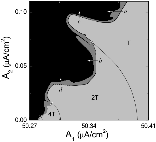
Figure 2: State diagram in the $A_{1}-A_{2}$ plane for $I_{dc}=100$ $\mu{\rm A/cm^{2}}$ and $f_{1}=26$ Hz in the quasiperiodically forced HH oscillator. Regular, SN, and chaotic regions are shown in light gray, gray, and black, respectively. In the regular region, the torus, the doubled torus, and the quadrupled torus exist in the regions denoted by $T$, $2T$, and $4T$, respectively, and the solid lines represent torus doubling bifurcation curves with terminal points denoted by crosses. SN attractors appear via fractalization, collision with a smooth unstable torus, and collision with a nonsmooth ring-shaped unstable set when passing the heavy solid line, the dashed line, and the dotted line, respectively.

From now on, we investigate the effect of quasiperiodic forcing on the period-doubling route to chaotic oscillation by changing $A_{1}$ and $A_{2}$ for $f_{1}=26$ Hz. Figure 2 shows a state diagram in the $A_{1}-A_{2}$ plane. Each state is characterized by the largest (nontrivial) Lyapunov exponent $\sigma_{1}$, associated with dynamics of the variable $\bf{x}$ [besides the (trivial) zero exponent, related to the phase variable $\theta$ of the quasiperiodic forcing] and the phase sensitivity exponent $\delta$. The exponent $\delta$ measures the sensitivity of the variable ${\bf x}$ with respect to the phase $\theta$ of the quasiperiodic forcing and characterizes the strangeness of an attractor PD . Regular quasiperiodic oscillations occur on smooth tori. A smooth torus that has a negative largest Lyapunov exponent (i.e., $\sigma_{1}<0$) and has no phase sensitivity (i.e., $\delta=0$) exists in the region denoted by $T$ and shown in light gray. When crossing a solid line, the smooth torus becomes unstable and bifurcates to a smooth doubled torus in the region represented by $2T$. Smooth quadrupled tori, bifurcated from doubled tori, also exist in the region denoted by $4T$. On the other hand, chaotic oscillating states with positive largest Lyapunov exponents ($\sigma_{1}>0$) exist in the region shown in black. Between these regular and chaotic regions, SN oscillating states that have negative largest Lyapunov exponents ($\sigma_{1}<0$) and positive phase sensitivity exponents $(\delta>0)$ exist in the region shown in gray. Due to their high phase sensitivity, SN oscillating states have a strange fractal phase space structure. Various dynamical routes to SN oscillations via gradual fractalization, collision with a smooth unstable torus, and collision with a nonsmooth ring-shaped unstable set will be discussed below.

When passing a heavy solid boundary curve in Fig. 2, a transition from a smooth torus to an SN attractor occurs via gradual fractalization NK . As an example, we study such transition to SN oscillations along the route $a$ by decreasing $A_{1}$ for $A_{2}=0.1$ $\mu{\rm A/cm^{2}}$. Figures 3(a)-3(c) show the time series of $V(t)$ for the quasiperiodic oscillation, the SN oscillation, and the chaotic oscillation when $A_{1}=50.41$, $50.374$, and $50.36$ $\mu{\rm A/cm^{2}}$, respectively. These regular, SN, and chaotic states are analyzed in terms of the largest Lyapunov exponent $\sigma_{1}$ and the phase sensitivity exponent $\delta$ in the Poincaré map. Projections of their corresponding attractors onto the $\theta-V$ plane are shown in Figs. 3(d)-3(f). For the regular state, a smooth torus exists in the $\theta-V$ plane [see Fig. 3(d)]. As $A_{1}$ is decreased, the smooth torus becomes more and more wrinkled and transforms to an SN attractor without apparent mediation of any nearby unstable invariant set SNA ; PNR . As an example, see an SN attractor in Fig. 3(e). This kind of gradual fractalization is the most common route to SN attractors. With further decrease in $A_{1}$, such an SN attractor turns into a chaotic attractor, as shown in Fig. 3(f).

A dynamical property of each attractor is characterized in terms of the largest Lyapunov exponent $\sigma_{1}$ (measuring the degree of sensitivity to initial conditions). The Lyapunov-exponent diagram (i.e., plot of $\sigma_{1}$ vs. $A_{1}$) is given in Fig. 3(g). When passing a threshold value of $A_{1}\simeq 50.377$ $\mu{\rm A/cm^{2}}$, an SN attractor appears. The graph of $\sigma_{1}$ for the SN attractor is shown in black, and its value is negative as in the case of smooth torus. However, as $A_{1}$ passes the chaotic transition point of $A_{1}\simeq 50.368$ $\mu{\rm A/cm^{2}}$, a chaotic attractor with a positive $\sigma_{1}$ appears. Although SN and chaotic attractors are dynamically different, both of them have strange geometry. To characterize the strangeness of an attractor, we investigate the sensitivity of the attractor with respect to the phase $\theta$ of the external quasiperiodic forcing PD . This phase sensitivity may be characterized by differentiating $\bf x$ with respect to $\theta$ at a discrete time $t=n$. Using Eq. (3), we may obtain the following governing equation for $\frac{\partial x_{i}}{\partial\theta}$ $(i=1,2,3,4)$,

$${\frac{d}{dt}}\left({\frac{\partial x_{i}}{\partial\theta}}\right)=\sum_{j=1}^{4}{\frac{\partial F_{i}}{\partial x_{j}}}\cdot{\frac{\partial x_{j}}{\partial\theta}}+{\frac{\partial F_{i}}{\partial\theta}},$$ (4)

where $(x_{1},x_{2},x_{3},x_{4})=(V,m,h,n)$ and $F_{i}$’s $(i=1,2,3,4)$ are given in Eq. (3). Starting from an initial point $({\bf{x}}(0),\theta(0))$ and an initial value $\partial\bf{x}/\partial\theta={\bf 0}$ for $t=0$, we may obtain the derivative values of $S^{(i)}_{n}$ $(\equiv\partial x_{i}/\partial\theta)$ at all subsequent discrete time $t=n$ by integrating Eqs. (3) and (4). One can easily see the boundedness of $S_{n}^{(i)}$ by looking only at the maximum

$$\gamma_{N}^{(i)}({\bf{x}}(0),\theta(0))=\max_{0\leq n\leq N}|S_{n}^{(i)}({\bf{x}}(0),\theta(0))|\,\,\,(i=1,2,3,4).$$ (5)

We note that $\gamma_{N}^{(i)}({{\bf x}(0)},\theta(0))$ depends on a particular trajectory. To obtain a “representative” quantity that is independent of a particular trajectory, we consider an ensemble of randomly chosen initial points $\{{\bf x}(0),\theta(0)\}$, and take the minimum value of $\gamma_{N}^{(i)}$ with respect to the initial orbit points PD ,

$$\Gamma_{N}^{(i)}=\min_{\{{\bf x}(0),\theta(0)\}}\gamma_{N}^{(i)}({\bf x}(0))\,\,\,(i=1,2,3,4).$$ (6)

Figure 3(h) shows a phase sensitivity function $\Gamma_{N}^{(1)}$, which is obtained in an ensemble containing 20 random initial orbit points $\{(V_{i}(0),m_{i}(0),h_{i}(0),n_{i}(0),\theta_{i}(0));i=1,\dots,20\}$ which are chosen with uniform probability in the range of $V_{i}(0)\in(-60,0)$, $m_{i}(0)\in(0.1,0.9)$, $h_{i}(0)\in(0.1,0.2)$, $n_{i}(0)\in(0.5,0.7)$ and $\theta_{i}(0)\in[0,1)$. For the case of the smooth torus in Fig. 3(d), $\Gamma_{N}^{(1)}$ grows up to the largest possible value of the derivative $|\partial x_{1}/\partial\theta|$ along a trajectory and remains for all subsequent time. Thus, $\Gamma_{N}^{(1)}$ saturates for large $N$ and hence the smooth torus has no phase sensitivity (i.e., it has smooth geometry). On the other hand, for the case of the SN attractor in Fig. 3(e), $\Gamma_{N}^{(i)}$ grows unboundedly with the same power $\delta$, independently of $i$,

$$\Gamma^{(i)}_{N}\sim N^{\delta}.$$ (7)

Here, the value of $\delta\simeq 2.39$ is a quantitative characteristic of the phase sensitivity of the SN attractor, and $\delta$ is called the phase sensitivity exponent. For obtaining satisfactory statistics, we consider 20 ensembles for each $A_{1}$, each of which contains 20 randomly chosen initial points and choose the average value of the 20 phase sensitivity exponents obtained in the 20 ensembles. Figure 3(i) shows a plot of $\delta$ versus $\Delta A_{1}$ $(=A_{1}-A_{1}^{*})$. Note that the value of $\delta$ monotonically increases from zero as $A_{1}$ is decreased away from the SN transition point $A_{1}^{*}$ $(\simeq 50.377$ $\mu{\rm A/cm^{2}})$. As a result of this phase sensitivity, the SN oscillating state has strange fractal geometry leading to aperiodic complex spikings, as in the case of chaotic oscillations [e.g., see Figs. 3(b) and 3(c)].

As a dashed boundary curve in Fig. 2 is crossed, another route to SN attractors appears through collision between a stable smooth doubled torus and its unstable smooth parent torus HH . As an example, we study this transition to SN oscillations along the route $b$ by decreasing $A_{1}$ for $A_{2}=0.06$ $\mu{\rm A/cm^{2}}$. Figure 4 shows a stable two-band torus (denoted by a solid curve) and an unstable smooth one-band parent torus (denoted by a short-dashed curve) for $A_{1}=50.348$ $\mu{\rm A/cm^{2}}$. The unstable parent torus is located in the middle of the two bands of the the stable torus. As $A_{1}$ is decreased, the bands of the stable torus becomes more and more wrinkled, while the unstable torus remains smooth [see Fig. 4(b)]. When $A_{1}$ passes a threshold value of $A_{1}\simeq 50.3469$ $\mu{\rm A/cm^{2}}$, the two bands of the stable torus touch its unstable parent torus at a dense set of $\theta$ values (not at all $\theta$ values). As a result of this phase-dependent (nonsmooth) collision between the stable doubled torus and its unstable parent torus, an SN attractor is born, as shown in Fig. 4(c). This SN attractor, containing the former bands of the torus as well as the unstable parent torus, has a positive phase sensitivity exponent (${\it i.e.,}$ $\delta>0$), inducing the strangeness of the SN attractor. However, its dynamics is nonchaotic because the largest Lyapunov exponent is negative (${\it i.e.,}$ $\sigma_{1}<0$). As another threshold value of $A_{1}\simeq 50.344$ $\mu{\rm A/cm^{2}}$ is passed, the SN attractor transforms to a chaotic attractor with a positive largest Lyapunov exponent $\sigma_{1}$ [see Fig. 4(d)].

A main interesting feature of the state diagram in Fig. 2 is the existence of “tongues” of quasiperiodic motion that penetrate into the chaotic region. The first-order (second-order) tongue lies near the terminal point (denoted by a cross) of the first-order (second-order) torus-doubling bifurcation curve. When crossing the upper boundary of the tongue (denoted by a dotted line), an intermittent SN attractor appears via phase-dependent collision of a stable torus with a nonsmooth ring-shaped unstable set Kim ; Kim2 . We first study the transition to an intermittent SN attractor along the route $c$ in the first-order tongue by increasing $A_{2}$ for $A_{1}=50.34$ $\mu{\rm A/cm^{2}}$. Figure 5(a) shows a smooth torus for $A_{2}=0.093$ $\mu{\rm A/cm^{2}}$. When passing a threshold value of $A_{2}\simeq 0.093\,35$ $\mu{\rm A/cm^{2}}$, a sudden transition to an intermittent SN attractor occurs, as shown in Fig. 5(b) for $A_{2}=0.093\,53$. Due to high phase sensitivity, this SN attractor with $\delta\simeq 3.15$ has a strange fractal structure, while its dynamics is nonchaotic because of a negative largest Lyapunov exponent ($\sigma_{1}\simeq-0.015$). A typical trajectory on the intermittent SN attractor spends a long stretch of time in the vicinity of the former torus, then it bursts out from this region and traces out a much larger fraction of the state space, and so on. To characterize the intermittent bursting, we use a small quantity $d^{*}$ for the threshold value of the magnitude of the deviation from the former torus. When the deviation is smaller (larger) than $d^{*}$, the intermittent attractor is in the laminar (bursting) phase. For each $A_{2}$, we follow a long trajectory until $10^{4}$ laminar phases are obtained in the Poincaré map $P$ and get the average of characteristic time $\tau$ between bursts. As shown in Fig. 5(c), the average value of $\tau$ exhibits a power-law scaling behavior,

$$\overline{\tau}\sim\Delta A_{2}^{-\gamma},~{}~{}\gamma\simeq 0.5,$$ (8)

where the overbar represents time averaging and $\Delta A_{2}^{*}=A_{2}-A_{2}^{*}$ $(A_{2}^{*}=0.093\,35)$. The scaling exponent $\gamma$ seems to be the same as that for the case of the quasiperiodically forced map PMR . As $A_{2}$ passes another threshold value of $A_{2}\simeq 0.0936$ $\mu{\rm A/cm^{2}}$, the SN attractor transforms to a chaotic attractor because the largest Lyapunov exponent $\sigma_{1}$ becomes positive, as shown in Fig. 5(d). Furthermore, using the rational approximation, the mechanism for the intermittent route to SN attractors will be investigated below. Thus, a smooth torus is found to transform to an intermittent SN attractor via phase-dependent collision with a nonsmooth ring-shaped unstable set.

We also study another intermittent route to SN attractors along the route $d$ in the second-order tongue by increasing $A_{2}$ for $A_{1}=50.3$ $\mu{\rm A/cm^{2}}$. Figure 5(e) shows a smooth two-band torus for $A_{2}=0.03$ $\mu{\rm A/cm^{2}}$. As $A_{2}$ passes a threshold value of $A_{2}\simeq 0.033\,45$ $\mu{\rm A/cm^{2}}$, a band-merging transition from a smooth doubled torus to a single-band SN attractor occurs Kim2 . Thus, an intermittent single-band SN attractor appears [e.g., see the intermittent SN attractor with $\sigma_{1}\simeq-0.029$ and $\delta\simeq 2.17$ in Fig. 5(f) for $A_{2}=0.0336$]. A typical trajectory of the second iterate of the Poincaré map $P$ (i.e. $P^{2}$) spends a long stretch of time near one of the two former attractors (i.e., smooth tori), then it bursts out of this region and comes close to the same or other former torus where it remains again for some time interval, and so on. As in the above case of intermittent route to SN attractors, we also obtain the $10^{4}$ laminar phases from a long trajectory in $P^{2}$, and get the average of characteristic time $\tau$ between bursts. As shown in Fig. 5(g), the average characteristic time shows a power-law scaling behavior,

$$\overline{\tau}\sim\Delta A_{2}^{-\gamma},~{}~{}\gamma\simeq 0.5,$$ (9)

where $\Delta A_{2}=A_{2}-A_{2}^{*}$ $(A_{2}^{*}=0.033\,45)$. The scaling exponent $\gamma$ seems to be the same as that for the case of the intermittent route to SN attractors occurring near the first-order tongue. Since the dynamical mechanism for the appearance of intermittent SN attractors near the first-order and second-order tongues are the same (i.e., an intermittent SN attractor appears via a phase-dependent collision between a smooth torus and a nonsmooth ring-shaped unstable set), the intermittent SN attractors for both cases seem to exhibit the same scaling behaviors. As $A_{2}$ is further increased and passes another threshold value of $A_{2}\simeq 0.0352$ $\mu{\rm A/cm^{2}}$, the SN attractor turns into a chaotic attractor with a positive largest Lyapunov exponent $\sigma_{1}$, as shown in Fig. 5(h).

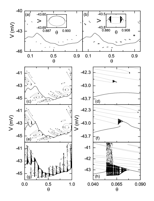
Figure 6: Intermittent transition to an SN attractor in the rational approximation. (a)-(b) Birth and evolution of a nonsmooth ring-shaped unstable set for $A_{2}=0.08$ $\mu{\rm A/cm^{2}}$ in the rational approximation of level $k=7$. (a) Smooth torus (denoted by a black curve) and ring-shaped unstable set for $A_{1}=50.3432$ $\mu{\rm A/cm^{2}}$. Each ring is composed of the attracting part (shown in black) and the unstable part (shown in gray). A magnified view of a ring is given in the inset. (b) Smooth torus (represented by a black curve) and an evolved ring-shaped unstable set for $A_{1}=50.343$ $\mu{\rm A/cm^{2}}$. As $A_{1}$ is decreased, the unstable part (shown in gray) in each ring becomes dominant. (c)-(h) Mechanism for the intermittent transition to an SN attractor along the route $c$ in Fig. 2 for $A_{1}=50.34$ $\mu{\rm A/cm^{2}}$. (c) Smooth torus and a ring-shaped unstable set for $A_{2}=0.089$ $\mu{\rm A/cm^{2}}$ [a magnified view near $\theta=0.065$ is given in (d)]. New rings appear inside or outside the old rings. (e) Nonsmooth attractor born via a phase-dependent (nonsmooth) collision between the smooth torus and a ring-shaped unstable set for $A_{2}=0.0904$ $\mu{\rm A/cm^{2}}$ [(f) is a magnified view near $\theta=0.065$]. (g) Intermittent SN attractor with $F_{7}$ gaps (born via an interior crisis) for $A_{2}=0.0915$ $\mu{\rm A/cm^{2}}$. (h) A magnified gap near $\theta=0.065$.

The dynamical mechanisms for the appearance of intermittent SN attractors near the tongues are the same, irrespectively of the tongue order. Here, we consider the case of the main first-order tongue, and using the rational approximation to the quasiperiodic forcing, we search for an unstable orbit that causes the intermittent transition via collision with the smooth torus for $A_{2}=0.08$ $\mu{\rm A/cm^{2}}$. For the inverse golden mean $\omega[=(\sqrt{5}-1)/2]$, its rational approximants are given by the ratios of the Fibonacci numbers, $\omega_{k}=F_{k-1}/F_{k}$, where the sequence of $\{F_{k}\}$ satisfies $F_{k+1}=F_{k}+F_{k-1}$ with $F_{0}=0$ and $F_{1}=1$. Instead of the quasiperiodically forced system with $\omega$, periodically forced systems with $\omega_{k}$ are studied in the rational approximation. As an example, we consider the rational approximation of level $k=7$. The rational approximation to the smooth torus (denoted by a black curve), composed of stable orbits with period $F_{7}(=13)$, is shown in Fig. 6(a) for $A_{1}=50.3432$ $\mu{\rm A/cm^{2}}$. We note that a ring-shaped unstable set, composed of $F_{7}$ small rings, lies near the smooth torus. At first, each ring is composed of the stable (shown in black) and unstable (shown in gray) orbits with period $F_{7}$ [see the inset in Fig. 6(a)]. However, as $A_{1}$ is changed such rings make evolution, as shown in Fig. 6(b) for $A_{1}=50.343$ $\mu{\rm A/cm^{2}}$. For fixed values of $A_{1}$ and $A_{2}$, the phase $\theta$ may be regarded as a “bifurcation parameter.” As $\theta$ is varied, a chaotic attractor appears via an infinite sequence of period-doubling bifurcations of stable periodic orbits in each ring, and then it disappears via a boundary crisis when it collides with the unstable $F_{7}$-periodic orbit [see the inset in Fig. 6(b)]. Thus, the attracting part (shown in black) of each ring is composed of the union of the originally stable $F_{7}$-periodic attractor, the higher $2^{n}F_{7}$-periodic $(n=1,2,\dots)$ and chaotic attractors born through the period-doubling cascade. On the other hand, the unstable part (shown in gray) of each ring consists of the union of the originally unstable $F_{7}$-periodic orbit [i.e., the lower gray line in the inset in Fig. 6(b)] and the destabilized $F_{7}$-periodic orbit [i.e., the upper gray line in the inset in Fig. 6(b)] via a period-doubling bifurcation. As the parameters, $A_{1}$ and $A_{2}$, are further changed, both the size and shape of the rings change, and eventually each ring is composed of a large unstable part (shown in gray) and a small attracting part (shown in black), as shown in Fig. 6(c) for $A_{1}=50.34$ $\mu{\rm A/cm^{2}}$ and $A_{2}=0.089$ $\mu{\rm A/cm^{2}}$ [a magnified view is given in Fig. 6(d)]. We also note that new rings appear inside or outside the “old” rings.

Finally, in terms of the rational approximation of level 7, we explain the mechanism for the intermittent transition occurring in the first-order tongue for $A_{1}=50.34$ $\mu{\rm A/cm^{2}}$ [see Figs. 5(a)-5(b)]. As we approach the border of the intermittent transition in the state diagram, the ring-shaped unstable set comes closer to the smooth torus, as shown in Fig. 6(c) for $A_{2}=0.089$ $\mu{\rm A/cm^{2}}$ [see a magnified view in Fig. 6(d)]. As $A_{2}$ passes a threshold value of $A_{2}\simeq 0.090\,305$ $\mu{\rm A/cm^{2}}$, a phase-dependent (nonsmooth) collision occurs between the smooth torus and the unstable part (shown in gray) of the nonsmooth ring-shaped unstable set. Then, the new attractor of the system contains the attracting part (shown in black) of the ring-shaped unstable set and becomes nonsmooth, which is shown in Fig. 6(e) for $A_{2}=0.0904$ $\mu{\rm A/cm^{2}}$ [see a magnified view in Fig. 6(f)]. As $A_{2}$ is further increased, the chaotic component in the rational approximation to the attractor increases, and eventually for $A_{2}\simeq 0.091\,202$ $\mu{\rm A/cm^{2}}$, it becomes suddenly widened via an interior crisis when it collides with the nearest ring [e.g., see Fig. 6(g)]. Then, $F_{7}(=13)$ “gaps,” where no attractors with period $F_{7}$ exist, are formed. A magnified gap is shown in Fig. 6(h). We note that this gap is filled by intermittent chaotic attractors. Thus, the rational approximation to the whole attractor consists of the union of the periodic and chaotic components. For this case, the periodic component is dominant, and hence the average largest Lyapunov exponent $(\langle\sigma_{1}\rangle\simeq-0.037)$ becomes negative, where $\langle\cdots\rangle$ denotes the average over the whole $\theta$. Hence, the rational approximation to the attractor becomes nonchaotic. We note that the 7th rational approximation to the attractor in Fig. 6(g) resembles the (original) intermittent SN attractor in Fig. 5(b), although the level of the rational approximation is low. In this way, the intermittent transition to an SN attractor occurs through two steps in the rational approximation: the phase-dependent (nonsmooth) collision and the interior crisis.

III Summary

We have numerically studied dynamical responses of the quasiperiodically forced HH neural oscillator and compared them with those for the periodically forced case. For the case of periodic forcing, a transition from a periodic to a chaotic oscillation has been found to occur via period doublings in both numerical and experimental works. Effect of the quasiperiodic forcing on this period-doubling route to chaotic oscillation has been investigated. In contrast to the case of periodic forcing, new type of SN oscillating states have been found to exist between the regular and chaotic oscillating states as intermediate ones. Due to their strange geometry, these SN oscillations lead to the occurrence of aperiodic complex spikings, as in the case of chaotic oscillations. Hence, SN oscillating states might be a dynamical origin for the complex spikings which are usually observed in cortical neurons. Various routes to SN oscillations via fractalization, collision with a smooth unstable torus, and collision with a nonsmooth ring-shaped unstable set have been identified, as in the quasiperiodically forced logistic map SNA . These SN responses are also found to occur in other neurons exhibiting period-doubling route to chaos (e.g., the Morris-Lecar neuron and the FitzHugh-Nagumo neuron) under quasiperiodic stimulus Kim5 . Finally, we suggest an experiment on the quasiperiodically forced squid giant axon and expect that SN spikings to be observed. However, the real biological environment is a noisy one. Hence, it is necessary to further investigate the effect of noise on the SN response for real experiment. This type of investigation is beyond the scope of the the present paper, and hence it is left as a future work.

Figure 1: Period-doubling route to chaos in the periodically forced HH oscillator for $I_{dc}=100$ $\mu{\rm A/cm^{2}}$ and $f_{1}=26$ Hz ($A_{2}=0$). Time series of $V(t)$ for (a) $A_{1}=50.42$ $\mu{\rm A/cm^{2}}$, (b) $A_{1}=50.33$ $\mu{\rm A/cm^{2}}$, and (c) $A_{1}=50.24$ $\mu{\rm A/cm^{2}}$, which correspond to the period-1, period-2, and chaotic states in the Poincaré map $P$ (solid circles represent stroboscopically sampled points in $P$), respectively. The largest Lyapunov exponent for the chaotic oscillation in (c) is $\sigma_{1}\simeq 0.096$. (d) Bifurcation diagram (i.e., plot of $V$ versus $A_{1}$) in $P$.

Figure 3: Appearance of an SN attractor via fractalization along the route $a$ in Fig. 2 for $A_{2}=0.1$ $\mu{\rm A/cm^{2}}$. Time series of $V(t)$ for (a) the quasiperiodic spiking state ($A_{1}=50.41$ $\mu{\rm A/cm^{2}}$), (b) the SN spiking state ($A_{1}=50.374$ $\mu{\rm A/cm^{2}}$), and (c) the chaotic spiking state ($A_{1}=50.36$ $\mu{\rm A/cm^{2}}$). Projections of attractors onto the $\theta-V$ plane in the Poincaré map are shown for (d) the smooth torus [corresponding to (a)], (e) the SN attractor [corresponding to (b)], and (f) the chaotic attractor [corresponding to (c)]. (g) Lyapunov-exponent diagram (i.e., plot of $\sigma_{1}$ vs. $A_{1}$); $\sigma_{1}$ for the SN attractor is shown in black. (h) Phase sensitivity functions $\Gamma_{N}^{(1)}$ are shown for the smooth torus ($T$) [(d)] and the SN attractor (SNA) [(e)]. For the case of the SN attractor, the graph is well fitted with a dashed straight line with slope $\delta\simeq 2.39$. (i) Plot of the phase sensitivity exponent $\delta$ versus $\Delta A_{1}$ $(=A_{1}-A_{1}^{*})$ for the SN attractor; $A_{1}^{*}\simeq 50.377$.

Figure 4: Appearance of an SN attractor via phase-dependent (nonsmooth) collision between a stable two-band torus and its unstable smooth parent torus along the route $b$ in Fig. 2 for $A_{2}=0.06$ $\mu{\rm A/cm^{2}}$. Stable two-band torus (denoted by a solid curve) and its unstable smooth torus (represented by a short-dashed curve) for (a) $A_{1}=50.348$ $\mu{\rm A/cm^{2}}$ and (b) $A_{1}=50.347$ $\mu{\rm A/cm^{2}}$. (c) SN attractor with $\sigma_{1}\simeq-0.015$ and $\delta\simeq 3.77$ for $A_{1}=50.346$ $\mu{\rm A/cm^{2}}$. (d) Chaotic attractor with $\sigma_{1}\simeq 0.038$ for $A_{1}=50.34$ $\mu{\rm A/cm^{2}}$.

Figure 5: Appearance of intermittent SN attractors. (a)-(d) Appearance of an intermittent SN attractor along the route $c$ in Fig. 2 for $A_{1}=50.34$ $\mu{\rm A/cm^{2}}$. (a) Smooth torus with $\sigma_{1}\simeq-0.071$ for $A_{2}=0.093$ $\mu{\rm A/cm^{2}}$. (b) Intermittent SN attractor with $\sigma_{1}\simeq=-0.015$ and $\delta\simeq 3.15$ for $A_{2}=0.09353$ $\mu{\rm A/cm^{2}}$. (c) Plot of ${\rm log_{10}}\overline{\tau}$ vs. ${\rm log_{10}}\Delta A_{2}$. The graph is well fitted with a dashed straight line with slope $\gamma\simeq 0.5$. Here $\overline{\tau}$ is the average characteristic time between bursts and $\Delta A_{2}=A_{2}-A_{2}^{*}$ $(A_{2}^{*}=0.093\,35$ $\mu{\rm A/cm^{2}})$. For each $\Delta A_{2}$, $\overline{\tau}$ is calculated from $10^{4}$ laminar phases in the Poincaré map $P$. (d) Chaotic attractor with $\sigma_{1}\simeq 0.083$ for $A_{2}=0.095$ $\mu{\rm A/cm^{2}}$. (e)-(h) Band-merging transition from a two-band torus to an intermittent single-band SN attractor along the route $d$ in Fig. 2 for $A_{1}=50.3$ $\mu{\rm A/cm^{2}}$. (e) Smooth two-band torus with $\sigma_{1}\simeq-0.135$ for $A_{2}=0.03$ $\mu{\rm A/cm^{2}}$. (f) Intermittent single-band SN attractor with $\sigma_{1}\simeq-0.029$ and $\delta\simeq 2.17$ for $A_{2}=0.0336$ $\mu{\rm A/cm^{2}}$. (g) Plot of ${\rm log_{10}}\overline{\tau}$ vs. ${\rm log_{10}}\Delta A_{2}$. The graph is well fitted with a dashed straight line with slope $\gamma\simeq 0.5$. Here $\overline{\tau}$ is the average characteristic time between bursts and $\Delta A_{2}=A_{2}-A_{2}^{*}$ $(A_{2}^{*}=0.033\,45$ $\mu{\rm A/cm^{2}}$). For each $\Delta A_{2}$, $\overline{\tau}$ is calculated from $10^{4}$ laminar phases in $P^{2}$. (h) Chaotic attractor with $\sigma_{1}\simeq 0.079$ for $A_{2}=0.04$ $\mu{\rm A/cm^{2}}$.

- (1) M. R. Guevara, L. Glass, and A. Shrier, Science 214, 1350 (1981); L. Glass, M. R. Guevara, A. Shrier, and R. Perez, Physica D 7, 89 (1983).
- (2) K. Aihara, T. Numajiri, G. Matsumoto, and M. Kotani, Phys. Lett. A 116, 313 (1986); N. Takahashi, Y. Hanyu, T. Musha, R. Kubo, and G. Matsumoto, Physica D 43, 318 (1990); D. T. Kaplan, J. R. Clay, T. Manning, L. Glass, M. R. Guevara, and A. Shrier, Phys. Rev. Lett. 76, 4074 (1996).
- (3) K. Aihara, Scholarpedia 3(5): 1786 (2008); see also references therein.
- (4) L. Glass and M. C. Mackey, From Clocks to Chaos (Princeton University Press, Princeton, 1988).
- (5) R. Stoop, K. Schindler, and L.A. Bunimovich, Neurosci. Res. 36, 81 (2000); Nonlinearity 13, 1515 (2000).
- (6) M. Ding and J. A. S. Kelso, Int. J. Bifurcation Chaos Appl. Sci. Eng. 2, 295 (1992).
- (7) U. Feudel, S. Kuznetsov, and A. Pikovsky, Strange Nonchaotic Attractors (World Scientific, Singapore, 2006).
- (8) A. Prasad, S. S. Negi, and R. Ramaswamy, Int. J. Bifuraction Chaos Appl. Sci. Eng. 11, 291 (2001); U. Feudel, C. Grebogi, and E. Ott, Phys. Rep. 290, 11 (1997).
- (9) C. Grebogi, E. Ott, S. Pelikan, and J. A. Yorke, Physica D 13, 261 (1984).
- (10) K. Kaneko, Prog. Theor. Phys. 72, 202 (1984); T. Nishikawa and K. Kaneko, Phys. Rev. E 54, 6114 (1996).
- (11) J. F. Heagy and S. M. Hammel, Physica D 70, 140 (1994).
- (12) A. S. Pikovsky and U. Feudel, Chaos 5, 253 (1995).
- (13) A. Prasad, V. Mehra, and R. Ramaswamy, Phys. Rev. Lett. 79, 4127 (1997).
- (14) S.-Y. Kim, W. Lim, and E. Ott, Phys. Rev. E 67, 056203 (2003); S.-Y. Kim and W. Lim, J. Phys. A 37, 6477 (2004).
- (15) W. Lim and S.-Y. Kim, Phys. Lett. A 335, 383 (2005).
- (16) W. Lim and S.-Y. Kim, Phys. Lett. A 355, 331 (2006); S.-Y. Kim and W. Lim, ibid. 334, 160 (2005).
- (17) J.-W. Kim, S.-Y. Kim, B. Hunt, and E. Ott, Phys. Rev. E 67, 036211 (2003).
- (18) W. L. Ditto, M. L. Spano, H. T. Savage, S. N. Rauseo, J. Heagy, and E. Ott, Phys. Rev. Lett. 65, 533 (1990); W. X. Ding, H. Deutsch, A. Dinklage, and C. Wilke, Phys. Rev. E 55, 3769 (1997); B. P. Bezruchko, A. P. Kuznetsov, and Y. P. Seleznev, Phys. Rev. E 62, 7828 (2000); K. Thamilmaran, D. V. Senthikumar, A. Venkatesan, and M. Lakshmanan, Phys. Rev. E 74, 036205 (2006).
- (19) A. L. Hodgkin and A. F. Huxley, J. Physiol. (London) 117, 500 (1952).
- (20) K. Aihara, G. Matsumoto, and Y. Ikegaya, J. Theor. Biol. 109, 249 (1984).
- (21) D. Hansel, G. Mato, and C. Meunier, Europhys. Lett. 23, 367 (1993).
- (22) A. J. Lichtenberg and M. A. Lieberman, Regular and Stochastic Motion (Springer-Verlag, New York, 1983), p. 283.
- (23) E. M. Izhikevich, Int. J. Bifurcation Chaos Appl. Sci. Eng. 10, 1171 (2000).
- (24) S.-G. Lee, A. Neiman, and S. Kim, Phys. Rev. E 57, 3292 (1998).
- (25) W. Lim, S.-Y. Kim, and Y. Kim (unpublished).