Optical antennas as nanoscale resonators

Mario Agio,^∗a

Recent progress in nanotechnology has enabled us to fabricate subwavelength architectures that function as antennas for improving the exchange of optical energy with nanoscale matter. We describe the main features of optical antennas for enhancing quantum emitters and review designs that increase the spontaneous emission rate by orders of magnitude from the ultraviolet up to the near-infrared spectral range. To further explore how optical antennas may lead to unprecedented regimes of light-matter interaction, we draw a relationship between metal nanoparticles, radio-wave antennas and optical resonators. Our analysis points out how optical antennas may function as nanoscale resonators and how these may offer unique opportunities with respect to state-of-the-art microcavities.

1 Introduction

The dramatic advances of nanotechnology experienced in recent years have fueled much interest in optical antennas as devices for managing the concentration, absorption and radiation of light at the nanometer scale.^{1, 2, 3, 4} In fact, the amount of activities on this topic has grown very rapidly in various fields of research, spanning physics, chemistry, electrical engineering, biology, and medicine to cite a few.^{5, 6, 7, 8, 9, 10, 11} At a more fundamental level, these systems may enhance the radiation properties of quantum emitters, such as atoms and molecules,¹² an endeavor that dates back to the onset of field-enhanced spectroscopy.^{13, 14, 15, 16}

Somewhat in parallel, the past decades have witnessed great progress in the fundamentals and applications of optical resonators.^{17, 18, 19} In particular, recent developments in photonic crystals have enabled the realization of miniaturized cavities with mode volumes of the order of one cubic wavelength and huge quality factors.^{20, 21} Obtaining resonators with even smaller dimensions is a current research challenge, which pushes optical physics and nanofabrication into new pathways.

A promising strategy relies on metal nanocavities, which use metal mirrors to confine light into tight volumes. They are being explored, for instance, to realize ultrasmall lasers,^{22, 23, 24} and to enhance the spontaneous emission (SE) rate of quantum emitters.^{25, 26, 27} As resonators are pushed towards deep subwavelength dimensions, it becomes apparent that their differences with respect to optical antennas begin to vanish. In fact, several phenomena and functionalities are investigated using antenna architectures treated as nanoscale cavities.^{28, 29, 30, 31, 32, 33}

To gain insight on this exciting scenario for light-matter interaction, we attempt to uncover the relationship between optical antennas and resonators. First, we review a number of empirical rules to engineer optical antennas that lead to a strong enhancement of the SE rate with minimal losses caused by absorption in real metals.³⁴ Moreover, we describe designs that are fully compatible with state-of-the-art nanofabrication and highlight effects related to the antenna composition and shape.^{34, 35, 36, 37, 38}

Next, we consider a simplified antenna model and discuss basic properties starting from analytical expressions. Since the physical dimensions are smaller than the operating wavelength, we base our analysis on the fundamental limitations of electrically small antennas.³⁹ We thus select a few popular resonator designs^{18, 21} and compare their figures of merit with those of optical antennas.³⁶ We show that the enhancement of light-matter interaction is comparable to that achievable with state-of-the-art cavities. Therefore, despite absorption by real metals, there is a window of opportunity where optical antennas may function as nanoscale resonators with a tiny device footprint and manageable losses.

There is another important advantage. Having a low quality factor, optical antennas are fully compatible with methods and techniques of ultrafast spectroscopy⁴⁰ and coherent control.⁴¹ We will return to these aspects in the conclusions.

2 Optical antennas

Optical antennas are metal nanostructures that convert strongly localized energy into radiation and vice versa with a high throughput.¹ They share several concepts of radio-wave antennas, but they also have distinctive features, which are illustrated in Fig. 1. First, the coupling between the antenna and its load is not via wired electric currents, but via displacement currents proportional to the near field, which makes the interaction strongly position and polarization dependent.⁴² Second, the load is typically a quantum system, like an atom or a molecule, and as such it is affected by quantum electrodynamics (QED) phenomena associated with the modification of the local electromagnetic environment.^{43, 44} Third, metals at optical frequencies are not perfect conductors and their optical properties are strongly affected by the existence of surface plasmon-polariton (SPP) resonances.^{42, 45} These modes are tightly confined and can be controlled at the nanoscale by shaping metals using state-of-the-art nanofabrication.⁴⁶ Furthermore, they also depend on intrinsic material properties such as the optical constants⁴⁷ and the electron mean free path.⁴⁸ Fourth, in optics we often work with focused beams and guided waves. These should be considered as relevant degrees of freedom for interfacing light with optical antennas.^{49, 50, 51, 52} In summary, optical antennas represent a truly interdisciplinary effort that involves electrical engineering, physical chemistry, quantum optics, materials science as well as optics and photonics. In this respect, there are ongoing efforts aimed at their understanding and modeling within the established and powerful formalism developed for radio-wave antennas. These include the definition of antenna resonance wavelength⁵³ and impedance.⁵⁴, ⁵⁵

In Sec. 2.1-2.3 we explain how optical antennas may enhance light-matter interaction at the level of a single quantum emitter and how this can be optimized by design. In Sec. 2.4 we analyze the main effects associated with the antenna composition and background medium. Moreover, in Sec. 3 we make use of radio-wave antenna theory to formulate a link with nanoscale resonators. We thus plan to cover most of the aspects illustrated in Fig. 1, hoping to show how an interdisciplinary approach may facilitate our understanding and also reveal the exciting opportunities of this vibrant research field.

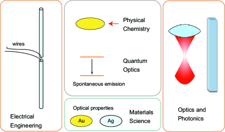
Fig.  1: Optical antennas: a truly interdisciplinary research field that involves diverse areas like electrical engineering, physical chemistry, quantum optics, materials science, as well as optics and photonics.

2.1 Enhancement and quenching of fluorescence

We review the basic phenomena that take place when a quantum emitter interacts with a metal nanostructure and try to make a connection with concepts familiar to radio-wave antennas. We limit our analysis to the weak excitation limit, where the semi-classical theory of light-matter interaction is greatly simplified.⁵⁶ The relevant quantities that need to be considered when an emitter is coupled to an optical antenna are the field enhancement, the SE rate, the quantum yield and the radiation pattern. The last topic does not fall in the focus of this work and will not be addressed.^{59, 60, 61, 57, 62, 58}

Under weak resonant excitation the fluorescence signal can be approximated by the formula

$$S_{o}=\xi_{o}\eta_{o}|\mathbf{E}_{o}\cdot\mathbf{d}|^{2}.$$ (1)

The parameter $\xi_{o}$ represents the collection efficiency, $\mathbf{d}$ is the transition electric dipole moment, and $\mathbf{E}_{o}$ is the electric field at the emitter position. $\eta_{o}=\Gamma_{\mathrm{r}}^{o}/\Gamma_{\mathrm{t}}^{o}$ is the quantum yield and it corresponds to the ratio between the radiative and total decay rates. The latter takes into account the fact that the excited state can also lose energy via non-radiative channels, i.e. $\Gamma_{\mathrm{t}}^{o}=\Gamma_{\mathrm{r}}^{o}+\Gamma_{\mathrm{nr}}^{o}$. The label $o$ indicates that these quantities refer to an isolated emitter.

2.1.1 Field enhancement.  

Away from saturation the excitation rate may be increased by placing the emitter near a nanostructure that modifies the electric field. Engineering textbooks do not discuss the intensity enhancement $K$, because it is not an important design parameter for radio-wave antennas,⁶³ while in optical domain the phenomenon has been thoroughly investigated in the context of surface-enhanced Raman spectroscopy.^{15, 16} Pioneering works based on polarizability models indicated the SPP resonance and the lighting rod effect as the two most important electromagnetic enhancement mechanisms.⁴² The latter can be intuitively explained by considering the increase in the surface charge density $\sigma$ with the curvature of a metal surface.⁶⁴ Since the near field is directly proportional to $\sigma$, nanoparticles with sharp tips tend to exhibit larger enhancements than nanospheres. Other strategies to improve the strength of the near field include the exploitation of nanoscale gaps between two nanoparticles,⁶⁵ the suppression of radiative broadening⁶⁶ and the choice of different metals.^{67, 68} These basic design concepts have been applied with more breadth and detail in the subsequent years, when computational methods for nano-optics have become available.⁶⁹

2.1.2 Decay rates.  

It is well known that the SE rate is not an intrinsic property of an atom or a molecule, but it also depends on the local electromagnetic environment.⁷⁰ Its modification can be obtained by computing the power emitted by a classical dipole placed in proximity of the optical antenna. The correspondence between quantum and classical theory is valid if the normalized quantities are used,^{14, 71, 72}

$$\frac{\Gamma_{\mathrm{r}}}{\Gamma_{\mathrm{r}}^{o}}=\frac{P_{\mathrm{r}}}{P_{o}},$$ (2)

where $P_{o}$ and $P_{\mathrm{r}}$ are the power radiated by a classical dipole in free space and near an optical antenna, respectively.

We take advantage of the reciprocity argument⁶³ to state that a strong $K$ is associated with a strong modification of the radiative decay rate. Indeed, it can be shown that for an antenna that does not modify the radiation pattern of the emitter these two quantities are exactly equal.⁷³ Therefore, one could simply refer to the design strategies discussed in the previous section to obtain a large modification of the SE rate.⁷⁴

Because part of the emitted power is absorbed by metal losses, a full characterization of the system requires the calculation of both radiative $\Gamma_{\mathrm{r}}$ and non-radiative $\Gamma_{\mathrm{nr}}$ decay rates.^{14, 75} The total decay rate $\Gamma_{\mathrm{t}}$ is thus $\Gamma_{\mathrm{r}}+\Gamma_{\mathrm{nr}}+\Gamma_{\mathrm{nr}}^{o}$. The corresponding classical quantities are easily derived from Poynting theorem,⁶⁴ which leads to

$$\frac{\Gamma_{\mathrm{r}}+\Gamma_{\mathrm{nr}}}{\Gamma_{\mathrm{r}}^{o}}=\frac{P_{\mathrm{t}}}{P_{o}},$$ (3)

where $P_{\mathrm{t}}$ is the total power dissipated by the dipole.

2.1.3 Antenna efficiency.  

The enhancement of $\Gamma_{\mathrm{nr}}$ requires some attention. We follow an approach borrowed from antenna theory,⁶³ where the antenna efficiency $\eta_{\mathrm{a}}$ is defined as the ratio between the radiated power and the total power transferred from the load to the antenna. For the case of a quantum load, i.e. an atom or a molecule, it reads $\eta_{\mathrm{a}}=\Gamma_{\mathrm{r}}/(\Gamma_{\mathrm{r}}+\Gamma_{\mathrm{nr}})$ and the modified quantum yield $\eta$ takes the expression⁷⁶

$$\eta=\dfrac{\eta_{o}}{(1-\eta_{o})\Gamma_{\mathrm{r}}^{o}/\Gamma_{\mathrm{r}}+\eta_{o}/\eta_{\mathrm{a}}}.$$ (4)

In comparison with the field enhancement, in the past years less attention has been dedicated to the improvement of $\eta_{\mathrm{a}}$. It turns out that the latter is mostly affected by higher-order SPP modes, which are strongly damped by absorption.⁴³, ⁷⁷, ⁴⁴ In fact, $\Gamma_{\mathrm{nr}}$ takes over $\Gamma_{\mathrm{r}}$ as the emitter approaches the metal surface, because the source field becomes so inhomogeneous across the antenna that multipoles are excited more efficiently. Moreover, there is a contrast between $K$ and $\eta_{\mathrm{a}}$. For example, while radiative effects reduce the near-field strength,⁶⁶ they tend to increase $\eta_{\mathrm{a}}$.⁷⁸

Obtaining a large increase of the SE rate without compromising $\eta_{\mathrm{a}}$ is thus a non trivial task. In what follows we show that this is not a fundamental limitation and discuss situations where the SE rate is enhanced by more than three orders of magnitude without quenching.

2.2 Design rules

The key design principles for achieving a strong modification of the SE rate with minimal suffering from $\Gamma_{\mathrm{nr}}$ can be summarized as follows. First, tailor the geometry such that the SPP resonance of the antenna lies in a spectral region that minimizes dissipation in the metal. Second, choose elongated objects to benefit from strong near fields at sharp corners. Third, adjust the emitter orientation such that its electric dipole moment is aligned with that of the antenna. Fourth, ensure that in the antenna higher order SPP modes are spectrally separated from the dipolar one.³⁴ Fifth, choose the antenna volume such that radiation is stronger than absorption.^{78, 79}

To exemplify these rules we consider the emission of a dipole close to an elliptical gold nanoparticle. Its SPP resonance is located in the near-infrared region, where the imaginary part of the dielectric function of gold is smaller.⁸⁰ Moreover, $K$ is expected to be stronger at the nanoparticle apex. As shown in Fig. 2a, we see that, although both $\Gamma_{\mathrm{􏰫r}}$ and $\Gamma_{\mathrm{nr}}$ experience a considerable enhancement, $\Gamma_{\mathrm{􏰫r}}$ is larger than $\Gamma_{\mathrm{nr}}$ at the SPP resonance of the long axis. Figure 2b plots the distance dependence of the decay rates at the long-axis SPP resonance, illustrating that $\Gamma_{\mathrm{􏰫r}}$ dominates for all separations larger than 3 nm. The strong quenching observed at shorter wavelengths is attributed to the excitation of higher-order multipoles, which are spectrally separated from the SPP dipole mode.³⁴

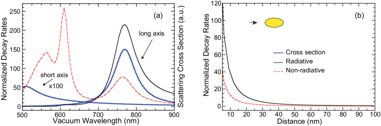
Fig.  2: Normalized decay rates for an emitter coupled to a gold ellipse (long axis = 60 nm, short axis = 10 nm, backround refractive index $n_{\mathrm{b}}$=1.7, two-dimensional model). (a) Wavelength dependence for a particle-emitter distance of 3 nm. The scattering cross section of the antenna is also plotted. (b) Distance dependence for the wavelength $\lambda$ = 770 nm. The emitter is oriented as shown in the inset. Figure adapted with permission from Ref. ³⁴. Copyright (2007) by the Optical Society of America.

2.3 Shape dependence

In Fig. 2 we have shown that changing the shape of the optical antenna can have a huge impact on its performances. In this section we analyze this in more detail, with emphasis on the modification of the SE rate and $\eta_{\mathrm{a}}$. In particular, we pay attention to systems and parameters that are within the reach of standard nanofabrication methods and of the common experimental techniques used in nano-optics.⁹

2.3.1 Adding a second nanoparticle.  

A better comparison with the single nanoparticle case can be seen if the molecule is at a fixed distance from one of the two nano-objects, while the other one is approached from far away.³⁵ The inset of Fig. 3 schematically shows how the coupling between emitter and antenna is modified by changing the distance $d$.

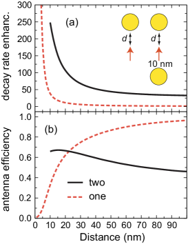
Fig.  3: Emitter coupled to one or two 100 nm gold nanospheres in air. Enhancement of the SE rate (a) and $\eta_{\mathrm{a}}$ (b) at $\lambda=580$ nm. The inset describes the coupling scheme. Figure adapted with permission from Ref. ³⁵. Copyright (2007) by SPIE.

The enhancement of the SE rate is plotted in Fig. 3a as a function of $d$. When both nanoparticles are close to the emitter, the increase is clearly larger than for a single one. Figure 3b shows that for one nanoparticle $\eta_{\mathrm{a}}$ rapidly drops to zero when the distance becomes smaller than 20 nm,^{81, 82, 83, 44} whereas for two nanoparticles it slightly increases and then decreases until quenching (not shown), but at shorter distances than for the previous case. Thus, the data from Fig. 3a and b highlight the competition between the SE rate enhancement and $\eta_{\mathrm{a}}$. Note that the balance between them is clearly different for one and two nanoparticles.

2.3.2 Changing the nanoparticle apex.  

To further discuss how the nanoparticle shape affects the antenna performances, we focus on the wavelength range between 600 nm and 1100 nm, which covers the emission spectrum of relevant nanoscale light emitters.^{84, 85, 86, 87} Because the enhancement is maximum when the emitter is placed at and oriented along the nanoparticle long axis, we only consider this situation. Furthermore, to treat a more experimentally feasible situation, we set the distance between emitter and nanoparticle to 10 nm.

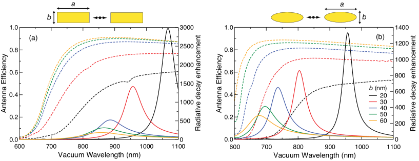
Fig.  4: Antenna efficiency (dashed curves) and radiative decay enhancement (solid curves) for an emitter coupled to two gold nanorods (a) and nanospheroids (b) in glass as a function of the aspect ratio for $a$=80 nm. Figure adapted with permission from Ref. ³⁶. Copyright (2008) by IOP Publishing.

We compare nanospheroids^{43, 88} with gold nanorods.^{3, 89} Figure 4a shows that the SPP resonance peak red shifts when the nanorod short axis $b$ decreases. Therefore, by tuning the aspect ratio $a/b$ one can easily place the SPP resonance at the desired spectral location.⁸⁹ The increase of the radiative decay rate is close to 3000 for wavelengths around 1100 nm. However, when the resonance moves towards the visible spectrum, the enhancement drops very rapidly. As shown in Fig. 4a, $\eta_{\mathrm{a}}$ increases with the nanorod volume, i.e. as $b$ becomes larger. Unfortunately, the largest improvement correspond to the lowest efficiency because a higher aspect ratio implies a reduced volume.⁷⁹

The steep decrease of the enhancement upon reduction of the aspect ratio stems from the fact that the nanorods ends are flat. In replacing nanorods with nanospheroids we identify three important aspects. First, for high aspect ratios the nanospheroids exhibit smaller enhancements. Second, for low aspect ratios the enhancement decreases more slowly and the SPP resonance is less red-shifted, as shown in Fig. 4b. Third, $\eta_{\mathrm{a}}$ reaches its plateau already at wavelengths close to 650 nm if the aspect ratio is less than 2. Compared to nanorods the enhancement is larger at shorter wavelengths because a smaller aspect ratio is partially compensated by a sharper nanoparticle apex. A more detailed comparison of the two antenna systems can be found in Ref. ³⁶. These results highlight the fact that experiments require great control over the nanoparticle shape, especially if large enhancements are desired.

2.3.3 The conical antenna.  

An important issue is that $\eta_{\mathrm{a}}$ and the enhancement of SE are maximal for different antenna parameters. Can we improve the antenna design to increase $\Gamma_{\mathrm{t}}$ without decreasing $\eta_{\mathrm{a}}$ and losing control on the spectral position of the resonance? A simple solution is to use a nanocone, where one end can be sharp to increase $K$ and the SE rate, whereas the other end can be larger for increasing the volume, hence $\eta_{\mathrm{a}}$.³⁸

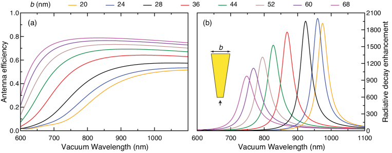
Fig.  5: (a) Antenna efficiency and (b) radiative decay enhancement as a function of the base diameter $b$. The nanocone is in air, it is 140 nm long and it has a tip diameter of 20 nm. Figure adapted with permission from Ref. ³⁸. Copyright (2010) by the American Chemical Society.

Figure 5 displays the radiative decay enhancement and $\eta_{\mathrm{a}}$ for single nanocones as a function of the base diameter $b$. The rate increases slightly and then decreases, confirming that there exists an optimal value for $b$.^{90, 91} On the other hand, $\eta_{\mathrm{a}}$ grows with $b$ because the antenna volume increases. An important advantage with respect to nanorods and nanospheroids is that here the resonance can be spectrally tuned by changing the nanocone angle, without a significant loss of enhancement. Note that the enhancement factor is as high as 2000 for a conical and 8000 for a bi-conical antenna (not shown).³⁸

2.4 Materials dependence

We have discussed examples where the antenna properties are tuned by changing its shape and size. While these degrees of freedom offer a wide range of performances, there are situations where other parameters may be adjusted. For instance, recent works have investigated the optical response of copper,⁹² aluminum^{93, 94, 95, 96, 37} and palladium⁹⁷ nanoparticles. While previous theoretical studies focused on $K$,^{67, 68} here we discuss the modification of the SE rate and $\eta_{\mathrm{a}}$. We choose nanospheroids as a model system and review designs that cover the spectral range from the ultraviolet to the near-infrared.^{37, 79}

2.4.1 Background medium.  

First, we wish to illustrate how the enhancement of the radiative decay rate and $\eta_{\mathrm{a}}$ depend on the background index. Figure 6a shows that for an emitter coupled to a gold nanospheroid even a small change in the refractive index shifts the SPP resonance by more than hundred nanometers. At the same time, the resonance gets wider because radiative broadening increases with the refractive index.⁶⁶ That also explains the small decrease in the enhancement. Note that the shift of the SPP resonance towards shorter wavelengths improves $\eta_{\mathrm{a}}$. For instance, it is larger than 70% around 650 nm if the antenna is in air.

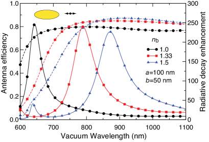
Fig.  6: Radiative decay enhancement (solid curves) and antenna efficiency (dashed curves) for an emitter coupled to a gold nanospheroid. Dependence on the background index $n_{\mathrm{b}}$. Figure adapted with permission from Ref. ³⁷. Copyright (2009) by the American Scientific Publishers.

2.4.2 Gold and copper.  

The real part of the dielectric function of the two materials is quite similar, whereas the imaginary part is larger for copper.^{47, 80} Figure 7 shows the radiative decay enhancement and $\eta_{\mathrm{a}}$ for an emitter coupled to a copper nanospheroid. Compared to gold antennas the enhancement is smaller and the resonances are broader, as expected from the larger imaginary part. Moreover, $\eta_{\mathrm{a}}$ is lower, but it shows the same trend as gold antennas.

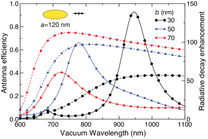
Fig.  7: Radiative decay enhancement (solid curves) and antenna efficiency (dashed curves) for an emitter coupled to a copper nanospheroid in glass. Figure adapted with permission from Ref. ³⁷. Copyright (2009) by the American Scientific Publishers.

2.4.3 Silver and aluminum.  

Silver has a higher plasma frequency than gold so that the antenna resonance is shifted towards shorter wavelengths. On the other hand the imaginary part of the dielectric function drops to lower values, with immediate benefits for $\eta_{\mathrm{a}}$.⁴⁷

Aluminum has an even higher plasma frequency than silver.⁹⁸ Even if the imaginary part is significantly larger than in the noble metals, in the region below 600 nm the large and negative real part ensures that the skin depth is sufficiently small to prevent significant absorption losses.

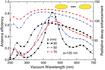
Fig.  8: Radiative decay enhancement (solid curves) and antenna efficiency (dashed curves) for an emitter coupled to two aluminum nanospheroids in air. Figure adapted with permission from Ref. ³⁷. Copyright (2009) by the American Scientific Publishers.

The antenna efficiency and the radiative decay enhancement for an emitter coupled to two aluminum nanospheroids is provided in Fig. 8. The performances are not as high as for the same geometry made from other materials.³⁷ Since $\eta_{\mathrm{a}}$ is large the reason for that should be attributed to radiative broadening rather than to losses.⁶⁶ Indeed, optimizations of $K$ have shown that the SPP resonance should be tuned around 200-300 nm.⁶⁸ Aluminum is thus more suitable for applications in the ultraviolet spectral region.^{99, 95}

3 Towards nanoscale cavities

We have shown how optical antennas may increase the SE rate by orders of magnitude with minimal suffering from absorption losses. These settings are very promising for implementing the functionalities of microresonators at the nanoscale. It is therefore instructive to translate the antenna performances into the common parameters of an optical cavity, i.e. quality factor, mode volume, Purcell factor and device footprint.

Recent works have discussed the enhancement of light-matter interaction by optical antennas and metal nanocavities using the mode-volume picture and the Purcell factor.^{103, 100, 101, 102} Here we combine field-enhanced spectroscopy, antenna theory and cavity QED to express figures of merit and scaling laws that may provide useful insight on the opportunities offered by optical antennas seen as nanoscale resonators. Furthermore, we pay attention to the antenna efficiency and study how it constrains the other performances.

3.1 From antenna theory to nanoscale resonators

First, we briefly review the formulation of cavity QED in the perturbative regime, which is the same level of theory used in the previous sections for optical antennas. For convenience we set $\Gamma_{\mathrm{nr}}^{o}=0$, and write $\Gamma_{\mathrm{r}}^{o}=\Gamma_{o}$ and $\Gamma_{\mathrm{t}}=\Gamma$. Next, we discuss the relationship between the Purcell factor and the modification of the SE rate by optical antennas, with emphasis on the local density of photonic states. We then establish a connection between $K$ and the near-field zone of a radio-wave antenna.

3.1.1 Cavity quantum electrodynamics.  

In free space the quantized electromagnetic field is expressed by

$$\mathbf{E}(\mathbf{r})=i\sum_{\mu}\sqrt{\dfrac{\hbar\omega_{\mu}}{2\epsilon_{0}V}}\mathbf{e}_{\mu}\left(\hat{a}_{\mu}e^{i\mathbf{k\cdot r}}-\mathrm{h.c.}\right),$$ (5)

where h.c. means Hermitian conjugation of the preceding term. $V$ is the quantization volume, $\mathbf{e}_{\mu}$ is the polarization versor and $\hat{a}_{\mu}$ is the destruction operator for one photon in the mode $\mu$ of energy $\hbar\omega_{\mu}$.⁵⁶ Using Eq. (5) in Fermi golden rule we obtain

$$\Gamma_{o}=\dfrac{2\pi}{\hbar}\sum_{\mu}\dfrac{\hbar\omega_{\mu}}{2\epsilon_{0}V}|\mathbf{d}\cdot\mathbf{e}_{\mu}|^{2}\delta(\hbar\omega-\hbar\omega_{\mu})=\dfrac{2\pi}{3\epsilon_{0}}\omega d^{2}g_{o}(\omega).$$ (6)

$g_{o}(\omega)$ is the density of photonic states (DOS) in vacuo for one polarization and it is given by $g_{o}(\omega)=\omega^{2}/(2\pi^{2}\hbar c^{3})$.

When the emitter is inside a resonator at $\mathbf{r}_{o}$, Eq. (5) needs to be replaced by⁵⁶

$$\mathbf{E(r)}=i\sum_{\mu}\sqrt{\dfrac{\hbar\omega_{\mu}}{2\epsilon_{0}}}\left(\hat{a}_{\mu}\boldsymbol{\alpha}_{\mu}(\mathbf{r})-\mathrm{h.c.}\right),$$ (7)

where $\boldsymbol{\alpha}_{\mu}(\mathbf{r})$ is the cavity mode profile. It is normalized to one and its dimensions correspond to $V^{-1/2}$. Hence $|\boldsymbol{\alpha}_{\mu}(\mathbf{r})|^{2}$ may be viewed as the probability density of having a photon at $\mathbf{r}$. This intepretation will become apparent when we introduce the concept of a mode volume to parametrize the enhancement of light-matter interaction (see Eq. (11)). With Eq. (7) the SE rate becomes

$$\Gamma=\dfrac{2\pi}{\hbar}\sum_{\mu}\dfrac{\hbar\omega_{\mu}}{2\epsilon_{0}}|\mathbf{d}\cdot\boldsymbol{\alpha}_{\mu}(\mathbf{r}_{o})|^{2}\delta(\hbar\omega-\hbar\omega_{\mu}).$$ (8)

We now assume that the transition frequency $\omega$ is resonant with only one mode $\boldsymbol{\alpha}(\mathbf{r})$ and that $\mathbf{d}$ is parallel to the electric field. Next, the atomic line is much narrower than the cavity mode and the latter has a Lorentzian profile of width $\gamma$. Under these circumstances the DOS reads

$$g(\omega)=\dfrac{2}{\pi\hbar\gamma}=\dfrac{2Q}{\pi\hbar\omega},$$ (9)

where $Q=\omega/\gamma$ is the quality ($Q$) factor. The mode volume for the position $\mathbf{r}_{o}$ is defined as $V_{\mu}=|\boldsymbol{\alpha}(\mathbf{r}_{o})|^{-2}$ and Eq. (8) can be expressed in the form

$$\Gamma=\dfrac{2d^{2}Q}{\epsilon_{0}\hbar V_{\mu}}=F\Gamma_{o},$$ (10)

where F is the Purcell factor

$$F=\dfrac{3}{4\pi^{2}}\lambda^{3}\dfrac{Q}{V_{\mu}}.$$ (11)

The condition for having a strong enhancement of the SE rate is thus a high Q factor and a small $V_{\mu}$. In place of $F$ one defines the local DOS (LDOS) $\rho(\mathbf{r}_{o},\omega)=g(\omega)|\boldsymbol{\alpha}(\mathbf{r}_{o})|^{2}$ to express the SE rate as

$$\Gamma=\dfrac{\pi d^{2}\omega}{\epsilon_{0}}\rho(\mathbf{r}_{o},\omega)=\dfrac{\rho(\mathbf{r}_{o},\omega)}{\rho_{o}(\mathbf{r}_{o},\omega)}\Gamma_{o},$$ (12)

where $\rho_{o}(\mathbf{r}_{o},\omega)$ is the LDOS in vacuo. Note that $V_{\mu}$ is often expressed in units of the cubic wavelength. We do so in the following sections and write $V_{\mathrm{m}}=(\lambda/n_{\mathrm{b}})^{3}V_{\mu}$, where the refractive index $n_{\mathrm{b}}$ is added to generalize the formula to dielectric media.

3.1.2 Field-enhanced spectroscopy.  

The theoretical models used for field-enhanced spectroscopy are based on the semi-classical theory of light-matter interaction.^{15, 16} Moreover, optical resonators are replaced by interfaces and metal nanoparticles, which cannot be easily described with the standard toolbox of cavity QED.^{104, 105, 106, 32}

The SE rate is thus computed from the expression

$$P_{\mathrm{t}}=-\dfrac{1}{2}\int_{V}\mathrm{Re}\left\{\mathbf{j}^{*}(\mathbf{r},\omega)\cdot\mathbf{E}(\mathbf{r},\omega)\right\}\mathrm{d}V,$$ (13)

where $P_{\mathrm{t}}$ is the total power dissipated by the current density $\mathbf{j}(\mathbf{r},\omega)$.⁶⁴ For an infinitesimal oscillating dipole $\mathbf{p}$ located at $\mathbf{r}_{o}$ one writes $\mathbf{j}(\mathbf{r},\omega)=-i\omega\mathbf{p}\delta(\mathbf{r-r}_{o})$ and the previous equation takes the form

$$P_{\mathrm{t}}=\dfrac{\omega}{2}\mathrm{Im}\left\{\mathbf{p}^{*}\cdot\mathbf{E}(\mathbf{r}_{o})\right\}.$$ (14)

To make the connection with the modification of the LDOS we recall that the electric field radiated by $\mathbf{p}$ at $\mathbf{r}_{o}$ is related to the Green tensor $\mathbf{G}$ by⁶⁴

$$\mathbf{E(r)}=\dfrac{1}{\epsilon_{0}}\dfrac{\omega^{2}}{c^{2}}\mathbf{G}(\mathbf{r},\mathbf{r}_{o};\omega)\cdot\mathbf{p}$$ (15)

and that¹⁴

$$\rho(\mathbf{r}_{o},\omega)=\dfrac{6\omega}{\pi c^{2}}\left[\mathbf{n}_{\mathrm{p}}\cdot\mathrm{Im}\left\{\mathbf{G}(\mathbf{r}_{o},\mathbf{r}_{o};\omega)\right\}\cdot\mathbf{n}_{\mathrm{p}}\right],$$ (16)

where $\mathbf{n}_{\mathrm{p}}$ represents the dipole orientation. By comparing Eqs. (14) and (16) we obtain

$$P_{\mathrm{t}}=\dfrac{\pi\omega^{2}}{12\epsilon_{0}}|\mathbf{p}|^{2}\rho(\mathbf{r}_{o},\omega),\hskip 14.22636pt\mathrm{and}\hskip 14.22636pt\dfrac{P_{\mathrm{t}}}{P_{o}}=\dfrac{\rho(\mathbf{r}_{o},\omega)}{\rho_{o}(\mathbf{r}_{o},\omega)}.$$ (17)

Note that the change in the LDOS affects the total decay rate.

For an antenna that preserves the dipolar radiation pattern of the emitter the modification of the radiative decay rate can be related to $K$.⁷³ To facilitate the derivation of analytical expressions (see Sec. 3.2) and gain insight on the various contributions to $K$, we adopt a formalism based on polarizability models. These have been extensively applied in the 1980s,^{15, 16} when it was difficult to perform electrodynamic analyses on metal nanoparticles of arbitrary shape. For a free-space amplitude $E_{o}$, the electric field near the antenna apex reads ⁶⁶

$$E_{\mathrm{tip}}=\xi E_{\mathrm{dip}}+E_{o}\simeq(1-L)\chi E_{o},$$ (18)

where $\xi$ represents the so-called lighting rod effect and $E_{\mathrm{dip}}$ is the near field due to the electric dipole induced in the antenna.¹⁶ Equation (18) contains $\chi$, the antenna susceptibility, and $L$, a geometrical factor related to antenna shape. Because $\Gamma_{\mathrm{r}}=\eta_{\mathrm{a}}\Gamma_{\mathrm{t}}$, the change in the SE rate reads

$$\dfrac{\Gamma_{\mathrm{t}}}{\Gamma_{o}}\simeq\left|\dfrac{E_{\mathrm{tip}}}{E_{o}}\right|^{2}\dfrac{1}{\eta_{\mathrm{a}}}.$$ (19)

3.1.3 Antenna theory.  

Having established a relationship between the perturbative regime of cavity QED and the modification of the SE rate by optical antennas, we wish to investigate the connection between $K$ and antenna theory. We do so by considering the complex Poynting vector⁶³

$$\mathbf{S}=\dfrac{1}{2}\mathbf{E\times H^{*}},$$ (20)

where $\mathbf{H}$ is the magnetic field. If we compute the power flow through a spherical surface of radius $r$,

$$P=\dfrac{1}{2}\int_{4\pi}\mathbf{S\cdot n}\,r^{2}\,\mathrm{d}\Omega=P_{\mathrm{r}}+iP_{\mathrm{i}},$$ (21)

we identify two terms. $P_{\mathrm{r}}$ is the power radiated by the antenna, whereas $iP_{\mathrm{i}}$ is purely imaginary and there is no time-average power flow associated with it. It is in fact called reactive power and it stands for the electromagnetic energy stored near the antenna. From Poynting theorem one can write

$$P_{\mathrm{i}}=2\omega(W_{\mathrm{e}}^{\mathrm{r}}-W_{\mathrm{m}}^{\mathrm{r}}),$$ (22)

where $W_{\mathrm{e}}^{\mathrm{r}}$ and $W_{\mathrm{m}}^{\mathrm{r}}$ are the electric and magnetic energies in the radial direction, respectively.

The relationship between $P_{\mathrm{i}}$ and $K$ near an optical antenna can be understood by considering the two quantities in Eq. (21) for an infinitesimal dipole antenna, which read⁶³

$$P_{\mathrm{r}}=Z\dfrac{\pi}{3}\left|\dfrac{I_{o}l}{\lambda}\right|^{2},\hskip 28.45274ptP_{\mathrm{i}}=Z\dfrac{\pi}{3}\left|\dfrac{I_{o}l}{\lambda}\right|^{2}\dfrac{1}{(kr)^{3}}.$$ (23)

$l\ll\lambda$ is the dipole length, $I_{o}$ is the driving current, $k=2\pi/\lambda$ and $Z$ is the vacuum impedance.

Note that $P_{\mathrm{i}}$ decreases with $kr$ and vanishes in the far field, whereas $P_{\mathrm{r}}$ is constant. Therefore, the reactive part of the antenna radiation field can be associated with the field enhancement exhibited by metal nanoparticles. Since these have dimensions smaller than the wavelength, it turns out that near the metal surface $P_{\mathrm{i}}\gg P_{\mathrm{r}}$. By reciprocity, we can argue that the incoming radiation becomes reactive in the proximity of the nanoparticle and it gives rise to a sizeable concentration of electromagnetic energy.

3.1.4 Fundamental limitations.  

We now discuss some features starting from electrically small antennas. Their name stems from the fact that the characteristic dimensions are much smaller than the wavelength of the field they radiate. Since antennas are devices conceived to couple to free space waves, one expects limitations upon size reduction.

The theory of electrically small antennas has been developed by several authors. Here we go after the works of Chu, Hansen and McLean and focus on the relationship between the $Q$ factor and the reactive energy as a function of the antenna dimensions.^{107, 39, 108}

The $Q$ factor can also be formulated as

$$Q=2\omega\dfrac{\max\{W_{\mathrm{e}},W_{\mathrm{m}}\}}{P_{\mathrm{r}}},$$ (24)

where $W_{\mathrm{e}}$ and $W_{\mathrm{m}}$ are the time-averaged electric and magnetic energies associated with the non-propagating part of the electromagnetic field generated by the antenna. For electrically small antennas it turns out that $W_{\mathrm{e}}$ is much larger than $W_{\mathrm{m}}$, as expected for an oscillating electric dipole.⁶⁴

Chu considered an antenna enclosed in a virtual sphere of radius $kr$ and computed the minimum $Q$ factor that it could have. The calculation can be conveniently carried out by a multipole expansion of the electromagnetic field, where $W_{\mathrm{e}}$ refers to the non-propagating power external to the sphere. For a linearly polarized antenna the theoretical minimum is given by¹⁰⁸

$$Q\simeq\eta_{\mathrm{a}}\left(\dfrac{1}{(kr)^{3}}+\dfrac{1}{kr}\right),$$ (25)

where we have added $\eta_{\mathrm{a}}$ to facilitate the comparison with optical antennas.

The $Q$ factor goes to infinity when $kr$ tends to zero, meaning that an antenna cannot be made indefinitely small without compromising its radiation and bandwidth performances. Note that for an infinitesimal dipole antenna with length $l=2r$ much larger than its cross section $2a$ the $Q$ factor,

$$Q\simeq\dfrac{6\log(r/a)-1}{(kr)^{2}\tan(kr)},$$ (26)

is larger than that of Eq. (25). The dipole antenna exhibits worse performances because it does not fully exploit the volume of the virtual sphere.³⁹

When an electrically small antenna approaches dimensions where $kr\ll 1$, the $Q$ factor gets very large and the system behaves as a subwavelength resonator. It is worth pointing out that in a microcavity the electromagnetic energy is prevented from escaping into free space by high-reflectivity mirrors, while here it is stored because the antenna becomes a very inefficient radiator.

Interestingly, the increase in the $Q$ factor corresponds to a decrease in the antenna volume, which is also associated with $K$, as discussed in Sec. 3.1.3. We therefore anticipate that the limitations of electrically small antennas become advantageous for enhancing the radiation properties of nearby quantum emitters.

3.2 Figures of merit for optical antennas

In Sec. 2 we have presented antenna designs that could significantly improve light-matter interaction. In place of rigorous electrodynamic calculations, it is useful to present an approximate but sufficiently general model that can be used to gain insight on these concepts and to make the connection with antenna theory and cavity QED in the perturbative regime.

3.2.1 The model.  

We consider a prolate nanospheroid with long $a$ and short $b$ semi-axes, whose physical volume is given by $V_{\mathrm{ph}}=4\pi ab^{2}/3$. The antenna is made of a Drude metal with dielectric function

$$\epsilon(\omega)=\epsilon_{\mathrm{b}}-\dfrac{\omega_{\mathrm{p}}^{2}}{\omega(\omega+i\gamma)},$$ (27)

where it is convenient to choose $\epsilon_{\mathrm{b}}$ equal to that of the surrounding medium. $\omega_{\mathrm{p}}$ and $\gamma$ are the plasma and damping frequencies, respectively.¹⁰⁹ The optical properties of the antenna can be worked out starting from a polarizability model with radiative corrections,⁶⁶

$$\alpha\simeq\dfrac{2\pi ab^{2}}{3L}\dfrac{\omega_{o}}{\omega_{o}-\omega-i\Gamma_{\mathrm{a}}/2},$$ (28)

where $\omega_{o}=\omega_{\mathrm{p}}\sqrt{L/\epsilon_{\mathrm{b}}}$ and $\Gamma_{\mathrm{a}}=\gamma+2k^{3}ab^{2}\omega_{o}/9L$ are the antenna resonance frequency and linewidth, respectively. Note that $\Gamma_{\mathrm{a}}$ has two contributions. The first term represents absorption and the second one radiation. In Eq. (28) we have introduced the geometrical factor $L$, which is related to the aspect ratio AR=$a/b$.⁴⁵ For a sphere AR=1 and $L=1/3$, while for a prolate spheroid $L$ tends to 0 when $AR\gg 1$.

Figure 9 illustrates the antenna model and the coupling to a quantum emitter. The latter has the resonance frequency equal to that of the antenna, but the emitter linewidth $\Gamma_{\mathrm{m}}$ is assumed to be much smaller than $\Gamma_{\mathrm{a}}$. Furthermore, the interaction between the optical antenna and the emitter is formulated using the vacuum Rabi frequency $\Omega$.⁵⁶

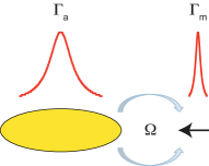
Fig.  9: A quantum emitter (black arrow) coupled to an optical antenna (gold spheroid) in the cavity QED picture. $\Gamma_{\mathrm{a}}$ and $\Gamma_{\mathrm{m}}$ respectively represent the antenna and the emitter resonance linewidths, with $\Gamma_{\mathrm{a}}\gg\Gamma_{\mathrm{m}}$. The interaction strength between the two systems is parametrized by the Rabi frequency $\Omega$.

3.2.2 Antenna efficiency.  

We now derive the relevant antenna parameters starting from $\eta_{\mathrm{a}}$. As discussed in Section 2, $\eta_{\mathrm{a}}$ depends on the antenna as well as on the position and orientation of the emitter. To avoid details a good approximation for $\eta_{\mathrm{a}}$ is the ratio between the scattering and the extinction cross sections of the antenna. This definition should not be considered a crude approximation, but rather an upper bound that is very close to the realistic values obtained for high-performance antennas.⁷⁹ Using Eq. (28) we arrive at

$$\eta_{\mathrm{a}}=\dfrac{1}{1+\dfrac{\gamma}{\omega_{\mathrm{p}}}\dfrac{9\sqrt{\epsilon_{\mathrm{b}}L}\,\mathrm{AR}^{2}}{2(ka)^{3}}}.$$ (29)

Equation (29) shows that $\eta_{\mathrm{a}}$ decreases quite rapidly with the antenna volume, whereas the dependence on material losses enters through the quantity $\gamma/\omega_{\mathrm{p}}$.¹⁰⁹ Table 1 displays this parameter for selected metals. Note, however, that these values are for a static electric field.

Table 1: Tabulated values of $\gamma/\omega_{\mathrm{p}}$ for selected metals.¹⁰⁹ Lowering the temperature $T$ reduces the absorption losses by an amount that is different for each metal.

Material	$T=273K$	$T=77K$
Au	0.0024	0.0006
Ag	0.0018	0.00036
Al	0.0051	0.00063
Cu	0.0022	0.00029

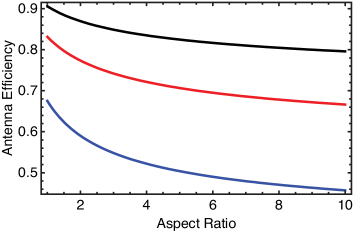
Fig.  10: Antenna efficiency as a function of AR plotted for three different values of $ka$: 0.5 (black), 0.4 (red), 0.3 (blue). $\gamma/\omega_{\mathrm{p}}=0.005$ for all curves.

Figure 10 plots $\eta_{\mathrm{a}}$ as a function AR for different values of $ka$. For a resonance wavelength of 600 nm, $ka=0.5$ corresponds to an optical antenna with linear dimensions of the order of 100 nm. Moreover, we choose $\gamma/\omega_{\mathrm{p}}=0.005$ and $\epsilon_{\mathrm{b}}=1$ to reproduce the performances presented in Ref. ³⁶. As expected, $\eta_{\mathrm{a}}$ decreases with AR and with $ka$. Nonetheless, for $ka\simeq 0.5$ $\eta_{\mathrm{a}}$ is large in a wide range of aspect ratios.

3.2.3 $Q$ factor.  

The $Q$ factor can be easily obtained from the formula $Q=\omega_{o}/\Gamma_{\mathrm{a}}$.⁶⁴ Adding $\eta_{\mathrm{a}}$ leads to

$$Q=\eta_{\mathrm{a}}\dfrac{9L\,\mathrm{AR}^{2}}{2(ka)^{3}}.$$ (30)

Figure 11 displays the $Q$ factor as a function of AR and $ka$. Note the competition between the decrease of $\eta_{\mathrm{a}}$ in Fig. 10 and the increase of the $Q$ factor with AR. For $ka\ll 1$ absorption losses dominate and the $Q$ factor saturates to the value $Q=(\omega_{\mathrm{p}}/\gamma)\sqrt{L/\epsilon_{\mathrm{b}}}$.

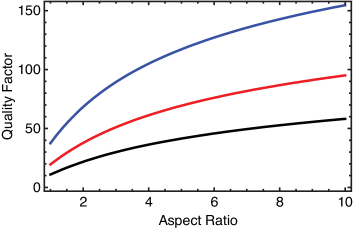
Fig.  11: $Q$ factor as a function of AR plotted for three different values of $ka$: 0.5 (black), 0.4 (red), 0.3 (blue). $\gamma/\omega_{\mathrm{p}}=0.005$ for all curves.

3.2.4 Field enhancement.  

For the calculation of $K$ we consider the antenna apex. We start from Eq. (18) and replace $\xi$ and $E_{\mathrm{dip}}$ with the values obtained from Eq. (28). The lighting-rod effect reads $\xi=3AR^{2}(1-L)/2$ and $E_{\mathrm{dip}}=2\alpha E_{o}/a^{3}$. A few algebraic operations lead to

$$K=\left(\dfrac{9}{2}\eta_{\mathrm{a}}\dfrac{\mathrm{AR}^{2}}{(ka)^{3}}\right)^{2}(1-L)^{2}.$$ (31)

Note that the $(ka)^{-6}$ dependence is compensated by a drop in $\eta_{\mathrm{a}}$. In fact, when $ka$ approaches zero, $K$ saturates to the value

$$\lim_{ka\to 0}K=\left(\dfrac{\omega_{\mathrm{p}}}{\gamma}\right)^{2}\dfrac{(1-L)^{2}}{\epsilon_{\mathrm{b}}L},$$ (32)

which depends on the material losses and the antenna geometry. Indeed, Fig. 12 indicates that $K$ falls off when $\gamma/\omega_{\mathrm{p}}$ increases.

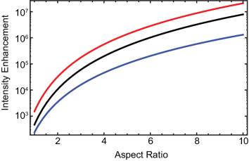
Fig.  12: Intensity enhancement as a function of AR plotted for different values of $ka$ and $\gamma/\omega_{\mathrm{p}}$: $ka=0.5$ and $\gamma/\omega_{\mathrm{p}}=0.005$ (black), $ka=0.4$ and $\gamma/\omega_{\mathrm{p}}=0.005$ (red), $ka=0.4$ and $\gamma/\omega_{\mathrm{p}}=0.05$ (blue).

3.2.5 Optical antennas are electrically small.  

The inset in Fig. 13 depicts a nanospheroid and an infinitesimal dipole antenna enclosed in the Chu virtual sphere of radius $r$. We also consider a nanosphere and an ideal electrically small antenna. The $Q$ factor for these radiating systems is plotted in Fig. 13 as a function of $kr$. According to the Chu theory, a metal nanosphere should be an efficient electrically small antenna, because it can fill the virtual sphere. Indeed the $Q$ factor of a nanosphere agrees very well with the result of Eq. (25) when $kr<1$. However, for $kr\ll 1$ the curve saturates to $\omega_{\mathrm{p}}/(\sqrt{3}\gamma)$. When the nanosphere is replaced by a nanospheroid the $Q$ factor increases, because the available radiating volume is not fully exploited.

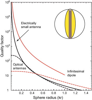
Fig.  13: $Q$ factor as a function of $kr$ for an ideal electrically small antenna (black solid curve), an infinitesimal dipole (red solid curve), and optical antennas (dashed curves): a nanosphere (black) and a nanospheroid (red). We choose $\gamma/\omega_{\mathrm{p}}=0.003$ for the nanosphere, AR=3 and $\gamma/\omega_{\mathrm{p}}=0.05$ for the nanospheroid, and $r/a=50$ for the infinitesimal dipole. The inset shows an infinitesimal dipole (brown) and a nanospheroid (yellow) enclosed in the radiating sphere.

In summary, metal nanoparticles are electrically small antennas, agree with the Chu theory and share the resulting limitations. These turn out to be very important for optical antennas, because the fact that the $Q$ factor and the reactive energy increase when the antenna volume decreases may be exploited to enhance light-matter interactions.

3.3 Comparison with optical resonators

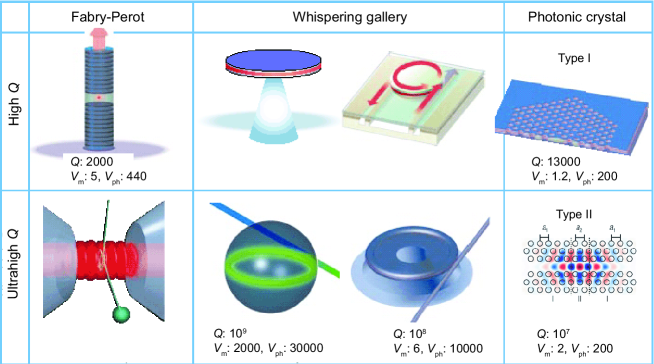
Fig.  14: Figures of merit for optical resonators: $Q$ factor, mode volume $V_{\mathrm{m}}$ and physical volume $V_{\mathrm{ph}}$. $V_{\mathrm{m}}$ and $V_{\mathrm{ph}}$ are both in units of the cubic wavelength. Figure adapted with permission from Macmillan Publishers Ltd: Nature (Ref. ¹⁸), copyright (2003) and Nat. Mater (Ref. ²¹), copyright (2005).

We are ready to compare the figures of merit of optical antennas with those of optical microcavities. For our purpose we choose the following cavity parameters: radiation efficiency, $Q$ factor, mode volume and footprint. The latter represents the actual device volume $V_{\mathrm{ph}}$. Literature values for these quantities are indicated in Fig. 14 with the corresponding resonator models.^{18, 21}

3.3.1 Antenna efficiency.  

For a more direct comparison with optical resonators, we use $V_{\mathrm{ph}}$ in units of $(\lambda/n_{\mathrm{b}})^{3}$ to obtain

$$\eta_{\mathrm{a}}=\dfrac{1}{1+\dfrac{\gamma}{\omega_{\mathrm{p}}}\dfrac{3}{4\pi^{2}}\dfrac{\sqrt{\epsilon_{\mathrm{b}}L}}{V_{\mathrm{ph}}}}.$$ (33)

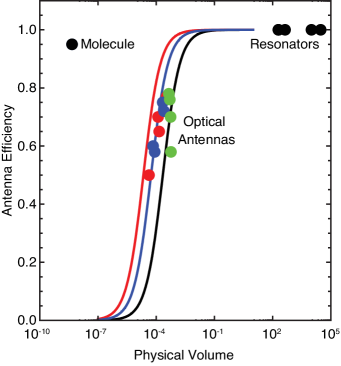
Fig.  15: Antenna efficiency as a function of $V_{\mathrm{ph}}$. The curves represent the antenna model: AR=1, $\gamma/\omega_{\mathrm{p}}=0.005$ (black), AR=10, $\gamma/\omega_{\mathrm{p}}=0.005$ (blue), AR=1, $\gamma/\omega_{\mathrm{p}}=0.0005$ (red). The circles refer to resonators, a molecule and optical antennas:³⁶ nanospheroids (green), nanorods (red), and nanorod pairs (blue).

The curves plotted in Fig. 15 correspond to different values of $\gamma/\omega_{\mathrm{p}}$ and AR (see the figure caption for details). It is shown that $\eta_{\mathrm{a}}$ drops when $V_{\mathrm{ph}}$ is smaller than about 10^-4 cubic wavelengths, a value that strongly depends on $\gamma/\omega_{\mathrm{p}}$. On top of these curves the filled circles refer to antenna designs discussed in Ref. ³⁶, namely nanospheroids (green), nanorods (red) and nanorod pairs (blue). The data agree well with our model. The dependence of $\eta_{\mathrm{a}}$ on $V_{\mathrm{ph}}$ illustrates the competition between absorption and radiation losses and recalls the conflict with the enhancement of light-matter interaction, which requires an optical antenna with a strong reactive behavior. For the sake of comparison, we also indicate $V_{\mathrm{ph}}$ and $\eta_{\mathrm{a}}$ for optical resonators and a molecule with $\eta_{o}\simeq 1$.

3.3.2 $Q$ factor.  

The $Q$ factor is inversely proportional to $V_{\mathrm{ph}}$ and Eq. (30) can be rewritten as

$$Q=\eta_{\mathrm{a}}\dfrac{3}{4\pi^{2}}\dfrac{L}{V_{\mathrm{ph}}}$$ (34)

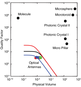
Fig.  16: $Q$ factor as a function of $V_{\mathrm{ph}}$. The curves represent the antenna model: AR=1, $\gamma/\omega_{\mathrm{p}}=0.005$ (black), AR=10, $\gamma/\omega_{\mathrm{p}}=0.005$ (blue), AR=1, $\gamma/\omega_{\mathrm{p}}=0.0005$ (red). The filled circles refer to resonators, a molecule and optical antennas:³⁶ nanospheroids (green), nanorods (red), and nanorod pairs (blue).

Figure 16 compares Eq. (34) with the antenna designs of Ref. ³⁶, as well as with selected optical resonators and a single molecule. The $Q$ factor of optical antennas is much smaller than in the other systems and for very small values of $V_{\mathrm{ph}}$ it is determined by the absorption losses and the antenna geometry. Since the response time is proportional to the $Q$ factor, optical antennas might represent a unique opportunity for enhancing light-matter interaction and, at the same time, meet the requirements of ultrafast optics. For example, a single molecule or ultrahigh-$Q$ cavities have response times of the order of nanoseconds. Resonators with a high $Q$ factor can cope with picosecond pulses. Optical antennas may offer the possibility of working with femtosecond pulses. In this respect, an important point of concern is whether antennas could increase light-matter interaction as much as optical resonators.

3.3.3 Spontaneous emission rate.  

The enhancement of the SE rate is obtained from Eq. (19) upon replacing $K$ with the expression given in Eq. (31). A few more algebraic steps lead to

$$\dfrac{\Gamma_{\mathrm{t}}}{\Gamma_{o}}=\eta_{\mathrm{a}}\dfrac{9}{16\pi^{4}}\dfrac{(1-L)^{2}}{V_{\mathrm{ph}}^{2}}.$$ (35)

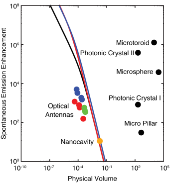
Fig.  17: Enhancement of the SE rate as a function of $V_{\mathrm{ph}}$. The curves represent the antenna model: AR=1, $\gamma/\omega_{\mathrm{p}}=0.005$ (black), AR=10, $\gamma/\omega_{\mathrm{p}}=0.005$ (blue), AR=1, $\gamma/\omega_{\mathrm{p}}=0.0005$ (red). The filled circles refer to resonators, a nanocavity²⁶ and optical antennas:³⁶ nanospheroids (green), nanorods (red), and nanorod pairs (blue).

Figure 17 demonstrates that the Purcell factor of optical resonators and the modification of the SE rate by optical antennas can be of the same order of magnitude. Furthermore, it is shown that the designs discussed in Ref. ³⁶ can compete with the performances of high-$Q$ photonic-crystal cavities

3.3.4 Mode volume.  

The last topic to be discussed is the mode volume. We point out that $V_{\mathrm{m}}$ is not a well defined quantity for optical antennas, because a dissipative environment does not have normalizable true modes.¹¹⁰ Since we are mostly interested in presenting figures of merit and scaling laws, we are satisfied with a definition of $V_{\mathrm{m}}$ based on Eq. (11). We thus write

$$V_{\mathrm{m}}=\dfrac{3}{4\pi^{2}}Q\left(\dfrac{\Gamma_{\mathrm{t}}}{\Gamma_{o}}\right)^{-1}.$$ (36)

We then replace the $Q$ factor and the enhancement of the SE rate using Eqs. (34) and (35), respectively, to arrive at

$$V_{\mathrm{m}}=\dfrac{L}{(1-L)^{2}}V_{\mathrm{ph}}.$$ (37)

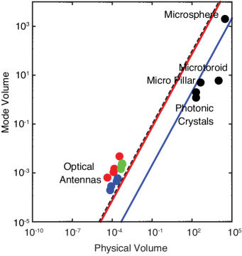
Fig.  18: Mode volume as a function of $V_{\mathrm{ph}}$. The curves represent the antenna model: AR=1, $\gamma/\omega_{\mathrm{p}}=0.005$ (black), AR=10, $\gamma/\omega_{\mathrm{p}}=0.005$ (blue), AR=1, $\gamma/\omega_{\mathrm{p}}=0.0005$ (red). The filled circles refer to resonators and optical antennas:³⁶ nanospheroids (green), nanorods (red), and nanorod pairs (blue). The dashed line marks $V_{\mathrm{m}}=V_{\mathrm{ph}}$.

Figure 18 compares the result of Eq. (37) with the mode volume of optical resonators. Note that even for the smallest photonic-crystal cavities $V_{\mathrm{m}}$ is about three orders of magnitude larger than for optical antennas. Furthermore, while for the latter $V_{\mathrm{m}}$ is comparable to $V_{\mathrm{ph}}$, for microcavities $V_{\mathrm{ph}}$ is significantly larger than $V_{\mathrm{m}}$.

An alternative way to derive $V_{\mathrm{m}}$ for an optical antenna utilizes the vacuum Rabi frequency $\Omega$. The latter can be obtained from a Green-function formulation of QED.^{104, 105} If the antenna leads to a strong modification of the SE rate ($\Gamma_{\mathrm{t}}/\Gamma_{o}\gg 1$), we can ignore the free-space radiation modes and approximate the imaginary part of the Green function with a Lorentzian of width $\Gamma_{\mathrm{a}}$. It can be shown that the Rabi frequency is related to $\Gamma_{\mathrm{t}}$ and $\Gamma_{\mathrm{a}}$ through the formula

$$\Omega=\sqrt{\dfrac{\Gamma_{\mathrm{t}}\Gamma_{\mathrm{a}}}{4}}.$$ (38)

From Eqs. (28) and (35) we find

$$\Omega=\dfrac{1-L}{\sqrt{L}}\dfrac{1}{\sqrt{V_{\mathrm{ph}}}},$$ (39)

Note that the above expression is given in units of $\omega^{2}d/(4\sqrt{\epsilon_{0}\hbar\pi^{3}c^{3}})$. Since $\Omega=\sqrt{\omega_{o}d^{2}/(2\epsilon_{0}\hbar V_{\mu})}$, where $V_{\mu}$ is the mode volume in dimensional units, one obtains the same result of Eq. (37).

After these considerations, we once more wish to discuss the competition between $\eta_{\mathrm{a}}$ and the enhancement of light-matter interaction. While $\eta_{\mathrm{a}}$ drops very rapidly when the antenna dimensions become smaller than a certain value that primarily depends on the parameter $\gamma/\omega_{\mathrm{p}}$, the enhancement of the SE rate increases and, despite the low $Q$ factor, it reaches values that compete with those of state-of-the-art optical cavities. Within these opposite trends there is a parameter range where optical antennas could function as nanoscale resonators with a tiny device footprint (see Fig. 19), manageable absorption losses and ultrafast operation.

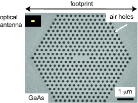
Fig.  19: Device footprint for a GaAs photonic-crystal cavity (figure adapted with permission from Ref. ¹³⁷. Copyright (2007) by SPIE) and an optical antenna.

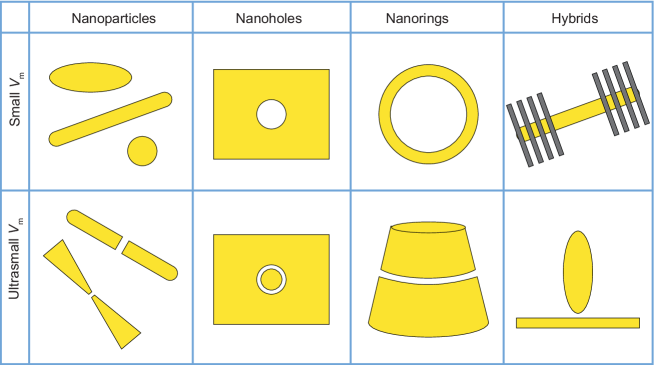
Fig.  20: Classification of optical antennas according to their mode volume $V_{\mathrm{m}}$ and confinement method, namely nanoparticles,^{16, 34, 36} nanoholes and nanocavities,^{138, 25, 26, 27} nanorings^{139, 102} and hybrid approaches. ^{144, 140, 141, 142, 143} Nanoholes and nanocavities may be understood as the complementary structure of metal nanoparticles. Nanorings and nanodisks of deep subwavelength dimensions should be considered as nanoparticles. Otherwise they correspond to whispering gallery resonators. Hybrid approaches range from the combination of nanoscale structures with optical microcavities (upper panel) to the exploitation of near-field effects with non-resonant geometries like a metal film (bottom panel). Note that sorting based on the $Q$ factor, as in Fig. 14, would be less meaningful.

We based our discussion on a simplified antenna model, which is nevertheless able to relate the main physical magnitudes of a resonator with those of an antenna and provide scaling laws for the figures of merit. Moreover, we have found good agreement between the outcome of our model and realistic antenna designs ³⁶. These are indicated as filled circles in the previous figures. Although we based the analysis on metal nanoparticles, we wish to point out that our expressions are in principle applicable to a larger class of antennas and nanocavities, since the geometrical factor $L$ is the only quantity that depends on the specific design. This is confirmed in Fig. 17, where we show that the parameters of a nanocavity fit our model very well.

Inspired by Fig. 14, we wish to conclude our analysis by presenting in Fig. 20 a classification of optical antennas according to their mode volume and confinement method. In doing so we keep in mind that this field is still making rapid progress. Our attempt is thus to indicate which approaches are consolidating and how they may differ from conventional strategies that have been used in the past century to confine light at optical frequencies. The striking differences with respect to Fig. 14 must not only be attributed to the role of SPP resonances, but also to the different level of theory involved in the resonator design. In fact, while optical microcavities rely on physical optics, nanoscale cavities owe their properties to near-field optics, whose wealth of effects may lead to unprecendented possibilities in the resonator design.^{111, 112}

4 Conclusions and outlook

We investigated fluorescence enhancement by optical antennas. Previous works indicated that at optical wavelengths losses by real metals could quench light emission. We established that this is not a fundamental constraint and showed that the interaction can be improved by more than three orders of magnitude without substantial quenching.³⁴

We took advantage of computational nano-optics to analyze the significant role that geometrical details play in determining the antenna behavior.^{36, 38} Moreover, we discussed the choice of different metals to enhance emitters from the ultraviolet to the near-infrared spectral range.³⁷ We would like to emphasize that these performances occur for distances such that microscopic effects can be safely neglected^{113, 114, 115} and our design strategies are solely based on electrodynamics considerations like for radio-wave antennas.⁶³

Optical antennas that strongly enhance the SE rate may improve the quantum yield of weak emitters, such as silicon nano-crystals,¹¹⁶ molecules,¹¹⁷ nanotubes⁸⁵ or diamond color centers,¹¹⁸ and provide a handle on photophysical processes in general.^{77, 119} Furthermore, a larger decay rate permits a higher degree of light emission, with immediate implications for single-photon sources.^{120, 121}

An important theme of our research has been the enhancement of light-matter interaction towards levels pertaining to optical resonators. To better understand the implications of these findings, we derived figures of merit using antenna theory³⁹ and compared them to common resonator designs.^{18, 21} Despite absorption losses we found that antennas are promising candidates for implementing the functionalities of optical resonators at the nanoscale. Moreover, having a low $Q$ factor, antennas do not suffer from the bandwidth limitations that are common to high-finesse cavities.

Altogether, these settings hold great promise for interfacing photons to a quantum system beyond the framework of cavity QED¹⁷ and urge further thorough theoretical and experimental investigations. These include studying the quantum optical phenomena that take place when an optical antenna mediates the interaction between photons and single quantum emitters in the full QED picture and beyond continuous wave excitation.³³ For instance, a number of proposals for quantum information science that are based on cavity-assisted interactions could be explored in this way.^{122, 123}

The ultrafast response of optical antennas, combined with their ability to funnel light beyond the diffraction limit with a high throughput,⁵² has immediate implications for scanning implementations of time-resolved, multidimensional and nonlinear nanoscopies.^{124, 125, 126, 127, 128, 129} Furthermore, combining ultrafast spectroscopy, field-enhanced spectroscopy and quantum optics could push forward the possibility of the coherent optical access of a quantum emitter above cryogenic temperatures,^{130, 131} and monitor quantum coherence under conditions where dephasing processes occur at very short time scales.^{132, 133}

The stringent requirements on photon management imposed by quantum-optical applications might turn out to be extremely useful also for classical information processing to achieve, for instance, nonlinearities at the single-photon level.¹³⁴ In both cases we have to fight the mismatch between light and nanoscale matter to attain strong and controllable interactions; we need to process very small optical signals, ideally down to single photons and possibly at very high rates. Thus, studying the physics and engineering of optical antennas may also pave the way to the next generation of nanophotonics devices.^{135, 136}

References

- Grober et al. 1997 R. D. Grober, R. J. Schoelkopf and D. E. Prober, Appl. Phys. Lett., 1997, 70, 1354–1356.
- Pohl 2000 D. Pohl, in Near-field Optics: Principles and Applications, ed. M. Ohtsu and X. Zhu, World Scientific Publ., Singapore, 2000, ch. Near-field optics seen as an antenna problem, pp. 9–21.
- Mühlschlegel et al. 2005 P. Mühlschlegel, H.-J. Eisler, O. J. F. Martin, B. Hecht and D. W. Pohl, Science, 2005, 308, 1607–1609.
- Schuck et al. 2005 P. J. Schuck, D. P. Fromm, A. Sundaramurthy, G. S. Kino and W. E. Moerner, Phys. Rev. Lett., 2005, 94, 017402.
- Bharadwaj et al. 2009 P. Bharadwaj, B. Deutsch and L. Novotny, Adv. Opt. Photon., 2009, 1, 438–483.
- Anker et al. 2008 J. N. Anker, W. P. Hall, O. Lyandres, N. C. Shah, J. Zhao and R. P. V. Duyne, Nat. Mater., 2008, 7, 442–453.
- Schuller et al. 2010 J. A. Schuller, E. S. Barnard, W. Cai, Y. C. Jun, J. S. White and M. L. Brongersma, Nat. Mater., 2010, 9, 193–204.
- Novotny and van Hulst 2011 L. Novotny and N. van Hulst, Nat. Photon., 2011, 5, 83–90.
- Biagioni et al. 2011 P. Biagioni, J.-S. Huang and B. Hecht, ArXiv e-prints, 2011.
- Giannini et al. 2011 V. Giannini, A. I. Fernández-Domínguez, S. C. Heck and S. A. Maier, Chem. Rev., 2011, 111, 3888–3912.
- Mayer and Hafner 2011 K. M. Mayer and J. H. Hafner, Chem. Rev., 2011, 111, 3828–3857.
- Greffet 2005 J.-J. Greffet, Science, 2005, 308, 1561–1563.
- Drexhage 1974 K. Drexhage, Prog. Opt., North-Holland, Amsterdam, 1974, vol. 12, pp. 164–232.
- Chance et al. 1978 R. Chance, A. Prock and R. Silbey, Adv. Chem. Phys., 1978, 37, 1–65.
- Metiu 1984 H. Metiu, Prog. Surf. Sci., 1984, 17, 153–320.
- Moskovits 1985 M. Moskovits, Rev. Mod. Phys., 1985, 57, 783–826.
- Haroche and Kleppner 1989 S. Haroche and D. Kleppner, Phys. Today, 1989, 42, 24–30.
- Vahala 2003 K. J. Vahala, Nature, 2003, 424, 839–846.
- Benisty et al. 1999 Confined Photon Systems: Fundamentals and Applications, ed. H. Benisty, J.-M. Gérard, R. Houdré, J. Rarity and C. Weisbuch, Springer Verlag, Berlin, New York, 1999.
- Akahane et al. 2003 Y. Akahane, T. Asano, B.-S. Song and S. Noda, Nature, 2003, 425, 944–947.
- Song et al. 2005 B.-S. Song, S. Noda, T. Asano and Y. Akahane, Nat. Mater., 2005, 4, 207–210.
- Hill et al. 2007 M. T. Hill, Y.-S. Oei, B. Smalbrugge, Y. Zhu, T. de Vries, P. J. van Veldhoven, F. W. M. van Otten, T. J. Eijkemans, J. P. Turkiewicz, H. de Waardt, E. J. Geluk, S.-H. Kwon, Y.-H. Lee, R. Notzel and M. K. Smit, Nat. Photon., 2007, 1, 589–594.
- Oulton et al. 2009 R. F. Oulton, V. J. Sorger, T. Zentgraf, R.-M. Ma, C. Gladden, L. Dai, G. Bartal and X. Zhang, Nature, 2009, 461, 629–632.
- Zhu et al. 2011 X. Zhu, J. Zhang, J. Xu and D. Yu, Nano Lett., 2011, 11, 1117–1121.
- Kroekenstoel et al. 2009 E. J. A. Kroekenstoel, E. Verhagen, R. J. Walters, L. Kuipers and A. Polman, Appl. Phys. Lett., 2009, 95, 263106.
- Maksymov et al. 2010 I. S. Maksymov, M. Besbes, J. P. Hugonin, J. Yang, A. Beveratos, I. Sagnes, I. Robert-Philip and P. Lalanne, Phys. Rev. Lett., 2010, 105, 180502.
- Bulu et al. 2011 I. Bulu, T. Babinec, B. Hausmann, J. T. Choy and M. Lončar, Opt. Express, 2011, 19, 5268–5276.
- Bergman and Stockman 2003 D. J. Bergman and M. I. Stockman, Phys. Rev. Lett., 2003, 90, 027402.
- Protsenko et al. 2005 I. E. Protsenko, A. V. Uskov, O. A. Zaimidoroga, V. N. Samoilov and E. P. O’Reilly, Phys. Rev. A, 2005, 71, 063812.
- Noginov et al. 2009 M. A. Noginov, G. Zhu, A. M. Belgrave, R. Bakker, V. M. Shalaev, E. E. Narimanov, S. Stout, E. Herz, T. Suteewong and U. Wiesner, Nature, 2009, 460, 1110–1112.
- Stockman 2010 M. I. Stockman, J. Opt., 2010, 12, 024004.
- Savasta et al. 2010 S. Savasta, R. Saija, A. Ridolfo, O. Di Stefano, P. Denti and F. Borghese, ACS Nano, 2010, 4, 6369–6376.
- Ridolfo et al. 2010 A. Ridolfo, O. Di Stefano, N. Fina, R. Saija and S. Savasta, Phys. Rev. Lett., 2010, 105, 263601.
- Rogobete et al. 2007 L. Rogobete, F. Kaminski, M. Agio and V. Sandoghdar, Opt. Lett., 2007, 32, 1623–1625.
- Agio et al. 2007 M. Agio, G. Mori, F. Kaminski, L. Rogobete, S. Kühn, V. Callegari, P. M. Nellen, F. Robin, Y. Ekinci, U. Sennhauser, H. Jäckel, H. H. Solak and V. Sandoghdar, SPIE, Proc., 2007, 6717, 67170R.
- Mohammadi et al. 2008 A. Mohammadi, V. Sandoghdar and M. Agio, New J. Phys., 2008, 10, 105015 (14pp).
- Mohammadi et al. 2009 A. Mohammadi, V. Sandoghdar and M. Agio, J. Comput. Theor. Nanosci., 2009, 6, 2024–2030.
- Mohammadi et al. 2010 A. Mohammadi, F. Kaminski, V. Sandoghdar and M. Agio, J. Phys. Chem. C, 2010, 114, 7372–7377.
- Hansen 1981 R. C. Hansen, IEEE, Proc., 1981, 69, 170–182.
- Zewail 2000 A. H. Zewail, J. Phys. Chem. A, 2000, 104, 5660–5694.
- Rabitz et al. 2000 H. Rabitz, R. de Vivie-Riedle, M. Motzkus and K. Kompa, Science, 2000, 288, 824–828.
- Gersten and Nitzan 1980 J. Gersten and A. Nitzan, J. Chem. Phys., 1980, 73, 3023–3037.
- Gersten and Nitzan 1981 J. Gersten and A. Nitzan, J. Chem. Phys., 1981, 75, 1139–1152.
- Ruppin 1982 R. Ruppin, J. Chem. Phys., 1982, 76, 1681–1684.
- Bohren and Huffman 1983 C. F. Bohren and D. R. Huffman, Absorption and Scattering of Light by Small Particles, John Wiley & Sons, New York, 1983.
- Barnes et al. 2003 W. L. Barnes, A. Dereux and T. W. Ebbesen, Nature, 2003, 424, 824–830.
- Johnson and Christy 1972 P. B. Johnson and R. W. Christy, Phys. Rev. B, 1972, 6, 4370–4379.
- Kreibig 2008 U. Kreibig, Appl. Phys. B, 2008, 93, 79–89.
- Mojarad et al. 2008 N. M. Mojarad, V. Sandoghdar and M. Agio, J. Opt. Soc. Am. B, 2008, 25, 651–658.
- Mojarad and Agio 2009 N. M. Mojarad and M. Agio, Opt. Express, 2009, 17, 117–122.
- Chen et al. 2009 X.-W. Chen, V. Sandoghdar and M. Agio, Nano Lett., 2009, 9, 3756–3761.
- Chen et al. 2010 X.-W. Chen, V. Sandoghdar and M. Agio, Opt. Express, 2010, 18, 10878–10887.
- Novotny 2007 L. Novotny, Phys. Rev. Lett., 2007, 98, 266802.
- Alù and Engheta 2008 A. Alù and N. Engheta, Phys. Rev. Lett., 2008, 101, 043901.
- Greffet et al. 2010 J.-J. Greffet, M. Laroche and F. Marquier, Phys. Rev. Lett., 2010, 105, 117701.
- Meystre and Sargent III 2007 P. Meystre and M. Sargent III, Elements of Quantum Optics, Springer, Berlin, Heidelberg, 4th edn, 2007.
- Taminiau et al. 2008 T. H. Taminiau, F. D. Stefani, F. B. Segerink and N. F. van Hulst, Nat. Photon., 2008, 2, 234–237.
- Curto et al. 2010 A. G. Curto, G. Volpe, T. H. Taminiau, M. P. Kreuzer, R. Quidant and N. F. van Hulst, Science, 2010, 329, 930–933.
- Li et al. 2007 J. Li, A. Salandrino and N. Engheta, Phys. Rev. B, 2007, 76, 245403.
- Hofmann et al. 2007 H. F. Hofmann, T. Kosako and Y. Kadoya, New J. Phys., 2007, 9, 217.
- Kühn et al. 2008 S. Kühn, G. Mori, M. Agio and V. Sandoghdar, Mol. Phys., 2008, 106, 893–908.
- Kosako et al. 2010 T. Kosako, Y. Kadoya and H. F. Hofmann, Nat. Photon., 2010, 4, 312–315.
- Balanis 2005 C. A. Balanis, Antenna Theory, John Wiley & Sons, Hoboken, NJ, 3rd edn, 2005.
- Jackson 1999 J. D. Jackson, Classical Electrodynamics, John Wiley & Sons, New York, 3rd edn, 1999.
- Aravind et al. 1981 P. Aravind, A. Nitzan and H. Metiu, Surf. Sci., 1981, 110, 189–204.
- Wokaun et al. 1982 A. Wokaun, J. P. Gordon and P. F. Liao, Phys. Rev. Lett., 1982, 48, 957–960.
- Cline et al. 1986 M. P. Cline, P. W. Barber and R. K. Chang, J. Opt. Soc. Am. B, 1986, 3, 15–21.
- Zeman and Schatz 1987 E. J. Zeman and G. C. Schatz, J. Phys. Chem., 1987, 91, 634–643.
- Girard and Dereux 1996 C. Girard and A. Dereux, Rep. Prog. Phys., 1996, 59, 657–699.
- Purcell 1946 E. Purcell, Phys. Rev., 1946, 69, 681.
- Wylie and Sipe 1984 J. M. Wylie and J. E. Sipe, Phys. Rev. A, 1984, 30, 1185–1193.
- Xu et al. 2000 Y. Xu, R. K. Lee and A. Yariv, Phys. Rev. A, 2000, 61, 033807.
- Taminiau et al. 2008 T. H. Taminiau, F. D. Stefani and N. F. van Hulst, Opt. Express, 2008, 16, 10858–10866.
- Blanco and García de Abajo 2004 L. A. Blanco and F. J. García de Abajo, Phys. Rev. B, 2004, 69, 205414.
- Kaminski et al. 2007 F. Kaminski, V. Sandoghdar and M. Agio, J. Comput. Theor. Nanosci., 2007, 4, 635–643.
- Lakowicz 2005 J. R. Lakowicz, Analytical Biochem., 2005, 337, 171–194.
- Nitzan and Brus 1981 A. Nitzan and L. E. Brus, J. Chem. Phys., 1981, 75, 2205–2214.
- Mertens et al. 2007 H. Mertens, A. F. Koenderink and A. Polman, Phys. Rev. B, 2007, 76, 115123.
- Mohammadi et al. 2009 A. Mohammadi, F. Kaminski, V. Sandoghdar and M. Agio, Intl. J. Nanotechnology, 2009, 6, 902–914.
- Lide 2006 CRC Handbook of Chemistry and Physics, ed. D. R. Lide, CRC Press, Boca Raton, FL, 87th edn, 2006.
- Wokaun et al. 1983 A. Wokaun, H.-P. Lutz, A. P. King, U. P. Wild and R. R. Ernst, J. Chem. Phys., 1983, 79, 509–514.
- Kühn et al. 2006 S. Kühn, U. Håkanson, L. Rogobete and V. Sandoghdar, Phys. Rev. Lett., 2006, 97, 017402.
- Anger et al. 2006 P. Anger, P. Bharadwaj and L. Novotny, Phys. Rev. Lett., 2006, 96, 113002.
- Beveratos et al. 2001 A. Beveratos, R. Brouri, T. Gacoin, J.-P. Poizat and P. Grangier, Phys. Rev. A, 2001, 64, 061802.
- O’Connell et al. 2002 M. J. O’Connell, S. M. Bachilo, C. B. Huffman, V. C. Moore, M. S. Strano, E. H. Haroz, K. L. Rialon, P. J. Boul, W. H. Noon, C. Kittrell, J. Ma, R. H. Hauge, R. B. Weisman and R. E. Smalley, Science, 2002, 297, 593–596.
- Pavesi and Turan 2010 Silicon Nanocrystals, ed. L. Pavesi and R. Turan, Wiley-VCH, Weinheim, 2010.
- Klimov 2010 Nanocrystal Quantum Dots, ed. V. Klimov, CRC Press, Boca Raton, FL, 2010.
- Klimov et al. 2002 V. Klimov, M. Ducloy and V. Letokhov, Eur. Phys. J. D, 2002, 20, 133–148.
- Aizpurua et al. 2005 J. Aizpurua, G. W. Bryant, L. J. Richter, F. J. García de Abajo, B. K. Kelley and T. Mallouk, Phys. Rev. B, 2005, 71, 235420.
- Goncharenko et al. 2006 A. V. Goncharenko, M. M. Dvoynenko, H.-C. Chang and J.-K. Wang, Appl. Phys. Lett., 2006, 88, 104101.
- Goncharenko et al. 2007 A. Goncharenko, H.-C. Chang and J.-K. Wang, Ultramicroscopy, 2007, 107, 151–157.
- Tilaki et al. 2007 R. Tilaki, A. Iraji zad and S. Mahdavi, Appl. Phys. A, 2007, 88, 415–419.
- Ekinci et al. 2008 Y. Ekinci, H. H. Solak and J. F. Löffler, J. Appl. Phys., 2008, 104, 083107.
- Langhammer et al. 2008 C. Langhammer, M. Schwind, B. Kasemo and I. Zorić, Nano Lett., 2008, 8, 1461–1471.
- Chowdhury et al. 2009 M. H. Chowdhury, K. Ray, S. K. Gray, J. Pond and J. R. Lakowicz, Analytical Chem., 2009, 81, 1397–1403.
- Chan et al. 2008 G. H. Chan, J. Zhao, G. C. Schatz and R. P. V. Duyne, J. Phys. Chem. C, 2008, 112, 13958–13963.
- Pakizeh et al. 2009 T. Pakizeh, C. Langhammer, I. Zorić, P. Apell and M. Käll, Nano Lett., 2009, 9, 882–886.
- Palik and Ghosh 1998 Handbook of Optical Constants of Solids, ed. E. D. Palik and G. Ghosh, Academic Press, 1998.
- Ray et al. 2007 K. Ray, M. H. Chowdhury and J. R. Lakowicz, Anal. Chem., 2007, 79, 6480–6487.
- Oulton et al. 2008 R. F. Oulton, G. Bartal, D. F. P. Pile and X. Zhang, New J. Phys., 2008, 10, 105018.
- Koenderink 2010 A. F. Koenderink, Opt. Lett., 2010, 35, 4208–4210.
- Kuttge et al. 2010 M. Kuttge, F. J. García de Abajo and A. Polman, Nano Lett., 2010, 10, 1537–1541.
- Maier 2006 S. A. Maier, Opt. Express, 2006, 14, 1957–1964.
- Wylie 1986 J. Wylie, PhD thesis, University of Toronto, Canada, 1986.
- Knöll et al. 2001 L. Knöll, S. Scheel and D.-G. Welsch, in Coherence and Statistics of Photons and Atoms, ed. J. Perina, Wiley, New York, 2001, ch. QED in dispersing and absorbing dielectric media, pp. 1–60.
- Trügler and Hohenester 2008 A. Trügler and U. Hohenester, Phys. Rev. B, 2008, 77, 115403.
- Chu 1948 L. J. Chu, J. Appl. Phys., 1948, 19, 1163–1175.
- McLean 1996 J. S. McLean, Antennas Propag., IEEE Trans., 1996, 44, 672–676.
- Ashcroft and Mermin 1976 N. W. Ashcroft and N. D. Mermin, Solid State Physics, Saunders College Publishing, Fort Worth, 1976.
- Dutra and Nienhuis 2000 S. M. Dutra and G. Nienhuis, Phys. Rev. A, 2000, 62, 063805.
- Luk’yanchuk et al. 2010 B. Luk’yanchuk, N. I. Zheludev, S. A. Maier, N. J. Halas, P. Nordlander, H. Giessen and C. T. Chong, Nat. Mater., 2010, 9, 707–715.
- Halas et al. 2011 N. J. Halas, S. Lal, W.-S. Chang, S. Link and P. Nordlander, Chem. Rev., 2011, 111, 3913–3961.
- Persson 1978 B. N. J. Persson, J. Phys. C, 1978, 11, 4251–4269.
- Ford and Weber 1984 G. W. Ford and W. H. Weber, Phys. Rep., 1984, 113, 195–287.
- Leung 1990 P. T. Leung, Phys. Rev. B, 1990, 42, 7622–7625.
- Biteen et al. 2005 J. S. Biteen, D. Pacifici, N. S. Lewis and H. A. Atwater, Nano Lett., 2005, 5, 1768–1773.
- Kinkhabwala et al. 2009 A. Kinkhabwala, Z. Yu, S. Fan, Y. Avlasevich, K. Müllen and W. E. Moerner, Nat. Photon., 2009, 3, 654–657.
- Turukhin et al. 1996 A. V. Turukhin, C.-H. Liu, A. A. Gorokhovsky, R. R. Alfano and W. Phillips, Phys. Rev. B, 1996, 54, 16448–16451.
- Mackowski et al. 2008 S. Mackowski, S. Wörmke, A. J. Maier, T. H. P. Brotosudarmo, H. Harutyunyan, A. Hartschuh, A. O. Govorov, H. Scheer and C. Bräuchle, Nano Lett., 2008, 8, 558–564.
- Lounis and Orrit 2005 B. Lounis and M. Orrit, Rep. Prog. Phys., 2005, 68, 1129.
- Schietinger et al. 2009 S. Schietinger, M. Barth, T. Aichele and O. Benson, Nano Lett., 2009, 9, 1694–1698.
- Turchette et al. 1995 Q. A. Turchette, C. J. Hood, W. Lange, H. Mabuchi and H. J. Kimble, Phys. Rev. Lett., 1995, 75, 4710–4713.
- van Loock et al. 2006 P. van Loock, T. D. Ladd, K. Sanaka, F. Yamaguchi, K. Nemoto, W. J. Munro and Y. Yamamoto, Phys. Rev. Lett., 2006, 96, 240501.
- Sánchez et al. 1999 E. J. Sánchez, L. Novotny and X. S. Xie, Phys. Rev. Lett., 1999, 82, 4014–4017.
- Mukamel 1999 S. Mukamel, Principles of Nonlinear Optical Spectroscopy, Oxford Univ. Press, New York, 1999.
- Guenther et al. 2002 T. Guenther, C. Lienau, T. Elsaesser, M. Glanemann, V. M. Axt, T. Kuhn, S. Eshlaghi and A. D. Wieck, Phys. Rev. Lett., 2002, 89, 057401.
- Ichimura et al. 2004 T. Ichimura, N. Hayazawa, M. Hashimoto, Y. Inouye and S. Kawata, Phys. Rev. Lett., 2004, 92, 220801.
- Hartschuh 2008 A. Hartschuh, Angew. Chem. Int. Ed., 2008, 47, 8178–8191.
- Abramavicius et al. 2009 D. Abramavicius, B. Palmieri, D. V. Voronine, F. Šanda and S. Mukamel, Chem. Rev., 2009, 109, 2350–2408.
- Brinks et al. 2010 D. Brinks, F. D. Stefani, F. Kulzer, R. Hildner, T. H. Taminiau, Y. Avlasevich, K. Mullen and N. F. van Hulst, Nature, 2010, 465, 905–908.
- Hildner et al. 2011 R. Hildner, D. Brinks and N. F. van Hulst, Nat. Phys., 2011, 7, 172–177.
- Engel et al. 2007 G. S. Engel, T. R. Calhoun, E. L. Read, T.-K. Ahn, T. Mancal, Y.-C. Cheng, R. E. Blankenship and G. R. Fleming, Nature, 2007, 446, 782–786.
- Panitchayangkoon et al. 2010 G. Panitchayangkoon, D. Hayes, K. A. Fransted, J. R. Caram, E. Harel, J. Wen, R. E. Blankenship and G. S. Engel, Proc. Natl. Acad. Sci., 2010, 107, 12766–12770.
- Chang et al. 2007 D. E. Chang, A. S. Sørensen, E. A. Demler and M. D. Lukin, Nat. Phys., 2007, 3, 807–812.
- Miller 1989 D. A. B. Miller, Opt. Lett., 1989, 14, 146–148.
- Miller 2009 D. A. B. Miller, IEEE, Proc., 2009, 97, 1166–1185.
- Nomura et al. 2007 M. Nomura, S. Iwamoto and Y. Arakawa, SPIE Newsroom, 2007.
- Genet and Ebbesen 2007 C. Genet and T. W. Ebbesen, Nature, 2007, 445, 39–46.
- Aizpurua et al. 2003 J. Aizpurua, P. Hanarp, D. S. Sutherland, M. Käll, G. W. Bryant and F. J. García de Abajo, Phys. Rev. Lett., 2003, 90, 057401.
- Barth et al. 2010 M. Barth, S. Schietinger, S. Fischer, J. Becker, N. Nüsse, T. Aichele, B. Löchel, C. Sönnichsen and O. Benson, Nano Lett., 2010, 10, 891–895.
- Snapp et al. 2010 N. Snapp, C. Yu, D. Englund, F. Koppens, M. Lukin and H. Park, APS Meeting Abstracts, 2010, 14003–+.
- Eghlidi et al. 2009 H. Eghlidi, K. G. Lee, X.-W. Chen, S. Götzinger and V. Sandoghdar, Nano Lett., 2009, 9, 4007–4011.
- Devilez et al. 2010 A. Devilez, B. Stout and N. Bonod, ACS Nano, 2010, 4, 3390–3396.
- Le et al. 2005 F. Le, N. Z. Lwin, J. M. Steele, M. Käll, N. J. Halas and P. Nordlander, Nano Lett., 2005, 5, 2009–2013.