Curvaton Reheating and Intermediate Inflation in Brane Cosmology

Abstract

In this paper, we study the curvaton reheating mechanism for an intermediate inflationary universe in brane world cosmology. In contrast to our previous work, we assume that when the universe enters the kination era, it is still in the high-energy regime. We then discuss, in detail, the new cosmological constraints on both the model parameters and the physical quantities.

I Introduction

Inflation as the most promising framework for understanding the physics of the very early universe, relates the universe evolution to the properties of one or more scalar inflaton fields that is responsible for creating universe acceleration. This in turn causes a flat and homogeneous universe which later evolves into the present structure. Furthermore, inflation can be a solution to many other cosmological issues such as horizon and flatness problems Tzirakis –Guth . The inflationary universe model may also provide a causal explanation of the origin of the observed anisotropy of the cosmic microwave background radiation (CMBR), and also large scale structures distribution Albrecht –Hinshaw .

In intermediate inflation, the scale factor of the universe in a certain extend intermediate between a power law and exponential expansion whereas the expansion rate is faster than power law and slower than exponential ones. In this kind, the slow-roll approximation conditions are satisfied with time and thus same as in power-law inflation case, within the model, there is no natural end to inflation Rendall –Liddle . While during the inflationary period the universe becomes dominated by the inflation scalar potential, at the end of inflation the universe represents a combination of kinetic and potential energies related to the scalar field, which is assumed to take place at very low temperatureRandall –Campuzano .

In the standard reheating mechanism after inflation while the temperature grows in many orders of magnitude, most of the matter and radiation of the universe was created via the decay of the inflaton field and the Big-Bang universe is recovered. The reheating temperature is particularly very important to cosmologists. In the standard mechanism of reheating, in the stage of oscillation of the scalar field a minimum in the inflaton potential is something crucial for the reheating mechanism Kofman –del .

However, since the scalar field potential in some models does not present a minimum, the conventional mechanism, offered to bring inflation to an end, becomes ineffective. These models are well known as non-oscillating or simply NO Models. To overcome this shortcoming, a scalar field, dubbed curvaton is represented in the mechanism of reheating in these kind of models Mollerach –Lyth . The curvaton scenario is suggested as an alternative to produce the primordial scalar perturbation where in turn is responsible for the structure formation. When it decay into conventional matter, it creates an efficient mechanism of reheating. The energy density of carvaton field is not diluted during inflation therefore the curvaton may be responsible for some or all the matter content of the universe at the present time Papantonopoulos ; Campuzano .

In the Randall-Sundrum cosmology, the issue of inflation of a single brane in an AdS bulk successfully consolidates the idea that universe is in a three-dimensional brane within a higher-dimensional bulk spacetime. In the high energy limit, the brane inflationary models contain correction terms in their Friedmann equations with significant consequences in the inflationary dynamics Binetruy –Shir . In this work, in the context of brane intermediate inflationary cosmology, we would like to introduce the curvaton field as a mechanism to bring inflation to an end. A similar approach to study the subject has been investigated in del and Lopez . The authors in del , employs curvaton scenario for intermediate inflationary models in standard cosmology whereas in Lopez , the steep inflation model in brane cosmology has been studied with the curvaton field responsible to bring inflation to an end. Here, in an attempt to integrate the above two works, curvaton reheating and intermediate inflation in brane cosmological models has been investigated with the aim to explore the dynamics of the universe within and after inflation era. In lowenergy , we assumed that when the universe enters the kination era, it is in the low energy regime. Here, in both inflationary and kination epochs the universe is in high energy regime. The model then suggests new constraints on the space parameters and predict reheating temperature in different scenarios.

II The Model

In this section, a five-dimensional brane cosmology is studied with the modified Friedmann equation given by Shiromizu ; Kamenshchik ,

$$H^{2}=\kappa\rho_{\phi}[1+\frac{\rho_{\phi}}{2\lambda}]+\frac{\Lambda_{4}}{3}+\frac{\xi}{a^{4}},$$ (1)

where $H=\dot{a}/a$ is the Hubble parameter. The $\rho_{\phi}$ and $\Lambda_{4}$ are,respectively, the matter field confined to the brane and the four-dimensional cosmological constant. we also assume that $\kappa=8\pi G/3=8\pi/(3m_{p}^{2})$. The influence of the bulk gravitons on the brane is shown in the last term of the equation, where $\xi$ is integration constant. The four and five-dimensional Planck masses are related through brane tension $\lambda$ in $m_{p}=\sqrt{3M_{5}^{6}/(4\pi\lambda)}$, where constrained by nucleosynthesis. The brane tension satisfies the inequality $\lambda>(1MeV)^{4}$. In the following, in the inflation epoch, we assume that the universe is in the high energy regime, i.e. $\rho_{\phi}\gg\lambda$. We suppose that the four-dimensional cosmological constant is vanished. In addition, at the beginning of inflation, the last term in (1) vanishes and, thus we are left with the effective Friedmann equation given by

$$H^{2}\simeq\beta\rho_{\phi}^{2},$$ (2)

where $\beta$ is equal to $\kappa/(2\lambda)$, with the dimension of $m_{p}^{-6}$. Furthermore, we assume that the inflaton field is bounded to the brane, therefore its field equation is in the form of:

$$\ddot{\phi}+3H\dot{\phi}+V^{\prime}=0.$$ (3)

In the above equation, $V(\phi)$ is the effective scalar potential. The dot and prime respectively represent derivative with respect to the cosmological time and scalar field $\phi$. We also have the conservation equation as

$$\dot{\rho_{\phi}}+3H(\rho_{\phi}+p_{\phi})=0,$$ (4)

where the energy density and pressure respectively are given by $\rho_{\phi}=(\dot{\phi}^{2}/2)+V(\phi)$, and $p_{\phi}=(\dot{\phi}^{2}/2)-V(\phi)$. For convenience, we also take units in which $c={\hbar}=1$.

In intermediate inflationary scenarios, one can find the exact solution by taking the scale factor $a(t)$ as

$$a(t)=\exp(At^{f}),$$ (5)

where the power $f$ is a parameter limited as $0<f<1$, and the coefficient $A$ is a positive constant with dimension $m_{P}^{f}$.

From equations (2), (3) and (5), one can find potential $V(\phi)$ and scalar field $\phi(t)$ as

$$V(\phi)={\frac{2(1-f)}{9\beta}}[6fA{(\frac{3\beta^{1/2}}{4(1-f)})^{f}}\phi^{2(f-1)}-\frac{(1-f)}{\phi^{2}}],$$ (6)

and

$$\phi(t)=[{\frac{4(1-f)}{3\beta^{1/2}}}t]^{1/2}.$$ (7)

Therefore, we obtain the Hubble parameter in terms of inflaton scalar field $\phi$ as

$$H(\phi)=fA(\frac{3\beta^{1/2}}{4(1-f)})^{f-1}\phi^{-2(1-f)}.$$ (8)

By solving the field equations in slow roll approximation, with simple power law scalar potential in the form of

$$V(\phi)=fA\beta^{(f-2)/2}[\frac{3}{4(1-f)}]^{f-1}\phi^{-2(1-f)},$$ (9)

One can find scale factor sam as in equation (5). With the potential (9) in the slow roll approximation we find solutions for $\phi(t)$ and $H(\phi)$. these solutions are similar to those obtained in the exact solution and expressed by (7) and (8). It is notable that no extreme point can be found for these potentials.

In our model, the dimensionless slow roll parameters $\varepsilon\simeq V^{\prime 2}/(3\beta V^{3})$ and $\eta\simeq V^{\prime\prime}/(3\beta V^{2})$, respectively, become

$$\varepsilon\simeq\frac{4(1-f)^{2}}{3fA\beta^{f/2}[\frac{3}{4(1-f)}]^{f-1}}\phi^{-2f},$$ (10)

and

$$\eta\simeq\frac{2(1-f)(3-2f)}{3fA\beta^{f/2}[\frac{3}{4(1-f)}]^{f-1}}\phi^{-2f}.$$ (11)

Note that for $0<f<1$, the ratio $\varepsilon/\eta=2(1-f)/(3-2f)$ is less than one. Moreover, $\eta$ earlier than $\varepsilon$ reaches unity. As a result, the end of inflation is controlled by the condition $\eta=1$ instead of $\varepsilon=1$. We also find the inflaton field at the end of inflation as

$$\phi_{e}=[\frac{2(1-f)(3-2f)}{3fA\beta^{f/2}[\frac{3}{4(1-f)}]^{f-1}}]^{1/2f},$$ (12)

where the subscript $"e"$ is used to indicate end of inflationary period.

III The Curvaton Field Constraint During The Kinetic Epoch

With disregarding the term $V^{\prime}$ in equation (3) compare to the friction term $3H\dot{\phi}$, the model enters a new era called the kinetic epoch or kination. From now on, we use the subscript (or superscript) $"k"$, to mark quantities at the beginning of this period. During the kination era we have $\dot{\phi}^{2}/2>V(\phi)$ which could be seen as a stiff fluid, since $p_{\phi}=\rho_{\phi}$. Since we assume that the universe in the kinetic epoch is still in high energy regime, the field equations (1) and (3) become, $H^{2}=\beta\dot{\phi}^{4}/4$ and $\ddot{\phi}+3H\dot{\phi}=0$, where the second equation gives

$$\dot{\phi}={\dot{\phi}}_{k}(\frac{a_{k}}{a})^{3}.$$ (13)

Therefore, energy density and Hubble parameter in terms of scale factor respectively become

$$\rho_{\phi}(a)=\rho_{\phi}^{k}(\frac{a_{k}}{a})^{6},$$ (14)

and

$$H(a)=H_{k}(\frac{a_{k}}{a})^{6}.$$ (15)

In the above equations the ”k” label is associated to the inflaton field at the beginning of the kinetic era.

With the curvaton field complying the Klein-Gordon equation, we assume that the scalar potential associated to the curvaton is given by $U(\sigma)=m^{2}\sigma^{2}/2$, with $m$ to be curvaton mass.

In comparison with the curvaton energy density, let us consider that $\rho_{\phi}$ is dominant component. Further, assume that curvaton field oscillates around minimum of its effective potential. During kination era, the curvaton density evolves as a non-relativistic matter, i.e. $\rho_{\sigma}\propto a^{-3}$ and inflaton stays dominated. Therefore, by decay of the the curvaton field into radiation, the Big-Bang cosmology is recovered.

In the inflation epoch, the curvaton field is assumed to be effectively massless. Therefore, the curvaton rolls down its potential until its kinetic energy is weakened by exponential expansion and then almost vanishes. As a result the curvaon field becomes frozen roughly to a constant value, $\sigma_{\ast}\approx\sigma_{e}$. The subscript $"\ast"$ denotes the period when the cosmological scale exits the horizon.

We also assume that during kination era, the Hubble parameter value decreases and become equal to the curvaton mass, i.e. $m\simeq H$. Then, at this point, curvaton field becomes effectively massive and from equation (15), we get

$$\frac{m}{H_{k}}=(\frac{a_{k}}{a_{m}})^{6},$$ (16)

where the subscript $"m"$ marks quantities during kination at the time when the curvaton mass $m$ has order of $H$.

To prohibit a period of curvaton-driven inflation, the inflaton domination must still hold, i.e. $\rho_{\phi}^{m}\gg\rho_{\sigma}$($\sim U(\sigma_{e})\simeq U(\sigma_{\ast}))$. This inequality gives us a constraint on the values of the curvaton field $\sigma_{\ast}$. When $H\simeq m$,then, we get $\frac{m^{2}\sigma_{\ast}^{2}}{2\rho_{\phi}^{m}}\ll 1$, meaning that the curvaton field $\sigma_{\ast}$ satisfies the constraint

$$\sigma_{\ast}^{2}\ll\frac{2}{m\beta^{1/2}}\cdot$$ (17)

the ratio of the potential energies at the end of inflation, becomes

$$\frac{U_{e}}{V_{e}}=\frac{m^{2}\sigma_{\ast}^{2}\beta^{1/2}}{2H_{e}}<1,$$ (18)

and, therefore, curvaton energy sub dominated. The curvaton mass then should obey the constraint

$$m^{2}<H_{e}^{2}=(fA)^{2/f}(\frac{3-2f}{2})^{2(f-1)/f}.$$ (19)

The above constraint imposed by the fact that the curvaton field during the inflationary era must be effectively massless and therefore we have $m<H_{e}$. When curvaton field mass becomes important, i.e. $m\simeq H$, its energy density decays same as a non-relativistic matter as $\rho_{\sigma}=m^{2}\sigma_{\ast}^{2}a_{m}^{3}/(2a^{3})$. In fact whenever curvaton undergoes quasi-harmonic oscillations, the potential and kinetic energy densities become comparable.

In general, the curvaton field decay happens in two different scenarios. When the curvaton field first dominates the cosmic expansion and then decays. Or its decay occurs before its domination. Next section we discusses these scenarios in more details.

IV Constraints on model parameters

Case 1: Curvaton decay after domination

If the curvaton field dominates the cosmic expansion (i.e. $\rho_{\sigma}>\rho_{\phi}$), then, at a distance, let us assume that, when $a=a_{eq}$, the inflaton and curvaton energy densities become equal. Therefore, from equations (14) and (15), by using $\rho_{\sigma}\propto a^{-3}$, we obtain

$$(\frac{\rho_{\sigma}}{\rho_{\phi}})|_{a=a_{eq}}=\frac{\beta^{1/2}m^{2}\sigma_{\ast}^{2}}{2}\frac{a_{m}^{3}}{a_{k}^{6}}\frac{a_{eq}^{3}}{H_{k}}=1.$$ (20)

Using (15), (16) and (20), the Hubble parameter, $H_{eq}$, in terms of the curvaton parameters can be obtained

$$H_{eq}=H_{k}(\frac{a_{k}}{a_{eq}})^{6}=\beta m^{3}\sigma_{\ast}^{4}/4.$$ (21)

The decay parameter $\Gamma_{\sigma}$ is bounded by nucleosynthesis, so the curvaton field must decay before nucleosynthesis which means that $H_{nucl}\sim 10^{-40}<\Gamma_{\sigma}$ (in units of Planck mass $m_{p}$). From $\Gamma_{\sigma}<H_{eq}$, we obtain a constraint on $\Gamma_{\sigma}$, as

$$10^{-40}<\Gamma_{\sigma}<\beta m^{3}\sigma_{\ast}^{4}/4.$$ (22)

Following the argument given in del , by studying the scalar perturbations related to the curvaton field $\sigma$, we find new constraints on our model parameters. When the curvaton field decays, the Bardeen parameter, $P_{\zeta}$, whose observed value is about $2.4\times 10^{-9}$ Komatsu , becomes Lyth

$$P_{\zeta}\simeq\frac{1}{9\pi^{2}}\frac{H_{\ast}^{2}}{\sigma_{\ast}^{2}}\cdot$$ (23)

With regards to $\sigma_{\ast}^{2}\gg H_{\ast}^{2}/(4\pi^{2})$, the spectrum of fluctuations is automatically gaussian and $\Gamma_{\sigma}$ independent, thus, one can ease the analysis of space parameter. From expressions (8), (12) and (23), we may write

$$A=[\frac{9\pi^{2}\sigma_{\ast}^{2}P_{\zeta}}{f^{2}}(\frac{3-2f}{2f}-N_{\ast})^{\frac{2(1-f)}{f}}]^{f/2},$$ (24)

where

$$N_{\ast}=\int_{t_{\ast}}^{t_{e}}{H(t^{\prime})dt^{\prime}}=A[\frac{3\beta^{1/2}}{4(1-f)}]^{f}(\phi_{e}^{2f}-\phi_{\ast}^{2f}).$$ (25)

Equation (25) defines number of e-folds corresponding to the cosmological scales, i.e. the number of remaining inflationary e-folds at the time when the cosmological scale exits the horizon. Then, the constraint given by equation (19) changes to

$$m^{2}<9\pi^{2}\sigma_{\ast}^{2}P_{\zeta}(1-\frac{2fN_{\ast}}{3-2f})^{2(1-f)/f}.$$ (26)

By using equations (22) and (26) we obtain an upper limit on $\Gamma_{\sigma}$ as

$$\Gamma_{\sigma}<\frac{27\pi^{3}}{4}\beta\sigma_{\ast}^{7}P_{\zeta}^{3/2}(1-\frac{2fN_{\ast}}{3-2f})^{3(1-f)/f}.$$ (27)

Moreover, by using Big Bang Nucleosynthesis $(BBN)$ temperature, $T_{BBN}$, we give the constraints for our model parameters $A$ and $f$. The reheating temperature is given by $T_{BBN}\sim 10^{-22}$ (in unit of $m_{p}$). Since the reheating temperature occurs before the $BBN$, $T_{reh}>T_{BBN}$, by knowing that $T_{reh}\sim\Gamma_{\sigma}^{1/2}>T_{BBN}$ one obtains the following constraints,

$$H_{\ast}^{2}=f^{2}A^{2/f}[\frac{3-2f}{2f}-N_{\ast}]^{2(f-1)/f}>(36\pi^{2})^{4/7}(P_{\zeta}T_{BBN})^{4/7}\sim 10^{-16},$$ (28)

where for later consideration we have used the scalar spectral index $n_{s}$ closed to one and thus $m\approx H_{*}/10$ Sanchez .

By fitting equation (28) in its lower limit, Fig. 1 (left panel) shows contours of model parameters $f$ and $A$ corresponding to different number of e-folds, $N_{\ast}$. Similarly, Fig. 1 (right panel) shows the constraints when the upper limit, $H_{\ast}\leqslant 10^{-5}$ Dimopoulos , is used.

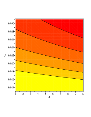
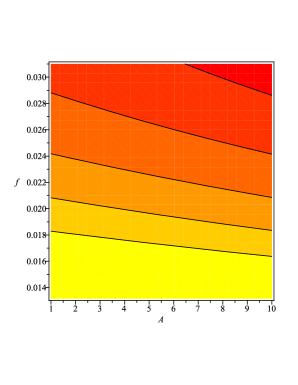
Figure 1: contour plot for the parameters $f$ and $A$ in both curvaton decay after and before domination, fitted from the lower limit of the $T_{BBN}$ (left panel) and upper limit of the $T_{BBN}$ (right panel). Lower values of the $N_{\ast}$ parameters correspond to darker regions and the contour levels are separated by the quantity $\bigtriangleup N_{\ast}=10$. Here, we have considered the values of $N_{\ast}$, from $40$ to $80$.

Case 2: Curvaton decay before domination

We assume that the curvaton decays before its energy density becomes greater than the inflaton energy density. Furthermore, the mass of the curvaton is considered toe comparable with the Hubble expansion rate, such that $\rho_{\sigma}\propto a^{-3}$. Following del , we also assume that the curvaton field decays when $\Gamma_{\sigma}=H(a_{d})=H_{d}$. Then, from equation (15) we obtain

$$\Gamma_{\sigma}=H_{d}=H_{k}(\frac{a_{k}}{a_{d}})^{6},$$ (29)

where ”d” stands for quantities when the curvaton decays.

By assuming that $\Gamma_{\sigma}<m$ and $\Gamma_{\sigma}>H_{eq}$), we yield,

$$\frac{\beta m^{2}\sigma_{\ast}^{4}}{4}<\frac{\Gamma_{\sigma}}{m}<1.$$ (30)

In this scenario, the Bardeen parameter becomes

$$P_{\zeta}\simeq\frac{r_{d}^{2}}{16\pi^{2}}\frac{H_{\ast}^{2}}{\sigma_{\ast}^{2}},$$ (31)

where $r_{d}=\frac{\rho_{\sigma}}{\rho_{\phi}}|_{a=a_{d}}$. Employing $\rho_{\sigma}=m^{2}\sigma_{\ast}^{2}a_{m}^{3}/(2a^{3})$ and simple algebraic manipulation in (14), (16) and (29) we get

$$r_{d}=\frac{\sigma_{\ast}^{2}}{2}(\frac{\beta m^{3}}{\Gamma_{\sigma}})^{1/2}.$$ (32)

From expressions (8), (12), (25), (31) and (32), one yields

$$A=[\frac{64\pi^{2}P_{\zeta}\Gamma_{\sigma}}{\beta m^{3}\sigma_{\ast}^{2}f^{2}}(\frac{3-2f}{2f}-N_{\ast})^{\frac{2(1-f)}{f}}]^{f/2}.$$ (33)

In addition, the constraint given by equation (19) becomes

$$m^{2}<\frac{64\pi^{2}P_{\zeta}\Gamma_{\sigma}}{\beta m^{3}\sigma_{\ast}^{2}}(1-\frac{2fN_{\ast}}{3-2f})^{2(1-f)/f}.$$ (34)

Now, by using equations (30) and (34), we could get the inequality

$$\Gamma_{\sigma}<\frac{64\pi^{2}P_{\zeta}}{\beta m^{3}\sigma_{\ast}^{2}}(1-\frac{2fN_{\ast}}{3-2f})^{2(1-f)/f},$$ (35)

which gives an upper limit on $\Gamma_{\sigma}$.

Finally, since the reheating temperature satisfies $T_{reh}>T_{BBN}$, and also $\Gamma_{\sigma}>T_{BBN}^{2}$, we obtain,

$$H_{\ast}^{2}=f^{2}A^{2/f}[\frac{3-2f}{2f}-N_{\ast}]^{2(f-1)/f}>(64\pi^{2})^{4/7}(P_{\zeta}T_{BBN})^{4/7}\sim 10^{-16},$$ (36)

where, as before, we have used the scalar spectral index $n_{s}$ closed to one. Note some similarities between (36) and (28), and therefore the same constraints on $A$ and $f$ for different number of e-folds can be considered in this case.

V Constraints on Curvaton Mass

By using tensor perturbations scheme, one can constrain the curvaton mass. From Kamenshchik , the gravitational wave amplitude is given by,

$$h_{GW}\simeq C_{1}H_{\ast},$$ (37)

where $C_{1}$ is a constant. If inflation occurs at an energy scale smaller than the grand unification, we have $H\ll 10^{-5}$, an advantage of curvaton approach over single inflaton field approach. Then, using $H_{\ast}^{2}=\beta V_{\ast}^{2}$, and (36) we find

$$h_{GW}^{2}\simeq C_{1}^{2}f^{2}A^{2/f}[\frac{3-2f}{2f}-N_{\ast}]^{2(f-1)/f}.$$ (38)

From equations (19) and (38), we yield the constraint

$$m^{2}<\frac{h_{GW}^{2}}{C_{1}^{2}}(\frac{3-2f-2fN_{\ast}}{3-2f})^{2(1-f)/f},$$ (39)

which gives an upper limit for the curvaton mass.

The authors in Langlois constrain the density fraction of the gravitational wave as

$$I\equiv h^{2}\int_{k_{BBN}}^{k_{\ast}}\Omega_{GW}(k)dlnk\simeq 2h^{2}\epsilon\Omega_{\gamma}(k_{0})h^{2}_{GW}(\frac{H_{\ast}}{\widetilde{H}})^{2/3}\leq 2\times 10^{-6},$$ (40)

where $k_{BBN}$ is physical momentum corresponding to the horizon at $BBN$. Also, $\Omega_{GW}(k)$ is density fraction of the gravitational wave as a function of $k$. At the present epoch we have $\Omega_{\gamma}(k_{0})=2.6\times 10^{-5}h^{-2}$, $\epsilon\sim 10^{-2}$ and $h=0.73$. Therefore, for the curvaton decay after or before domination, $\widetilde{H}$ is either $\widetilde{H}=H_{eq}$ or $\widetilde{H}=H_{d}$.

Case 1: Curvaton decay after domination

By using equations (21), (23) and (37), the constraint on (40) becomes

$$m^{3}\gtrsim 7.5\times 10^{-37}{P_{\zeta}}^{2}\sim 10^{-54}.$$ (41)

If the decay rate is of gravitational strength, then $\Gamma_{\sigma}\sim m^{3}$ Rodriguez –Lazarides and equation (22) imposes a third constraint as

$$\sigma_{\ast}^{4}>\frac{4}{\beta}\simeq 7.55\times 10^{-25}.$$ (42)

We also have two constraints (17) and (22). By using equations (19) and (23) for the curvaton decay after domination we find

$$\frac{m^{2}}{\sigma_{\ast}^{2}}<9\pi^{2}P_{\zeta}\sim 2.13\times 10^{-7}.$$ (43)

Therefore, for the curvaton decay after domination, we have five constraints (17), (22), (41)–(43) on $m$ or $\sigma_{\ast}$. Fig. 2 (left panel), shows the allowed region for curvaton mass in shaded color.

Case 2: Curvaton decay before domination

In this case, using the constraint on the density fraction of the gravitational wave, equation (40), and also using equations (29), (31) and (32), with regards to $\Gamma_{\sigma}^{1/2}>T_{BBN}$ we obtain

$$m^{3}\sigma_{\ast}^{2}\gtrsim 1.3\times 10^{-30}P_{\zeta}T_{BBN}\sim 10^{-61}.$$ (44)

By incorporating equations (30) and (44), a second constraint is given by Herrera

$$m^{2}>1.5\times 10^{-18}P_{\zeta}T_{BBN}\sim 10^{-49}.$$ (45)

By employing equation (30), a pair of new constraints can also be obtained as

$$m^{2}<1,$$ (46)

and

$$\sigma_{\ast}^{4}<7.55\times 10^{-25}.$$ (47)

Moreover, from equation (44) one can get a further constraint

$$m^{3/2}\sigma_{\ast}^{2}>\frac{7\times 10^{-6}P_{\zeta}}{\beta}\simeq 3.17\times 10^{-39}.$$ (48)

For curvaton decay before domination, we have the constraint (17). Further, from (19), (30), (31) and (32), a second constraint is

$$m^{4}\sigma_{\ast}^{2}<1.2\times 10^{-23}\pi^{2}P_{\zeta}\sim 2.9\times 10^{-31}.$$ (49)

Therefore, there are seven constraints (17), (44)–(49) on either $m$ or $\sigma_{\ast}$, for the curvaton decay before domination. In Fig. 2 (right panel), the shaded region shows the allowed region for $m$ which is bounded by the above constraints. Here, we have fixed the value of $\lambda$ (the tension of the brane) by $\lambda=7.9\times 10^{-25}$ (in units of $m_{p}$)Lopez .

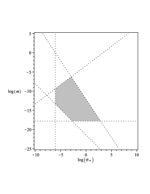
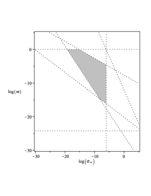
Figure 2: Allowed region of parameter space of the curvaton-brane intermediate inflation model for the case of curvaton domination after decay (left panel) and curvaton domination before decay (right panel). The allowed regions are shaded.

V.1 Constraint on the reheating temperature

As in Nojiri , the decay rate of curvaton field in some cases can be constrained by,

$$\Gamma_{\sigma}=g^{2}m,$$ (50)

where coupling of curvaton to its decay products is denoted by $g$. Therefore,

$$max(\frac{T_{BBN}}{m^{1/2}},m)\lesssim g\lesssim min(1,\frac{m\sigma^{3}}{T_{BBN}^{2}}),$$ (51)

is the allowed range for coupling constant. The inequality $m\lesssim g$ is caused by gravitational decay. In the case of curvaton decay before domination, by using $T_{reh}>T_{BBN}$, the constraint (51) represents an upper limit expressed by $g<m\sigma_{\ast}^{3}/T_{BBN}^{2}$. For the curvaton decay after domination, a lower limit is given by $T_{BBN}m^{-1/2}<g$.

Employing (51) and from Sanchez , knowing that $H_{\ast}\simeq 10^{-8}$, $\sigma_{\ast}\sim 10^{-3}$, $m\sim 10^{-9}$ (from $n_{s}\simeq 1$), then we get $10^{-9}\lesssim g\lesssim 1$. Also, from $T_{reh}\sim gm^{1/2}$, we have $10^{-27/2}\lesssim T_{reh}\lesssim 10^{-9/2}$ (in units of $m_{p}$)as the allowed range for the reheating temperature.

Alternatively, by choosing $\sigma_{\ast}=1$ Sanchez , from expression (51) the constraint on $g$ becomes $10^{-9}\lesssim g\lesssim 1$. Thus, from $T_{reh}\sim gm^{1/2}$, we have the same range for reheating temperature. Note also that the constraint on the density fraction of gravitational waves gives us $g\sim 1$ Sanchez . In this case, the reheating temperature becomes of the order of $T_{reh}\sim 10^{-9/2}$ (in units of $m_{p}$) which challenges gravitino constraint Dine .

VI Summary

In this paper, we investigated intermediate inflation in the brane-world cosmology when curavaton field is liable for universe reheating. We assumed that the universe in both inflationary and kination eras is in high energy regime which is strongly supported by the observation (for example see del ). In comparison to our previous work, lowenergy , where in the kination era the universe was considered to be in low energy regime, new constraints on the space and model parameters are obtained.

Following del , two cases have been considered in investigating universe reheating via curvaton mediation in brane cosmology; curvaton dominating the universe after or before its decay. As a result we have obtained an upper limit constrain on $\Gamma_{\sigma}$ expressed by equation (27) in the case of curvaton dominating the universe after it decays. As is given in equation (35) for the case after decay one obtains a lower limit constraint on $\Gamma_{\sigma}$. In the intermediate inflationary universe with the scale factor given by equation (5), there are two space parameters $A$ and $f$. In both scenarios, we have acquired constraints for the parameters expresses by equations (28) and (36). The contour plot of these parameters for different values of e-folding from both lower and upper limits of $T_{BBN}$ is also given in Fig. (1).

We constrained curvaton field and its mass in both cases. One, we obtained six constraints on pair ($m$, $\sigma_{\ast}$) by the region shown in Fig. 2 (left panel). Similarly, we found seven constraints on them, plotted in Fig. 2 (right panel). Finally, we explore the reheating scenario and from the result of previous sections, we find constraints on the reheating temperature.

References

- (1) H. Farajollahi, A. Ravanpak, Can. J. Phys. 88:939-945 (2010)
- (2) K. Tzirakis and W. H. Kinney, JCAP. 01, 028 (2009).
- (3) S. del Campo and R. Herrera, Phys. Lett. B670, 266-270 (2009).
- (4) A. Guth, Phys. Rev. D23, 347 (1981).
- (5) A. Albrecht and P. J. Steinhardt, Phys. Rev. Lett. 48, 1220 (1982).
- (6) J. Dunkley, E. Komatsu et al., Astrophys. J. Suppl. 180, 306-329 (2009).
- (7) G. Hinshaw, J. L. Weiland et al., Astrophys. J. Suppl. 180, 225-245 (2009).
- (8) A. D. Rendall, Class. Quant. Grav. 22, 1655-1666 (2005).
- (9) A. K. Sanyal, Adv. High Energy Phys. 2009, 630414 (2009).
- (10) J. D. Barrow, Phys. Lett. B235, 40 (1990).
- (11) A. G. Muslimov, Class. Quantum. Grav. 7, 231 (1990).
- (12) J. D. Barrow and A. R. Liddle, Phys. Rev. D47, 5219-5223 (1993).
- (13) L. Randall and R. Sundrum, Phys. Rev. Lett. 83, 3370-3373 (1999).
- (14) E. Papantonopoulos and V. Zamarias, JCAP. 0611, 005 (2006).
- (15) C. Campuzano, S. del Campo and R. Herrera, Phys. Rev. D72, 083515 (2005).
- (16) L. Kofman and A. Linde, JHEP. 0207, 004 (2002).
- (17) G. Felder, L. Kofman and A. Linde, Phys. Rev. D60, 103505 (1999).
- (18) S. del Campo and R. Herrera, Phys. Rev. D76, 103503 (2007).
- (19) S. Mollerach, Phys. Rev. D42, 313 (1990).
- (20) D. H. Lyth and D. Wands, Phys. Lett. B524, 5 (2002).
- (21) P. Binetruy, C. Deffayet and D. Langlois, Nucl. Phys. B. 565, 269 (2000).
- (22) P. Binetruy, C. Deffayet, U. Ellwanger and D. Langlois, Phys. Lett. B. 477, 285 (2000).
- (23) T. Shiromizu, K. Maeda and M. Sasaki, Phys. Rev. D. 62, 024012 (2000).
- (24) A. R. Liddle and L. A. Urena-Lopez, Phys. Rev. D68, 043517 (2003).
- (25) T. Shiromizu, K. Maeda and M. Sasaki, Phys. Rev. D62, 024012 (2000).
- (26) A. Kamenshchik, U. Moschella and V. Pasquier, Phys. Lett. B511, 265 (2001).
- (27) E. Komatsu et al.[WMAP Collaboration], Astrophys. J. Suppl. 180, 330 (2009).
- (28) J. C. Bueno Sanchez, K. Dimopoulos, JCAP. 0711, 007 (2007).
- (29) K. Dimopoulos and D. H. Lyth, Phys. Rev. D69, 123509 (2004).
- (30) D. Langlois, R. Maartens and D. Wands, Phys. Lett. B489, 259 (2000).
- (31) K. Dimopoulos, D. H. Lyth and Y. Rodriguez, JHEP. 0502, 055 (2005).
- (32) K. Dimopoulos, D. H. Lyth, A. Notari and A. Riotto, JHEP. 0307, 053 (2003).
- (33) K. Dimopoulos, Phys. Lett. B634, 331 (2006).
- (34) K. Dimopoulos, G. Lazarides, D. Lyth and R. Ruiz de Austri, Phys. Rev. D68, 123515 (2003).
- (35) C. Campuzano, S. del Campo, R. Herrera, E. Rojas and J. Saavedra, Phys. Rev. D80, 123531 (2009).
- (36) S. Nojiri, S. D. Odintsov and M. Sasaki, Phys. Rev. D71, 123509 (2004).
- (37) M. Dine, Cambridge University Press, First published in print format (2006).