Convergence of a Particle-based Approximation of the Block Online Expectation Maximization Algorithm

Abstract

Online variants of the Expectation Maximization (EM) algorithm have recently been proposed to perform parameter inference with large data sets or data streams, in independent latent models and in hidden Markov models. Nevertheless, the convergence properties of these algorithms remain an open problem at least in the hidden Markov case. This contribution deals with a new online EM algorithm which updates the parameter at some deterministic times. Some convergence results have been derived even in general latent models such as hidden Markov models. These properties rely on the assumption that some intermediate quantities are available in closed form or can be approximated by Monte Carlo methods when the Monte Carlo error vanishes rapidly enough. In this paper, we propose an algorithm which approximates these quantities using Sequential Monte Carlo methods. The convergence of this algorithm and of an averaged version is established and their performance is illustrated through Monte Carlo experiments.

 

This extended version of the paper “Convergence of a Particle-based Approximation of the Block Online Expectation Maximization Algorithm“, by S. Le Corff and G. Fort, provides detailed proofs which have been omitted in the submitted paper since they are very close to existing results. These additional proofs are postponed to Appendix B.

 

1 Introduction

The Expectation Maximization (EM) algorithm is a well-known iterative algorithm to solve maximum likelihood estimation in incomplete data models, see  [14]. Each iteration is decomposed into two steps: in the E-step the conditional expectation of the complete log-likelihood (log of the joint distribution of the hidden states and the observations) given the observations is computed; and the M-step updates the parameter estimate. The EM algorithm is mostly practicable if the model belongs to the curved exponential family, see [29, Section $1.5$] and [6, Section $10.1$], so that we assume below that our model belongs to this family. Under mild regularity conditions, this algorithm is known to converge to the stationary points of the log-likelihood of the observations, see [36]. However, the original EM algorithm cannot be used to perform online estimation or when the inference task relies on large data sets. Each iteration requires the whole data set and each piece of data needs to be stored and scanned to produce a new parameter estimate. Online variants of the EM algorithm were first proposed for independent and identically distributed (i.i.d.) observations: [5] proposed to replace the original E-step by a stochastic approximation using the new observation. Solutions have also been proposed in hidden Markov models (HMM):  [4] provides an algorithm for finite state-space HMM which relies on recursive computations of the filtering distributions combined with a stochastic approximation step. Note that, since the state-space is finite, deterministic approximations of these distributions are available. This algorithm has been extended to the case of general state-space models, the approximations of the filtering distributions being handled with Sequential Monte Carlo (SMC) algorithms, see [3], [10] and [25]. Unfortunately, it is quite challenging to address the asymptotic behavior of these algorithms (in the HMM case) since the recursive computation of the filtering distributions relies on approximations which are really difficult to control.

In [23], another online variant of the EM algorithm in HMM is proposed, called the Block Online EM (BOEM) algorithm. In this case, the data stream is decomposed into blocks of increasing sizes. Within each block, the parameter estimate is kept fixed and the update occurs at the end of the block. This update is based on a single scan of the observations, so that it is not required to store any block of observations. [23] provides results on the convergence and on the convergence rates of the BOEM algorithms. These analyses are established when the E-step (computed on each block) is available in closed form and when it can be approximated using Monte Carlo methods, under an assumption on the $\mathrm{L}_{p}$-error of the Monte Carlo approximation.

In this paper, we consider the case when the E-step of the BOEM algorithm is computed with SMC approximations: the filtering distributions are approximated using a set of random weighted particles, see [6] and [8]. The Monte Carlo approximation is based on an online variant of the Forward Filtering Backward Smoothing algorithm (FFBS) proposed in [4] and [10]. This method is appealing for two reasons: first, it can be implemented forwards in time i.e. within a block, each observation is scanned once and never stored and the approximation computed on each block does not require a backward step - this is crucial in our online estimation framework. Secondly, recent work on SMC approximations provides $\mathrm{L}_{p}$-mean control of the Monte Carlo error, see e.g. [19] and [9]. This control, combined with the results in [23], sparks off the convergence results and the convergence rates provided in this contribution.

The paper is organized as follows: our new algorithm called the Particle Block Online EM algorithm (P-BOEM) is derived in Section 2 together with an averaged version. Section 3 is devoted to practical applications: the P-BOEM algorithm is used to perform parameter inference in stochastic volatility models and in the more challenging framework of the Simultaneous Localization And Mapping problem (SLAM). The convergence properties and the convergence rates of the P-BOEM algorithms are given in Section 4.

2 The Particle Block Online EM algorithms

In Section 2.1, we fix notation that will be used throughout this paper. We then derive our online algorithms in Sections 2.2 and 2.3. We finally detail, in Section 2.4, the SMC procedure that makes our algorithm a true online algorithm.

2.1 Notations and Model assumptions

A hidden Markov model on $\mathbb{X}\times\mathbb{Y}$ is defined by an initial distribution $\chi$ on $(\mathbb{X},\mathcal{X})$ and two families of transition kernels. In this paper, the transition kernels are parametrized by $\theta\in\Theta$, where $\Theta\subseteq\mathbb{R}^{d_{\theta}}$ is a compact set. In the sequel, the initial distribution $\chi$ on $(\mathbb{X},\mathcal{X})$ is assumed to be known and fixed. The parameter is estimated online in the maximum likelihood sense using a sequence of observations $\mathbf{Y}$. Online maximum likelihood parameter inference algorithms were proposed either with a gradient approach or an EM approach. In the case of finite state-spaces HMM, [26] proposed a recursive maximum likelihood procedure. The asymptotic properties of this algorithm have recently been addressed in [34]. This algorithm has been adapted to general state-spaces HMM with SMC methods (see [18]). The main drawback of gradient methods is the necessity to scale the gradient components. As an alternative to performing online inference in HMM, online EM based algorithms have been proposed for finite state-spaces (see [4]) or general state-spaces HMM (see [3], [10] and [23]). [10] proposed a SMC method giving encouraging experimental results. Nevertheless, it relies on a combination of stochastic approximations and SMC computations so that its analysis is quite challenging. In [23], the convergence of an online EM based algorithm is established. This algorithm requires either the exact computation of intermediate quantities (available explicitly only in finite state-spaces HMM or in linear Gaussian models) or the use of Monte Carlo methods to approximate these quantities. We propose to apply this algorithm to general models where these quantities are replaced by SMC approximations. We prove that the Monte Carlo error is controlled in such a way that the convergence properties of [23] hold for the P-BOEM algorithms.

We now detail the model assumptions. Consider a family of transition kernels $\{m_{\theta}(x,x^{\prime})\mathrm{d}\lambda(x^{\prime})\}_{\theta\in\Theta}$ on $\mathbb{X}\times\mathcal{X}$, where $\mathbb{X}$ is a general state-space equipped with a countably generated $\sigma$-field $\mathcal{X}$, and $\lambda$ is a finite measure on $(\mathbb{X},\mathcal{X})$. Let $\{g_{\theta}(x,y)\mathrm{d}\nu(y)\}_{\theta\in\Theta}$ be a family of transition kernels on $\mathbb{X}\times\mathcal{Y}$, where $\mathbb{Y}$ is a general space endowed with a countably generated $\sigma$-field $\mathcal{Y}$ and $\nu$ is a measure on $(\mathbb{Y},\mathcal{Y})$. Let $\mathbf{Y}=\{\mathbf{Y}_{t}\}_{t\in\mathbb{Z}}$ be the observation process defined on $\left(\Omega,\mathbb{P},\mathcal{F}\right)$ and taking values in $\mathbb{Y}^{\mathbb{Z}}$. The batch EM algorithm is an offline maximum likelihood procedure which iteratively produces parameter estimates using the complete data log-likelihood (log of the joint distribution of the observations and the states) and a fixed set of observations, see [14]. In the HMM context presented above, given $T$ observations $\mathbf{Y}_{1:T}$, the missing data $x_{0:T}$ and a parameter $\theta$, the complete data log-likelihood may be written as (up to the initial distribution $\chi$ which is assumed to be known)

$$\ell_{\theta}(x_{0:T},\mathbf{Y}_{1:T})\stackrel{{\scriptstyle\mathrm{def}}}{{=}}\sum_{t=1}^{T}\left\{\log m_{\theta}(x_{t-1},x_{t})+\log g_{\theta}(x_{t},\mathbf{Y}_{t})\right\}\;,$$ (1)

where we use $x_{r:t}$ as a shorthand notation for the sequence $(x_{r},\dots,x_{t})$, $r\leq t$. Each iteration of the batch EM algorithm is decomposed into two steps. The E-step computes, for all $\theta\in\Theta,$ an expectation of the complete data log-likelihood under the conditional probability of the hidden states given the observations and the current parameter estimate $\hat{\theta}$. In the HMM context, due to the additive form of the complete data log-likelihood (1), the E-step is decomposed into $T$ expectations under the conditional probabilities $\Phi_{\hat{\theta},t,T}^{\chi,0}(\cdot,\mathbf{y})$ where

$$\Phi_{\theta,s,t}^{\chi,r}(h,\mathbf{y})\stackrel{{\scriptstyle\mathrm{def}}}{{=}}\frac{\int\chi(\mathrm{d}x_{r})\{\prod_{i=r}^{t-1}m_{\theta}(x_{i},x_{i+1})g_{\theta}(x_{i+1},\mathbf{y}_{i+1})\}\,h(x_{s-1},x_{s},\mathbf{y}_{s})\,\mathrm{d}\lambda(x_{r+1:t})}{\int\chi(\mathrm{d}x_{r})\{\prod_{i=r}^{t-1}m_{\theta}(x_{i},x_{i+1})g_{\theta}(x_{i+1},\mathbf{y}_{i+1})\}\,\mathrm{d}\lambda(x_{r+1:t})}\;,$$ (2)

for any bounded function $h$, any $\theta\in\Theta$, any $r<s\leq t$ and any sequence $\mathbf{y}\in\mathbb{Y}^{\mathbb{Z}}$. Then, given the current value of the parameter $\hat{\theta}$, the E-step amounts to computing the quantity

$$Q_{T}(\theta,\hat{\theta})\stackrel{{\scriptstyle\mathrm{def}}}{{=}}\frac{1}{T}\sum_{t=1}^{T}\Phi_{\hat{\theta},t,T}^{\chi,0}\left(\log m_{\theta}+\log g_{\theta},\mathbf{Y}\right)\;,$$ (3)

for any $\theta\in\Theta$. The M-step sets the new parameter estimate as a maximum of this expectation over $\theta$.

The computation of $\theta\mapsto Q_{T}(\theta,\hat{\theta})$ for any $\theta\in\Theta$ is usually intractable except in the case of complete data likelihood belonging to the curved exponential family, see [29, Section $1.5$] and [6, Section $10.1$]. Therefore, in the sequel, the following assumption is assumed to hold:

• 1. There exist continuous functions $\phi:\Theta\to\mathbb{R}$, $\psi:\Theta\to\mathbb{R}^{d}$ and $S:\mathbb{X}\times\mathbb{X}\times\mathbb{Y}\to\mathbb{R}^{d}$ s.t.

     $$\log m_{\theta}(x,x^{\prime})+\log g_{\theta}(x^{\prime},y)=\phi(\theta)+\left\langle S(x,x,^{\prime},y),\psi(\theta)\right\rangle\;,$$

     where $\left\langle\cdot,\cdot\right\rangle$ denotes the scalar product on $\mathbb{R}^{d}$.

  2. There exists an open subset $\mathcal{S}$ of $\mathbb{R}^{d}$ that contains the convex hull of $S(\mathbb{X}\times\mathbb{X}\times\mathbb{Y})$.

  3. There exists a continuous function $\bar{\theta}:\mathcal{S}\to\Theta$ s.t. for any $s\in\mathcal{S}$,

     $$\bar{\theta}(s)=\mathrm{argmax}_{\theta\in\Theta}\;\left\{\phi(\theta)+\left\langle s,\psi(\theta)\right\rangle\right\}\;.$$

Under AA1, the quantity $Q_{T}(\theta,\hat{\theta})$ defined by (3) becomes

$$Q_{T}(\theta,\hat{\theta})=\phi(\theta)+\left\langle\frac{1}{T}\sum_{t=1}^{T}\Phi_{\hat{\theta},t,T}^{\chi,0}\left(S,\mathbf{Y}\right),\psi(\theta)\right\rangle\;,$$ (4)

so that the definition of the function $\theta\mapsto Q_{T}(\theta,\hat{\theta})$ requires the computation of an expectation $\frac{1}{T}\sum_{t=1}^{T}\Phi_{\hat{\theta},t,T}^{\chi,0}\left(S,\mathbf{Y}\right)$ independently of $\theta$.

The M-step of the batch EM iteration amounts to computing

$$\bar{\theta}\left(\frac{1}{T}\sum_{t=1}^{T}\Phi_{\hat{\theta},t,T}^{\chi,0}\left(S,\mathbf{Y}\right)\right)\;.$$

This batch EM algorithm is designed for a fixed set of observations. A natural extension of this algorithm to the online context is to define a sequence of parameter estimates by

$$\theta_{t+1}=\mathrm{argmax}_{\theta}\ Q_{t+1}(\theta,\theta_{t})\;.$$

Unfortunately, the computation of $Q_{t+1}(\theta,\theta_{t})$ requires the whole set of observations to be stored and scanned for each estimation. For large data sets the computation cost of the E-step makes it intractable in this case. To overcome this difficulty, several online variants of the batch EM algorithm have been proposed, based on a recursive approximation of the function $\theta\mapsto Q_{t+1}(\cdot,\theta_{t})$ (see [3], [10] and [23]). In this paper, we focus on the Block Online EM (BOEM) algorithm, see [23].

2.2 Particle Block Online EM (P-BOEM)

The BOEM algorithm, introduced in [23], is an online variant of the EM algorithm. The observations are processed sequentially per block and the parameter estimate is updated at the end of each block. Let $\{\tau_{k}\}_{k\geq 1}$ be a sequence of positive integers denoting the length of the blocks and set

$$T_{n}\stackrel{{\scriptstyle\mathrm{def}}}{{=}}\sum_{k=1}^{n}\tau_{k}\quad\mbox{and}\quad T_{0}\stackrel{{\scriptstyle\mathrm{def}}}{{=}}0\;;$$ (5)

$\{T_{k}\}_{k\geq 1}$ are the deterministic times at which the parameter updates occur. Define, for all integers $\tau>0$ and $T\geq 0$ and all $\theta\in\Theta$,

$$\bar{S}_{\tau}^{\chi,T}(\theta,\mathbf{Y})\stackrel{{\scriptstyle\mathrm{def}}}{{=}}\frac{1}{\tau}\sum_{t=T+1}^{T+\tau}\Phi_{\theta,t,T+\tau}^{\chi,T}\left(S,\mathbf{Y}\right)\;.$$ (6)

The quantity $\bar{S}_{\tau}^{\chi,T}(\theta,\mathbf{Y})$ corresponds to the intermediate quantity in (4) with the observations $\mathbf{Y}_{T+1:T+\tau}$.

The BOEM algorithm iteratively defines a sequence of parameter estimates $\{\theta_{n}\}_{n\geq 0}$ as follows: given the current parameter estimate $\theta_{n}$,

1. compute the quantity $\bar{S}_{\tau_{n+1}}^{\chi,T_{n}}(\theta_{n},\mathbf{Y})$,

2. compute a candidate for the new value of the parameter: $\theta_{n+1}=\bar{\theta}\left(\bar{S}_{\tau_{n+1}}^{\chi,T_{n}}(\theta_{n},\mathbf{Y})\right)$,

To make the exposition easier, we assume that the initial distribution $\chi$ is the same on each block. The dependence of $\bar{S}_{\tau}^{\chi,T}(\theta,\mathbf{Y})$ on $\chi$ is thus dropped from the notation for better clarity.

The quantity $\bar{S}_{\tau_{n+1}}^{T_{n}}(\theta_{n},\mathbf{Y})$ is available in closed form only in the case of linear Gaussian models and HMM with finite state-spaces. In HMM with general state-spaces $\bar{S}_{\tau_{n+1}}^{T_{n}}(\theta_{n},\mathbf{Y})$ cannot be computed explicitly and we propose to compute an approximation of $\bar{S}_{\tau_{n+1}}^{T_{n}}(\theta_{n},\mathbf{Y})$ using SMC algorithms thus yielding the Particle-BOEM (P-BOEM) algorithm. Different methods can be used to compute these approximations (see e.g. [9], [10] and [16]). We will discuss in Section 2.4 below some SMC approximations that use the data sequentially.

• Denote by $\widetilde{S}_{n}(\theta,\mathbf{Y})$ the SMC approximation of $\bar{S}_{\tau_{n+1}}^{T_{n}}(\theta,\mathbf{Y})$ computed with $N_{n+1}$ particles. The P-BOEM algorithm iteratively defines a sequence of parameter estimates $\{\theta_{n}\}_{n\geq 0}$ as follows: given the current parameter estimate $\theta_{n}$,

  1. compute the quantity $\widetilde{S}_{n}(\theta_{n},\mathbf{Y})$,

  2. compute a candidate for the new value of the parameter:

     $$\theta_{n+1}=\bar{\theta}\left(\widetilde{S}_{n}(\theta_{n},\mathbf{Y})\right)\;.$$

We give in Algorithm 1 lines $1$ to $9$ an algorithmic description of the P-BOEM algorithm. Note that the idea of processing the observations by blocks is proposed in [30] to fit a normal mixture model. The incremental EM algorithm discussed in [30] is an alternative to the batch EM algorithm for very large data sets. Contrary to our framework, in the algorithm proposed by [30], the number of observations is fixed and the same observations are scanned several times.

2.3 Averaged Particle Block Online EM

Following the same lines as in [23], we propose to replace the P-BOEM sequence $\{\theta_{n}\}_{n\geq 0}$ by an averaged sequence. This new sequence can be computed recursively, simultaneously with the P-BOEM sequence, and does not require additional storage of the data. The proposed averaged P-BOEM algorithm is defined as follows (see also lines $5$ and $6$ of Algorithm 1): the step (ii) of the P-BOEM algorithm presented above is followed by

1. compute the quantity

   $$\widetilde{\Sigma}_{n+1}=\frac{T_{n}}{T_{n+1}}\widetilde{\Sigma}_{n}+\frac{\tau_{n+1}}{T_{n+1}}\widetilde{S}_{n}(\theta_{n},\mathbf{Y})\;,$$ (7)

2. define

   $$\widetilde{\theta}_{n+1}\stackrel{{\scriptstyle\mathrm{def}}}{{=}}\bar{\theta}\left(\widetilde{\Sigma}_{n+1}\right)\;.$$ (8)

We set $\widetilde{\Sigma}_{0}=0$ so that

$$\widetilde{\Sigma}_{n}=\frac{1}{T_{n}}\sum_{j=1}^{n}\tau_{j}\,\widetilde{S}_{j-1}(\theta_{j-1},\mathbf{Y})\;;$$ (9)

we will prove in Section 4.4 that the rate of convergence of the averaged sequence $\{\widetilde{\theta}_{n}\}_{n\geq 0}$, computed from the averaged statistics $\{\widetilde{\Sigma}_{n}\}_{n\geq 0}$, is better than the non-averaged one. We will also observe this property in Section 3 by comparing the variability of the P-BOEM and the averaged P-BOEM sequences in numerical applications.

Algorithm 1 P-BOEM and averaged P-BOEM

0:  $\theta_{0}$, $\{\tau_{n}\}_{n\geq 1}$, $\{N_{n}\}_{n\geq 1}$, $\{\mathbf{Y}_{t}\}_{t\geq 0}\;.$

0:  $\{\theta_{n}\}_{n\geq 0}$ and $\{\widetilde{\theta}_{n}\}_{n\geq 0}\;.$

  Set $\widetilde{\Sigma}_{0}=0$.

  for all $i\geq 0$ do

     Compute sequentially $\widetilde{S}_{i}(\theta_{i},\mathbf{Y})\;.$

     Set $\theta_{i+1}=\bar{\theta}\left(\widetilde{S}_{i}(\theta_{i},\mathbf{Y})\right)\;.$

     Set

$$\widetilde{\Sigma}_{i+1}=\frac{T_{i}}{T_{i+1}}\widetilde{\Sigma}_{i}+\frac{\tau_{i+1}}{T_{i+1}}\widetilde{S}_{i}(\theta_{i},\mathbf{Y})\;.$$

     Set $\widetilde{\theta}_{i+1}=\bar{\theta}\left(\widetilde{\Sigma}_{i+1}\right)\;.$

  end for

2.4 The SMC approximation step

As the P-BOEM algorithm is an online algorithm, the SMC algorithm should use the data sequentially: no backward pass is allowed to browse all the data at the end of the block. Hence, the approximation is computed recursively within each block, each observation being used once and never stored. These SMC algorithms will be referred to as forward only SMC. We detail below a forward only SMC algorithm for the computation of $\widetilde{S}_{n}(\theta_{n},\mathbf{Y})$ which has been proposed by [4] (see also [10]).

For notational convenience, the dependence on $n$ is omitted. For block $n$, the algorithm below has to be applied with $(\tau,N)\leftarrow(\tau_{n+1},N_{n+1})$, $Y_{1:\tau}\leftarrow Y_{T_{n}+1,T_{n}+\tau_{n+1}}$ and $\theta\leftarrow\theta_{n}$.

The key property is to observe that

$$\bar{S}_{\tau}^{0}(\theta,\mathbf{Y})=\phi_{\tau}^{\theta}(R_{\theta,\tau})$$ (10)

where $\phi_{t}^{\theta}$ is the filtering distribution at time $t$, and the functions $R_{t,\theta}:\mathbb{X}\to\mathcal{S}$, $1\leq t\leq\tau$, satisfy the equations

$$R_{t,\theta}(x)=\frac{1}{t}\mathrm{B}_{t}^{\theta}\left(x,S(\cdot,x,Y_{t})\right)+\frac{t-1}{t}\mathrm{B}_{t}^{\theta}\left(x,R_{t-1,\theta}\right)\;,$$ (11)

where $\mathrm{B}_{t}^{\theta}$ denotes the backward smoothing kernel at time $t$

$$\mathrm{B}_{t}^{\theta}(x,\mathrm{d}x^{\prime})=\frac{m_{\theta}(x^{\prime},x)}{\int m_{\theta}(u,x)\phi_{t-1}^{\theta}(\mathrm{d}u)}\phi_{t-1}^{\theta}(\mathrm{d}x^{\prime})\;.$$ (12)

By convention, $R_{0,\theta}(x)=0$ and $\phi_{0}^{\theta}=\chi$. A proof of the equalities (10) to (12) can be found in [4] and [10]. Therefore, a careful reading of Eqs (10) to (12) shows that, for an iterative particle approximation of $\bar{S}_{\tau}^{0}(\theta,\mathbf{Y})$, it is sufficient to update from time $t-1$ to $t$

1. $N$ weighted samples $\left\{\left(\xi_{t}^{\ell},\omega_{t}^{\ell}\right);\ell\in\{1,\dots,N\}\right\}$ used to approximate the filtering distribution $\phi_{t}^{\theta}$.

2. the intermediate quantities $\{R_{t,\theta}^{\ell}\}_{\ell=1}^{N}$, approximating the function $R_{t,\theta}$ at point $x=\xi_{t}^{\ell}$, $\ell\in\{1,\cdots,N\}$.

We describe below such an algorithm. An algorithmic description is also provided in Appendix A, Algorithm 2.

Given instrumental Markov transition kernels $\{q_{t}(x,x^{\prime}),t\leq\tau\}$ on $\mathbb{X}\times\mathcal{X}$ and adjustment multipliers $\{\upsilon_{t},t\leq\tau\}$, the procedure goes as follows:

1. line $1$ in Algorithm 2: sample independently $N$ particles $\{\xi_{0}^{\ell}\}_{\ell=1}^{N}$ with the same distribution $\chi$.

2. line $6$ in Algorithm 2: at each time step $t\in\{1,\dots,\tau\}$, pairs $\{(J_{t}^{\ell},\xi_{t}^{\ell})\}_{\ell=1}^{N}$ of indices and particles are sampled independently (conditionally to $Y_{1:t}$, $\theta$ and $\{(J_{t-1}^{\ell},\xi_{t-1}^{\ell})\}_{\ell=1}^{N}$) from the instrumental distribution:

   $$\pi_{t}(i,\mathrm{d}x)\propto\omega_{t-1}^{i}\upsilon_{t}(\xi_{t-1}^{i})q_{t}(\xi_{t-1}^{i},x)\lambda(\mathrm{d}x)\;,$$ (13)

   on the product space $\{1,\dots,N\}\times\mathbb{X}$. For any $t\in\{1,\dots,\tau\}$ and any $\ell\in\{1,\dots,N\}$, $J_{t}^{\ell}$ denotes the index of the selected particle at time $t-1$ used to produce $\xi_{t}^{\ell}$.

3. line $7$ in Algorithm 2: once the new particles $\{\xi_{t}^{\ell}\}_{\ell=1}^{N}$ have been sampled, their importance weights $\{\omega_{t}^{\ell}\}_{\ell=1}^{N}$ are computed.

4. lines $8$ in Algorithm 2: update the intermediate quantities $\{R_{t,\theta}^{\ell}\}_{\ell=1}^{N}$.

If, for all $x\in\mathbb{X}$, $\upsilon_{t}(x)=1$ and if the kernels $q_{t}$ are chosen such that $q_{t}=m_{\theta}$, lines $6$-$7$ in Algorithm 2 are known as the Bootstrap filter. Other choices of $q_{t}{}$ and $\upsilon_{t}$ can be made, see e.g. [6].

3 Applications to Bayesian inverse problems in Hidden Markov Models

3.1 Stochastic volatility model

Consider the following stochastic volatility model:

$$X_{t+1}=\phi X_{t}+\sigma U_{t}\;,\qquad\qquad Y_{t}=\beta\mathrm{e}^{\frac{X_{t}}{2}}V_{t}\;,$$

where $X_{0}\sim\mathcal{N}\left(0,(1-\phi^{2})^{-1}\sigma^{2}\right)$ and $\{U_{t}\}_{t\geq 0}$ and $\{V_{t}\}_{t\geq 0}$ are two sequences of i.i.d. standard Gaussian r.v., independent from $X_{0}$.

We illustrate the convergence of the P-BOEM algorithms and discuss the choice of some design parameters such as the pair ($\tau_{n},N_{n}$). Data are sampled using $\phi=0.95$, $\sigma^{2}=0.1$ and $\beta^{2}=0.6$; we estimate $\theta=(\phi,\sigma^{2},\beta^{2})$ by applying the P-BOEM algorithm and its averaged version. All runs are started from $\phi=0.1$, $\sigma^{2}=0.6$ and $\beta^{2}=2$.

Figure 1 displays the estimation of the three parameters as a function of the number of observations, over $50$ independent Monte Carlo runs. The block-size sequence is of the form $\tau_{n}\propto n^{1.2}$. For the SMC step, we choose $N_{n}=0.25\cdot\tau_{n}$; particles are sampled as described in Algorithm 2 (see Appendix A) with the bootstrap filter. For each parameter, Figure 1 displays the empirical median (bold line) and upper and lower quartiles (dotted line). The averaging procedure is started after $1500$ observations. Both algorithms converge to the true values of the parameters and, once the averaging procedure is started, the variance of the estimation decreases (estimation of $\phi$ and $\beta^{2}$). The estimation of $\sigma^{2}$ shows that, if the averaging procedure is started with too few observations, the estimation can be slowed down.

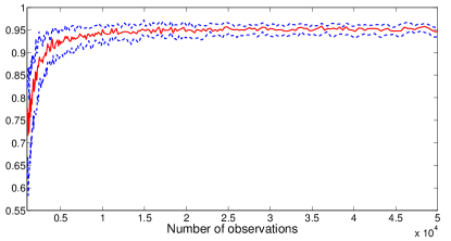
(a) Estimation of $\phi$.

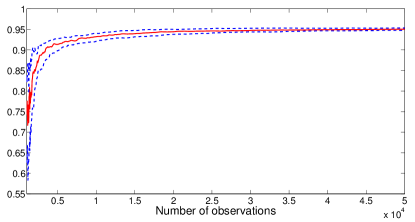
(b) Estimation of $\phi$.

(c) Estimation of $\sigma^{2}$.

(d) Estimation of $\sigma^{2}$.

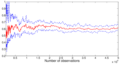
(e) Estimation of $\beta^{2}$.

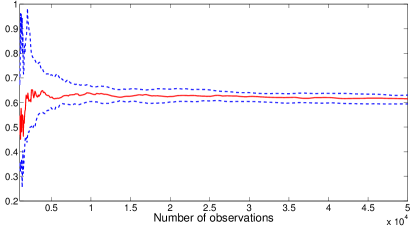
(f) Estimation of $\beta^{2}$.

Figure 1: Estimation of $\phi$, $\sigma^{2}$ and $\beta^{2}$ without (left) and with (right) averaging. Each graph represents the empirical median (bold line) and upper and lower quartiles (dotted line) over $50$ independent Monte Carlo runs. The averaging procedure is started after $1500$ observations. The first $1000$ observations are not displayed for better clarity.

We now discuss the role of the pairs $(\tau_{n},N_{n})$. Roughly speaking (see section 4 for a rigorous decomposition), $\tau$ controls the rate of convergence of $\bar{S}_{\tau}^{T}(\theta,\mathbf{Y})$ to $\lim_{\tau\to\infty}\bar{S}_{\tau}^{T}(\theta,\mathbf{Y})$; and $N$ controls the error between $\bar{S}_{\tau}^{T}(\theta,\mathbf{Y})$ and its SMC approximation. We will show in Section 4 that $\lim_{n}\tau_{n}=\lim_{n}N_{n}=+\infty$ are part of some sufficient conditions for the P-BOEM algorithms to converge. We thus choose increasing sequences $\{\tau_{n},N_{n}\}_{n\geq 1}$. The role of $\tau_{n}$ has been illustrated in [23, Section $3$]. Hence, in this illustration, we fix $\tau_{n}$ and discuss the role of $N_{n}$. Figure 2 compares the algorithms when applied with $\tau_{n}\propto n^{1.1}$ and $N_{n}=\sqrt{\tau_{n}}$ or $N_{n}=\tau_{n}$. The empirical variance (over $50$ independent Monte Carlo runs) of the estimation of $\beta^{2}$ is displayed, as a function of the number of blocks. First, Figure 2 illustrates the variance decrease provided by the averaged procedure, whatever the block size sequence. Moreover, increasing the number of particles per block improves the variance of the estimation given by the P-BOEM algorithm while the impact on the variance of the averaged estimation is less important. On average, the variance is reduced by a factor of $3.0$ for the P-BOEM algorithm and by a factor of $1.8$ for its averaged version when the number of particles goes from $N_{n}=\sqrt{\tau_{n}}$ to $N_{n}=\tau_{n}$. These practical considerations illustrate the theoretical results derived in Section 4.4.

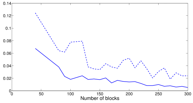
(a) P-BOEM: empirical variance of the estimation of $\beta^{2}$ with $N_{n}=\sqrt{\tau_{n}}$ (dashed line) and $N_{n}=\tau_{n}$ (bold line).

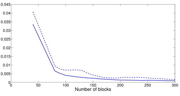
(b) Averaged P-BOEM: empirical variance of the estimation of $\beta^{2}$ with $N_{n}=\sqrt{\tau_{n}}$ (dashed line) and $N_{n}=\tau_{n}$ (bold line).

Figure 2: Empirical variance of the estimation of $\beta^{2}$ with the P-BOEM algorithm (top) and its averaged version (bottom). The averaging procedure is started after the $25$-th block and the variance is displayed after a burn-in time of $35$ blocks.

Finally, we discuss the role of the initial distribution $\chi$. In all the applications above, we have the same distribution $\chi\equiv\mathcal{N}\left(0,(1-\phi^{2})^{-1}\sigma^{2}\right)$ at the beginning of each block. We could choose a different distribution $\chi_{n}$ for each block such as, e.g., the filtering distribution at the end of the previous block. We have observed that this particular choice of $\chi_{n}$ leads to the same behavior for both algorithms.

To end this section, the P-BOEM algorithm is compared to the Online EM algorithm outlined in [4] and [10]. These algorithms rely on a combination of stochastic approximation and SMC methods. According to classical results on stochastic approximation, it is expected that the rate of convergence of the Online EM algorithm behaves like $\gamma_{n}^{1/2}$, where $\{\gamma_{n}\}_{n\geq 0}$ is the so called step-size sequence. Hence, $\gamma_{n}$ in the Online EM algorithm is chosen such that $\gamma_{n}\propto n^{-0.55}$ and the block-size sequence in the P-BOEM algorithm such that $\tau_{n}\propto n^{1.2}$. The number of particles used in the Online EM algorithm is fixed and chosen so that the computational costs of both algorithms are similar. Provided that $N_{n}\propto\tau_{n}$ in the P-BOEM algorithm, this leads to a choice of $70$ particles for the Online EM algorithm. We report in Figure 3, the estimation of $\phi$ and $\sigma^{2}$ for a Polyak-Ruppert averaged Online EM algorithm (see [33]) and the averaged P-BOEM algorithm as a function of the number of observations. The averaging procedure is started after about $1500$ observations. As noted in [23, Section $3$] for a constant sequence $\{N_{n}\}_{n\geq 0}$ this figure shows that both algorithms behave similarly. For the estimation of $\phi$ and $\beta^{2}$, the variance is smaller for the P-BOEM algorithm and the convergence is faster for the P-BOEM algorithm in the case of $\beta^{2}$. Conclusions are different for the estimation of $\sigma^{2}$: the variance is smaller for the P-BOEM algorithm but the Online EM algorithm converges a bit faster. The main advantage of the P-BOEM algorithm is that it relies on approximations which can be controlled in such a way that we are able to show that the limiting points of the P-BOEM algorithms are the stationary points of the limiting normalized log-likelihood of the observations.

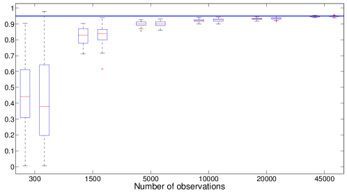
(a) Estimation of $\phi$.

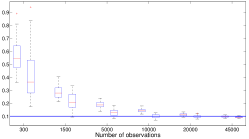
(b) Estimation of $\sigma^{2}$.

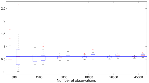
(c) Estimation of $\beta^{2}$.

Figure 3: Estimation of $\phi$, $\sigma^{2}$ and $\beta^{2}$ with the averaged P-BOEM algorithm (left) and a Polyak-Ruppert averaged version of the Online EM algorithm (right) after $300,1500,5000,10000,20000$ and $45000$ observations. The averaging procedure is started after about $1000$ observations (which corresponds to the $25$-th block for the P-BOEM algorithm).

3.2 Simultaneous Localization And Mapping

The Simultaneous Localization And Mapping (SLAM) problem arises when a mobile device wants to build a map of an unknown environment and, at the same time, has to estimate its position in this map. The common statistical approach for the SLAM problem is to introduce a state-space model. Many solutions have been proposed depending on the assumptions made on the transition and observation models, and on the map (see e.g. [2], [28] and [32]). In [28] and [25], it is proposed to see the SLAM as an inference problem in HMM: the localization of the robot is the hidden state with Markovian dynamic, and the map is seen as an unknown parameter. Therefore, the mapping problem is answered by solving the inference task, and the localization problem is answered by approximating the conditional distribution of the hidden states given the observations.

In this application, we consider a statistical model for a landmark-based SLAM problem for a bicycle manoeuvring on a plane surface.

Let $x_{t}\stackrel{{\scriptstyle\mathrm{def}}}{{=}}\{x_{t,i}\}_{i=1}^{3}$ be the robot position, where $x_{t,1}$ and $x_{t,2}$ are the robot’s cartesian coordinates and $x_{t,3}$ its orientation. At each time step, deterministic controls are sent to the robot so that it explores a given part of the environment. Controls are denoted by $(v_{t},\psi_{t})$ where $\psi_{t}$ stands for the robot’s heading direction and $v_{t}$ its velocity. The robot position at time $t$, given its previous position at time $t-1$ and the noisy controls $(\hat{v}_{t},\hat{\psi}_{t})$, can be written as

$$x_{t}=f(x_{t-1},\hat{v}_{t},\hat{\psi}_{t})\;,$$ (14)

where $(\hat{v}_{t},\hat{\psi}_{t})$ is a $2$-dimensional Gaussian distribution with mean $(v_{t},\psi_{t})$ and known covariance matrix $Q$. In this contribution we use the kinematic model of the front wheel of a bicycle (see e.g. [1]) where the function $f$ in (14) is given by

$$f(x_{t-1},\hat{v}_{t},\hat{\psi}_{t})=x_{t-1}+\begin{pmatrix}\hat{v}_{t}d_{t}\cos(x_{t-1,3}+\hat{\psi}_{t})\\ \ \hat{v}_{t}d_{t}\sin(x_{t-1,3}+\hat{\psi}_{t})\\ \hat{v}_{t}d_{t}B^{-1}\sin(\hat{\psi}_{t})\end{pmatrix}\;,$$

where $d_{t}$ is the time period between two successive positions and $B$ is the robot wheelbase.

The $2$-dimensional environment is represented by a set of landmarks $\theta\stackrel{{\scriptstyle\mathrm{def}}}{{=}}\{\theta_{j}\}_{1\leq j\leq q}$, $\theta_{j}\in\mathbb{C}$ being the position of the $j-$th landmark. The total number of landmarks $q$ and the association between observations and landmarks are assumed to be known.

At time $t$, the robot observes the distance and the angular position of all landmarks in its neighborhood; let $c_{t}\subseteq\{1,\cdots,q\}$ be the set of observed landmarks at time $t$. It is assumed that the observations $\{y_{t,i}\}_{i\in c_{t}}$ are independent and satisfy

$$y_{t,i}=h(x_{t},\theta_{i})+\delta_{t,i}\;,$$

where $h$ is defined by

$$h(x,\boldsymbol{\kappa})\stackrel{{\scriptstyle\mathrm{def}}}{{=}}\begin{pmatrix}\sqrt{(\boldsymbol{\kappa}_{1}-x_{1})^{2}+(\boldsymbol{\kappa}_{2}-x_{2})^{2}}\\ \arctan{\frac{\boldsymbol{\kappa}_{2}-x_{2}}{\boldsymbol{\kappa}_{1}-x_{1}}}-x_{3}\end{pmatrix}\;,$$

and the noise vectors $\{\delta_{t,i}\}_{t,i}$ are i.i.d Gaussian $\mathcal{N}\left(0,R\right)$. $R$ is assumed to be known.

The model presented in this Section does not take into account all the issues arising in the SLAM problem (such as the association process which is assumed to be known and the known covariance matrices). The aim is to prove that the BOEM algorithm and its averaged version have satisfying behavior even in the challenging framework described above. The observation and motion models are highly nonlinear and we show that the BOEM algorithm remains stable in this experiment. Several solutions have been proposed to solve the association problem (see e.g. [2] for a solution based on the likelihood of the observations) and could be adapted to our case. We want to estimate $\theta=\{\theta_{j}\}_{j=1}^{q}$ by applying the P-BOEM algorithms. In this paper, we use simulated data. $q=15$ landmarks are drawn in a square of size $45m\mathrm{x}45m$. The robot path is sampled with a given set of controls. Using the true positions of all landmarks in the map and the true path of the robot (see the dots and the bold line on Figure 4), observations are sampled by setting: $R=\begin{pmatrix}\sigma_{r}^{2}&\rho\\ \rho&\sigma_{b}^{2}\end{pmatrix}\;,$ where $\sigma_{r}=0.5\mbox{m}$, $\sigma_{b}=\frac{\pi}{60}\mbox{rad}$ and $\rho=0.01$. We choose $Q=\mbox{diag}(\sigma_{v}^{2},\sigma_{\phi}^{2})$ where $\sigma_{v}=0.5\mbox{m.s}^{-1}$, $\sigma_{\psi}=\frac{\pi}{60}\mbox{rad}$ and $B=1.5\mathrm{m}$.

In this model, the transition denoted by $m_{\theta}$ does not depend on the map $\theta$ (see (14)) and the marginal likelihood $g_{\theta}$ is such that the complete data likelihood does not belong to the curved exponential family:

$$\sum_{i\in c_{t}}\ln g_{\theta}(x_{t},y_{t,i})\propto\sum_{i\in c_{t}}\left[y_{t,i}-h(x_{t},\theta_{i})\right]^{\star}R^{-1}\left[y_{t,i}-h(x_{t},\theta_{i})\right]\;.$$ (15)

Hence, in order to apply Algorithm 1, at the beginning of each block, $g_{\theta}$ is approximated by a function depending on the current parameter estimate so that the resulting approximated model belongs to the curved exponential family (see [25]). As can be seen from (15), approximating the function $\boldsymbol{\kappa}\mapsto h(x,\boldsymbol{\kappa})$ by its first-order Taylor expansion at $\theta_{i}$ leads to a quadratic approximation of $g_{\theta}$. This approach is commonly used in the SLAM framework to use the properties of linear Gaussian models (see e.g. [2]).

As the landmarks are not observed all the time, we choose a slowly increasing sequence $\{\tau_{n}\propto n^{1.1}\}_{n\geq 1}$ so that the number of updates is not too small (in this experiment, we have $60$ updates for a total number of observations of $2000$). As the total number of observations is not so large (the largest block is of length $60$), the number of particles is chosen to be constant on each block: for all $n\geq 1$, $N_{n}=50$. For the SMC step, we apply Algorithm 2 with the bootstrap filter.

For each run the estimated path (equal to the weighted mean of the particles) and the estimated map at the end of the loop ($T=2000$) are stored. Figure 4 represents the mean estimated path and the mean map over $50$ independent Monte Carlo runs. It highlights the good performance of the P-BOEM algorithm in a more complex framework.

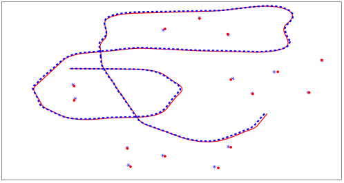
Figure 4: True trajectory (bold line) and true landmark positions (balls) with the estimated path (dotted line) and the landmarks’ estimated positions (stars) at the end of the run ($T=2000$).

We also compare our algorithm to the marginal SLAM algorithm proposed by [28]. In this algorithm, the map is also modeled as a parameter to learn in a HMM model; SMC methods are used to estimate the map in the maximum likelihood sense. The Marginal SLAM algorithm is a gradient-based approach for solving the recursive maximum likelihood procedure. Note that, in the case of i.i.d. observations, [35] proposed to update the parameter estimate each time a new observation is available using a stochastic gradient approach. Figure 5 illustrates the estimation of the position of each landmark. The P-BOEM algorithm is applied using the same parameters as above and the marginal SLAM algorithm uses a sequence of step-size $\{\gamma_{n}\propto n^{-0.6}\}_{n\geq 1}$. We use the averaged version of the P-BOEM algorithm and a Polyak-Ruppert based averaging procedure for the marginal SLAM algorithm (see [33]). For each landmark the last estimation (at the end of the loop) of the position is stored for each of the $50$ independent Monte Carlo runs. Figure 5 displays the distance between the estimated position and the true position for each landmark. In this experiment, the P-BOEM based SLAM algorithm outperforms the marginal SLAM algorithm.

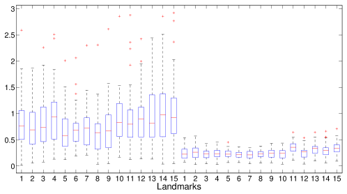
Figure 5: Distance between the final estimation and the true position for each of the $15$ landmarks with the averaged marginal SLAM algorithm (left) and the averaged P-BOEM algorithm (right).

4 Convergence of the Particle Block Online EM algorithms

In this section, we analyze the limiting points of the P-BOEM algorithm. We prove in Theorem 4.3 that the P-BOEM algorithm has the same limit points as a so-called limiting EM algorithm, which defines a sequence $\{\theta_{n}\}_{n\geq 0}$ by $\theta_{n+1}=\bar{\theta}\left[\bar{S}(\theta_{n})\right]$ where $\bar{S}(\theta)$ is the a.s. limit $\lim_{\tau\to+\infty}\bar{S}_{\tau}^{T}(\theta,\mathbf{Y})$ (defined by (6)). As discussed in [23, Section 4.3.], the set of limit points of the limiting EM algorithm is the set of stationary points of the contrast function $\ell(\theta)$, defined as the a.s. limit of the normalized log-likelihood of the observations, when $T\to+\infty$. The convergence result below on the P-BOEM algorithm requires two sets of assumptions: conditions AA2 to AA5 are the same as in [23] and imply the convergence of the BOEM algorithm; assumptions AA6 and AA7 are introduced to control the Monte Carlo error.

4.1 Assumptions

Consider the following assumptions

• There exist $\sigma_{-}$ and $\sigma_{+}$ s.t. for any $\left(x,x^{\prime}\right)\in\mathbb{X}^{2}$ and any $\theta\in\Theta$, $0<\sigma_{-}\leq m_{\theta}(x,x^{\prime})\leq\sigma_{+}$. Set $\rho\stackrel{{\scriptstyle\mathrm{def}}}{{=}}1-(\sigma_{-}/\sigma_{+})\;.$

Define, for all $y\in\mathbb{Y}$,

$$b_{-}(y)\stackrel{{\scriptstyle\mathrm{def}}}{{=}}\inf_{\theta\in\Theta}\int g_{\theta}(x,y)\lambda(\mathrm{d}x)\quad\mbox{and}\quad b_{+}(y)\stackrel{{\scriptstyle\mathrm{def}}}{{=}}\sup_{\theta\in\Theta}\int g_{\theta}(x,y)\lambda(\mathrm{d}x)\;.$$ (16)

For any sequence of r.v. $Z\stackrel{{\scriptstyle\mathrm{def}}}{{=}}\{Z_{t}\}_{t\in\mathbb{Z}}$ on $(\Omega,\widetilde{\mathbb{P}},\mathcal{F})$, let

$$\mathcal{F}_{k}^{Z}\stackrel{{\scriptstyle\mathrm{def}}}{{=}}\sigma\left(\{Z_{u}\}_{u\leq k}\right)\quad\mbox{and}\quad\mathcal{G}_{k}^{Z}\stackrel{{\scriptstyle\mathrm{def}}}{{=}}\sigma\left(\{Z_{u}\}_{u\geq k}\right)$$ (17)

be $\sigma$-fields associated to $Z$. We also define the mixing coefficients by, see [7],

$$\beta^{Z}(n)\stackrel{{\scriptstyle\mathrm{def}}}{{=}}\underset{u\in\mathbb{Z}}{\sup}\,\beta(\mathcal{G}_{u+n}^{Z},\mathcal{F}_{u}^{Z})\;,\forall\;n\geq 0\;,$$ (18)

where for any $\sigma$-algebras $\mathcal{F}$ and $\mathcal{G}$,

$$\beta(\mathcal{G},\mathcal{F})\stackrel{{\scriptstyle\mathrm{def}}}{{=}}\underset{B\in\mathcal{G}}{\sup}\,|\widetilde{\mathbb{P}}(B|\mathcal{F})-\widetilde{\mathbb{P}}(B)|\;.$$ (19)

For $p>0$ and $Z$ a $\mathbb{R}^{d}$-valued random variable measurable w.r.t. the $\sigma$-algebra $\mathcal{F}$, set

$$\left\|Z\right\|_{p}\stackrel{{\scriptstyle\mathrm{def}}}{{=}}\left(\mathbb{E}\left[|Z|^{p}\right]\right)^{1/p}\;.$$

• -($p$) $\left\|\sup_{x,x^{\prime}\in\mathbb{X}^{2}}\,|S(x,x^{\prime},\mathbf{Y}_{0})|\right\|_{p}<+\infty\;.$

• 1. $\mathbf{Y}$ is a stationary sequence such that there exist $C\in[0,1)$ and $\beta\in(0,1)$ satisfying, for any $n\geq 0$, $\beta^{\mathbf{Y}}(n)\leq C\beta^{n}$, where $\beta^{\mathbf{Y}}$ is defined in (18).

  2. $\mathbb{E}\left[|\log b_{-}(\mathbf{Y}_{0})|+|\log b_{+}(\mathbf{Y}_{0})|\right]<+\infty$.

• There exist $c>0$ and $a>1$ such that for all $n\geq 1$, $\tau_{n}=\lfloor cn^{a}\rfloor$.

Assumptions AA2 to AA5 are the same as in [23]. AA2, referred to as the strong mixing condition, is used to prove the uniform forgetting property of the initial condition of the filter, see e.g. [11] and [12]. This assumption is easy to check in finite state-space HMM or when the state-space is compact when the Markov kernel $\boldsymbol{m_{\theta}}$ is sufficiently regular. As noted in [23], it can fail to hold in quite general situations. Nevertheless, the exponential forgetting property needed to ensure the convergence results could be checked under weaker assumptions (see [15] for a Doeblin assumption). However, it would imply quite technical supplementary results out of the scope of this paper. Examples of observation sequences satisfying AA4 include, for example, stationary $\psi$-irreducible and positive recurrent Markov chains which are geometrically ergodic (see e.g. [31] for Markov chains theory).

We need to control the $\mathrm{L}_{p}$-mean error on each block between $\bar{S}_{\tau_{n+1}}^{T_{n}}(\theta_{n},\mathbf{Y})$ and its SMC approximation. This control is discussed in Section 4.2 below when the SMC approximation is computed as described in Section 2.4.

4.2 $\mathrm{L}_{p}$-error of the SMC approximation

For each block $n$, denote by $\{\upsilon_{t,n}\}_{t\leq\tau_{n+1}}$ and $\{q_{t,n}\}_{t\leq\tau_{n+1}}$ respectively the adjustment multipliers and the instrumental kernels in the SMC propagation step (see (13)). For all $y\in\mathbb{Y}$, define

$$\omega_{+}(y)=\underset{\theta\in\Theta}{\sup}\,\underset{\begin{subarray}{c}(x,x^{{}^{\prime}})\in\mathbb{X}\times\mathbb{X}\\ t\geq 0,n\geq 0\end{subarray}}{\sup}\dfrac{m_{\theta}(x,x^{\prime})g_{\theta}(x^{\prime},y)}{\upsilon_{t,n}(x)q_{t,n}(x,x^{\prime})}\;.$$

Consider the following assumptions.

• $|\upsilon|_{\infty}\stackrel{{\scriptstyle\mathrm{def}}}{{=}}\sup_{t,n}|\upsilon_{t,n}|_{\infty}<\infty$.

• -($p$) $\left\|\frac{\omega_{+}(\mathbf{Y}_{0})}{b_{-}(\mathbf{Y}_{0})}\right\|_{p}<+\infty\;.$

In the case of the Bootstrap filter, AA6 holds (since $v_{t,n}=1$) and $\omega_{+}(y)=\underset{\theta\in\Theta}{\sup}\,\underset{\begin{subarray}{c}x\in\mathbb{X}\end{subarray}}{\sup}\,g_{\theta}(x,y)$.

Proposition 4.1.

Let $S:\mathbb{X}^{2}\times\mathbb{Y}\longrightarrow\mathbb{R}^{d}$ be a measurable function s.t. AA3-($\bar{p}$) holds for some $\bar{p}>2$. Assume AA2, AA4, AA6. Define $\Delta p\stackrel{{\scriptstyle\mathrm{def}}}{{=}}2\bar{p}p/(\bar{p}-p)$ and assume AA7-($\Delta p$) holds for some $p\in(2,\bar{p})$. Then, there exists a constant $C$ s.t. for all $n\geq 0$,

$$\left\|\widetilde{S}_{n}(\theta_{n},\mathbf{Y})-\bar{S}_{\tau_{n+1}}^{T_{n}}(\theta_{n},\mathbf{Y})\right\|_{p}\leq C\left(\frac{1}{N_{n+1}}+\frac{1}{\tau_{n+1}^{1/2}N_{n+1}^{1/2}}\right)\;,$$

where $\widetilde{S}_{n}(\theta_{n},\mathbf{Y})$ is computed with the algorithm described in Section 2.4.

4.3 Asymptotic behavior of the Particle Block Online EM algorithms

Following [23], we address the convergence of the P-BOEM algorithm as the convergence of a perturbed version of the limiting EM recursion. The following result, which is proved in [23, Theorem 4.1.], shows that when $\tau$ is large, the BOEM statistic $\bar{S}^{T}_{\tau}(\theta,\mathbf{Y})$ is an approximation of a deterministic quantity $\bar{\mathrm{S}}(\theta)$; the limiting EM algorithm is the iterative procedure defined by $\theta_{n+1}=\mathrm{R}(\theta_{n})$ where

$$\mathrm{R}(\theta)\stackrel{{\scriptstyle\mathrm{def}}}{{=}}\bar{\theta}(\bar{\mathrm{S}}(\theta))\;,\forall\theta\in\Theta\;;$$ (20)

the mapping $\bar{\theta}$ is given by AA1.

Theorem 4.2.

Let $S:\mathbb{X}^{2}\times\mathbb{Y}\longrightarrow\mathbb{R}^{d}$ be a measurable function s.t. AA3-($1$) holds. Assume AA2 and AA4(a). For any $\theta\in\Theta$, there exists a $\mathbb{P}$-integrable r.v. $\mathbb{E}_{\theta}\left[S(X_{-1},X_{0},\mathbf{Y}_{0})\middle|\mathbf{Y}\right]$ s.t. for any $T>0$,

$$\bar{S}_{\tau}^{T}(\theta,\mathbf{Y})\underset{\tau\rightarrow+\infty}{\longrightarrow}\bar{\mathrm{S}}(\theta)\stackrel{{\scriptstyle\mathrm{def}}}{{=}}\mathbb{E}\left[\mathbb{E}_{\theta}\left[S(X_{-1},X_{0},\mathbf{Y}_{0})\middle|\mathbf{Y}\right]\right]\;,\quad\mathbb{P}-\mathrm{a.s.}$$ (21)

Moreover, $\theta\mapsto\bar{\mathrm{S}}(\theta)$ is continuous on $\Theta$.

The asymptotic behavior of the limiting EM algorithm is addressed in [23, Section $4.2$]: the main ingredient is that the map $\mathrm{R}$ admits a positive and continuous Lyapunov function $\mathrm{W}$ w.r.t. the set

$$\mathcal{L}\stackrel{{\scriptstyle\mathrm{def}}}{{=}}\{\theta\in\Theta;\mathrm{R}(\theta)=\theta\}\;,$$ (22)

i.e. (i) $\mathrm{W}\circ\mathrm{R}(\theta)\geq\mathrm{W}(\theta)$ for any $\theta\in\Theta$ and, (ii) for any compact subset $\mathcal{K}$ of $\Theta\setminus\mathcal{L}$, $\inf_{\theta\in\mathcal{K}}\mathrm{W}\circ\mathrm{R}(\theta)-\mathrm{W}(\theta)>0$. This Lyapunov function is equal to $\exp(\ell(\theta))$, where the contrast function $\ell(\theta)$ is the (deterministic) limit of the normalized log-likelihood of the observations when $T\to+\infty$ (see [24, Theorem $4.9$]).

Theorem 4.3 establishes the convergence of the P-BOEM algorithm to the set $\mathcal{L}$ defined by (22). The proof of Theorem 4.3 is an application of [23, Theorem $4.4$]. An additional assumption on the number of particles per block is required to check [23, A$6$] (note indeed that AA8 below and Proposition 4.1 imply the condition in [23] about the $\mathrm{L}_{p}$-control of the error).

• There exist $c>0$ and $d\geq(a+1)/2a$ (where $a$ is given by AA5) such that, for all $n\geq 1$, $N_{n}=\lfloor c\tau_{n}^{d}\rfloor$.

Theorem 4.3.

Assume AA1-A2, AA3-($\bar{p}$), AA4-A6 and AA8 for some $\bar{p}>2$. Define $\Delta p\stackrel{{\scriptstyle\mathrm{def}}}{{=}}2\bar{p}p/(\bar{p}-p)$ and assume AA7-($\Delta p$) holds for some $p\in(2,\bar{p})$. Assume in addition that $\mathrm{W}(\mathcal{L})$ has an empty interior. Then, there exists $w_{\star}$ s.t. $\{\mathrm{W}(\theta_{n})\}_{n\geq 0}$ converges almost surely to $w_{\star}$ and $\{\theta_{n}\}_{n\geq 0}$ converges to $\{\theta\in\mathcal{L};\mathrm{W}(\theta)=w_{\star}\}$.

The assumption on $\mathrm{W}(\mathcal{L})$ made in Theorem 4.3 is in common use to prove the convergence of EM based procedures or stochastic approximation algorithms. It is used in [36] to find the limit points of the classical EM algorithm. See also [13] and [20] for the stability of the Monte Carlo EM algorithm and of a stochastic approximation of the EM algorithm. If $\mathrm{W}$ is sufficiently regular, Sard’s theorem states that $\mathrm{W}(\mathcal{L})$ has Lebesgue measure $0$ and hence has an empty interior.

Under the assumptions of Theorem 4.3, it can be proved that, along any converging P-BOEM sequence $\{\theta_{n}\}_{n\geq 0}$ to $\theta_{\star}$ in $\mathcal{L}$, the averaged P-BOEM statistics $\{\widetilde{\Sigma}_{n}\}_{n}$ defined by (7) (see also (9)) converge to $\bar{\mathrm{S}}(\theta_{\star})$, see Proposition 5.2. Since $\bar{\theta}$ is continuous, the averaged P-BOEM sequence $\{\widetilde{\theta}_{n}\}_{n\geq 0}$ converges to $\bar{\theta}(\bar{\mathrm{S}}(\theta_{\star}))=\mathrm{R}(\theta_{\star})$. Since $\theta_{\star}\in\mathcal{L}$, $\mathrm{R}(\theta_{\star})=\theta_{\star}$, showing that the averaged P-BOEM algorithm has the same limit points as the P-BOEM algorithm.

4.4 Rate of convergence of the Particle Block Online EM algorithms

In this section, we consider a converging P-BOEM sequence $\{\theta_{n}\}_{n\geq 0}$ with limiting point $\theta_{\star}\in\mathcal{L}$. It can be shown, as in [24, Proposition $3.1$], that the convergence of the sequence $\{\theta_{n}\}_{n\geq 0}$ is equivalent to the convergence of the sufficient statistics $\{\widetilde{S}_{n}(\theta_{n},\mathbf{Y})\}_{n\geq 0}$: along any P-BOEM sequence converging to $\theta_{\star}$, this sequence of sufficient statistics converges to $s_{\star}=\bar{\mathrm{S}}(\theta_{\star})$. Let $\mathrm{G}:\mathcal{S}\to\mathcal{S}$ be the limiting EM map defined on the space of sufficient statistics by

$$\mathrm{G}(s)\stackrel{{\scriptstyle\mathrm{def}}}{{=}}\bar{\mathrm{S}}(\bar{\theta}(s))\;,\qquad\forall s\in\mathcal{S}\;.$$ (23)

To that goal consider the following assumption.

• 1. $\bar{\mathrm{S}}$ and $\bar{\theta}$ are twice continuously differentiable on $\Theta$ and $\mathcal{S}$.

  2. $\mathrm{sp}(\nabla_{s}\mathrm{G}(s_{\star}))\in(0,1)$ where $\mathrm{sp}$ denotes the spectral radius.

We will use the following notation: for any sequence of random variables $\{Z_{n}\}_{n\geq 0}$, write $Z_{n}=O_{\mathrm{L}_{p}}(1)$ if $\limsup_{n}\left\|Z_{n}\right\|_{p}<\infty$; and $Z_{n}=O_{\mathrm{a.s}}(1)$ if $\sup_{n}|Z_{n}|<+\infty$ $\mathbb{P}-\mathrm{a.s.}$

Theorem 4.4.

Assume AA1-A2, AA3-($\bar{p}$), AA4-A6 and AA8-A9 for some $\bar{p}>2$. Define $\Delta p\stackrel{{\scriptstyle\mathrm{def}}}{{=}}2\bar{p}p/(\bar{p}-p)$ and assume AA7-($\Delta p$) holds for some $p\in(2,\bar{p})$. Then,

$$\left[\theta_{n}-\theta_{\star}\right]\mathbf{1}_{\lim_{k}\theta_{k}=\theta_{\star}}=O_{\mathrm{L}_{p/2}}\left(\frac{1}{\tau_{n}^{1/2}}\right)O_{\mathrm{a.s}}\left(1\right)\;.$$ (24)

On the other hand, for the averaged sequence,

$$\left[\widetilde{\theta}_{n}-\theta_{\star}\right]\mathbf{1}_{\lim_{k}\theta_{k}=\theta_{\star}}=O_{\mathrm{L}_{p/2}}\left(\frac{1}{T_{n}^{1/2}}\right)O_{\mathrm{a.s}}\left(1\right)\;.$$ (25)

The proof of Theorem 4.4 is obtained by checking the assumptions of [23, Theorem $5.1$ and Theorem $5.2$].

Eq. (24) shows that the error $\theta_{n}-\theta_{\star}$ has a $\mathrm{L}_{p/2}$-norm decreasing as $\tau_{n}^{-1/2}$. This result is obtained by assuming $N_{n}\sim\tau_{n}^{d}$, with $d\geq(a+1)/2a$, which implies that the SMC error and the BOEM error are balanced. Unfortunately, such a rate is obtained after a total number of observations $T_{n}$; therefore, as discussed in [23], it is quite sub-optimal. Eq (25) shows that the rate of convergence equal to the square root of the total number of observations up to block $n$, can be reached by using the averaged P-BOEM algorithm: the $\mathrm{L}_{p/2}$-norm of the error $\widetilde{\theta}_{n}-\theta_{\star}$ has a rate of convergence proportional to $T_{n}^{-1/2}$. Here again, note that since $N_{n}$ is chosen as in AA8 the SMC error and the BOEM error are balanced.

5 Proofs

For a function $h$, define $\mathrm{osc}(h)\stackrel{{\scriptstyle\mathrm{def}}}{{=}}\sup_{z,z^{\prime}}|h(z)-h(z^{\prime})|$.

5.1 Proof of Proposition 4.1

For any $t\in\{0,\dots,\tau_{n+1}\}$, define the $\sigma$-algebra $\mathcal{F}_{n,t}^{N_{n+1}}$ by

$$\mathcal{F}_{n,t}^{N_{n+1}}\stackrel{{\scriptstyle\mathrm{def}}}{{=}}\sigma\left\{\theta_{n},\mathbf{Y}_{T_{n}+1:T_{n}+t+1},\left(\xi_{s}^{\ell},\omega_{s}^{\ell}\right);\ell\in\{1,\dots,N_{n+1}\};0\leq s\leq t\right\}\;.$$ (26)

We use $S_{s}(x,x^{\prime})$ as a shorthand notation for $S(x,x^{\prime},\mathbf{Y}_{s})$. Under AA2 and AA6, Propositions B.$5$.,  B.$8$. and B.$9$. in Appendix B of [22] can be applied so that

$$\mathbb{E}\left[\left|\widetilde{S}_{n}(\theta_{n},\mathbf{Y})-\bar{S}_{\tau_{n+1}}^{T_{n}}(\theta_{n},\mathbf{Y})\right|^{p}\right]\leq C\left(I_{1,n}+I_{2,n}\right)\;,$$ (27)

where

$$I_{1,n} \stackrel{{\scriptstyle\mathrm{def}}}{{=}}\frac{1}{\tau_{n+1}^{\frac{p}{2}+1}N_{n+1}^{\frac{p}{2}}}\times\sum_{t=0}^{\tau_{n+1}}\mathbb{E}\left[\left|\frac{\omega_{+}(\mathbf{Y}_{t+T_{n}})}{b_{-}(\mathbf{Y}_{t+T_{n}})}\sum_{s=1}^{\tau_{n+1}}\rho^{|t-s|}\mathrm{osc}\{S_{s+T_{n}}\}\right|^{p}\right]\;,$$

$$I_{2,n} \stackrel{{\scriptstyle\mathrm{def}}}{{=}}\frac{1}{\tau_{n+1}N_{n+1}^{p}}\,$$

$$\hskip 25.6073pt\times\sum_{t=0}^{\tau_{n+1}}\mathbb{E}\left[\left|\frac{\omega_{+}(\mathbf{Y}_{t+T_{n}})}{b_{-}(\mathbf{Y}_{t+T_{n}})}\right|^{2p}\mathbb{E}\left[\left|\sum_{s=1}^{\tau_{n+1}}\rho^{|t-s|}\mathrm{osc}\{S_{s+T_{n}}\}\right|^{\bar{p}}\middle|\mathcal{F}_{n,t-1}^{N_{n+1}}\right]^{p/\bar{p}}\right]\;.$$

By the Hölder inequality applied with $\alpha\stackrel{{\scriptstyle\mathrm{def}}}{{=}}\bar{p}/p\geq 1$ and $\beta^{-1}\stackrel{{\scriptstyle\mathrm{def}}}{{=}}1-\alpha^{-1}$,

$$I_{1,n}\leq\frac{1}{\tau_{n+1}^{\frac{p}{2}+1}N_{n+1}^{\frac{p}{2}}}\sum_{t=1}^{\tau_{n+1}}\left\|\sum_{s=1}^{\tau_{n+1}}\rho^{|t-s|}\mathrm{osc}\{S_{s+T_{n}}\}\right\|_{\bar{p}}^{p}\times\left\|\frac{\omega_{+}(\mathbf{Y}_{t+T_{n}})}{b_{-}(\mathbf{Y}_{t+T_{n}})}\right\|_{2\bar{p}p/(\bar{p}-p)}^{2p}\;.$$

By AA2, AA3-($\bar{p}$), AA4(a) and AA7-($\Delta p$), we have

$$I_{1,n}\leq\frac{C}{\tau_{n+1}^{\frac{p}{2}}N_{n+1}^{\frac{p}{2}}}\;.$$

Using similar arguments for $I_{2,n}$ yields $I_{2,n}\leq C\,N_{n+1}^{-p}$, which concludes the proof.

5.2 $\mathrm{L}_{p}$-controls

Proposition 5.1.

Let $S:\mathbb{X}^{2}\times\mathbb{Y}\longrightarrow\mathbb{R}^{d}$ be a measurable function s.t. AA3-($\bar{p}$) holds for some $\bar{p}>2$. Assume AA2, AA4, AA6 and AA7-($\Delta p$) for some $p\in(2,\bar{p})$, where $\Delta p\stackrel{{\scriptstyle\mathrm{def}}}{{=}}2\bar{p}p/(\bar{p}-p)$. There exists a constant $C$ s.t. for any $n\geq 1$,

$$\left\|\widetilde{S}_{n}(\theta_{n},\mathbf{Y})-\bar{\mathrm{S}}(\theta_{n})\right\|_{p}{}\leq C\left(\frac{1}{\sqrt{\tau_{n+1}}}+\frac{1}{N_{n+1}}\right)\;.$$

Proof.

Under AA2, AA3-($\bar{p}$) and AA4, by [23, Theorem $4.1$], there exists a constant $C$ s.t.

$$\left\|\bar{S}_{\tau_{n+1}}^{T_{n}}(\theta_{n},\mathbf{Y})-\bar{\mathrm{S}}(\theta_{n})\right\|_{p}\leq\frac{C}{\sqrt{\tau_{n+1}}}\;.$$

Moreover, under AA6 and AA7-($\Delta p$), by Proposition 4.1, we have

$$\left\|\widetilde{S}_{n}(\theta_{n},\mathbf{Y})-\bar{S}_{\tau_{n+1}}^{T_{n}}(\theta_{n},\mathbf{Y})\right\|_{p}\leq C\left(\frac{1}{N_{n+1}}+\frac{1}{\tau^{1/2}_{n+1}N_{n+1}^{1/2}}\right)\;,$$

which concludes the proof. ∎

Proposition 5.2.

Let $S:\mathbb{X}^{2}\times\mathbb{Y}\longrightarrow\mathbb{R}^{d}$ be a measurable function s.t. AA3-($\bar{p}$) holds for some $\bar{p}>2$. Assume AA2, AA4-A5, AA6-A8 and AA7-($\Delta p$) for some $p\in(2,\bar{p})$, where $\Delta p\stackrel{{\scriptstyle\mathrm{def}}}{{=}}2\bar{p}p/(\bar{p}-p)$. Let $\{\theta_{n}\}_{n}$ be the P-BOEM sequence. For any $\theta_{\star}\in\Theta$, on the set $\{\lim_{n}\theta_{n}=\theta_{\star}\}$,

$$\widetilde{\Sigma}_{n}\longrightarrow\bar{\mathrm{S}}(\theta_{\star})\;,\quad\mathbb{P}-\mathrm{a.s.}\;,$$

where $\bar{\mathrm{S}}$ is defined in (21) and $\widetilde{\Sigma}_{n}$ in (7).

Proof.

By (7), $\widetilde{\Sigma}_{n}$ can be written as

$$\widetilde{\Sigma}_{n}=\frac{1}{T_{n}}\sum_{j=1}^{n}\tau_{j}\,\left[\widetilde{S}_{j-1}(\theta_{j-1},\mathbf{Y})-\bar{\mathrm{S}}(\theta_{j-1})\right]+\frac{1}{T_{n}}\sum_{j=1}^{n}\tau_{j}\,\bar{\mathrm{S}}(\theta_{j-1})\;.$$ (28)

By Theorem 4.2, $\bar{\mathrm{S}}$ is continuous so, by the Cesaro Lemma, the second term in the right-hand side of (28) converges to $\bar{\mathrm{S}}(\theta_{\star})$ $\mathbb{P}$-a.s., on the set $\{\lim_{n}\theta_{n}=\theta_{\star}\}$. By Proposition 5.1, there exists a constant $C$ such that for any $n$,

$$\left\|\widetilde{S}_{n}(\theta_{n},\mathbf{Y})-\bar{\mathrm{S}}(\theta_{n})\right\|_{p}\leq C\left(\frac{1}{\sqrt{\tau_{n+1}}}+\frac{1}{N_{n+1}}\right)\;.$$

Hence, by AA5, AA8 and the Borel-Cantelli Lemma,

$$\left|\widetilde{S}_{n}(\theta_{n},\mathbf{Y})-\bar{\mathrm{S}}(\theta_{n})\right|\longrightarrow 0\;,\quad\mathbb{P}-\mathrm{a.s.}$$

The proof is concluded by applying the Cesaro Lemma. ∎

Appendix A Detailed SMC algorithm

In this section, we give a detailed description of the SMC algorithm used to compute sequentially the quantities $\widetilde{S}_{n}(\theta_{n},\mathbf{Y})$, $n\geq 0$. This is the algorithm proposed by  [4] and [10].

At each time step, the weighted samples are produced using sequential importance sampling and sampling importance resampling steps. In Algorithm 2, the instrumental proposition kernel used to select and propagate the particles is $\pi_{t}$ (see (13) and [16, 17, 27] for further details on this SMC step).

It is readily seen from the description below that the observations $\mathbf{Y}_{t}$ are processed sequentially.

Algorithm 2 Forward SMC step

0:  $\theta_{n}$, $\tau_{n+1}$, $N$, $\mathbf{Y}_{T_{n}+1:T_{n}+\tau_{n+1}}\;.$

0:  $\widetilde{S}_{n}(\theta_{n},\mathbf{Y})\;.$

  Sample $\{\xi_{0}^{\ell}\}_{\ell=1}^{N}$ i.i.d. with distribution $\chi\;.$

  Set $\omega_{0}^{\ell}=1/N$ for all $\ell\in\{1,\dots,N\}\;.$

  Set $R_{0,\theta_{n}}^{\ell}=0$ for all $\ell\in\{1,\dots,N\}\;.$

  for $t=1$ to $\tau_{n+1}$ do

     for $\ell=1$ to $N$ do

        Conditionally to $(\theta_{n},Y_{T_{n}+1:T_{n}+t},\{J_{t-1}^{\ell},\xi_{t-1}^{\ell}\}_{\ell=1}^{N})$, sample independently $(J_{t}^{\ell},\xi_{t}^{\ell})\sim\pi_{t}(i,\mathrm{d}x)\;,$ where $\pi_{t}(i,\mathrm{d}x)\propto\omega_{t-1}^{i}\upsilon_{t}(\xi_{t-1}^{i})q_{t}(\xi_{t-1}^{i},x)\lambda(\mathrm{d}x)\;.$

        Set

$$\omega_{t}^{\ell}=\frac{m_{\theta_{n}}(\xi_{t-1}^{J_{t}^{\ell}},\xi_{t}^{\ell})g_{\theta_{n}}(\xi_{t}^{\ell},\mathbf{Y}_{T_{n}+t})}{\upsilon_{t}(\xi_{t-1}^{J_{t}^{\ell}})q_{t}(\xi_{t-1}^{J_{t}^{\ell}},\xi_{t}^{\ell})}\;.$$

        Set

$$R_{t,\theta_{n}}^{\ell}=\frac{1}{t}\sum_{j=1}^{N}\omega_{t-1}^{j}m_{\theta_{n}}(\xi_{t-1}^{j},\xi_{t}^{\ell})\frac{S(\xi_{t-1}^{j},\xi_{t}^{\ell},\mathbf{Y}_{T_{n}+t})+(t-1)R_{t-1,\theta_{n}}^{j}}{\sum_{k=1}^{N}\omega_{t-1}^{k}m_{\theta_{n}}(\xi_{t-1}^{k},\xi_{t}^{\ell})}\;.$$

     end for

  end for

  Set

$$\widetilde{S}_{n}(\theta_{n},\mathbf{Y})=\sum_{\ell=1}^{N}\omega_{\tau_{n+1}}^{\ell}R_{\tau_{n+1},\theta_{n}}^{\ell}\;.$$

Appendix B $\mathrm{L}_{p}$-controls of SMC approximations

In this section, we give further details on the $\mathrm{L}_{p}$ control on each block (see  (27)):

$$\mathbb{E}\left[\left|\widetilde{S}_{\tau_{n+1}}^{N,T_{n}}(\theta_{n},\mathbf{Y})-\bar{S}_{\tau_{n+1}}^{T_{n}}(\theta_{n},\mathbf{Y})\right|^{p}\right]\;,$$

$\bar{S}_{\tau}^{T}$ is defined by (6) (we recall that, $\chi$ being fixed, it is dropped from the notations) and $\widetilde{S}_{\tau}^{N,T}$ is the SMC approximation of $\bar{S}_{\tau}^{T}$ based on $N$ particles computed as described in Section 2.4.

The following results are technical lemmas taken from [16] (stated here for a better clarity) or extensions of the $\mathrm{L}_{p}$ controls derived in [19].

Hereafter, “time $t$” corresponds to time $t$ in the block $n$. Therefore, even if it is not explicit in the notations (in order to make them simpler), the following quantities depend upon the observations $\mathbf{Y}_{T_{n}+1:T_{n}+\tau_{n+1}}$.

Denote by $\phi_{s}^{\theta}$ the filtering distribution at time $s$, and let

$$\mathrm{B}_{\phi_{t}^{\theta}}^{\theta}(x,\mathrm{d}x^{\prime})\stackrel{{\scriptstyle\mathrm{def}}}{{=}}\frac{m_{\theta}(x^{\prime},x)}{\int m_{\theta}(u,x)\phi_{t}^{\theta}(\mathrm{d}u)}\phi_{t}^{\theta}(\mathrm{d}x^{\prime})$$

be the backward kernel smoothing kernel at time $t+1$. For all $0\leq s\leq\tau-1$ and for all bounded measurable function $h$ on $\mathbb{X}^{\tau-s+1}$, define recursively $\phi_{s:\tau|\tau}^{\theta}[h]$ backward in time, according to

$$\phi_{s:\tau|\tau}^{\theta}[h]=\idotsint\mathrm{B}_{\phi_{s}^{\theta}}^{\theta}(x_{s+1},\mathrm{d}x_{s})\,\phi_{s+1:\tau|\tau}^{\theta}(\mathrm{d}{x}_{s+1:\tau})\,h({x}_{s:\tau})\;,$$ (29)

starting from $\phi_{\tau:\tau|\tau}^{\theta}=\phi_{\tau}^{\theta}$. By convention, $\phi_{0}^{\theta}=\chi$.

For $t\geq 1$, let $\left\{(\xi_{t}^{\ell},\omega_{t}^{\ell})\right\}_{\ell=1}^{N}$ be the weighted samples obtained as described in Section 2.4 (see also Algorithm 2 in Appendix A); it approximates the filtering distribution $\phi_{t}^{\theta}$. Denote by $\phi_{t}^{N,\theta}$ this approximation. For $0\leq s\leq\tau-1$, an approximation of the backward kernel can be obtained

$$\mathrm{B}_{\phi_{s}^{N,\theta}}(x,h)=\sum_{i=1}^{N}\frac{\omega_{s}^{i}m_{\theta}(\xi_{s}^{i},x)}{\sum_{\ell=1}^{N}\omega_{s}^{\ell}m_{\theta}(\xi_{s}^{\ell},x)}h\left(\xi_{s}^{i}\right)\;;$$

and inserting this expression into (29) gives the following particle approximation of the fixed-interval smoothing distribution $\phi_{0:\tau|\tau}^{\theta}[h]$

$$\phi_{0:\tau|\tau}^{N,\theta}[h]=\sum_{i_{0}=1}^{N}\dots\sum_{i_{\tau}=1}^{N}\left(\prod_{u=1}^{\tau}\frac{\omega_{u-1}^{i_{u-1}}m_{\theta}(\xi_{u-1}^{i_{u-1}},\xi_{u}^{i_{u}})}{\sum_{\ell=1}^{N}\omega_{u-1}^{\ell}m_{\theta}(\xi_{u-1}^{\ell},\xi_{u}^{i_{u}})}\right)\times\frac{\omega_{\tau}^{i_{\tau}}}{\Omega_{\tau}^{n}}h\left(\xi_{0}^{i_{0}},\dots,\xi_{\tau}^{i_{\tau}}\right)\;,$$ (30)

with $\Omega_{\tau}^{N}\stackrel{{\scriptstyle\mathrm{def}}}{{=}}\sum_{\ell=1}^{N}\omega_{\tau}^{\ell}$.

Lemma B.1.

Let $\left\{(\xi_{t}^{\ell},\omega_{t}^{\ell}),1\leq\ell\leq N,0\leq t\leq\tau_{n+1}\right\}$ be the weighted samples obtained by Algorithm 2 in Appendix A, with $\theta_{n},\tau_{n+1}$, $N$, $\mathbf{Y}_{T_{n}+1:T_{n}+\tau_{n+1}}$. Then,

$$\left[\widetilde{S}_{\tau_{n+1}}^{N,T_{n}}(\theta_{n},\mathbf{Y})-\bar{S}_{\tau_{n+1}}^{T_{n}}(\theta_{n},\mathbf{Y})\right]\\ =\frac{1}{\tau_{n+1}}\left(\phi^{N,\theta_{n}}_{0:\tau_{n+1}|\tau_{n+1}}\left[\mathsf{S}_{\tau_{n+1}}\right]-\phi_{0:\tau_{n+1}|\tau_{n+1}}^{\theta_{n}}\left[\mathsf{S}_{\tau_{n+1}}\right]\right)\;,$$ (31)

where

$$\mathsf{S}_{\tau}(x_{0:\tau})\stackrel{{\scriptstyle\mathrm{def}}}{{=}}\sum_{s=1}^{\tau}S(x_{s-1},x_{s},\mathbf{Y}_{s+T})\;.$$ (32)

For all $t\in\{0,\dots,\tau\}$ and all bounded measurable function $h$ on $\mathbb{X}^{\tau+1}$, define the kernel $\mathrm{L}_{t,\tau}:\mathbb{X}^{t+1}\times\mathcal{X}^{\otimes\tau+1}\rightarrow[0,1]$ by

$$\mathrm{L}_{t,\tau}^{\theta}h(x_{0:t})\stackrel{{\scriptstyle\mathrm{def}}}{{=}}\int\prod_{u=t+1}^{\tau}m_{\theta}(x_{u-1},x_{u})g_{\theta}(x_{u},\mathbf{Y}_{u+T})h(x_{0:\tau})\lambda(\mathrm{d}x_{t+1:\tau})\;;$$ (33)

by convention, $\mathrm{L}_{\tau,\tau}^{\theta}h=h$. Let $\mathcal{L}_{t,\tau}^{N,\theta}$ and $\mathcal{L}_{t,\tau}^{\theta}$ be two kernels on $\mathbb{X}\times\mathcal{X}^{\otimes(\tau+1)}$ defined for all $x_{t}\in\mathbb{X}$ by

$$\mathcal{L}_{t,\tau}^{\theta}h(x_{t}) \stackrel{{\scriptstyle\mathrm{def}}}{{=}}\int\mathrm{B}_{\phi_{t-1}^{\theta}}^{\theta}(x_{t},\mathrm{d}x_{t-1})\cdots\mathrm{B}_{\phi_{0}^{\theta}}^{\theta}(x_{1},\mathrm{d}x_{0})\mathrm{L}_{t,\tau}^{\theta}h(x_{0:t})$$ (34)

$$\mathcal{L}_{t,\tau}^{N,\theta}h(x_{t}) \stackrel{{\scriptstyle\mathrm{def}}}{{=}}\int\mathrm{B}_{\phi_{t-1}^{N,\theta}}^{\theta}(x_{t},\mathrm{d}x_{t-1})\cdots\mathrm{B}_{\phi_{0}^{N,\theta}}^{\theta}(x_{1},\mathrm{d}x_{0})\mathrm{L}_{t,\tau}^{\theta}h(x_{0:t})\;.$$ (35)

Note that

$$\mathcal{L}_{t,\tau}^{\theta}\mathbf{1}(x_{t})=\int m_{\theta}(x_{t},x^{\prime})g_{\theta}(x^{\prime},\mathbf{Y}_{T+t+1})\ \mathcal{L}_{t+1,\tau}^{\theta}\mathbf{1}(x^{\prime})\lambda(\mathrm{d}x^{\prime})\;.$$ (36)

Lemma B.2, Proposition B.3, Lemma B.4 and B.5 can be found in [16].

Lemma B.2.

Let $\left\{(\xi_{t}^{\ell},\omega_{t}^{\ell}),1\leq\ell\leq N,0\leq t\leq\tau_{n+1}\right\}$ be the weighted samples obtained by Algorithm 2 in Appendix A, with $\theta_{n},\tau_{n+1}$, $N$, $\mathbf{Y}_{T_{n}+1:T_{n}+\tau_{n+1}}$. Then,

$$\phi^{N,\theta_{n}}_{0:\tau_{n+1}|\tau_{n+1}}\left[h\right]-\phi_{0:\tau_{n+1}|\tau_{n+1}}^{\theta_{n}}\left[h\right]=\sum_{t=0}^{\tau_{n+1}}\frac{\sum_{\ell=1}^{N}\omega_{t}^{\ell}\ G_{t,\tau_{n+1}}^{N,\theta_{n}}h(\xi_{t}^{\ell})}{\sum_{\ell=1}^{N}\omega_{t}^{\ell}\ \mathcal{L}_{t,\tau_{n+1}}^{\theta_{n}}\mathbf{1}(\xi_{t}^{\ell})}\;,$$ (37)

with $G_{t,\tau}^{N,\theta}$ is a kernel on $\mathbb{X}\times\mathcal{X}^{\otimes(\tau+1)}$ defined, for all $x\in\mathbb{X}$ and all bounded and measurable function $h$ on $\mathbb{X}^{\tau+1}$, by

$$G_{t,\tau}^{N,\theta}h(x)\stackrel{{\scriptstyle\mathrm{def}}}{{=}}\mathcal{L}_{t,\tau}^{N,\theta}h(x)-\frac{\phi_{t-1}^{N,\theta}[\mathcal{L}_{t-1,\tau}^{N,\theta}h]}{\phi_{t-1}^{N,\theta}[\mathcal{L}_{t-1,\tau}^{N,\theta}\mathbf{1}]}\mathcal{L}_{t,\tau}^{N,\theta}\mathbf{1}(x)\;.$$ (38)

Proof.

By definition of $\mathrm{L}_{t,\tau}^{\theta}$,

$$\phi_{0:\tau|\tau}^{\theta}[h]=\frac{\phi_{0:t|t}^{\theta}\left[\mathrm{L}_{t,\tau}^{\theta}h\right]}{\phi_{0:t|t}^{\theta}\left[\mathrm{L}_{t,\tau}^{\theta}\mathbf{1}\right]}\;.$$

We write

$$\phi^{N,\theta}_{0:\tau|\tau}\left[h\right]-\phi_{0:\tau|\tau}^{\theta}\left[h\right]=\sum_{t=0}^{\tau}\left\{\frac{\phi_{0:t|t}^{N,\theta}\left[\mathrm{L}_{t,\tau}^{\theta}h\right]}{\phi_{0:t|t}^{N,\theta}\left[\mathrm{L}_{t,\tau}^{\theta}\mathbf{1}\right]}-\frac{\phi_{0:t-1|t-1}^{N,\theta}\left[\mathrm{L}_{t-1,\tau}^{\theta}h\right]}{\phi_{0:t-1|t-1}^{N,\theta}\left[\mathrm{L}_{t-1,\tau}^{\theta}\mathbf{1}\right]}\right\}\;,$$

where we used the convention

$$\frac{\phi_{0:-1|-1}^{N,\theta}\left[\mathrm{L}_{-1,\tau}^{\theta}h\right]}{\phi_{0:-1|-1}^{N,\theta}\left[\mathrm{L}_{-1,\tau}^{\theta}\mathbf{1}\right]}=\frac{\chi\left[\mathrm{L}_{0,\tau}^{\tau}h\right]}{\chi\left[\mathrm{L}_{0,\tau}^{\theta}\mathbf{1}\right]}=\phi_{0:\tau|\tau}^{\theta}[h]\;.$$

We have for all $0\leq t\leq\tau$,

$$\phi_{0:t|t}^{N,\theta}\left[\mathrm{L}_{t,\tau}h\right]=\int\phi_{t}^{N,\theta}(\mathrm{d}x_{t})\,\prod_{j=0}^{t-1}\mathrm{B}_{\phi_{j}^{N,\theta}}(x_{j+1},\mathrm{d}x_{j})\ \mathrm{L}_{t,\tau}^{\theta}h(x_{0:t})=\phi_{t}^{N,\theta}[\mathcal{L}_{t,\tau}^{N,\theta}h]\;.$$

Therefore, for all $1\leq t\leq\tau$,

$$\frac{\phi_{0:t|t}^{N,\theta}[\mathrm{L}_{t,\tau}^{\theta}h]}{\phi_{0:t|t}^{N,\theta}[\mathrm{L}_{t,\tau}^{\theta}\mathbf{1}]}-\frac{\phi_{0:t-1|t-1}^{N,\theta}[\mathrm{L}_{t-1,\tau}^{\theta}h]}{\phi_{0:t-1|t-1}^{N,\theta}[\mathrm{L}_{t-1,\tau}^{\theta}\mathbf{1}]}=\frac{\phi_{t}^{N,\theta}[\mathcal{L}_{t,\tau}^{N,\theta}h]}{\phi_{t}^{N,\theta}[\mathcal{L}_{t,\tau}^{N,\theta}\mathbf{1}]}-\frac{\phi_{t-1}^{N,\theta}[\mathcal{L}_{t-1,\tau}^{N,\theta}h]}{\phi_{t-1}^{N,\theta}[\mathcal{L}_{t-1,\tau}^{N,\theta}\mathbf{1}]}=\frac{\phi_{t}^{N,\theta}[G_{t,\tau}^{N,\theta}h]}{\phi_{t}^{N,\theta}[\mathcal{L}_{t,\tau}^{N,\theta}\mathbf{1}]}\ \;.$$

∎

Proposition B.3.

Let $\left\{(\xi_{t}^{\ell},\omega_{t}^{\ell}),1\leq\ell\leq N,0\leq t\leq\tau_{n+1}\right\}$ be the weighted samples obtained by Algorithm 2 in Appendix A, with input variables $\theta_{n},\tau_{n+1}$, $N$, $\mathbf{Y}_{T_{n}+1:T_{n}+\tau_{n+1}}$. Then,

$$\left[\widetilde{S}_{\tau_{n+1}}^{N,T_{n}}(\theta_{n},\mathbf{Y})-\bar{S}_{\tau_{n+1}}^{T_{n}}(\theta_{n},\mathbf{Y})\right]=\frac{1}{\tau_{n+1}}\sum_{t=0}^{\tau_{n+1}}D_{t,\tau_{n+1}}^{N,\theta_{n}}(\mathsf{S}_{\tau_{n+1}})\\ +\frac{1}{\tau_{n+1}}\sum_{t=0}^{\tau_{n+1}}C_{t,\tau_{n+1}}^{N,\theta_{n}}(\mathsf{S}_{\tau_{n+1}})\;,$$

where $\mathsf{S}_{\tau}$ is given by (32) and

$$D_{t,\tau_{n+1}}^{N,\theta_{n}}(h)\stackrel{{\scriptstyle\mathrm{def}}}{{=}}\frac{\phi_{t-1}^{N,\theta_{n}}[\upsilon_{t}]}{\phi_{t-1}^{N,\theta_{n}}\left[\frac{\mathcal{L}_{t-1,\tau_{n+1}}^{\theta_{n}}\mathbf{1}}{|\mathcal{L}_{t,\tau_{n+1}}^{\theta_{n}}\mathbf{1}|_{\infty}}\right]}N^{-1}\sum_{\ell=1}^{N}\omega_{t}^{\ell}\frac{G_{t,\tau_{n+1}}^{N,\theta_{n}}h(\xi_{t}^{\ell})}{|\mathcal{L}_{t,\tau_{n+1}}^{\theta_{n}}\mathbf{1}|_{\infty}}\;;$$ (39)

$$C_{t,\tau_{n+1}}^{N}(h)\stackrel{{\scriptstyle\mathrm{def}}}{{=}}\left[\frac{1}{N^{-1}\sum_{i=1}^{N}\omega_{t}^{i}\frac{\mathcal{L}_{t,\tau_{n+1}}^{\theta_{n}}\mathbf{1}(\xi_{t}^{i})}{|\mathcal{L}_{t,\tau_{n+1}}^{\theta_{n}}\mathbf{1}|_{\infty}}}-\frac{\phi_{t-1}^{N,\theta_{n}}[\upsilon_{t}]}{\phi_{t-1}^{N,\theta_{n}}\left[\frac{\mathcal{L}_{t-1,\tau_{n+1}}^{\theta_{n}}\mathbf{1}}{|\mathcal{L}_{t,\tau_{n+1}}^{\theta_{n}}\mathbf{1}|_{\infty}}\right]}\right]$$ (40)

$$\hskip 199.16928pt\times N^{-1}\sum_{\ell=1}^{N}\omega_{t}^{\ell}\frac{G_{t,\tau_{n+1}}^{N,\theta_{n}}h(\xi_{t}^{\ell})}{|\mathcal{L}_{t,\tau_{n+1}}^{\theta_{n}}\mathbf{1}|_{\infty}}\;.$$

Proof.

(37) can be rewritten as follows:

$$\phi^{N,\theta_{n}}_{0:\tau_{n+1}|\tau_{n+1}}\left[h\right]-\phi_{0:\tau_{n+1}|\tau_{n+1}}^{\theta_{n}}\left[h\right]=\sum_{t=0}^{\tau_{n+1}}D_{t,\tau_{n+1}}^{N,\theta_{n}}(h)+\sum_{t=0}^{\tau_{n+1}}C_{t,\tau_{n+1}}^{N,\theta_{n}}(h)\;.$$ (41)

The proof is concluded by Lemma B.1. ∎

For any $t\in\{0,\dots,\tau_{n+1}\}$, we recall the definition of $\mathcal{F}_{n,t}^{N}$ given by (26)

$$\mathcal{F}_{n,t}^{N}=\sigma\left\{\theta_{n},\mathbf{Y}_{T_{n}+1:T_{n}+t+1},\left(\xi_{s}^{\ell},\omega_{s}^{\ell}\right);\ell\in\{1,\dots,N\};0\leq s\leq t\right\}\;,$$

where $\left\{(\xi_{t}^{\ell},\omega_{t}^{\ell})\right\}_{\ell=1}^{N}$ are the weighted samples obtained by Algorithm 2 in Appendix A, with input variables $\theta_{n},\tau_{n+1}$, $N$, $\mathbf{Y}_{T_{n}+1:T_{n}+\tau_{n+1}}$.

Lemma B.4.

Let $\left\{(\xi_{t}^{\ell},\omega_{t}^{\ell}),1\leq\ell\leq N,0\leq t\leq\tau_{n+1}\right\}$ be the weighted samples obtained by Algorithm 2 in Appendix A, with $\theta_{n},\tau_{n+1}$, $N$, $\mathbf{Y}_{T_{n}+1:T_{n}+\tau_{n+1}}$. Then, for any $1\leq t\leq\tau_{n+1}$ and any $1\leq\ell\leq N$,

$$\mathbb{E}\left[\omega_{t}^{\ell}h(\xi_{t}^{\ell})\middle|\mathcal{F}_{n,t-1}^{N}\right]=\frac{\phi_{t-1}^{N,\theta_{n}}\left[\int m_{\theta_{n}}(\cdot,x)g_{\theta_{n}}(x,\mathbf{Y}_{T_{n}+t})\ h(x)\ \lambda(\mathrm{d}x)\right]}{\phi_{t-1}^{N,\theta_{n}}[\upsilon_{t}]}\;.$$ (42)

Proof.

By definition of the weighted particles,

$$\mathbb{E}\left[\omega_{t}^{\ell}h(\xi_{t}^{\ell})\middle|\mathcal{F}_{n,t-1}^{N}\right]$$

$$=\mathbb{E}\left[\frac{m_{\theta_{n}}(\xi_{t-1}^{I_{t}^{1}},\xi_{t}^{1})g_{\theta_{n}}(\xi_{t}^{1},\mathbf{Y}_{t+T_{n}})}{\upsilon_{t}(\xi_{t-1}^{I_{t}^{1}})q_{t}(\xi_{t-1}^{I_{t}^{1}},\xi_{t}^{1})}h(\xi_{t}^{1})\middle|\mathcal{F}_{n,t-1}^{N}\right]$$

$$=\left(\sum_{i=1}^{N}\omega_{t-1}^{i}\upsilon_{t}{(\xi_{t-1}^{i})}\right)^{-1}\sum_{i=1}^{N}\int\omega_{t-1}^{i}\upsilon_{t}(\xi_{t-1}^{i})q_{t}(\xi_{t-1}^{i},x)$$

$$\hskip 156.49014pt\times\frac{m_{\theta_{n}}(\xi_{t-1}^{i},x)g_{\theta_{n}}(x,\mathbf{Y}_{t+T_{n}})}{\upsilon_{t}(\xi_{t-1}^{i})q_{t}{}(\xi_{t-1}^{i},x)}h(x)\lambda(\mathrm{d}x)$$

$$=\left(\sum_{i=1}^{N}\omega_{t-1}^{i}\upsilon_{t}{(\xi_{t-1}^{i})}\right)^{-1}\sum_{i=1}^{N}\int\omega_{t-1}^{i}m_{\theta_{n}}(\xi_{t-1}^{i},x)g_{\theta_{n}}(x,\mathbf{Y}_{t+T_{n}})h(x)\lambda(\mathrm{d}x)\;.$$

∎

Lemma B.5.

Assume AA2 and AA6. Let $\left\{(\xi_{t}^{\ell},\omega_{t}^{\ell}),1\leq\ell\leq N,0\leq t\leq\tau_{n+1}\right\}$ be the weighted samples obtained by Algorithm 2 in Appendix A, with input variables $\theta_{n},\tau_{n+1}$, $N$, $\mathbf{Y}_{T_{n}+1:T_{n}+\tau_{n+1}}$.

1. For any $t\in\{0,\dots,\tau_{n+1}\}$ and any measurable function $h$ on $\mathbb{X}^{\tau_{n+1}+1}$, the random variables $\displaystyle\left\{\omega_{t}^{\ell}\ G^{N,\theta_{n}}_{t,\tau_{n+1}}h(\xi_{t}^{\ell})\ |\mathcal{L}_{t,\tau_{n+1}}^{\theta_{n}}\mathbf{1}|_{\infty}^{-1}\right\}_{\ell=1}^{N}$ are:

   1. conditionally independent and identically distributed given $\mathcal{F}_{n,t-1}^{N}$ ,

   2. centered conditionally to $\mathcal{F}_{n,t-1}^{N}$ .

2. For any $t\in\{0,\dots,\tau_{n+1}\}$:

   $$\left|\dfrac{G^{N,\theta_{n}}_{t,\tau_{n+1}}\mathsf{S}_{\tau_{n+1}}(\xi_{t}^{\ell})}{|\mathcal{L}_{t,\tau_{n+1}}^{\theta_{n}}\mathbf{1}|_{\infty}}\right|\leq\sum_{s=1}^{\tau_{n+1}}\rho^{|t-s|}\mathrm{osc}\{S(\cdot,\cdot,\mathbf{Y}_{s+T_{n}})\}\;,$$ (43)

   where $\mathsf{S}_{\tau}$ is defined by (32).

3. For all $x\in\mathbb{X}$ and any $t\in\{0,\dots,\tau_{n+1}\}$,

   $$\dfrac{\mathcal{L}_{t,\tau_{n+1}}^{\theta_{n}}\mathbf{1}(x)}{|\mathcal{L}_{t,\tau_{n+1}}^{\theta_{n}}\mathbf{1}|_{\infty}}\geq\dfrac{\sigma_{-}}{\sigma_{+}}\;,\qquad\displaystyle\dfrac{\mathcal{L}_{t-1,\tau_{n+1}}^{\theta_{n}}\mathbf{1}(x)}{|\mathcal{L}_{t,\tau_{n+1}}^{\theta_{n}}\mathbf{1}|_{\infty}}\geq\dfrac{\sigma_{-}^{2}}{\sigma_{+}}b_{-}(\mathbf{Y}_{t+T_{n}})\;.$$

Proof.

The proof of (i) is given by [16, Lemma 3].

Proof of (ii). Let $\Pi_{s-1:s,\tau}$ be the operator which associates to any bounded and measurable function $h$ on $\mathbb{X}\times\mathbb{X}$ the function $\Pi_{s-1:s,\tau}h$ given, for any $(x_{0},\dots,x_{\tau})\in\mathbb{X}^{\tau+1}$, by

$$\Pi_{s-1:s,\tau}h(x_{0:\tau})\stackrel{{\scriptstyle\mathrm{def}}}{{=}}h(x_{s-1:s})\;.$$

Using this notation, we may write $\mathsf{S}_{\tau}=\sum_{s=1}^{\tau}\Pi_{s-1:s,\tau}S(\cdot,\cdot,\mathbf{Y}_{s+T})$ and $G^{N,\theta}_{t,\tau}\mathsf{S}_{\tau}=\sum_{s=1}^{\tau}G^{N,\theta}_{t,\tau}\Pi_{s-1:s,\tau}S(\cdot,\cdot,\mathbf{Y}_{s+T})$. Following the same lines as in [16, Lemma 10],

$$|G^{N,\theta}_{t,\tau}\Pi_{s-1:s,\tau}S(\cdot,\cdot,\mathbf{Y}_{s+T})|_{\infty} \leq\rho^{s-1-t}\mathrm{osc}(S(\cdot,\cdot,\mathbf{Y}_{s+T}))|\mathcal{L}_{t,\tau}^{\theta}\mathbf{1}|_{\infty}\quad\mbox{if}\quad t\leq s-1\;,$$

$$|G^{N,\theta}_{t,\tau}\Pi_{s-1:s,\tau}S(\cdot,\cdot,\mathbf{Y}_{s+T})|_{\infty} \leq\rho^{t-s}\mathrm{osc}(S(\cdot,\cdot,\mathbf{Y}_{s+T}))|\mathcal{L}_{t,\tau}^{\theta}\mathbf{1}|_{\infty}\qquad\mbox{if}\quad t\geq s\;.$$

Consequently,

$$\left|G^{N,\theta}_{t,\tau}\mathsf{S}_{\tau}\right|_{\infty}\leq\sum_{s=1}^{\tau}|G_{t,\tau}^{N,\theta}\Pi_{s-1:s,\tau}S(\cdot,\cdot,\mathbf{Y}_{s+T})|_{\infty}\\ \leq\left(\sum_{s=1}^{\tau}\rho^{|t-s|}\mathrm{osc}\{S(\cdot,\cdot,\mathbf{Y}_{s+T})\}\right)|\mathcal{L}_{t,\tau}^{\theta}\mathbf{1}|_{\infty}\;,$$

which shows (ii).

Proof of (iii). By the definition (34), for all $x\in\mathbb{X}$ and all $t\in\{1,\dots,\tau\}$,

$$\mathcal{L}_{t,\tau}^{\theta}\mathbf{1}(x)=\int m_{\theta}(x,x_{t+1})g_{\theta}(x_{t+1},\mathbf{Y}_{t+T+1})\ \\ \times\prod_{u=t+2}^{\tau}m_{\theta}(x_{u-1},\mathrm{d}x_{u})g_{\theta}(x_{u},\mathbf{Y}_{u+T})\lambda(\mathrm{d}x_{t+1:\tau})\;.$$

Hence, by AA2,

$$\left|\mathcal{L}_{t,\tau}^{\theta}\mathbf{1}\right|_{\infty} \leq\sigma_{+}\int g_{\theta}(x_{t+1},\mathbf{Y}_{t+T+1})\mathcal{L}_{t+1,\tau}^{\theta}\mathbf{1}(x_{t+1})\lambda(\mathrm{d}x_{t+1})$$

$$\mathcal{L}_{t,\tau}^{\theta}\mathbf{1}(x) \geq\sigma_{-}\int g_{\theta}(x_{t+1},\mathbf{Y}_{t+T+1})\mathcal{L}_{t+1,\tau}^{\theta}\mathbf{1}(x_{t+1})\lambda(\mathrm{d}x_{t+1})\;,$$

which concludes the proof of the first statement. By (36), AA2 and (16),

$$\dfrac{\mathcal{L}_{t-1,\tau}^{\theta}\mathbf{1}(x)}{|\mathcal{L}_{t,\tau}^{\theta}\mathbf{1}|_{\infty}}=\int m_{\theta}(x,x^{\prime})g_{\theta}(x^{\prime},\mathbf{Y}_{t+T})\dfrac{\mathcal{L}_{t,\tau}^{\theta}\mathbf{1}(x^{\prime})}{|\mathcal{L}_{t,\tau}^{\theta}\mathbf{1}|_{\infty}}\lambda(\mathrm{d}x^{\prime})\geq\dfrac{\sigma_{-}^{2}}{\sigma_{+}}b_{-}(\mathbf{Y}_{t+T})\;.$$

∎

The proofs of Propositions B.6 and B.7 follow the same lines as [19, Propositions $1$-$2$]. The upper bounds given here provide an explicit dependence on the observations.

Proposition B.6.

Assume AA2 and AA6. Let $\left\{(\xi_{t}^{\ell},\omega_{t}^{\ell}),1\leq\ell\leq N,0\leq t\leq\tau_{n+1}\right\}$ be the weighted samples obtained by Algorithm 2 in Appendix A, with input variables $\theta_{n},\tau_{n+1}$, $N$, $\mathbf{Y}_{T_{n}+1:T_{n}+\tau_{n+1}}$. For all $p>1$, there exists a constant $C$ such that

$$\mathbb{E}\left[\left|\sum_{t=0}^{\tau_{n+1}}D_{t,\tau_{n+1}}^{N,\theta_{n}}(\mathsf{S}_{\tau_{n+1}})\right|^{p}\right]\\ \leq C\frac{\tau_{n+1}^{(\frac{p}{2}-1)\vee 0}}{N^{p-(\frac{p}{2}\vee 1)}}\sum_{t=0}^{\tau_{n+1}}\mathbb{E}\left[\left|\frac{\omega_{+}(\mathbf{Y}_{t+T_{n}})}{b_{-}(\mathbf{Y}_{t+T_{n}})}\sum_{s=1}^{\tau_{n+1}}\rho^{|t-s|}\mathrm{osc}\{S(\cdot,\cdot,\mathbf{Y}_{s+T_{n}})\}\right|^{p}\right]\;.$$ (44)

where $D_{t,\tau}^{N,\theta}$ is defined in (39).

Proof.

By Lemma B.5(iii),

$$\frac{\phi_{t-1}^{N,\theta_{n}}[\upsilon_{t}]}{\phi_{t-1}^{N,\theta_{n}}\left[\frac{\mathcal{L}_{t-1,\tau_{n+1}}^{\theta_{n}}\mathbf{1}}{|\mathcal{L}_{t,\tau_{n+1}}^{\theta_{n}}\mathbf{1}|_{\infty}}\right]}\leq\frac{\sigma_{+}|\upsilon|_{\infty}}{\sigma_{-}^{2}b_{-}(\mathbf{Y}_{t+T_{n}})}\;.$$

By Lemma B.5(i) and since $\theta_{n}$ is $\mathcal{F}_{n,t}^{N}$-measurable for all $t\in\{0,\dots,\tau_{n+1}\}$, $\left\{D_{t,\tau_{n+1}}^{N,\theta_{n}}(\mathsf{S}_{\tau_{n+1}}),\mathcal{F}_{n,t}^{N}\right\}_{0\leq t\leq\tau_{n+1}}$ is a martingale difference. Since $p>1$, Burkholder’s inequality (see [21, Theorem 2.10, page 23]) states the existence of a constant $C$ depending only on $p$ such that:

$$\mathbb{E}\left[\left|\sum_{t=0}^{\tau_{n+1}}D_{t,\tau_{n+1}}^{N,\theta_{n}}(\mathsf{S}_{\tau_{n+1}})\right|^{p}\right]\leq C\mathbb{E}\left[\left|\sum_{t=0}^{\tau_{n+1}}\left|D_{t,\tau_{n+1}}^{N,\theta_{n}}(\mathsf{S}_{\tau_{n+1}})\right|^{2}\right|^{p/2}\right]\;.$$

Hence,

$$\mathbb{E}\left[\left|\sum_{t=0}^{\tau_{n+1}}D_{t,\tau_{n+1}}^{N,\theta_{n}}(\mathsf{S}_{\tau_{n+1}})\right|^{p}\right]\leq C\left(\frac{\sigma_{+}|\upsilon|_{\infty}}{\sigma_{-}^{2}}\right)^{p}\\ \times\mathbb{E}\left[\left|\sum_{t=0}^{\tau_{n+1}}\left|N^{-1}\sum_{\ell=1}^{N}\frac{\omega_{t}^{\ell}}{b_{-}(\mathbf{Y}_{t+T_{n}})}\frac{G_{t,\tau_{n+1}}^{N,\theta_{n}}\mathsf{S}_{\tau_{n+1}}(\xi_{t}^{\ell})}{|\mathcal{L}_{t,\tau_{n+1}}^{\theta_{n}}\mathbf{1}|_{\infty}}\right|^{2}\right|^{p/2}\right]\;,$$

which implies, using the convexity inequality $(\sum_{k=1}^{\tau}a_{k})^{p/2}\leq\tau^{(p/2-1)\vee 0}\sum_{k=1}^{\tau}a_{k}^{p/2}$,

$$\mathbb{E}\left[\left|\sum_{t=0}^{\tau_{n+1}}D_{t,\tau_{n+1}}^{N,\theta_{n}}(\mathsf{S}_{\tau_{n+1}})\right|^{p}\right]\leq C\left(\frac{\sigma_{+}|\upsilon|_{\infty}}{\sigma_{-}^{2}}\right)^{p}\\ \times\frac{\left(\tau_{n+1}+1\right)^{(\frac{p}{2}-1)\vee 0}}{N^{p}}\sum_{t=0}^{\tau_{n+1}}\mathbb{E}\left[\left|\frac{1}{b_{-}(\mathbf{Y}_{t+T_{n}})}\sum_{\ell=1}^{N}\omega_{t}^{\ell}\frac{G_{t,\tau_{n+1}}^{N,\theta_{n}}\mathsf{S}_{\tau_{n+1}}(\xi_{t}^{\ell})}{|\mathcal{L}_{t,\tau_{n+1}}^{\theta_{n}}\mathbf{1}|_{\infty}}\right|^{p}\right]\;.$$

Since $\mathbf{Y}_{t+T_{n}}$ and $\theta_{n}$ are $\mathcal{F}_{n,t-1}^{N}$-measurable,

$$\mathbb{E}\left[\left|\frac{1}{b_{-}(\mathbf{Y}_{t+T_{n}})}\sum_{\ell=1}^{N}\omega_{t}^{\ell}\frac{G_{t,\tau_{n+1}}^{N,\theta_{n}}\mathsf{S}_{\tau_{n+1}}(\xi_{t}^{\ell})}{|\mathcal{L}_{t,\tau_{n+1}}^{\theta_{n}}\mathbf{1}|_{\infty}}\right|^{p}\right]\\ =\mathbb{E}\left[\mathbb{E}\left[\left|\sum_{\ell=1}^{N}\omega_{t}^{\ell}\frac{G_{t,\tau_{n+1}}^{N,\theta_{n}}\mathsf{S}_{\tau_{n+1}}(\xi_{t}^{\ell})}{|\mathcal{L}_{t,\tau_{n+1}}^{\theta_{n}}\mathbf{1}|_{\infty}}\right|^{p}\middle|\mathcal{F}_{n,t-1}^{N}\right]\frac{1}{b_{-}(\mathbf{Y}_{t+T_{n}})^{p}}\right]$$

By Lemma B.5(i), using again the Burkholder and convexity inequalities, there exists $C$ s.t.

$$\mathbb{E}\left[\left|\sum_{\ell=1}^{N}\omega_{t}^{\ell}\frac{G_{t,\tau_{n+1}}^{N,\theta_{n}}\mathsf{S}_{\tau_{n+1}}(\xi_{t}^{\ell})}{|\mathcal{L}_{t,\tau_{n+1}}^{\theta_{n}}\mathbf{1}|_{\infty}}\right|^{p}\middle|\mathcal{F}_{t-1,n}^{N}\right] \leq CN^{(\frac{p}{2}-1)\vee 0}\mathbb{E}\left[\sum_{\ell=1}^{N}\left|\omega_{t}^{\ell}\frac{G_{t,\tau_{n+1}}^{N,\theta_{n}}\mathsf{S}_{\tau_{n+1}}(\xi_{t}^{\ell})}{|\mathcal{L}_{t,\tau_{n+1}}^{\theta_{n}}\mathbf{1}|_{\infty}}\right|^{p}\middle|\mathcal{F}_{n,t-1}^{N}\right]$$

$$\leq CN^{\frac{p}{2}\vee 1}\mathbb{E}\left[\left|\omega_{t}^{1}\frac{G_{t,\tau_{n+1}}^{N,\theta_{n}}\mathsf{S}_{\tau_{n+1}}(\xi_{t}^{1})}{|\mathcal{L}_{t,\tau_{n+1}}^{\theta_{n}}\mathbf{1}|_{\infty}}\right|^{p}\middle|\mathcal{F}_{n,t-1}^{N}\right]\;.$$

The proof is concluded by (43). ∎

Proposition B.7.

Assume AA2 and AA6. Let $\left\{(\xi_{t}^{\ell},\omega_{t}^{\ell}),1\leq\ell\leq N,0\leq t\leq\tau_{n+1}\right\}$ be the weighted samples obtained by Algorithm 2 in Appendix A, with input variables $\theta_{n},\tau_{n+1}$, $N$, $\mathbf{Y}_{T_{n}+1:T_{n}+\tau_{n+1}}$. For all $\bar{p}>1$ and all $p\in(1,\bar{p})$, there exists a constant $C$ s.t. for any $t\in\{0,\dots,\tau_{n+1}\}$,

$$\mathbb{E}\left[\left|C_{t,\tau_{n+1}}^{N,\theta_{n}}(\mathsf{S}_{\tau_{n+1}})\right|^{p}\right]\leq CN^{(\frac{p}{2}\vee\frac{1}{\alpha})+(\frac{p}{2}\vee\frac{1}{\beta})-2p}\\ \times\mathbb{E}\left[\left|\frac{\omega_{+}(\mathbf{Y}_{t+T_{n}})}{b_{-}(\mathbf{Y}_{t+T_{n}})}\right|^{2p}\mathbb{E}\left[\left|\sum_{s=1}^{\tau_{n+1}}\rho^{|t-s|}\mathrm{osc}\{S(\cdot,\cdot,\mathbf{Y}_{s+T_{n}})\}\right|^{\bar{p}}\middle|\mathcal{F}_{n,t-1}^{N}\right]^{p/\bar{p}}\right]\;,$$ (45)

where $C_{t,\tau}^{N,\theta}$ is defined in (40) and $\alpha\stackrel{{\scriptstyle\mathrm{def}}}{{=}}\bar{p}/p$ and $\beta^{-1}=1-\alpha^{-1}$.

Proof.

Lemma B.4 applied with the function $h=\mathcal{L}_{t,\tau_{n+1}}^{\theta_{n}}\mathbf{1}$ and (36) yield for any $1\leq\ell\leq N$

$$\mathbb{E}\left[\omega_{t}^{\ell}\mathcal{L}_{t,\tau_{n+1}}^{\theta_{n}}\mathbf{1}(\xi_{t}^{\ell})\middle|\mathcal{F}_{n,t-1}^{N}\right]=\frac{\phi_{t-1}^{N,\theta_{n}}\left[\mathcal{L}_{t-1,\tau_{n+1}}^{\theta_{n}}\mathbf{1}\right]}{\phi_{t-1}^{N,\theta_{n}}[\upsilon_{t}]}\;.$$

Therefore, by definition of $C_{t,\tau}^{N,\theta}$ (see (40)), $C_{t,\tau_{n+1}}^{N,\theta_{n}}(\mathsf{S}_{\tau_{n+1}})$ is equal to

$$\frac{\mathbb{E}\left[A_{n,t}^{N}\middle|\mathcal{F}_{n,t-1}^{N}\right]-A_{n,t}^{N}}{\mathbb{E}\left[A_{n,t}^{N}\middle|\mathcal{F}_{n,t-1}^{N}\right]\ A_{n,t}^{N}}\ B_{n,t}^{N}\;=\left(\mathbb{E}\left[A_{n,t}^{N}\middle|\mathcal{F}_{n,t-1}^{N}\right]-A_{n,t}^{N}\right)\cdots\\ \times\frac{\Omega_{n,t}^{N}}{\mathbb{E}\left[A_{n,t}^{N}\middle|\mathcal{F}_{n,t-1}^{N}\right]\ A_{n,t}^{N}}\left(\frac{B_{n,t}^{N}}{\mathbb{E}\left[\Omega_{n,t}^{N}\middle|\mathcal{F}_{n,t-1}^{N}\right]}+\frac{B_{n,t}^{N}}{\Omega_{n,t}^{N}\mathbb{E}\left[\Omega_{n,t}^{N}\middle|\mathcal{F}_{n,t-1}^{N}\right]}\left(\mathbb{E}\left[\Omega_{n,t}^{N}\middle|\mathcal{F}_{n,t-1}^{N}\right]-\Omega_{n,t}^{N}\right)\right)\\ =B_{n,t}^{N}\left(\mathbb{E}\left[A_{n,t}^{N}\middle|\mathcal{F}_{n,t-1}^{N}\right]-A_{n,t}^{N}\right)\frac{\Omega_{n,t}^{N}}{\mathbb{E}\left[A_{n,t}^{N}\middle|\mathcal{F}_{n,t-1}^{N}\right]\ A_{n,t}^{N}}\frac{1}{\mathbb{E}\left[\Omega_{n,t}^{N}\middle|\mathcal{F}_{n,t-1}^{N}\right]}\\ +\left(\mathbb{E}\left[A_{n,t}^{N}\middle|\mathcal{F}_{n,t-1}^{N}\right]-A_{n,t}^{N}\right)\left(\mathbb{E}\left[\Omega_{n,t}^{N}\middle|\mathcal{F}_{n,t-1}^{N}\right]-\Omega_{n,t}^{N}\right)\frac{B_{n,t}^{N}}{\mathbb{E}\left[A_{n,t}^{N}\middle|\mathcal{F}_{n,t-1}^{N}\right]\ A_{n,t}^{N}}\frac{1}{\mathbb{E}\left[\Omega_{n,t}^{N}\middle|\mathcal{F}_{n,t-1}^{N}\right]}\$$

with

$$A_{n,t}^{N} \stackrel{{\scriptstyle\mathrm{def}}}{{=}}N^{-1}\sum_{\ell=1}^{N}\omega_{t}^{\ell}\frac{\mathcal{L}_{t,\tau_{n+1}}^{\theta_{n}}\mathbf{1}(\xi_{t}^{\ell})}{|\mathcal{L}_{t,\tau_{n+1}}^{\theta_{n}}\mathbf{1}|_{\infty}}\;,$$

$$B_{n,t}^{N} \stackrel{{\scriptstyle\mathrm{def}}}{{=}}\frac{1}{N}\sum_{\ell=1}^{N}\omega_{t}^{\ell}\frac{G^{N,\theta_{n}}_{t,\tau_{n+1}}\mathsf{S}_{\tau_{n+1}}(\xi_{t}^{\ell})}{|\mathcal{L}_{t,\tau_{n+1}}^{\theta_{n}}\mathbf{1}|_{\infty}}\;,$$

$$\Omega_{n,t}^{N} \stackrel{{\scriptstyle\mathrm{def}}}{{=}}\frac{1}{N}\sum_{\ell=1}^{N}\omega_{t}^{\ell}\;.$$

This can be rewritten,

$$C_{t,\tau}^{N,\theta}=C_{1}+C_{2}\;,$$

with

$$C_{1}=B_{n,t}^{N}\left(\mathbb{E}\left[A_{n,t}^{N}\middle|\mathcal{F}_{n,t-1}^{N}\right]-A_{n,t}^{N}\right)\frac{\Omega_{n,t}^{N}}{\mathbb{E}\left[A_{n,t}^{N}\middle|\mathcal{F}_{n,t-1}^{N}\right]\ A_{n,t}^{N}}\frac{1}{\mathbb{E}\left[\Omega_{n,t}^{N}\middle|\mathcal{F}_{n,t-1}^{N}\right]}$$

and

$$C_{2}=\left(\mathbb{E}\left[A_{n,t}^{N}\middle|\mathcal{F}_{n,t-1}^{N}\right]-A_{n,t}^{N}\right)\left(\mathbb{E}\left[\Omega_{n,t}^{N}\middle|\mathcal{F}_{n,t-1}^{N}\right]-\Omega_{n,t}^{N}\right)\\ \times\frac{B_{n,t}^{N}}{\mathbb{E}\left[A_{n,t}^{N}\middle|\mathcal{F}_{n,t-1}^{N}\right]\ A_{n,t}^{N}}\frac{1}{\mathbb{E}\left[\Omega_{n,t}^{N}\middle|\mathcal{F}_{n,t-1}^{N}\right]}\;.$$

By Lemmas B.4 and Lemmas B.5(iii), and AA6,

$$\frac{1}{\mathbb{E}\left[\Omega_{n,t}^{N}\middle|\mathcal{F}_{n,t-1}^{N}\right]}\leq\frac{\sigma_{-}|\upsilon|_{\infty}}{b_{-}(\mathbf{Y}_{t+T_{n}})}\;;\qquad\frac{\Omega_{t,n}^{N}}{\mathbb{E}\left[A_{n,t}^{N}\middle|\mathcal{F}_{n,t-1}^{N}\right]\ A_{n,t}^{N}}\leq\left(\frac{\sigma_{+}}{\sigma_{-}}\right)^{2}\frac{|\upsilon|_{\infty}}{\sigma_{-}b_{-}(\mathbf{Y}_{t+T_{n}})};$$

and by Lemma B.5(ii)

$$\frac{B_{n,t}^{N}}{\mathbb{E}\left[A_{n,t}^{N}\middle|\mathcal{F}_{n,t-1}^{N}\right]\ A_{n,t}^{N}}\leq\left(\frac{\sigma_{+}}{\sigma_{-}}\right)^{2}\frac{|\upsilon|_{\infty}}{\sigma_{-}b_{-}(\mathbf{Y}_{t+T_{n}})}\left(\sum_{s=1}^{\tau_{n+1}}\rho^{|t-s|}\mathrm{osc}(S(\cdot,\cdot,\mathbf{Y}_{s+T_{n}})\right)\;.$$

Therefore, there exists a constant $C$ s.t.

$$\mathbb{E}\left[\left|C_{1}\right|^{p}\middle|\mathcal{F}_{n,t-1}^{N}\right]\leq C\left|\frac{1}{b_{-}(\mathbf{Y}_{t+T_{n}})}\right|^{2p}\mathbb{E}\left[\left|B_{n,t}^{N}\right|^{p}\left|\mathbb{E}\left[A_{n,t}^{N}\middle|\mathcal{F}_{n,t-1}^{N}\right]\ -A_{n,t}^{N}\right|^{p}\middle|\mathcal{F}_{n,t-1}^{N}\right]$$

Applying the Holder inequality with $\alpha\stackrel{{\scriptstyle\mathrm{def}}}{{=}}\bar{p}/p\geq 1$ and $\beta^{-1}\stackrel{{\scriptstyle\mathrm{def}}}{{=}}1-\alpha^{-1}$ yields

$$\mathbb{E}\left[\left|B_{n,t}^{N}\right|^{p}\left|\mathbb{E}\left[A_{n,t}^{N}\middle|\mathcal{F}_{n,t-1}^{N}\right]\ -A_{n,t}^{N}\right|^{p}\middle|\mathcal{F}_{n,t-1}^{N}\right]\\ \leq\mathbb{E}\left[\left|B_{n,t}^{N}\right|^{\alpha p}\middle|\mathcal{F}_{n,t-1}^{N}\right]^{1/\alpha}\mathbb{E}\left[\left|\mathbb{E}\left[A_{n,t}^{N}\middle|\mathcal{F}_{n,t-1}^{N}\right]\ -A_{n,t}^{N}\right|^{\beta p}\middle|\mathcal{F}_{n,t-1}^{N}\right]^{1/\beta}\;.$$

By Proposition B.6,

$$\mathbb{E}\left[\left|B_{n,t}^{N}\right|^{\alpha p}\middle|\mathcal{F}_{n,t-1}^{N}\right]^{1/\alpha}$$

$$\leq CN^{(\frac{p}{2}\vee\frac{1}{\alpha})-p}\mathbb{E}\left[\left|\omega_{t}^{1}\frac{G_{t,\tau_{n+1}}^{N,\theta_{n}}\mathsf{S}_{\tau_{n+1}}(\xi_{t}^{1})}{|\mathcal{L}_{t,\tau_{n+1}}^{\theta_{n}}\mathbf{1}|_{\infty}}\right|^{\alpha p}\middle|\mathcal{F}_{n,t-1}^{N}\right]^{1/\alpha}$$

$$\leq CN^{(\frac{p}{2}\vee\frac{1}{\alpha})-p}\omega_{+}(\mathbf{Y}_{t+T_{n}})^{p}\mathbb{E}\left[\left|\sum_{s=1}^{\tau_{n+1}}\rho^{|t-s|}\mathrm{osc}\{S(\cdot,\cdot,\mathbf{Y}_{s+T_{n}})\}\right|^{\alpha p}\middle|\mathcal{F}_{n,t-1}^{N}\right]^{1/\alpha}\;,$$

Given $\mathcal{F}_{n,t-1}^{N}$, the random variables $\left\{\mathbb{E}\left[\left.\omega_{t}^{\ell}\frac{\mathcal{L}_{t,\tau_{n+1}}^{\theta_{n}}\mathbf{1}(\xi_{t}^{1})}{|\mathcal{L}_{t,\tau_{n+1}}^{\theta_{n}}\mathbf{1}|_{\infty}}\right|\mathcal{F}_{n,t-1}^{N}\right]-\omega_{t}^{\ell}\frac{\mathcal{L}_{t,\tau_{n+1}}\mathbf{1}(\xi_{t}^{\ell})}{|\mathcal{L}_{t,\tau_{n+1}}^{\theta_{n}}\mathbf{1}|_{\infty}}\right\}_{\ell=1}^{N}$ are conditionally independent, centered and bounded by Lemma B.5. Following the same steps as in the proof of Proposition B.6, there exists a constant $C$ such that

$$\mathbb{E}\left[\left|\mathbb{E}\left[A_{n,t}^{N}\middle|\mathcal{F}_{n,t-1}^{N}\right]\ -A_{n,t}^{N}\right|^{\beta p}\middle|\mathcal{F}_{n,t-1}^{N}\right]^{1/\beta}\leq CN^{(\frac{p}{2}\vee\frac{1}{\beta})-p}\omega_{+}(\mathbf{Y}_{t+T_{n}})^{p}\;.$$

Hence,

$$\mathbb{E}\left[\left|C_{1}\right|^{p}\right]\leq CN^{(\frac{p}{2}\vee\frac{1}{\alpha})+(\frac{p}{2}\vee\frac{1}{\beta})-2p}\\ \times\mathbb{E}\left[\left|\frac{\omega_{+}(\mathbf{Y}_{t+T_{n}})}{b_{-}(\mathbf{Y}_{t+T_{n}})}\right|^{2p}\mathbb{E}\left[\left|\sum_{s=1}^{\tau_{n+1}}\rho^{|t-s|}\mathrm{osc}\{S(\cdot,\cdot,\mathbf{Y}_{s+T_{n}})\}\right|^{\bar{p}}\middle|\mathcal{F}_{n,t-1}^{N}\right]^{p/\bar{p}}\right]\;.$$

Similarly, using

$$\mathbb{E}\left[\left|\mathbb{E}\left[\Omega_{t,n}^{N}\middle|\mathcal{F}_{n,t-1}^{N}\right]-\Omega_{t,n}^{N}\right|^{\alpha p}\middle|\mathcal{F}_{n,t-1}^{N}\right]^{1/\alpha}\leq CN^{(\frac{p}{2}\vee\frac{1}{\alpha})-p}\omega_{+}(\mathbf{Y}_{t+T_{n}})^{p}\;,$$

yields

$$\mathbb{E}\left[\left|C_{2}\right|^{p}\right]\leq CN^{-p}\\ \times\mathbb{E}\left[\left|\frac{\omega_{+}(\mathbf{Y}_{t+T_{n}})}{b_{-}(\mathbf{Y}_{t+T_{n}})}\right|^{2p}\mathbb{E}\left[\left|\sum_{s=1}^{\tau_{n+1}}\rho^{|t-s|}\mathrm{osc}\{S(\cdot,\cdot,\mathbf{Y}_{s+T_{n}})\}\right|^{\bar{p}}\middle|\mathcal{F}_{n,t-1}^{N}\right]^{p/\bar{p}}\right]\;.$$

∎

References

- [1] T. Bailey, J. Nieto, J. Guivant, M. Stevens, and E. Nebot. Consistency of the EKF-SLAM algorithm. In IEEE International Conference on Intelligent Robots and Systems, pages 3562–3568, 2006.
- [2] W. Burgard, D. Fox, and S. Thrun. Probabilistic robotics. Cambridge, MA:MIT Press, 2005.
- [3] O. Cappé. Online sequential Monte Carlo EM algorithm. In IEEE Workshop on Statistical Signal Processing (SSP), pages 37–40, 2009.
- [4] O. Cappé. Online EM algorithm for Hidden Markov Models. To appear in J. Comput. Graph. Statist., 2011.
- [5] O. Cappé and E. Moulines. Online Expectation Maximization algorithm for latent data models. J. Roy. Statist. Soc. B, 71(3):593–613, 2009.
- [6] O. Cappé, E. Moulines, and T. Rydén. Inference in Hidden Markov Models. Springer. New York, 2005.
- [7] J. Davidson. Stochastic Limit Theory: An Introduction for Econometricians. Oxford University Press, 1994.
- [8] P. Del Moral. Feynman-Kac Formulae. Genealogical and Interacting Particle Systems with Applications. Springer. New York, 2004.
- [9] P. Del Moral, A. Doucet, and S.S. Singh. A Backward Particle Interpretation of Feynman-Kac Formulae. ESAIM M2AN, 44(5):947–975, 2010.
- [10] P. Del Moral, A. Doucet, and S.S. Singh. Forward smoothing using sequential Monte Carlo. Technical report, arXiv:1012.5390v1, 2010.
- [11] P. Del Moral and A. Guionnet. Large deviations for interacting particle systems: applications to non-linear filtering. Stoch. Proc. App., 78:69–95, 1998.
- [12] P. Del Moral, M. Ledoux, and L. Miclo. On contraction properties of Markov kernels. Probab. Theory Related Fields, 126(3):395–420, 2003.
- [13] B. Delyon, M. Lavielle, and E. Moulines. Convergence of a stochastic approximation version of the EM algorithm. Ann. Statist., 27(1), 1999.
- [14] A. P. Dempster, N. M. Laird, and D. B. Rubin. Maximum likelihood from incomplete data via the EM algorithm. J. Roy. Statist. Soc. B, 39(1):1–38 (with discussion), 1977.
- [15] R. Douc, G. Fort, E. Moulines, and P. Priouret. Forgetting the initial distribution for hidden Markov models. Stochastic Processes and their Applications, 119(4):1235–1256, 2009.
- [16] R. Douc, A. Garivier, E. Moulines, and J. Olsson. Sequential Monte Carlo smoothing for general state space hidden Markov models. To appear in Ann. Appl. Probab., 4 2010.
- [17] A. Doucet, N. De Freitas, and N. Gordon, editors. Sequential Monte Carlo Methods in Practice. Springer, New York, 2001.
- [18] A. Doucet, G. Poyiadjis, and S.S. Singh. Particle approximations of the score and observed information matrix in state-space models with application to parameter estimation. Biometrika, 98(1):65–80, 2010.
- [19] C. Dubarry and S. Le Corff. Non-asymptotic deviation inequalities for smoothed additive functionals in non-linear state-space models. Technical report, arXiv:1012.4183v1, 2011.
- [20] G. Fort and E. Moulines. Convergence of the Monte Carlo Expectation Maximization for curved exponential families. Ann. Statist., 31(4):1220–1259, 2003.
- [21] P. Hall and C. C. Heyde. Martingale Limit Theory and its Application. Academic Press, New York, London, 1980.
- [22] S. Le Corff and G. Fort. Convergence of a particle-based approximation of the Block Online Expectation Maximization algorithm. Technical report, arXiv, 2011.
- [23] S. Le Corff and G. Fort. Online Expectation Maximization based algorithms for inference in Hidden Markov Models. Technical report, arXiv:1108.3968v1, 2011.
- [24] S. Le Corff and G. Fort. Supplement paper to "Online Expectation Maximization based algorithms for inference in Hidden Markov Models". Technical report, arXiv:1108.4130v1, 2011.
- [25] S. Le Corff, G. Fort, and E. Moulines. Online EM algorithm to solve the SLAM problem. In IEEE Workshop on Statistical Signal Processing (SSP), 2011.
- [26] F. Le Gland and L. Mevel. Recursive estimation in HMMs. In Proc. IEEE Conf. Decis. Control, pages 3468–3473, 1997.
- [27] J.S. Liu. Monte Carlo Strategies in Scientific Computing. Springer, New York, 2001.
- [28] Ruben Martinez-Cantin. Active Map Learning for Robots: Insights into Statistical Consistency. PhD thesis, University of Zaragoza, 2008.
- [29] G. J. McLachlan and T. Krishnan. The EM Algorithm and Extensions. Wiley. New York, 1997.
- [30] G. J. McLachlan and S. K. NG. On the choice of the number of blocks with the incremental EM algorithm for the fitting of normal mixtures. Statistics and Computing, 13(1):45–55, 2003.
- [31] S. P. Meyn and R. L. Tweedie. Markov Chains and Stochastic Stability. Springer, London, 1993.
- [32] M. Montemerlo, S. Thrun, D. Koller, and B. Wegbreit. FastSLAM 2.0: An improved particle filtering algorithm for simultaneous localization and mapping that provably converges. In Proceedings of the Sixteenth IJCAI, Mexico, 2003.
- [33] B. T. Polyak. A new method of stochastic approximation type. Autom. Remote Control, 51:98–107, 1990.
- [34] Vladislav B. Tadić. Analyticity, convergence, and convergence rate of recursive maximum-likelihood estimation in hidden Markov models. IEEE Trans. Inf. Theor., 56:6406–6432, December 2010.
- [35] D. M. Titterington. Recursive parameter estimation using incomplete data. J. Roy. Statist. Soc. B, 46(2):257–267, 1984.
- [36] C. F. J. Wu. On the convergence properties of the EM algorithm. Ann. Statist., 11:95–103, 1983.