On Multivariate Extensions of Value-at-Risk

Abstract

In this paper, we introduce two alternative extensions of the classical univariate Value-at-Risk (VaR) in a multivariate setting. The two proposed multivariate VaR are vector-valued measures with the same dimension as the underlying risk portfolio. The lower-orthant VaR is constructed from level sets of multivariate distribution functions whereas the upper-orthant VaR is constructed from level sets of multivariate survival functions. Several properties have been derived. In particular, we show that these risk measures both satisfy the positive homogeneity and the translation invariance property. Comparison between univariate risk measures and components of multivariate VaR are provided. We also analyze how these measures are impacted by a change in marginal distributions, by a change in dependence structure and by a change in risk level. Illustrations are given in the class of Archimedean copulas.

Introduction

During the last decades, researchers joined efforts to properly compare, quantify and manage risk. Regulators edict rules for bankers and insurers to improve their risk management and to avoid crises, not always successfully as illustrated by recent events.

Traditionally, risk measures are thought of as mappings from a set of real-valued random variables to the real numbers. However, it is often insufficient to consider a single real measure to quantify risks created by business activities, especially if the latter are affected by other external risk factors. Let us consider for instance the problem of solvency capital allocation for financial institutions with multi-branch businesses confronted to risks with specific characteristics. Under Basel II and Solvency II, a bottom-up approach is used to estimate a “top-level” solvency capital. This is done by using risk aggregation techniques who may capture risk mitigation or risk diversification effects. Then this global capital amount is re-allocated to each subsidiaries or activities for internal risk management purpose (“top-down approach”). Note that the solvability of each individual branch may strongly be affected by the degree of dependence amongst all branches. As a result, the capital allocated to each branch has to be computed in a multivariate setting where both marginal effects and dependence between risks should be captured. In this respect, the “Euler approach” (e.g., see Tasche, 2008) involving vector-valued risk measures has already been tested by risk management teams of some financial institutions.

Whereas the previous risk allocation problem only involves internal risks associated with businesses in different subsidiaries, the solvability of financial institutions could also be affected by external risks whose sources cannot be controlled. These risks may also be strongly heterogeneous in nature and difficult to diversify away. One can think for instance of systemic risk or contagion effects in a strongly interconnected system of financial companies. As we experienced during the 2007-2009 crisis, the risks undertaken by some particular institutions may have significant impact on the solvability of the others. In this regard, micro-prudential regulation has been criticized because of its failure to limit the systemic risk within the system. This question has been dealt with recently by among others, Gauthier et al. (2010) and Zhou (2010) who highlights the benefit of a “macro-prudential” approach as an alternative solution to the existing “micro-prudential” one (Basel II) which does not take into account interactions between financial institutions.

In the last decade, much research has been devoted to risk measures and many extensions to multidimensional settings have been investigated. On theoretical grounds, Jouini et al. (2004) proposes a class of set-valued coherent risk measures. Ekeland et al., (2012) derive a multivariate generalization of Kusuoka’s representation for coherent risk measures. Unsurprisingly, the main difficulty regarding multivariate generalizations of risk measures is the fact that vector preorders are, in general, partial preorders. Then, what can be considered in a context of multidimensional portfolios as the analogous of a “worst case” scenario and a related “tail distribution”? This is why several definitions of quantile-based risk measures are possible in a higher dimension. For example, Massé and Theodorescu (1994) defined multivariate quantiles as half-planes and Koltchinskii (1997) provided a general treatment of multivariate quantiles as inversions of mappings. Another approach is to use geometric quantiles (see, for example, Chaouch et al., 2009). Along with the geometric quantile, the notion of depth function has been developed in recent years to characterize the quantile of multidimensional distribution functions (for further details see, for instance, Chauvigny et al., 2011). We refer to Serfling (2002) for a large review on multivariate quantiles. When it turns to generalize the Value-at-Risk measure, Embrechts and Puccetti (2006), Nappo and Spizzichino (2009), Prékopa (2012) use the notion of quantile curve which is defined as the boundary of the upper-level set of a distribution function or the lower-level set of a survival function.

In this paper, we introduce two alternative extensions of the classical univariate Value-at-Risk (VaR) in a multivariate setting. The proposed measures are based on the Embrechts and Puccetti (2006)’s definitions of multivariate quantiles. We define the lower-orthant Value-at-Risk at risk level $\alpha$ as the conditional expectation of the underlying vector of risks $\mathbf{X}$ given that the latter stands in the $\alpha$-level set of its distribution function. Alternatively, we define the upper-orthant Value-at-Risk of $\mathbf{X}$ at level $\alpha$ as the conditional expectation of $\mathbf{X}$ given that $\mathbf{X}$ stands in the $(1-\alpha$)-level set of its survival function. Contrarily to Embrechts and Puccetti (2006)’s approach, the extensions of Value-at-Risk proposed in this paper are real-valued vectors with the same dimension as the considered portfolio of risks. This feature can be relevant from an operational point of view.

Several properties have been derived. In particular, we show that the lower-orthant Value-at-Risk and the upper-orthant Value-at-Risk both satisfy the positive homogeneity and the translation invariance property. We compare the components of these vector-valued measures with the univariate VaR of marginals. We prove that the lower-orthant Value-at-Risk (resp. upper-orthant Value-at-Risk) turns to be more conservative (resp. less conservative) than the vector composed of univariate VaR. We also analyze how these measures are impacted by a change in marginal distributions, by a change in dependence structure and by a change in risk level. In particular, we show that, for Archimedean families of copulas, the lower-orthant Value-at-Risk and the upper-orthant Value-at-Risk are both increasing with respect to the risk level whereas their behavior is different with respect to the degree of dependence. In particular, an increase of the dependence amongts risks tends to lower the lower-orthant Value-at-Risk whereas it tends to widen the upper-orthant Value-at-Risk. In addition, these two measures may be useful for some applications where risks are heterogeneous in nature. Indeed, contrary to many existing approaches, no arbitrary real-valued aggregate transformation is involved (sum, min, max,$\ldots$).

The paper is organized as follows. In Section 1, we introduce some notations, tools and technical assumptions. In Section 2, we propose two multivariate extensions of the Value-at-Risk measure. We study the properties of our multivariate VaR in terms of Artzner et al. (1999)’s invariance properties of risk measures (see Section 2.1). Illustrations in some Archimedean copula cases are presented in Section 2.2. We also compare the components of these multivariate risk measures with the associated univariate Value-at-Risk (see Section 2.3). The behavior of our ${\rm VaR}$ with respect to a change in marginal distributions, a change in dependence structure and a change in risk level $\alpha$ is discussed respectively in Sections 2.4, 2.5 and 2.6. In the conclusion, we discuss open problems and possible directions for future work.

1 Basic notions and preliminaries

In this section, we first introduce some notation and tools which will be used later on.

Stochastic orders

From now on, let $Q_{X}(\alpha)$ be the univariate quantile function of a risk $X$ at level $\alpha\in(0,1)$. More precisely, given an univariate continuous and strictly monotonic loss distribution function $F_{X}$, $Q_{X}(\alpha)=F_{X}^{-1}(\alpha)$, $\forall\,\alpha\,\in\,(0,1)$. We recall here the definition and some properties of useful univariate and multivariate stochastic orders.

Definition 1.1 (Stochastic dominance order)

Let $X$ and $Y$ be two random variables. Then $X$ is said to be smaller than $Y$ in stochastic dominance, denoted as $\,X\preceq_{st}Y$, if the inequality $Q_{X}(\alpha)\leq Q_{Y}(\alpha)$ is satisfied for all $\alpha\in(0,1).$

Definition 1.2 (Stop-loss order)

Let $X$ and $Y$ be two random variables. Then $X$ is said to be smaller than $Y$ in the stop-loss order, denoted as $\,X\preceq_{sl}Y$, if for all $t\in\mathbb{R},$ ${\operatorname{\mathbb{E}}[(X-t)_{+}]\leq\operatorname{\mathbb{E}}[(Y-t)_{+}]},$ with $x_{+}:=\max\{x,0\}$.

Definition 1.3 (Increasing convex order)

Let $X$ and $Y$ be two random variables. Then $X$ is said to be smaller than $Y$ in the increasing convex order, denoted as $\,X\preceq_{icx}Y$, if $\,\operatorname{\mathbb{E}}[f(X)]\leq\operatorname{\mathbb{E}}[f(Y)],$ for all non-decreasing convex function $f$ such that the expectations exist.

The stop-loss order and the increasing convex order are equivalent (see Theorem 1.5.7 in Müller and Stoyan, 2001). Note that stochastic dominance order implies stop-loss order. For more details about stop-loss order we refer the interested reader to Müller (1997).

Finally, we introduce the definition of supermodular function and supermodular order for multivariate random vectors.

Definition 1.4 (Supermodular function)

A function $f:\mathbb{R}^{d}\rightarrow\mathbb{R}$ is said to be supermodular if for any $\textbf{x},\textbf{y}\in\mathbb{R}^{d}$ it satisfies

$$f(\textbf{x})+f(\textbf{y})\leq f(\textbf{x}\wedge\textbf{y})+f(\textbf{x}\vee\textbf{y}),$$

where the operators $\wedge$ and $\vee$ denote coordinatewise minimum and maximum respectively.

Definition 1.5 (Supermodular order)

Let X and Y be two $d-$dimensional random vectors such that $\,\operatorname{\mathbb{E}}[f(\textbf{X})]\leq\operatorname{\mathbb{E}}[f(\textbf{Y})],\,$ for all supermodular functions $f:\mathbb{R}^{d}\rightarrow\mathbb{R}$, provided the expectation exist. Then X is said to be smaller than Y with respect to the supermodular order (denoted by $\,\textbf{X}\preceq_{sm}\textbf{Y}$).

This will be a key tool to analyze the impact of dependence on our multivariate risk measures.

Kendall distribution function

Let $\textbf{X}=(X_{1},\ldots,X_{d})$ be a $d-$dimensional random vector, $d\geq 2$. As we will see later on, our study of multivariate risk measures strongly relies on the key concept of Kendall distribution function (or multivariate probability integral transformation), that is, the distribution function of the random variable $F(\textbf{X})$, where $F$ is the multivariate distribution of random vector X. From now on, the Kendall distribution will be denoted by $K$, so that $K(\alpha)=\mathbb{P}[F(\textbf{X})\leq\alpha]$, for $\alpha\in[0,1]$. We also denote by $\overline{K}(\alpha)$ the survival distribution function of $F(\textbf{X})$, i.e., $\overline{K}(\alpha)=\mathbb{P}[F(\textbf{X})>\alpha]$. For more details on the multivariate probability integral transformation, the interested reader is referred to Capéraà et al., (1997), Genest and Rivest (2001), Nelsen et al. (2003), Genest and Boies (2003), Genest et al. (2006) and Belzunce et al. (2007).

In contrast to the univariate case, it is not generally true that the distribution function $K$ of $F(\textbf{X})$ is uniform on $[0,1]$, even when $F$ is continuous. Note also that it is not possible to characterize the joint distribution $F$ or reconstruct it from the knowledge of $K$ alone, since the latter does not contain any information about the marginal distributions $F_{X_{1}},\ldots,F_{X_{d}}$ (see Genest and Rivest, 2001). Indeed, as a consequence of Sklar’s Theorem, the Kendall distribution only depends on the dependence structure or the copula function $C$ associated with X (see Sklar, 1959). Thus, we also have $K(\alpha)=\mathbb{P}[C(\textbf{U})\leq\alpha]$ where $\textbf{U}=(U_{1},\ldots,U_{d})$ and $U_{1}=F_{X_{1}}(X_{1}),\ldots,U_{d}=F_{X_{d}}(X_{d})$.

Furthermore:

• For a $d-$dimensional random vector $\textbf{X}=(X_{1},\ldots,X_{d})$ with copula $C$, the Kendall distribution function $K(\alpha)$ is linked to the Kendall’s tau correlation coefficient via: $\tau_{C}=\frac{2^{d}\,\operatorname{\mathbb{E}}[C(\textbf{U})]-1}{2^{d-1}-1}$, for $d\geq 2$ (see Section 5 in Genest and Rivest, 2001).

• The Kendall distribution can be obtain explicitly in the case of multivariate Archimedean copulas with generator $\phi$, i.e., $C(u_{1},\ldots,u_{d})=\phi^{-1}\left(\phi(u_{1})+\cdots+\phi(u_{d})\right)$ for all $(u_{1},\ldots,u_{d})\in[0,1]^{d}.$ Table 1 provides the expression of Kendall distributions associated with Archimedean, independent and comonotonic $d-$dimensional random vectors (see Barbe et al., 1996). Note that the Kendall distribution is uniform for comonotonic random vectors.

  Copula	Kendall distribution $K(\alpha)$
  Archimedean case	$\alpha+\,\sum_{i=1}^{d-1}\,\frac{1}{i!}\left(-\phi(\alpha)\right)^{i}\,\left(\phi^{-1}\right)^{(i)}\left(\phi(\alpha)\right)$
  Independent case	$\alpha+\alpha\,\sum_{i=1}^{d-1}\left(\frac{\ln(1/\alpha)^{i}}{i!}\right)$
  Comonotonic case	$\alpha$

  Table 1: Kendall distribution in some classical $d-$dimensional dependence structure.

  For further details the interested reader is referred to Section 2 in Barbe et al. (1996) and Section 5 in Genest and Rivest (2001). For instance, in the bivariate case, the Kendall distribution function is equal to $\alpha-\frac{\phi(\alpha)}{\phi^{\prime}(\alpha)},$ $\alpha\in(0,1),$ for Archimedean copulas with differentiable generator $\phi.$ It is equal to $\alpha\left(1-\ln(\alpha)\right),$ $\alpha\in(0,1)$ for the bivariate independence copula and to $1$ for the counter-monotonic bivariate copula.

• It holds that $\alpha\leq K(\alpha)\leq 1$, for all $\alpha\,\in(0,1),$ i.e., the graph of the Kendall distribution function is above the first diagonal (see Section 5 in Genest and Rivest, 2001). This is equivalent to state that, for any random vector U with copula function $C$ and uniform marginals, $C(\textbf{U})\preceq_{st}C^{\text{c}}(\textbf{U}^{\text{c}})$ where $\textbf{U}^{\text{c}}=(U_{1}^{\text{c}},\ldots,U_{d}^{\text{c}})$ is a comonotonic random vector with copula function $C^{\text{c}}$ and uniform marginals.

This last property suggests that when the level of dependence between $X_{1},\ldots,X_{d}$ increases, the Kendall distribution also increases in some sense. The following result, using definitions of stochastic orders described above, investigates rigorously this intuition.

Proposition 1.1

Let $\textbf{U}=(U_{1},\ldots,U_{d})$ (resp. $\textbf{U}^{*}=(U_{1}^{*},\ldots,U_{d}^{*})$) be a random vector with copula $C$ (resp. $C^{*}$) and uniform marginals.

If $\,\,\textbf{U}\preceq_{sm}\textbf{U}^{*},\,\,$ then $\,\,C(\textbf{U})\preceq_{sl}C^{*}(\textbf{U}^{*}).$

Proof: Trivially, $\textbf{U}\preceq_{sm}\textbf{U}^{*}\Rightarrow C(\textbf{u})\leq C^{*}(\textbf{u})$, for all $\textbf{u}\in[0,1]^{d}$ (see Section 6.3.3 in Denuit et al., 2005). Let $f:[0,1]\rightarrow\mathbb{R}$ be a non-decreasing and convex function. It holds that $f(C(\textbf{u}))\leq f(C^{*}(\textbf{u}))$, for all $\textbf{u}\in[0,1]^{d}$, and $\operatorname{\mathbb{E}}[f(C(\textbf{U}))]\leq\operatorname{\mathbb{E}}[f(C^{*}(\textbf{U}))]$. Remark that since $C^{*}$ is non-decreasing and supermodular and $f$ is non-decreasing and convex then $f\circ C^{*}$ is a non-decreasing and supermodular function (see Theorem 3.9.3 in Müller and Stoyan, 2001). Then, by assumptions, $\operatorname{\mathbb{E}}[f(C(\textbf{U}))]\leq\operatorname{\mathbb{E}}[f(C^{*}(\textbf{U}))]\leq\operatorname{\mathbb{E}}[f(C^{*}(\textbf{U}^{*}))]$. This implies $C(\textbf{U})\preceq_{sl}C^{*}(\textbf{U}^{*}).$ Hence the result. $\Box$

From Proposition 1.1, we remark that $\textbf{U}\preceq_{sm}\textbf{U}^{*}$ implies an ordering relation between corresponding Kendall’s tau : $\tau_{C}\leq\tau_{C^{*}}$. Note that the supermodular order between U and $\textbf{U}^{*}$ does not necessarily yield the stochastic dominance order between $C(\textbf{U})$ and $C^{*}(\textbf{U}^{*})$ (i.e., ${C(\textbf{U})\preceq_{st}C^{*}(\textbf{U}^{*})}$ does not hold in general). For a bivariate counter-example, the interested reader is referred to, for instance, Capéraà et al. (1997) or Example 3.1 in Nelsen et al. (2003).

Let us now focus on some classical families of bivariate Archimedean copulas. In Table 2, we obtain analytical expressions of the Kendall distribution function for Gumbel, Frank, Clayton and Ali-Mikhail-Haq families.

Copula	$\theta\in$	Kendall distribution $K(\alpha,\theta)$
Gumbel	$[1,\infty)$	$\alpha\left(1-{\frac{1}{\theta}\ln\alpha}\right)$
Frank	$(-\infty,\infty)\setminus\{0\}$	${\alpha+\frac{1}{\theta}\left(1-{\rm e}^{\theta\alpha}\right)\ln\left({\frac{{1-{\rm e}^{-\theta\,\alpha}}}{{1-{\rm e}^{-\theta}}}}\right)}$
Clayton	$[-1,\infty)\setminus\{0\}$	$\alpha\left(1+\frac{1}{\theta}{\left(1-\alpha^{\theta}\right)}\right)$
Ali-Mikhail-Haq	$[-1,1)$	$\frac{\alpha\,-1+\theta+(1-\theta+\theta\alpha)(\ln\left(1-\theta+\theta\,\alpha\right)+\ln\alpha)}{\theta-1}$

Table 2: Kendall distribution in some bivariate Archimedean cases.

Remark 1

Bivariate Archimedean copula can be extended to $d$-dimensional copulas with $d>2$ as far as the generator $\phi$ is a $d$-monotone function on $[0,\infty)$ (see McNeil and Nešlehová, 2009 for more details). For the $d$-dimensional Clayton copulas, the underlying dependence parameter must be such that $\theta>-\frac{1}{d-1}$ (see Example 4.27 in Nelsen, 1999). Frank copulas can be extended to $d$-dimensional copulas for $\theta>0$ (see Example 4.24 in Nelsen, 1999).

Note that parameter $\theta$ governs the level of dependence amongst components of the underlying random vector. Indeed, it can be shown that, for all Archimedean copulas in Table 2, an increase of $\theta$ yields an increase of dependence in the sense of the supermodular order, i.e., $\theta\leq\theta^{*}\Rightarrow\textbf{U}\preceq_{sm}\textbf{U}^{*}$ (see further examples in Joe, 1997 and Wei and Hu, 2002). Then, as a consequence of Proposition 1.1, the following comparison result holds

$$\theta\leq\theta^{*}\Rightarrow C(\textbf{U})\preceq_{sl}C^{*}(\textbf{U}^{*}).$$

In fact, a stronger comparison result can be derived for Archimedean copulas of Table 2, as shown in the following remark.

Remark 2

For copulas in Table 2, one can check that $\frac{\partial K(\alpha,\theta)}{\partial\theta}\leq 0$, for all $\alpha\in(0,1)$. This means that, for these classical examples, the associated Kendall distributions actually increase with respect to the stochastic dominance order when the dependence parameter $\theta$ increases, i.e.,

$${\theta\leq\theta^{*}\Rightarrow C(\textbf{U})\preceq_{st}C^{*}(\textbf{U}^{*})}.$$

In order to illustrate this property we plot in Figure 1 the Kendall distribution function $K(\cdot,\theta)$ for different choices of parameter $\theta$ in the bivariate Clayton copula case and in the bivariate Gumbel copula case.

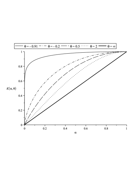
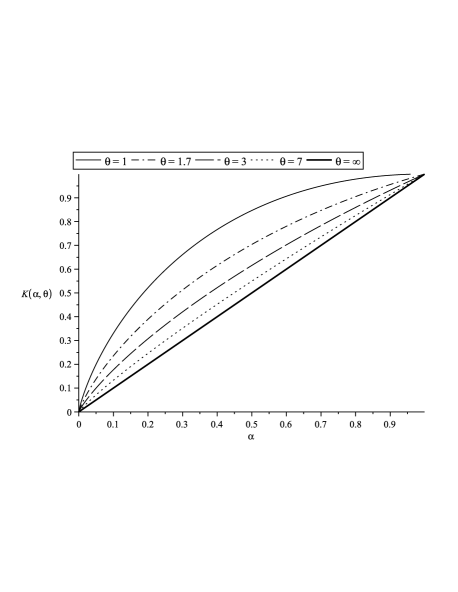
Figure 1: Kendall distribution $K(\cdot,\theta)$ for different values of $\theta$ in the Clayton copula case (left) and the Gumbel copula case (right). The dark full line represents the first diagonal and it corresponds to the comonotonic case.

2 Multivariate generalization of the Value-at-Risk measure

From the usual definition in the univariate setting, the Value-at-Risk is the minimal amount of the loss which accumulates a probability $\alpha$ to the left tail and $1-\alpha$ to the right tail. Then, if $F_{X}$ denotes the cumulative distribution function associated with risk $X$ and $\overline{F}_{X}$ its associated survival function, then

$${\rm VaR}_{\alpha}(X):=\inf\left\{x\in\mathbb{R}:F_{X}(x)\geq\alpha\right\}$$

and equivalently,

$${\rm VaR}_{\alpha}(X):=\inf\left\{x\in\mathbb{R}:\overline{F}_{X}(x)\leq 1-\alpha\right\}.$$

Consequently, the classical univariate VaR can be viewed as the boundary of the set $\left\{x\in\mathbb{R}:\right.$ $\left.F_{X}(x)\geq\alpha\right\}$ or, similarly, the boundary of the set $\left\{x\in\mathbb{R}:\overline{F}_{X}(x)\leq 1-\alpha\right\}$.

This idea can be easily extended in higher dimension, keeping in mind that the two previous sets are different in general as soon as $d\geq 2$. We propose a multivariate generalization of Value-at-Risk for a portfolio of $d$ dependent risks. As a starting point, we consider Definition 17 in Embrechts and Puccetti (2006). They suggest to define the multivariate lower-orthant Value-at-Risk at probability level $\alpha$, for a increasing function $\underline{G}$ : $\mathbb{R}^{d}\rightarrow[0,1]$, as the boundary of its $\alpha$–upper-level set, i.e., $\partial\{\textbf{x}\in\mathbb{R}^{d}:\underline{G}(\textbf{x})\geq\alpha\}$ and analogously, the multivariate upper-orthant Value-at-Risk, for a decreasing function $\overline{G}$ : $\mathbb{R}^{d}\rightarrow[0,1]$, as the boundary of its $(1-\alpha)$–lower-level set, i.e., $\partial\{\textbf{x}\in\mathbb{R}^{d}:\overline{G}(\textbf{x})\leq 1-\alpha\}$.

Note that the generalizations of Value-at-Risk by Embrechts and Puccetti (2006) (see also Nappo and Spizzichino, 2009; Tibiletti, 1993) are represented by an infinite number of points (an hyperspace of dimension $d-1$, under some regularly conditions on the functions $\underline{G}$ and $\overline{G}$). This choice can be unsuitable when we face real risk management problems. Then, we propose more parsimonious and synthetic versions of the Embrechts and Puccetti (2006)’s measures. In particular in our propositions, instead of considering the whole hyperspace $\partial\{\textbf{x}:\underline{G}(\textbf{x})\geq\alpha\}$ (or $\partial\{\textbf{x}:\overline{G}(\textbf{x})\leq 1-\alpha\}$) we only focus on the particular point in $\mathbb{R}_{+}^{d}$ that matches the conditional expectation of X given that X stands in this set. This means that our measures are real-valued vectors with the same dimension as the considered portfolio of risks.

In addition, to be consistent with the univariate definition of $\rm{VaR}$, we choose $\underline{G}$ (resp. $\overline{G}$) as the $d-$dimensional loss distribution function $F$ (resp. the survival distribution function $\overline{F}$) of the risk portfolio. This allows to capture information coming both from the marginal distributions and from the multivariate dependence structure, without using an arbitrary real-valued aggregate transformation (for more details see Introduction).

In analogy with the Embrechts and Puccetti’s notation we will denote $\underline{{\rm VaR}}$ our multivariate lower-orthant Value-at-Risk and $\overline{{\rm VaR}}$ the upper-orthant one.

In the following, we will consider non-negative absolutely-continuous random vector ${\textbf{X}=(X_{1},\ldots,X_{d})}$ (with respect to Lebesgue measure $\lambda$ on $\mathbb{R}^{d}$) with partially increasing multivariate distribution function $F$ and such that ${\operatorname{\mathbb{E}}(X_{i})<\infty},$ for $i=1,\ldots,d$. These conditions will be called regularity conditions.

However, extensions of our results in the case of multivariate distribution function on the entire space $\mathbb{R}^{d}$ or in the presence of plateau in the graph of $F$ are possible. Starting from these considerations, we introduce here a multivariate generalization of the VaR measure.

Definition 2.1 (Multivariate lower-orthant Value-at-Risk)

Consider a random vector $\textbf{X}=(X_{1},\ldots,X_{d})$ with distribution function $F$ satisfying the regularity conditions. For $\alpha\in(0,1)$, we define the multidimensional lower-orthant Value-at-Risk at probability level $\alpha$ by

$$\underline{{\rm VaR}}_{\alpha}(\textbf{X})=\operatorname{\mathbb{E}}[\textbf{X}|\,\textbf{X}\in\partial\underline{L}(\alpha)]=\left(\begin{array}[]{ll}\operatorname{\mathbb{E}}[\,X_{1}\,|\,\textbf{X}\in\partial\underline{L}(\alpha)\,]\vspace{0.04cm}\\ \quad\quad\quad\quad\vdots\vspace{0.04cm}\\ \operatorname{\mathbb{E}}[\,X_{d}\,|\,\textbf{X}\in\partial\underline{L}(\alpha)\,]\end{array}\right).$$

where $\partial\underline{L}(\alpha)$ is the boundary of the set $\underline{L}(\alpha):=\{\textbf{x}\in\mathbb{R}^{d}_{+}:F(\textbf{x})\geq\alpha\}$. Under the regularity conditions, $\partial\underline{L}(\alpha)$ is the $\alpha$-level set of $F$, i.e., $\partial\underline{L}(\alpha)=\{\textbf{x}\in\mathbb{R}^{d}_{+}:F(\textbf{x})=\alpha\}$ and the previous definition can be restated as

$$\underline{{\rm VaR}}_{\alpha}(\textbf{X})=\operatorname{\mathbb{E}}[\textbf{X}|\,F(\textbf{X})=\alpha]=\left(\begin{array}[]{ll}\operatorname{\mathbb{E}}[\,X_{1}\,|\,F(\textbf{X})=\alpha\,]\vspace{0.04cm}\\ \quad\quad\quad\quad\vdots\vspace{0.04cm}\\ \operatorname{\mathbb{E}}[\,X_{d}\,|\,F(\textbf{X})=\alpha\,]\end{array}\right).$$

Note that, under the regularity conditions, $\partial\underline{L}(\alpha)=\{\textbf{x}\in\mathbb{R}^{d}_{+}:F(\textbf{x})=\alpha\}$ has Lebesgue-measure zero in $\mathbb{R}^{d}_{+}$ (e.g., see Property 3 in Tibiletti, 1990). Then we make sense of Definition 2.1 using the limit procedure in Feller (1966), Section 3.2:

$$\operatorname{\mathbb{E}}[\,X_{i}\,|\,F(\textbf{X})=\alpha\,]=\lim_{h\rightarrow 0}\,\operatorname{\mathbb{E}}[\,X_{i}\,|\,\alpha<F(\textbf{X})\leq\alpha+h\,]\\ =\lim_{h\rightarrow 0}\,\frac{\int_{Q_{X_{i}}(\alpha)}^{\infty}x\left(\int_{\alpha}^{\alpha+h}f_{(X_{i},F(\textbf{X}))}(x,y)\,{\mathrm{d}}y\right){\mathrm{d}}x}{\int_{\alpha}^{\alpha+h}f_{F(\textbf{X})}(y)\,{\mathrm{d}}y},$$ (1)

for $i=1,\ldots,d$.

Dividing numerator and denominator in (1) by $h$, we obtain, as $h\rightarrow 0$

$$\operatorname{\mathbb{E}}[X_{i}\,|F(\textbf{X})=\alpha]=\frac{\int_{Q_{X_{i}}(\alpha)}^{\infty}x\,f_{(X_{i},F(\textbf{X}))}(x,\alpha)\,{\mathrm{d}}x}{K^{\prime}(\alpha)},$$ (2)

for $i=1,\ldots,d$, where $K^{\prime}(\alpha)=\frac{{\mathrm{d}}K(\alpha)}{{\mathrm{d}}\alpha}$ is the Kendall distribution density function. This procedure gives a rigorous sense to our $\underline{{\rm VaR}}_{\alpha}(\textbf{X})$ in Definition 2.1. Remark that the existence of $f_{(X_{i},F(\textbf{X}))}$ and $K^{\prime}$ in (2) is guaranteed by the regularity conditions (for further details, see Proposition 1 in Imlahi et al., 1999 or Proposition 4 in Chakak and Ezzerg, 2000).

In analogy with Definition 2.1, we now introduce another possible generalization of the VaR measure based on the survival distribution function.

Definition 2.2 (Multivariate upper-orthant Value-at-Risk)

Consider a random vector $\textbf{X}=(X_{1},\ldots,X_{d})$ with survival distribution $\overline{F}$ satisfying the regularity conditions. For $\alpha\in(0,1)$, we define the multidimensional upper-orthant Value-at-Risk at probability level $\alpha$ by

$$\overline{{\rm VaR}}_{\alpha}(\textbf{X})=\operatorname{\mathbb{E}}[\textbf{X}|\,\textbf{X}\in\partial\overline{L}(\alpha)]=\left(\begin{array}[]{ll}\operatorname{\mathbb{E}}[\,X_{1}\,|\,\textbf{X}\in\partial\overline{L}(\alpha)\,]\vspace{0.04cm}\\ \quad\quad\quad\quad\vdots\vspace{0.04cm}\\ \operatorname{\mathbb{E}}[\,X_{d}\,|\,\textbf{X}\in\partial\overline{L}(\alpha)\,]\end{array}\right).$$

where $\partial\overline{L}(\alpha)$ is the boundary of the set $\overline{L}(\alpha):=\{\textbf{x}\in\mathbb{R}^{d}_{+}:\overline{F}(\textbf{x})\leq 1-\alpha\}$. Under the regularity conditions, $\partial\overline{L}(\alpha)$ is the $(1-\alpha)$-level set of $\overline{F}$, i.e., $\partial\overline{L}(\alpha)=\{\textbf{x}\in\mathbb{R}^{d}_{+}:\overline{F}(\textbf{x})=1-\alpha\}$ and the previous definition can be restated as

$$\overline{{\rm VaR}}_{\alpha}(\textbf{X})=\operatorname{\mathbb{E}}[\textbf{X}|\,\overline{F}_{\textbf{X}}(\textbf{X})=1-\alpha]=\left(\begin{array}[]{ll}\operatorname{\mathbb{E}}[\,X_{1}\,|\,\overline{F}(\textbf{X})=1-\alpha\,]\vspace{0.04cm}\\ \quad\quad\quad\quad\vdots\vspace{0.04cm}\\ \operatorname{\mathbb{E}}[\,X_{d}\,|\,\overline{F}(\textbf{X})=1-\alpha\,]\end{array}\right).$$

As for $\partial\underline{L}(\alpha)$, under the regularity conditions, $\partial\overline{L}(\alpha)=\{\textbf{x}\in\mathbb{R}^{d}_{+}:\overline{F}(\textbf{x})=1-\alpha\}$ has Lebesgue-measure zero in $\mathbb{R}^{d}_{+}$ (e.g., see Property 3 in Tibiletti, 1990) and we make sense of Definition 2.2 using the limit Feller’s procedure (see Equations (1)-(2)).

From now on, we denote by $\underline{{\rm VaR}}^{1}_{\alpha}(\textbf{X})$, $\ldots$, $\underline{{\rm VaR}}^{d}_{\alpha}(\textbf{X})$ the components of the vector $\underline{{\rm VaR}}_{\alpha}(\textbf{X})$ and by $\overline{{\rm VaR}}^{1}_{\alpha}(\textbf{X})$, $\ldots$, $\overline{{\rm VaR}}^{d}_{\alpha}(\textbf{X})$ the components of the vector $\overline{{\rm VaR}}_{\alpha}(\textbf{X})$.

Note that if X is an exchangeable random vector, ${\underline{\mbox{VaR}}_{\alpha}^{i}(\textbf{X})=\underline{\mbox{VaR}}_{\alpha}^{j}(\textbf{X})}$ and ${\overline{\mbox{VaR}}_{\alpha}^{i}(\textbf{X})=\overline{\mbox{VaR}}_{\alpha}^{j}(\textbf{X})}$ for any $i,j=1,\ldots,d$. Furthermore, given a univariate random variable $X$, $\operatorname{\mathbb{E}}[X\,|F_{X}(X)=\alpha]=\operatorname{\mathbb{E}}[X\,|\overline{F}_{X}(X)=1-\alpha]=\rm{VaR}_{\alpha}(X),$ for all $\alpha$ in $(0,1)$. Hence, lower-orthant VaR and upper-orthant VaR are the same for (univariate) random variables and Definitions 2.1 and 2.2 can be viewed as natural multivariate versions of the univariate case. As remarked above, in Definitions 2.1-2.2 instead of considering the whole hyperspace $\partial\underline{L}(\alpha)$ (or $\partial\overline{L}(\alpha)$), we only focus on the particular point in $\mathbb{R}_{+}^{d}$ that matches the conditional expectation of X given that X falls in $\partial\underline{L}(\alpha)$ (or in $\partial\overline{L}(\alpha)$).

2.1 Invariance properties

In the present section, the aim is to analyze the lower-orthant VaR and upper-orthant VaR introduced in Definitions 2.1-2.2 in terms of classical invariance properties of risk measures (we refer the interested reader to Artzner et al., 1999). As these measures are not the same in general for dimension greater or equal to $2$, we also provide some connections between these two measures.

We now introduce the following results (Proposition 2.1 and Corollary 2.1) that will be useful in order prove invariance properties of our risk measures.

Proposition 2.1

Let the function $h$ be such that $h(x_{1},\ldots,x_{d})=(h_{1}(x_{1}),\ldots,h_{d}(x_{d}))$.

• If $h_{1},\ldots,h_{d}$ are non-decreasing functions, then the following relations hold

  $$\underline{{\rm VaR}}^{i}_{\alpha}(h(\textbf{X}))=\operatorname{\mathbb{E}}[\,h_{i}(X_{i})\,|\,F_{\textbf{X}}(\textbf{X})=\alpha\,],\;\;i=1,\ldots,d.$$

• If $h_{1},\ldots,h_{d}$ are non-increasing functions, then the following relations hold

  $$\underline{{\rm VaR}}^{i}_{\alpha}(h(\textbf{X}))=\operatorname{\mathbb{E}}[\,h_{i}(X_{i})\,|\,\overline{F}_{\textbf{X}}(\textbf{X})=\alpha\,],\;\;i=1,\ldots,d.$$

Proof: From Definition 2.1, $\underline{{\rm VaR}}^{i}_{\alpha}(h(\textbf{X}))=\operatorname{\mathbb{E}}[\,h_{i}(X_{i})\,|\,{F}_{h(\textbf{X})}(h(\textbf{X}))=\alpha\,]$, for $i=1,\ldots,d$. Since

$$F_{h(\textbf{X})}(y_{1},\ldots,y_{d})=\left\{\begin{array}[]{ll}F_{\textbf{X}}(h^{-1}(y_{1}),\ldots,h^{-1}(y_{d})),&\mbox{ if }h_{1},\ldots,h_{d}\mbox{ are non-decreasing functions,}\\ \overline{F}_{\textbf{X}}(h^{-1}(y_{1}),\ldots,h^{-1}(y_{d})),&\mbox{ if }h_{1},\ldots,h_{d}\mbox{ are non-increasing functions,}\end{array}\right.$$

then we obtain the result. $\Box$

From Proposition 2.1 one can trivially obtain the following property which links the multivariate upper-orthant Value-at-Risk and lower-orthant one.

Corollary 2.1

Let $h$ be a linear function such that $h(x_{1},\ldots,x_{d})=(h_{1}(x_{1}),\ldots,h_{d}(x_{d}))$.

• If $h_{1},\ldots,h_{d}$ are non-decreasing functions then then it holds that

  $\underline{{\rm VaR}}_{\alpha}(h(\textbf{X}))=h(\underline{{\rm VaR}}_{\alpha}(\textbf{X}))\quad$ and $\quad\overline{{\rm VaR}}_{\alpha}(h(\textbf{X}))=h(\overline{{\rm VaR}}_{\alpha}(\textbf{X}))$.

• If $h_{1},\ldots,h_{d}$ are non-increasing functions then it holds that

  $\underline{{\rm VaR}}_{\alpha}(h(\textbf{X}))=h(\overline{{\rm VaR}}_{1-\alpha}(\textbf{X}))\quad$ and $\quad\overline{{\rm VaR}}_{\alpha}(h(\textbf{X}))=h(\underline{{\rm VaR}}_{1-\alpha}(\textbf{X}))$.

Example 1

If $X=(X_{1},\ldots,X_{d})$ is a random vector with uniform margins and if, for all $i=1,\ldots,d$, we consider the functions $h_{i}$ such that $h_{i}(x)=1-x$, $x\in[0,1]$, then from Corollary 2.1,

$$\overline{{\rm VaR}}^{i}_{\alpha}(\textbf{X})=1-\underline{{\rm VaR}}^{i}_{1-\alpha}(\textbf{1}-\textbf{X})$$ (3)

for all $i=1,\ldots,d$, where $\textbf{1}-\textbf{X}=(1-X_{1},\ldots,1-X_{d})$. In this case, $\overline{{\rm VaR}}_{\alpha}(\textbf{X})$ is the point reflection of $\,\underline{{\rm VaR}}_{1-\alpha}({\rm\textbf{1}}-\textbf{X})$ with respect to point $\mathcal{I}$ with coordinates $(\frac{1}{2},\ldots,\frac{1}{2})$. If X and $\textbf{1}-\textbf{X}$ have the same distribution function, then $X$ is invariant in law by central symmetry and additionally the copula of $X$ and its associated survival copula are the same. In that case $\overline{{\rm VaR}}_{\alpha}(\textbf{X})$ is the point reflection of $\underline{{\rm VaR}}_{1-\alpha}(\textbf{X})$ with respect to $\mathcal{I}$. This property holds for instance for elliptical copulas or for the Frank copula.

Finally, we can state the following result that proves positive homogeneity and translation invariance for our measures.

Proposition 2.2

Consider a random vector X satisfying the regularity conditions. For $\alpha\in(0,1)$, the multivariate upper-orthant and lower-orthant Value-at-Risk satisfiy the following properties:

Positive Homogeneity: $\quad\forall\,\,\,\textbf{c}\in\mathbb{R}^{d}_{+},$

$$\underline{{\rm VaR}}_{\alpha}(\textbf{c}\textbf{X})=\textbf{c}\underline{{\rm VaR}}_{\alpha}(\textbf{X}),\quad\overline{{\rm VaR}}_{\alpha}(\textbf{c}\textbf{X})=\textbf{c}\overline{{\rm VaR}}_{\alpha}(\textbf{X})$$

Translation Invariance: $\quad\forall\,\,\,\textbf{c}\in\mathbb{R}^{d}_{+},$

$$\underline{{\rm VaR}}_{\alpha}(\textbf{c}+\textbf{X})=\textbf{c}+\underline{{\rm VaR}}_{\alpha}(\textbf{X}),\quad\overline{{\rm VaR}}_{\alpha}(\textbf{c}+\textbf{X})=\textbf{c}+\overline{{\rm VaR}}_{\alpha}(\textbf{X})$$

The proof comes down from Corollary 2.1.

2.2 Archimedean copula case

Surprisingly enough, the VaR and $\overline{{\rm VaR}}$ introduced in Definitions 2.1-2.2 can be computed analytically for any $d-$dimensional random vector with an Archimedean copula dependence structure. This is due to McNeil and Nešlehová’s stochastic representation of Archimedean copulas.

Proposition 2.3

(McNeil and Nešlehová, 2009) Let $\textbf{U}=(U_{1},\ldots,U_{d})$ be distributed according to a $d$-dimensional Archimedian copula with generator $\phi$, then

$$\left(\phi(U_{1}),\ldots,\phi(U_{d})\right)\stackrel{{\scriptstyle d}}{{=}}R\textbf{S}\,,$$ (4)

where $\textbf{S}=(S_{1},\ldots,S_{d})$ is uniformly distributed on the unit simplex $\left\{\textbf{x}\geq 0\mid\sum_{k=1}^{d}x_{k}=1\right\}$ and $R$ is an independent non-negative scalar random variable which can be interpreted as the radial part of $\left(\phi(U_{1}),\ldots,\phi(U_{d})\right)$ since $\sum_{k=1}^{d}S_{k}=1$. The random vector S follows a symmetric Dirichlet distribution whereas the distribution of $R\stackrel{{\scriptstyle d}}{{=}}\sum_{k=1}^{d}\phi(U_{k})$ is directly related to the generator $\phi$ through the inverse Williamson transform of $\phi^{-1}.$

Recall that a $d$-dimensional Archimedean copula with generator $\phi$ is defined by $C(u_{1},\ldots,u_{d})=\phi^{-1}(\phi(u_{1})+\cdots+\phi(u_{d}))$, for all $(u_{1},\ldots,u_{d})\in[0,1]^{d}.$ Then, the radial part $R$ of representation (4) is directly related to the generator $\phi$ and the probability integral transformation of U, that is,

$$R\stackrel{{\scriptstyle d}}{{=}}\phi(C(\textbf{U})).$$

As a result, any random vector $\textbf{U}=\left(U_{1},\ldots,U_{d}\right)$ which follows an Archimedean copula with generator $\phi$ can be represented as a deterministic function of $C(\textbf{U})$ and an independent random vector $\textbf{S}=(S_{1},\ldots,S_{d})$ uniformly distributed on the unit simplex, i.e.,

$$\left(U_{1},\ldots,U_{d}\right)\stackrel{{\scriptstyle d}}{{=}}\left(\phi^{-1}\left(S_{1}\phi\left(C(\textbf{U})\right)\right),\ldots,\phi^{-1}\left(S_{d}\phi\left(C(\textbf{U})\right)\right)\right).$$ (5)

The previous relation allows us to obtain an easily tractable expression of $\underline{{\rm VaR}}_{\alpha}(\textbf{X})$ for any random vector X with an Archimedean copula dependence structure.

Corollary 2.2

Let X be a $d$-dimensional random vector with marginal distributions $F_{1},\ldots,F_{d}$. Assume that the dependence structure of X is given by an Archimedian copula with generator $\phi$. Then, for any $i=1,\ldots,d,$

$$\underline{{\rm VaR}}_{\alpha}^{i}(\textbf{X})=\operatorname{\mathbb{E}}\left[F_{i}^{-1}\left(\phi^{-1}(S_{i}\phi(\alpha))\right)\right]$$ (6)

where $S_{i}$ is a random variable with ${\rm Beta}(1,d-1)$ distribution.

Proof: Note that X is distributed as $(F_{1}^{-1}(U_{1}),\ldots,F_{d}^{-1}(U_{d}))$ where $\textbf{U}=(U_{1},\ldots,U_{d})$ follows an Archimedean copula $C$ with generator $\phi$. Then, each component $i=1,\ldots,d\,$ of the multivariate risk measure introduced in Definition 2.1 can be expressed as $\underline{{\rm VaR}}_{\alpha}^{i}(\textbf{X})=\operatorname{\mathbb{E}}\left[F_{i}^{-1}(U_{i})\mid C(\textbf{U})=\alpha\right]$. Moreover, from representation (5) the following relation holds

$$\left[\textbf{U}\mid C(\textbf{U})=\alpha\right]\stackrel{{\scriptstyle d}}{{=}}\left(\phi^{-1}\left(S_{1}\phi\left(\alpha\right)\right),\ldots,\phi^{-1}\left(S_{d}\phi\left(\alpha\right)\right)\right)$$ (7)

since S and $C(\textbf{U})$ are stochastically independent. The result comes down from the fact that the random vector $(S_{1},\ldots,S_{d})$ follows a symmetric Dirichlet distribution. $\Box$

Note that, using (7), the marginal distributions of U given $C(\textbf{U})=\alpha$ can be expressed in a very simple way, that is, for any $k=1,\ldots,d,$

$$\mathbb{P}(U_{k}\leq u\mid C(\textbf{U})=\alpha)=\left(1-\frac{\phi(u)}{\phi(\alpha)}\right)^{d-1}\,\,\quad\mbox{ for }\,\,0<\alpha<u<1.$$ (8)

The latter relation derives from the fact that $S_{k},$ which is ${\rm Beta}(1,d-1)$- distributed, is such that $S_{k}\stackrel{{\scriptstyle d}}{{=}}1-V^{\frac{1}{d-1}}$ where $V$ is uniformly-distributed on $(0,1)$.

We now adapt Corollary 2.2 for the multivariate upper-orthant Value-at-Risk, i.e., $\overline{{\rm VaR}}_{\alpha}$.

Corollary 2.3

Let X be a $d$-dimensional random vector with marginal survival distributions $\overline{F}_{1},\ldots,\overline{F}_{d}$. Assume that the survival copula of X is an Archimedean copula with generator $\phi$. Then, for any $i=1,\ldots,d,$

$$\overline{{\rm VaR}}_{\alpha}^{i}(\textbf{X})=\operatorname{\mathbb{E}}\left[\overline{F}_{i}^{-1}\left(\phi^{-1}(S_{i}\phi(1-\alpha))\right)\right]$$ (9)

where $S_{i}$ is a random variable with ${\rm Beta}(1,d-1)$ distribution.

Proof: Note that X is distributed as $(\overline{F}_{1}^{-1}(U_{1}),\ldots,\overline{F}_{d}^{-1}(U_{d}))$ where $\textbf{U}=(U_{1},\ldots,U_{d})$ follows an Archimedean copula $\overline{C}$ with generator $\phi$. Then, each component $i=1,\ldots,d\,$ of the multivariate risk measure introduced in Definition 2.2 can be expressed as $\overline{{\rm VaR}}_{\alpha}^{i}(\textbf{X})=\operatorname{\mathbb{E}}\left[\overline{F}_{i}^{-1}(U_{i})\mid\overline{C}(\textbf{U})=1-\alpha\right]$. Then, relation 7 also holds for $\mathbf{{U}}$ and $\overline{C}$, i.e., $\left[\textbf{U}\mid\overline{C}(\textbf{U})=1-\alpha\right]\stackrel{{\scriptstyle d}}{{=}}\left(\phi^{-1}\left(S_{1}\phi\left(1-\alpha\right)\right),\ldots,\phi^{-1}\left(S_{d}\phi\left(1-\alpha\right)\right)\right)$. Hence the result. $\Box$

In the following, from (6) and (9), we derive analytical expressions of the lower-orthant and the upper-orthant Value-at-Risk for a random vector $\mathbf{X}=(X_{1},\ldots,X_{d})$ distributed as a particular Archimedean copula. Let us first remark that , as Archimedean copulas are exchangeable, the components of $\underline{\rm{VaR}}$ (resp. $\overline{\rm{VaR}}$) are the same. Moreover, as far as closed-form expressions are available for the lower-orthant $\underline{\rm{VaR}}$ of $\mathbf{X}$, it is also possible to derive an analogue expression for the upper-orthant $\overline{\rm{VaR}}$ of $\mathbf{\tilde{X}}=(1-X_{1},\ldots,1-X_{d})$ since from Example 1

$$\overline{{\rm VaR}}^{i}_{\alpha}(\mathbf{\tilde{X}})=1-\underline{{\rm VaR}}^{i}_{1-\alpha}(\mathbf{X}).$$ (10)

Clayton family in dimension $2$:

As a matter of example, let us now consider the Clayton family of bivariate copulas. This family is interesting since it contains the counter-monotonic, the independence and the comonotonic copulas as particular cases. Let $(X,Y)$ be a random vector distributed as a Clayton copula with parameter $\theta\geq-1$. Then, $X$ and $Y$ are uniformly-distributed on $(0,1)$ and the joint distribution function $C_{\theta}$ of $(X,Y)$ is such that

$$C_{\theta}(x,y)=(\max\{x^{-\theta}+y^{-\theta}-1,0\})^{-\frac{1}{\theta}},\quad\mbox{ for }\theta\geq-1,\,\,\,\,\,(x,y)\in[0,1]^{2}.$$ (11)

Table 3 gives analytical expressions for the first (equal to the second) component of $\underline{\rm{VaR}}$ as a function of the risk level $\alpha$ and the dependence parameter $\theta$. For $\theta=-1$ and $\theta=\infty$ we obtain the Fréchet-Hoeffding lower and upper bounds: $W(x,y)=\max\{x+y-1,0\}$ (counter-monotonic copula) and $M(x,y)=\min\{x,y\}$ (comonotonic random copula) respectively. The settings $\theta=0$ and $\theta=1$ correspond to degenerate cases. For $\theta=0$ we have the independence copula $\Pi(x,y)=x\,y$. For $\theta=1$, we obtain the copula denoted by $\frac{\Pi}{\Sigma-\Pi}$ in Nelsen (1999), where $\frac{\Pi}{\Sigma-\Pi}(x,y)=\frac{x\,y}{x+y-x\,y}$.

Copula	$\theta$	$\underline{{\rm VaR}}^{1}_{\alpha,\theta}(X,Y)$
Clayton $C_{\theta}$	$(-1,\infty)$	$\frac{\theta}{\theta-1}{\frac{{\alpha}^{\theta}-\alpha}{{\alpha}^{\theta}-1}}$
Counter-monotonic $W$	$-1$	$\frac{1+\alpha}{2}$
Independent $\Pi$	$0$	${\frac{\alpha-1}{\ln\alpha}}$
$\frac{\Pi}{\Sigma-\Pi}$	$1$	${\frac{\alpha\,\ln\alpha}{\alpha-1}}$
Comonotonic $M$	$\infty$	$\alpha$

Table 3: $\underline{{\rm VaR}}^{1}_{\alpha,\theta}(X,Y)$ for different dependence structures.

Interestingly, one can readily show that $\frac{\partial\underline{{\rm VaR}}^{1}_{\alpha,\theta}}{\partial\alpha}\geq 0$ and $\frac{\partial\underline{{\rm VaR}}^{1}_{\alpha,\theta}}{\partial\theta}\leq 0$, for $\theta\geq-1$ and $\alpha\in(0,1)$. This proves that, for Clayton-distributed random couples, the components of our multivariate VaR are increasing functions of the risk level $\alpha$ and decreasing functions of the dependence parameter $\theta$. Note also that the multivariate VaR in the comonotonic case corresponds to the vector composed of the univariate VaR associated with each component. These properties are illustrated in Figure 2 (left) where $\underline{{\rm VaR}}^{1}_{\alpha,\theta}(X,Y)$ is plotted as a function of the risk level $\alpha$ for different values of the parameter $\theta$. Observe that an increase of the dependence parameter $\theta$ tends to lower the VaR up to the perfect dependence case where $\underline{{\rm VaR}}_{\alpha,\theta}^{1}(X,Y)=\underline{{\rm VaR}}_{\alpha}(X)=\alpha$. The latter empirical behaviors will be formally confirmed in next sections.

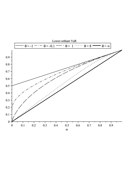
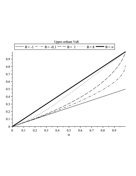
Figure 2: Behavior of $\underline{{\rm VaR}}^{1}_{\alpha,\theta}(X,Y)=\underline{{\rm VaR}}^{2}_{\alpha,\theta}(X,Y)$ (left) and $\overline{{\rm VaR}}^{1}_{\alpha,\theta}(1-X,1-Y)=\overline{{\rm VaR}}^{2}_{\alpha,\theta}(1-X,1-Y)$ (right) with respect to risk level $\alpha$ for different values of dependence parameter $\theta$. The random vector $(X,Y)$ follows a Clayton copula distribution with parameter $\theta$. Note that, due to Equation 10, the two graphs are symmetric with respect to the point $(\frac{1}{2},\frac{1}{2})$

In the same framework, using Equation 10, one can readily show that $\frac{\partial\overline{{\rm VaR}}^{1}_{\alpha,\theta}}{\partial\alpha}\geq 0$ and $\frac{\partial\overline{{\rm VaR}}^{1}_{\alpha,\theta}}{\partial\theta}\geq 0$, for $\theta\geq-1$ and $\alpha\in(0,1)$. This proves that, for random couples with uniform margins and Clayton survival copula, the components of our multivariate $\overline{{\rm VaR}}$ are increasing functions both of the risk level $\alpha$ and of the dependence parameter $\theta$. Note also that the multivariate $\overline{{\rm VaR}}$ in the comonotonic case corresponds to the vector composed of the univariate VaR associated with each component. These properties are illustrated in Figure 2 (right) where $\overline{{\rm VaR}}^{1}_{\alpha,\theta}(X,Y)$ is plotted as a function of the risk level $\alpha$ for different values of the parameter $\theta$. Observe that, contrary to the lower-orthant $\underline{\rm{VaR}}$, an increase of the dependence parameter $\theta$ tends to increase the $\overline{{\rm VaR}}$. The upper bound is represented by the perfect dependence case where $\overline{{\rm VaR}}_{\alpha,\theta}^{1}(X,Y)={\rm VaR}_{\alpha}(X)=\alpha$. The latter empirical behaviors will be formally confirmed in next sections.

Ali-Mikhail-Haq in dimension $2$:

Let $(X,Y)$ be a random vector distributed as a Ali-Mikhail-Haq copula with parameter $\theta\in[-1,1)$. In particular, the marginal distribution of $X$ and $Y$ are uniform. Then, the distribution function $C_{\theta}$ of $(X,Y)$ is such that

$$C_{\theta}(x,y)=\frac{x\,y}{1-\theta\,(1-x)(1-y)},\quad\mbox{ for }\theta\in[-1,1),\,\,\,\,\,(x,y)\in[0,1]^{2}.$$

Using Corollary 2.2, we give in Table 4 analytical expressions for the first (equal to the second) component of the $\underline{{\rm VaR}}$, i.e., $\underline{{\rm VaR}}^{1}_{\alpha,\theta}(X,Y)$. When $\theta=0$ we obtain the independence copula $\Pi(x,y)=x\,y$.

Copula	$\theta$	$\underline{{\rm VaR}}^{1}_{\alpha,\theta}(X,Y)$
Ali-Mikhail-Haq copula $C_{\theta}$	$[-1,1)$	${\frac{\left(\theta-1\right)\ln\left(1-\theta(1-\alpha)\right)}{\theta\left(\ln\left(1-\theta(1-\alpha)\right)-\ln\left(\alpha\right)\right)}}$
Independent $\Pi$	$0$	${\frac{\alpha-1}{\ln\left(\alpha\right)}}$

Table 4: $\underline{{\rm VaR}}^{1}_{\alpha,\theta}(X,Y)$ for a bivariate Ali-Mikhail-Haq copula.

Clayton family in dimension $3$:

We now consider a $3$-dimensional vector $\textbf{X}=(X_{1},X_{2},X_{3})$ with Clayton copula and parameter $\theta>-\frac{1}{2}$ (see Remark 1) and uniform marginals. In this case we give an analytical expression of $\underline{{\rm VaR}}^{i}_{\alpha,\theta}(X_{1},X_{2},X_{3})$ for $i=1,2,3$. Results are given in Table 5.

Copula	$\theta$	$\underline{{\rm VaR}}^{i}_{\alpha,\theta}(X_{1},X_{2},X_{3})$
Clayton $C_{\theta}$	$(-1/2,\infty)$	$2\,{\frac{\theta\,\left((\theta-1){\alpha}^{2\,\theta}+(1-2\theta){\alpha}^{\theta}+\theta\alpha\right)}{\left(2\,\theta-1\right)\left(\theta-1\right)\left({\alpha}^{2\,\theta}-2\,{\alpha}^{\theta}+1\right)}}$
Independent $\Pi$	$0$	$-2\,{\frac{1-\alpha+\ln\left(\alpha\right)}{\left(\ln\left(\alpha\right)\right)^{2}}}$

Table 5: $\underline{{\rm VaR}}^{1}_{\alpha,\theta}(X_{1},X_{2},X_{3})$ for different dependence structures.

As in the bivariate case above, one can readily show that $\frac{\partial\underline{{\rm VaR}}^{1}_{\alpha,\theta}}{\partial\alpha}\geq 0,$ $\frac{\partial\underline{{\rm VaR}}^{1}_{\alpha,\theta}}{\partial\theta}\leq 0$ when $\mathbf{X}$ is distributed as a $3-$dimensional Clayton copula. In addition, using Equation 10, $\frac{\partial\overline{{\rm VaR}}^{1}_{\alpha,\theta}}{\partial\alpha}\geq 0$ and $\frac{\partial\overline{{\rm VaR}}^{1}_{\alpha,\theta}}{\partial\theta}>0$ when $\mathbf{X}$ admits a trivariate Clayton survival copula. Then, the results obtained above in the bivariate case are confirmed also in higher dimension. These empirical behaviors will be formally confirmed in next sections.

2.3 Comparison of univariate and multivariate VaR

Note that, using a change of variable, each component of the multivariate VaR can be represented as an integral transformation of the associated univariate VaR. Let us denote by $F_{X_{i}}$ the marginal distribution functions of $X_{i}$ for $i=1,\ldots,d$ and by $C$ (resp. $\overline{C}$) the copula (resp. the survival copula) associated with X. Using the Sklar’s theorem we have $F(x_{1},\ldots,x_{d})=C(F_{X_{1}}(x_{1}),\ldots,F_{X_{d}}(x_{d}))$ (see Sklar, 1959). Then the random variables $U_{i}$ defined by $U_{i}=F_{X_{i}}(X_{i})$, for $i=1,\ldots,d$, are uniformly distributed and their joint distribution is equal to $C$. Using these notations and since $F^{-1}_{X_{i}}(\gamma)={\rm VaR}_{\gamma}(X_{i})$, we get

$$\underline{{\rm VaR}}_{\alpha}^{i}(\textbf{X})=\frac{1}{K^{\prime}(\alpha)}\int_{\alpha}^{1}{\rm VaR}_{\gamma}(X_{i})f_{(U_{i},C(\textbf{U}))}(\gamma,\alpha)\,d\gamma,$$ (12)

for $i=1,\ldots,d,$ where $K^{\prime}$ is the density of the Kendall distribution associated with copula $C$ and $f_{(U_{i},C(\textbf{U}))}$ is the density function of the bivariate vector $(U_{i},C(\textbf{U}))$.

As for the upper-orthant VaR, let $V_{i}=\overline{F}_{X_{i}}(X_{i})$, for $i=1,\ldots,d$. Using these notations and since $\overline{F}^{-1}_{X_{i}}(\gamma)={\rm VaR}_{1-\gamma}(X_{i})$, we get

$$\overline{{\rm VaR}}_{\alpha}^{i}(\textbf{X})=\frac{1}{K^{\prime}_{\overline{C}}(1-\alpha)}\int_{0}^{1-\alpha}{\rm VaR}_{1-\gamma}(X_{i})f_{(V_{i},\overline{C}(\textbf{V}))}(\gamma,1-\alpha)\,d\gamma,$$ (13)

for $i=1,\ldots,d$, where $K^{\prime}_{\overline{C}}$ the density of the Kendall distribution associated with the survival copula $\overline{C}$ and $f_{(V_{i},\overline{C}(\textbf{V}))}$ is the density function of the bivariate vector $(V_{i},\overline{C}(\textbf{V}))$.

Remark that the bounds of integration in (12) and (13) derive from the geometrical properties of the considered level curve, i.e., $\partial\underline{L}(\alpha)$ (resp. $\partial\overline{L}(\alpha)$) is inferiorly (resp. superiorly) bounded by the marginal univariate quantile functions at level $\alpha$.

The following proposition allows us to compare the multivariate lower-orthant and upper-orthant Value-at-Risk with the corresponding univariate VaR.

Proposition 2.4

Consider a random vector X satisfying the regularity conditions. Assume that its multivariate distribution function $F$ is quasi concave. Then, for all $\,\alpha\in(0,1),$ the following inequalities hold

$$\overline{{\rm VaR}}^{i}_{\alpha}(\textbf{X})\leq{\rm VaR}_{\alpha}(X_{i})\leq\underline{{\rm VaR}}^{i}_{\alpha}(\textbf{X}),$$ (14)

for $i=1,\ldots,d$.

Proof: Let $\alpha\,\in\,(0,1)$. From the definition of the accumulated probability, it is easy to show that $\partial\underline{L}(\alpha)$ is inferiorly bounded by the marginal univariate quantile functions. Moreover, recall that $\underline{L}(\alpha)$ is a convex set in $\mathbb{R}^{d}_{+}$ from the quasi concavity of $F$ (see Section 2 in Tibiletti, 1995). Then, for all $\textbf{x}=(x_{1},\ldots,x_{d})\in\partial\underline{L}(\alpha)$, $x_{1}\geq\underline{{\rm VaR}}_{\alpha}(X_{1}),\cdots,x_{d}\geq\underline{{\rm VaR}}_{\alpha}(X_{d})$ and trivially, $\underline{{\rm VaR}}^{i}_{\alpha}(\textbf{X})$ is greater than ${\rm VaR}_{\alpha}(X_{i})$, for $i=1,\ldots,d$. Then $\underline{{\rm VaR}}^{i}_{\alpha}(\textbf{X})\geq{\rm VaR}_{\alpha}(X_{i})$, for all $\,\alpha\in(0,1)$ and $i=1,\ldots,d$. Analogously, from the definition of the survival accumulated probability, it is easy to show that $\partial\overline{L}(\alpha)$ is superiorly bounded by the marginal univariate quantile functions at level $\alpha$. Moreover, recall that $\overline{L}(\alpha)$ is a convex set in $\mathbb{R}^{d}_{+}$. Then, for all $\textbf{x}=(x_{1},\ldots,x_{d})\in\partial\overline{L}(\alpha)$, $x_{1}\leq{{\rm VaR}}_{\alpha}(X_{1}),\cdots,x_{d}\leq{{\rm VaR}}_{\alpha}(X_{d})$ and trivially, $\overline{{\rm VaR}}^{i}_{\alpha}(\textbf{X})$ is smaller than ${\rm VaR}_{\alpha}(X_{i})$, for all $\,\alpha\in(0,1)$ and $i=1,\ldots,d$. Hence the result $\Box$

Proposition 2.4 states that the multivariate lower-orthant $\underline{{\rm VaR}}_{\alpha}(\textbf{X})$ (resp. the multivariate upper-orthant $\overline{{\rm VaR}}_{\alpha}(\textbf{X})$) is more conservative (resp. less conservative) than the vector composed of the univariate $\alpha$-Value-at-Risk of marginals. Furthermore, we can prove that the previous bounds in (14) are reached for comonotonic random vectors.

Proposition 2.5

Consider a comonotonic non-negative random vector X. Then, for all $\,\alpha\in(0,1),$ it holds that

$$\overline{{\rm VaR}}^{i}_{\alpha}(\textbf{X})={\rm VaR}_{\alpha}(X_{i})=\underline{{\rm VaR}}^{i}_{\alpha}(\textbf{X}),$$

for $i=1,\ldots,d$.

Proof: Let $\alpha\,\in\,(0,1)$. If $\textbf{X}=(X_{1},\ldots,X_{d})$ is a comonotonic non-negative random vector then there exists a random variable $Z$ and $d$ increasing functions $g_{1},\ldots,g_{d}$ such that X is equal to $(g_{1}(Z),\ldots,g_{d}(Z))$ in distribution. So the set $\{(x_{1},\ldots,x_{d}):F(x_{1},\ldots,x_{d})=\alpha\}$ becomes $\{(x_{1},\ldots,x_{d}):$ $\min\{g^{-1}_{1}(x_{1}),\ldots,g^{-1}_{d}(x_{d})\}$ $=Q_{Z}(\alpha)\},$ where $Q_{Z}$ is the quantile function of $Z$. So, trivially, $\underline{{\rm VaR}}^{i}_{\alpha}(\textbf{X})=\operatorname{\mathbb{E}}[\,X_{i}\,|\,F(\textbf{X})=\alpha\,]=Q_{X_{i}}(\alpha)$, for $i=1,\ldots,d$ and $\overline{{\rm VaR}}^{i}_{\alpha}(\textbf{X})=\operatorname{\mathbb{E}}[g_{i}(Z)|\overline{F}_{\textbf{X}}(\textbf{X})=1-\alpha]=\operatorname{\mathbb{E}}[g_{i}(Z)|\overline{F}_{(Z,\ldots,Z)}(Z,\ldots,Z)=1-\alpha]$. Since $\overline{F}_{(Z,\ldots,Z)}(u_{1},\ldots,u_{d})=\overline{F}_{Z}(\max_{i=1,\ldots,d}u_{i}),$ then $\overline{{\rm VaR}}^{i}_{\alpha}(\textbf{X})=\operatorname{\mathbb{E}}[g_{i}(Z)|\overline{F}_{Z}(Z)=\alpha]={\rm VaR}_{\alpha}(X_{i}),$ for $i=1,\ldots,d$. Hence the result. $\Box$

Remark 3

For bivariate independent random couple $(X,Y)$, Equations (12) and (13) become respectivley

$$\underline{{\rm VaR}}_{\alpha}^{1}(X,Y) = \frac{1}{-\ln(\alpha)}\int_{\alpha}^{1}\frac{{\rm VaR}_{\gamma}(X)}{\gamma}\,d\gamma,$$

$$\overline{{\rm VaR}}_{\alpha}^{1}(X,Y) = \frac{1}{-\ln(1-\alpha)}\int_{0}^{1-\alpha}\frac{{\rm VaR}_{1-\gamma}(X)}{\gamma}\,d\gamma,$$

then, obviously, in this case the $X$-related component only depends on the marginal behavior of $X$. For further details the reader is referred to Corollary 4.3.5 in Nelsen (1999).

2.4 Behavior of the multivariate VaR with respect to marginal distributions

In this section we study the behavior of our VaR measures with respect to a change in marginal distributions. Results presented below provide natural multivariate extensions of some classical results in the univariate setting (see, e.g., Denuit and Charpentier, 2004).

Proposition 2.6

Let X and Y be two $d$–dimensional continuous random vectors satisfying the regularity conditions and with the same copula $C$. If $X_{i}\buildrel d\over{=}Y_{i}$ then it holds that

$$\underline{{\rm VaR}}^{i}_{\alpha}(\textbf{X})=\underline{{\rm VaR}}^{i}_{\alpha}(\textbf{Y}),\quad\mbox{ for all }\alpha\in(0,1),$$

and

$$\overline{{\rm VaR}}^{i}_{\alpha}(\textbf{X})=\overline{{\rm VaR}}^{i}_{\alpha}(\textbf{Y}),\quad\mbox{ for all }\alpha\in(0,1).$$

The proof of the previous result directly comes down from Equation (12) and (13). From Proposition 2.6, we remark that, for a fixed copula $C$, the $i$-th component $\underline{{\rm VaR}}_{\alpha}^{i}(\textbf{X})$ and $\overline{{\rm VaR}}^{i}_{\alpha}(\textbf{X})$ do not depend on marginal distributions of the other components $j$ with $j\neq i$.

In order to derive the next result, we use the definitions of stochastic orders presented in Section 1.

Proposition 2.7

Let X and Y be two $d$–dimensional continuous random vectors satisfying the regularity conditions and with the same copula $C$. If $X_{i}\preceq_{st}Y_{i}$ then it holds that

$$\underline{{\rm VaR}}^{i}_{\alpha}(\textbf{X})\leq\underline{{\rm VaR}}^{i}_{\alpha}(\textbf{Y}),\quad\mbox{ for all }\alpha\in(0,1),$$

and

$$\overline{{\rm VaR}}^{i}_{\alpha}(\textbf{X})\leq\overline{{\rm VaR}}^{i}_{\alpha}(\textbf{Y}),\quad\mbox{ for all }\alpha\in(0,1).$$

Proof: The proof comes down from formulas (12)- (13) and Definition 1.1. Furtheremore, we remark that if $X_{i}\preceq_{st}Y_{i}$ then ${F}^{-1}_{X_{i}}(x)\leq{F}^{-1}_{Y_{i}}(x)$ for all $x$, and $\overline{F}^{-1}_{X_{i}}(y)\leq\overline{F}^{-1}_{Y_{i}}(y)$ for all $y$. Hence the result. $\Box$

Note that, the result in Proposition 2.7 is consistent with the one-dimensional setting (see Section 3.3.1 in Denuit et al., 2005). Indeed, as in dimension one, an increase of marginals with respect to the first order stochastic dominance yields an increase in the corresponding components of ${\rm VaR}_{\alpha}(\textbf{X})$.

As a result, in an economy with several interconnected financial institutions, capital required for one particular institution is affected by its own marginal risk. But, for a fixed dependence structure, the solvency capital required for this specific institution does not depend on marginal risks bearing by the others. Then, our multivariate VaR implies a “fair” allocation of solvency capital with respect to individual risk-taking behavior. In other words, individual financial institutions may not have to pay more for risky business activities undertook by the others.

2.5 Behavior of multivariate VaR with respect to the dependence structure

In this section we study the behavior of our VaR measures with respect to a variation of the dependence structure, with unchanged marginal distributions.

Proposition 2.8

Let X and $\textbf{X}^{*}$ be two $d$–dimensional continuous random vectors satisfying the regularity conditions and with the same margins $F_{X_{i}}$ and $F_{X^{*}_{i}}$, for $i=1,\ldots,d$, and let $C$ (resp. $C^{*}$) denote the copula function associated with X (resp. $\textbf{X}^{*}$) and $\overline{C}$ (resp. $\overline{C}^{*}$) the survival copula function associated with X (resp. $\textbf{X}^{*}$).

Let $U_{i}=F_{X_{i}}(X_{i})$, $U_{i}^{*}=F_{{X_{i}}^{*}}(X_{i}^{*})$, $\textbf{U}=(U_{1},\ldots,U_{d})$ and $\textbf{U}^{*}=(U_{1}^{*},\ldots,U_{d}^{*})$.

If $\,\,[U_{i}|C(\textbf{U})=\alpha]\preceq_{st}[U_{i}^{*}|C^{*}(\textbf{U}^{*})=\alpha]\,\,\mbox{ then }\,\,\underline{{\rm VaR}}^{i}_{\alpha}(\textbf{X})\leq\underline{{\rm VaR}}^{i}_{\alpha}(\textbf{X}^{*}).$

Let $V_{i}=\overline{F}_{X_{i}}(X_{i})$, $V_{i}^{*}=\overline{F}_{{X_{i}}^{*}}(X_{i}^{*})$, $\textbf{V}=(V_{1},\ldots,V_{d})$ and $\textbf{V}^{*}=(V_{1}^{*},\ldots,V_{d}^{*})$.

If $\,\,[V_{i}|\overline{C}(\textbf{V})=1-\alpha]\preceq_{st}[V_{i}^{*}|\overline{C}^{*}(\textbf{V}^{*})=1-\alpha]\,\,\mbox{ then }\,\,\overline{{\rm VaR}}^{i}_{\alpha}(\textbf{X})\geq\overline{{\rm VaR}}^{i}_{\alpha}(\textbf{X}^{*}).$

Proof: Let $U_{1}\buildrel d\over{=}[U_{i}|C(\textbf{U})=\alpha]$ and $U_{2}\buildrel d\over{=}[U_{i}^{*}|C^{*}(\textbf{U}^{*})=\alpha]$. We recall that $U_{1}\preceq_{st}U_{2}$ if and only if $\operatorname{\mathbb{E}}[f(U_{1})]\leq\operatorname{\mathbb{E}}[f(U_{2})]$, for all non-decreasing function $f$ such that the expectations exist (see Denuit et al., 2005; Proposition 3.3.14). We now choose $f(u)=F^{-1}_{X_{i}}(u)$, for $u\in(0,1)$. Then, we obtain

$\operatorname{\mathbb{E}}[\,F^{-1}_{X_{i}}(U_{i})|C(\textbf{U})=\alpha\,]\leq\operatorname{\mathbb{E}}[\,F^{-1}_{X_{i}}(U_{i}^{*})|C^{*}(\textbf{U}^{*})=\alpha\,]$,

But the right-hand side of the previous inequality is equal to $\operatorname{\mathbb{E}}[\,F^{-1}_{X^{*}_{i}}(U_{i}^{*})|C^{*}(\textbf{U}^{*})=\alpha\,]$ since $X_{i}$ and $X_{i}^{*}$ have the same distribution. Finally, from formula (12) we obtain $\underline{{\rm VaR}}^{i}_{\alpha}(\textbf{X})\leq\underline{{\rm VaR}}^{i}_{\alpha}(\textbf{X}^{*})$.
Let now $V_{1}\buildrel d\over{=}[V_{i}|\overline{C}(\textbf{V})=1-\alpha]$ and $V_{2}\buildrel d\over{=}[V_{i}^{*}|\overline{C}^{*}(\textbf{V}^{*})=1-\alpha]$. We now choose the non-decreasing function $f(u)=-\overline{F}^{-1}_{X_{i}}(u)$, for $u\in(0,1)$. Since $X_{i}$ and $X_{i}^{*}$ have the same distribution, we obtain

$\operatorname{\mathbb{E}}[\,\overline{F}^{-1}_{X_{i}}(V_{i})|\overline{C}(\textbf{V})=1-\alpha\,]\geq\operatorname{\mathbb{E}}[\,\overline{F}^{-1}_{X_{i}}(V_{i}^{*})|\overline{C}^{*}(\textbf{V}^{*})=1-\alpha\,]$,

Hence the result. $\Box$

We now provide an illustration of Proposition 2.8 in the case of $d-$dimensional Archimedean copulas.

Corollary 2.4

Consider a $d$–dimensional random vector X, satisfying the regularity conditions, with marginal distributions $F_{X_{i}}$, for $i=1,\ldots,d$, copula $C$ and survival copula $\overline{C}$.

If $C$ belongs to one of the $d$-dimensional family of Archimedean copulas introduced in Table 2, an increase of the dependence parameter $\theta$ yields a decrease in each component of $\underline{{\rm VaR}}_{\alpha}(\textbf{X})$.

If $\overline{C}$ belongs to one of the $d$-dimensional family of Archimedean copulas introduced in Table 2, an increase of the dependence parameter $\theta$ yields an increase in each component of $\overline{{\rm VaR}}_{\alpha}(\textbf{X})$.

Proof: Let $C_{\theta}$ and $C_{\theta^{*}}$ be two Archimedean copulas of the same family with generator $\phi_{\theta}$ and $\phi_{\theta^{*}}$ such that $\theta\leq\theta^{*}$. Given Proposition 2.8, we have to check that the relation $[U_{i}^{*}|C_{\theta^{*}}(\textbf{U}^{*})=\alpha]\preceq_{st}[U_{i}|C_{\theta}(\textbf{U})=\alpha]$ holds for all $i=1,\ldots,d$ where $(U_{1},\ldots,U_{d})$ and $(U_{1}^{*},\ldots,U_{d}^{*})$ are distributed (resp.) as $C_{\theta}$ and $C_{\theta^{*}}$. However, using formula (8), we can readily prove that the previous relation can be restated as a decreasing condition on the ratio of generators $\phi_{\theta^{*}}$ and $\phi_{\theta}$, i.e.,

$$[U_{i}^{*}|C_{\theta^{*}}(\textbf{U}^{*})=\alpha]\preceq_{st}[U_{i}|C_{\theta}(\textbf{U})=\alpha]\text{ for any }\alpha\in(0,1)\iff\;\frac{\phi_{\theta^{*}}}{\phi_{\theta}}\text{ is a decreasing function.}$$

Eventually, we have check that, for all Archimedean family introduced in Table 2, the function defined by $\frac{\phi_{\theta^{*}}}{\phi_{\theta}}$ is indeed decreasing when $\theta\leq\theta^{*}$. We immediately obtain from Proposition 2.8 that each component of $\underline{{\rm VaR}}_{\alpha}(\textbf{X})$ is a decreasing function of $\theta$. The proof of the second statement of Corollary 2.4 follows trivially usign the same arguments. $\Box$

Example 2

From Corollary 2.4 the multivariate $\overline{{\rm VaR}}$ (resp. $\underline{{\rm VaR}}$) for copulas in Table 2 is increasing (resp. decreasing) with respect to the dependence parameter $\theta$ (coordinate by coordinate). In particular, this means that, in the case of Archimedean copula, limit behaviors of dependence parameters are associated with bounds for our multivariate risk measure. For instance, let $(X,Y)$ be a bivariate random vector with a Clayton dependence structure and fixed margins and $(\tilde{X},\tilde{Y})$ be a bivariate random vector with a Clayton survival copula and the same margins as $(X,Y)$. If we denote by $\underline{{\rm VaR}}^{1}_{(\alpha,\theta)}(X,Y)$ (resp. $\overline{{\rm VaR}}^{1}_{(\alpha,\theta)}(\tilde{X},\tilde{Y})$) the first component of the lower-orthant VaR (resp. upper-orthant VaR) when the dependence parameter is equal to $\theta$, then the following comparison result holds for all ${\alpha\,\in\,(0,1)}$ and all $\theta\in(-1,\infty)$:

$$\overline{{\rm VaR}}^{1}_{(\alpha,-1)}(\tilde{X},\tilde{Y})\leq\overline{{\rm VaR}}^{1}_{(\alpha,\theta)}(\tilde{X},\tilde{Y})\leq\overline{{\rm VaR}}^{1}_{(\alpha,+\infty)}(\tilde{X},\tilde{Y})$$

$$= \underline{{\rm VaR}}^{1}_{(\alpha,+\infty)}(X,Y)\leq\underline{{\rm VaR}}^{1}_{(\alpha,\theta)}(X,Y)\leq\underline{{\rm VaR}}^{1}_{(\alpha,-1)}(X,Y).$$

Note that the upper bound corresponds to comonotonic random variables, so that $\overline{{\rm VaR}}^{1}_{(\alpha,+\infty)}(X,Y)$ $=$ $\underline{{\rm VaR}}^{1}_{(\alpha,+\infty)}(X,Y)$ $=$ ${\rm VaR}_{\alpha}(X)=\alpha$, for a random vector ($X,Y$) with uniform marginal distributions.

2.6 Behavior of multivariate VaR with respect to risk level

In order to study the behavior of the multivariate lower-orthant Value-at-Risk with respect to risk level $\alpha$, we need to introduce the positive regression dependence concept. For a bivariate random vector $(X,Y)$ we mean by positive dependence that $X$ and $Y$ are likely to be large or to be small together. An excellent presentation of positive dependence concepts can be found in Chapter 2 of the book by Joe (1997). The positive dependence concept that will be used in the sequel has been called positive regression dependence (PRD) by Lehmann (1966) but most of the authors use the term stochastically increasing (SI) (see Nelsen, 1999; Section 5.2.3).

Definition 2.3 (Positive regression dependence)

A bivariate random vector ${(X,Y)}$ is said to admit positive regression dependence with respect to $X$, PRD($Y|X$), if

$$[Y|X=x_{1}]\preceq_{st}[Y|X=x_{2}],\quad\forall\,x_{1}\leq x_{2}.$$ (15)

Clearly condition in (15) is a positive dependence notion (see Section 2.1.2 in Joe, 1997).

From Definition 2.3, it is straightforward to derive the following result.

Proposition 2.9

Consider a $d$–dimensional random vector X, satisfying the regularity conditions, with marginal distributions $F_{X_{i}}$, for $i=1,\ldots,d$, copula $C$ and survival copula $\overline{C}$. Let $U_{i}=F_{X_{i}}(X_{i})$, $\textbf{U}=(U_{1},\ldots,U_{d})$, $V_{i}=\overline{F}_{X_{i}}(X_{i})$ and $\textbf{V}=(V_{1},\ldots,V_{d})$. Then it holds that :

• If $(U_{i},C(\textbf{U}))$ is $\mbox{PRD}(U_{i}|C(\textbf{U}))$ then $\underline{{\rm VaR}}_{\alpha}^{i}(\textbf{X})$ is a non-decreasing function of $\alpha$.
  

• If $(V_{i},\overline{C}(\textbf{V}))$ is $\mbox{PRD}(V_{i}|\overline{C}(\textbf{V}))$ then $\overline{{\rm VaR}}_{\alpha}^{i}(\textbf{X})$ is a non-decreasing function of $\alpha$.

Proof: If $\alpha_{1}\leq\alpha_{2}$, we have $[U_{i}|C(\textbf{U})=\alpha_{1}]\preceq_{st}[U_{i}|C(\textbf{U})=\alpha_{2}]$ and $[V_{i}|\overline{C}(\textbf{V})=1-\alpha_{2}]\preceq_{st}[V_{i}|\overline{C}(\textbf{V})=1-\alpha_{1}]$. As in the proof of Proposition 2.8,

$\operatorname{\mathbb{E}}[\,F^{-1}_{X_{i}}(U_{i})|C(\textbf{U})=\alpha_{1}\,]\leq\operatorname{\mathbb{E}}[\,F^{-1}_{X_{i}}(U_{i})|C(\textbf{U})=\alpha_{2}\,]$.

and

$\operatorname{\mathbb{E}}[\,\overline{F}^{-1}_{X_{i}}(V_{i})|\overline{C}(\textbf{V})=1-\alpha_{1}\,]\leq\operatorname{\mathbb{E}}[\,\overline{F}^{-1}_{X_{i}}(V_{i})|\overline{C}(\textbf{V})=1-\alpha_{2}\,]$.

Then $\underline{{\rm VaR}}_{\alpha_{1}}^{i}(\textbf{X})\leq\underline{{\rm VaR}}_{\alpha_{2}}^{i}(\textbf{X})$ and $\overline{{\rm VaR}}_{\alpha_{1}}^{i}(\textbf{X})\leq\overline{{\rm VaR}}_{\alpha_{2}}^{i}(\textbf{X})$, for any $\alpha_{1}\leq\alpha_{2}$ which proves that $\underline{{\rm VaR}}_{\alpha}^{i}(\textbf{X})$ and $\overline{{\rm VaR}}_{\alpha}^{i}(\textbf{X})$ are non-decreasing functions of $\alpha$. $\Box$

Note that behavior of the multivariate VaR with respect to a change in the risk level does not depend on marginal distributions of X.

The following result proves that assumptions of Proposition 2.9 are satisfied in the large class of $d$-dimensional Archimedean copulas.

Corollary 2.5

Consider a $d$–dimensional random vector X, satisfying the regularity conditions, with marginal distributions $F_{X_{i}}$, for $i=1,\ldots,d$, copula $C$ and survival copula $\overline{C}$.

If $C$ is a $d$-dimensional Archimedean copula, then $\underline{{\rm VaR}}_{\alpha}^{i}(\textbf{X})$ is a non-decreasing function of $\alpha$.

If $\overline{C}$ is a $d$-dimensional Archimedean copula, then $\overline{{\rm VaR}}_{\alpha}^{i}(\textbf{X})$ is a non-decreasing function of $\alpha$.

Proof: Let $U_{i}=F_{X_{i}}(X_{i})$, $\textbf{U}=(U_{1},\ldots,U_{d})$, $V_{i}=\overline{F}_{X_{i}}(X_{i})$ and $\textbf{V}=(V_{1},\ldots,V_{d})$. If $C$ is the copula of $X$, then U is distributed as $C$ and if $C$ is Archimedean, $\mathbb{P}[U_{i}>u\,|\,C(\textbf{U})=\alpha]$ is a non-decreasing function of $\alpha$ from formula (8). In addition, if $\overline{C}$ is the survival copula of $X$, then V is distributed as $\overline{C}$ and if $\overline{C}$ is Archimedean, $\mathbb{P}[V_{i}>u\,|\,\overline{C}(\textbf{V})=\alpha]$ is a non-decreasing function of $\alpha$ from the same argument. The result then derives from Proposition 2.9. $\Box$

Conclusion and perspectives

In this paper, we proposed two multivariate extensions of the classical Value-at-Risk for continuous random vectors. As in the Embrechts and Puccetti (2006)’s approach, the introduced risk measures are based on multivariate generalization of quantiles but they are able to quantify risks in a much more parsimonious and synthetic way: the risk of a $d$-dimensional portfolio is evaluated by a point in $\mathbb{R}^{d}_{+}$. The proposed multivariate risk measures may be useful for some applications where risks are heterogeneous in nature or because they cannot be diversify away by an aggregation procedure.

We analyzed our multivariate risk measures in several directions. Interestingly, we showed that many properties satisfied by the univariate VaR expand to the two proposed multivariate versions under some conditions. In particular, the lower-orthant VaR and the upper-orthant VaR both satisfy the positive homogeneity and the translation invariance property which are parts of the classical axiomatic properties of Artzner et al. (1999). Using the theory of stochastic ordering, we also analyzed the effect of some risk perturbations on these measures. In the same vein as for the univariate VaR, we proved that an increase of marginal risks yield an increase of the multivariate VaR. We also gave the condition under which an increase of the risk level tends to increase components of the proposed multivariate extensions and we show that these conditions are satisfied for $d$-dimensional Archimedean copulas. We also study the effect of dependence between risks on individual contribution of the multivariate VaR and we prove that for different families of Archimedean copulas, an increase of the dependence parameter tends to lower the components of the lower-orthant VaR whereas it widens the components of the upper-orthant VaR. At the extreme case where risks are perfectly dependent or comonotonic, our multivariate risk measures are equal to the vector composed of univariate risk measures associated with each component.

Due to the fact that the Kendall distribution is not known analytically for elliptical random vectors, it is still an open question whether components of our proposed measures are increasing with respect to the risk level for such dependence structures. However, numerical experiments in the case of Gaussian copulas support this hypothesis. More generally, the extension of the McNeil and Nešlehová’s representation (see Proposition 2.3) for a generic copula $C$ and the study of the behavior of distribution $[U|C(\textbf{U})=\alpha]$, with respect to $\alpha$, are potential improvements to this paper that will be investigated in a future work.

In a future perspective, it should also be interesting to discuss the extensions of our risk measures to the case of discrete distribution functions, using “discrete level sets” as multivariate definitions of quantiles. For further details the reader is referred, for instance, to Laurent (2003). Another subject of future research should be to introduce a similar multivariate extension but for Conditional-Tail-Expectation and compare the proposed VaR and CTE measures with existing multivariate generalizations of risk measures, both theoretically and experimentally. An article is in preparation in this sense.

Acknowledgements: The authors thank an anonymous referee for constructive remarks and valuable suggestions to improve the paper. The authors thank Véronique Maume-Deschamps and Clémentine Prieur for their comments and help and Didier Rullière for fruitful discussions. This work has been partially supported by the French research national agency (ANR) under the reference ANR-08BLAN-0314-01. Part of this work also benefit from the support of the MIRACCLE-GICC project.

References:

References

• [1] P. Artzner, F. Delbaen, J. M. Eber, and D. Heath. Coherent measures of risk. Math. Finance, 9(3):203–228, 1999.
• [2] P. Barbe, C. Genest, K. Ghoudi, and B. Rémillard. On Kendall’s process. J. Multivariate Anal., 58(2):197–229, 1996.
• [3] P. Capéraà, A.-L. Fougères, and C. Genest. A stochastic ordering based on a decomposition of Kendall’s tau. In Distributions with given marginals and moment problems (Prague, 1996), pages 81–86. Kluwer Acad. Publ., Dordrecht, 1997.
• [4] A. Chakak and M. Ezzerg. Bivariate contours of copula. Comm. Statist. Simulation Comput., 29(1):175–185, 2000.
• [5] M. Chaouch, A. Gannoun, and J. Saracco. Estimation de quantiles géométriques conditionnels et non conditionnels. J. SFdS, 150(2):1–27, 2009.
• [6] M. Chauvigny, L. Devineau, S. Loisel, and V. Maume-Deschamps. Fast remote but not extreme quantiles with multiple factors. applications to solvency ii and enterprise risk management. to appear in European Actuarial Journal., 2012.
• [7] M. Denuit and A. Charpentier. Mathématiques de l’assurance non-vie. Tome 1: Principes fondamentaux de th orie du risque. Economica, 2004.
• [8] M. Denuit, J. Dhaene, M. Goovaerts, and R. Kaas. Actuarial Theory for Dependent Risks. Wiley, 2005.
• [9] P. Embrechts and G. Puccetti. Bounds for functions of multivariate risks. Journal of Multivariate Analysis, 97(2):526–547, 2006.
• [10] W. Feller. An introduction to probability theory and its applications. Vol. II. John Wiley & Sons Inc., New York, 1966.
• [11] C. Gauthier, A. Lehar, and M. Souissi. Macroprudential regulation and systemic capital requirements. Working Papers 10-4, Bank of Canada, 2010.
• [12] C. Genest and J.-C. Boies. Detecting dependence with kendall plots. The American Statistician, 57:275–284, 2003.
• [13] C. Genest, J.-F. Quessy, and B. Rémillard. Goodness-of-fit procedures for copula models based on the probability integral transformation. Scandinavian Journal of Statistics, 33:337–366, 2006.
• [14] C. Genest and L.-P. Rivest. On the multivariate probability integral transformation. Statist. Probab. Lett., 53(4):391–399, 2001.
• [15] M. Henry, A. Galichon, and I. Ekeland. Comonotonic measures of multivariate risks. Open Access publications from Universit Paris-Dauphine urn:hdl:123456789/2278, Universit Paris-Dauphine, 2012.
• [16] L. Imlahi, M. Ezzerg, and A. Chakak. Estimación de la curva mediana de una cópula ${C}(x_{1},\ldots,x_{n})$. Rev. R. Acad. Cien. Exact. Fis. Nat, 93(2):241–250, 1999.
• [17] H. Joe. Multivariate models and dependence concepts, volume 73 of Monographs on Statistics and Applied Probability. Chapman & Hall, London, 1997.
• [18] E. Jouini, M. Meddeb, and N. Touzi. Vector-valued coherent risk measures. Finance Stoch., 8(4):531–552, 2004.
• [19] V. I. Koltchinskii. $M$-estimation, convexity and quantiles. Ann. Statist., 25(2):435–477, 1997.
• [20] J.-P. Laurent. Sensitivity analysis of risk measures for discrete distributions. Working paper, 2003.
• [21] E. L. Lehmann. Some concepts of dependence. Ann. Math. Statist., 37:1137–1153, 1966.
• [22] J.-C. Massé and R. Theodorescu. Halfplane trimming for bivariate distributions. J. Multivariate Anal., 48(2):188–202, 1994.
• [23] A. J. McNeil and J. Nešlehová. Multivariate archimedean copulas, d-monotone functions and l1-norm symmetric distributions. The Annals of Statistics, 37:3059–3097, 2009.
• [24] A. Müller. Stop-loss order for portfolios of dependent risks. Insurance Math. Econom., 21(3):219–223, 1997.
• [25] A. Müller and D. Stoyan. Comparison methodes for stochastic models and risks. Wiley, 2001.
• [26] G. Nappo and F. Spizzichino. Kendall distributions and level sets in bivariate exchangeable survival models. Information Sciences, 179:2878–2890, August 2009.
• [27] R. B. Nelsen. An introduction to copulas, volume 139 of Lecture Notes in Statistics. Springer-Verlag, New York, 1999.
• [28] R. B. Nelsen, J. J. Quesada-Molinab, J. A. Rodr guez-Lallenac, and M. Úbeda-Floresc. Kendall distribution functions. Statistics and Probability Letters, 65:263–268, 2003.
• [29] A. Prékopa. Multivariate value at risk and related topics. Annals of Operations Research, 193:49–69, 2012. 10.1007/s10479-010-0790-2.
• [30] C. Rossi. Sulle curve di livello di una superficie di ripartizione in due variabili. Giornale dell’Istituto Italiano degli Attuari, 36:87–108, 1973.
• [31] R. Serfling. Quantile functions for multivariate analysis: approaches and applications. Statist. Neerlandica, 56(2):214–232, 2002. Special issue: Frontier research in theoretical statistics, 2000 (Eindhoven).
• [32] M. Sklar. Fonctions de répartition à $n$ dimensions et leurs marges. Publ. Inst. Statist. Univ. Paris, 8:229–231, 1959.
• [33] D. Tasche. Capital allocation to business units and sub-portfolios: the Euler Principle. Quantitative finance papers, arXiv.org, 2008.
• [34] L. Tibiletti. Gli insiemi di livello delle funzioni di ripartizione n-dimensionali: un’applicazione statistica (Level sets of n-dimensional distribution functions: a statistic application). Quaderni dell’Istituto di Matematica Finanziaria dell’universit di Torino: terza serie, 56:1–11, 1990.
• [35] L. Tibiletti. Sulla quasi concavita delle funzioni di ripartizione n-dimensionali - on quasi-concavity of n-dimensional distribution functions. In Atti del XV convegno A.M.A.S.E.S., pages 503–515, 1991.
• [36] L. Tibiletti. On a new notion of multidimensional quantile. Metron. International Journal of Statistics, 51(3-4):77–83, 1993.
• [37] L. Tibiletti. Quasi-concavity property of multivariate distribution functions. Ratio Mathematica, 9:27–36, 1995.
• [38] G. Wei and T. Hu. Supermodular dependence ordering on a class of multivariate copulas. Statist. Probab. Lett., 57(4):375–385, 2002.
• [39] C. Zhou. Why the micro-prudential regulation fails? The impact on systemic risk by imposing a capital requirement. Dnb working papers, Netherlands Central Bank, Research Department, 2010.