A Monte Carlo analysis of the velocity dispersion of the globular cluster Palomar 14

Abstract

We present the results of a detailed analysis of the projected velocity dispersion of the globular cluster Palomar 14 performed using recent high-resolution spectroscopic data and extensive Monte Carlo simulations. The comparison between the data and a set of dynamical models (differing in fraction of binaries, degree of anisotropy, mass-to-light ratio $M/L$, cluster orbit and theory of gravity) shows that the observed velocity dispersion of this stellar system is well reproduced by Newtonian models with a fraction of binaries $f_{b}<30\%$ and a $M/L$ compatible with the predictions of stellar evolution models. Instead, models computed with a large fraction of binaries systematically overestimate the cluster velocity dispersion. We also show that, across the parameter space sampled by our simulations, models based on the Modified Newtonian Dynamics theory can be reconciled with observations only assuming values of $M/L$ lower than those predicted by stellar evolution models under standard assumptions.

1. Introduction

Palomar 14 is one of the least luminous globular clusters (GCs) of the Milky Way ($M_{V}=-4.95\pm 0.12$) and it is located in the outer halo of the Milky Way at a distance from the Sun $d\sim 71~{}kpc$ (Sollima et al. 2011, hereafter S11). These characteristics make this object particularly interesting from a kinematical point of view: both its internal and external accelerations are weaker than the characteristic acceleration of the Modified Newtonian Dynamics (MOND; Milgrom 1983) $a_{0}\simeq 1.2\times 10^{-10}m/s^{2}$ and its low binding energy makes this stellar system prone to a significant tidal stress.

In recent years, this cluster has been the object of many investigations focused on its peculiar structure and kinematics. Pal 14 has been indeed indicated as one of the best candidates to test MOND (Baumgardt et al. 2005; Sollima & Nipoti 2010; Haghi et al. 2009, 2011) because the global projected velocity dispersions predicted by the classical Newtonian theory and MOND differ significantly for this stellar system. Unfortunately, the distance and mass of Pal 14 imply that only a bunch of Red Giant Branch (RGB) stars within the half-mass radius appear brighter than the limiting magnitude ($V\sim 20$) of high-resolution spectrographs mounted on 8m-class telescopes. For this reason, the only high-resolution spectroscopic analysis available for Pal 14 (Jordi et al. 2009; hereafter J09) derived accurate radial velocities for only 17 member stars. J09 compared the projected velocity dispersion of the system with the outcome of a set of N-body simulations, reporting that the expected velocity dispersion in MOND is more than three times higher than the observed value. They concluded that the measured velocity dispersion of Pal 14 represents a problem for MOND. Gentile et al. (2010), using a Kolmogorov-Smirnov test on the observed and predicted MOND distributions of velocities, claimed that the confidence level achievable using the small sample of stars used by J09 does not allow to rule out MOND.

On the other hand, Kupper & Kroupa (2010) used a large set of N-body realizations of Pal 14 in the framework of the classical Newtonian dynamics including the effect of a variable fraction of binaries and found that a fraction of binaries $f_{b}>10\%$ would be incompatible with the observed velocity dispersion. They argued that Newtonian gravity is challenged by the observed kinematics of Pal 14, unless the cluster hosts an unusually small number of binaries. However, a larger binary fraction is expected to be present in this loose cluster both from theoretical arguments (Kroupa 1995) and from considerations on the observed fraction of Blue Straggler Stars (Beccari et al. 2011). In this case, according to Kupper & Kroupa (2010), the observational evidence would suggest a gravitational force weaker than the Newtonian one in the low-acceleration regime (i.e. in the opposite direction of what MOND predicts).

Recent attempts to model the kinematics of Pal 14 with N-body simulations have also revealed difficulties in reproducing the present-day mass-function and structure of this stellar system starting from a standard Initial Mass Function (IMF; Zoonozi et al. 2011). Therefore, peculiar starting conditions (like flattened IMF and/or primordial mass-segregation) could characterize this cluster. The situation recently became even more complicated: a pair of tidal tails surrounding the cluster has been discovered (S11), suggesting that the Galactic tidal field is important and questioning the validity of models that treat the cluster as isolated.

In this paper we try to shed light on the controversial interpretation of the kinematics of Pal 14 by presenting a statistical analysis of its projected velocity dispersion based on a Monte Carlo approach. We used the sample of radial velocities of J09 and a set of N-body simulations in both Newtonian gravity and MOND, investigating the effect of different assumptions on $M/L$, binary fraction, degree of anisotropy and cluster orbit.

2. Radial velocities

For the present analysis we used the sample of radial velocities obtained by J09. It consists of 27 stars observed in the innermost 4 arcminutes of Pal 14 selected along the cluster Red Giant Branch. It has been constructed from high-resolution ($45,000<R<60,000$) spectra collected with two different spectrographs: UVES@VLT and HIRES@KeckI. A detailed description of the reduction procedure and of the radial velocity measure can be found in J09. The high-resolution allows to obtain very accurate radial velocities with errors of $\sim 0.3~{}km/s$. A number of outliers (field stars) can be easily identified at velocities $\Delta v\equiv|v-\overline{v}|>5~{}km/s$. The bona-fide cluster members turn out to constitute a sample of 16 stars plus one star (#15) lying at $\Delta v=2.35~{}km/s$ ($\sim 4\sigma$) so that it is not clear if it is a true cluster member, a binary star or a field outlier. In the following analysis we will always consider the two samples defined including and excluding this star. The error weighted averages of the bona-fide cluster members are $\overline{v}=72.34\pm 0.05~{}km/s$ (without star #15) and $\overline{v}=72.31\pm 0.05~{}km/s$ (with star #15). To calculate the velocity dispersion we searched for the value of $\sigma_{v}$ that maximizes the logarithm of the probability density

$$\ell = \sum_{i}\ln\int_{-\infty}^{+\infty}\frac{\exp\left[-\frac{(v^{\prime}-\overline{v})^{2}}{2\sigma_{v}^{2}}-\frac{(v_{i}-v^{\prime})^{2}}{2\delta_{i}^{2}}\right]}{2\pi\sigma_{v}\delta_{i}}dv^{\prime}$$ (1)

$$= -\frac{1}{2}\sum_{i}\left(\frac{(v_{i}-\overline{v})^{2}}{\sigma_{v}^{2}+\delta_{i}^{2}}+\ln[2\pi(\sigma_{v}^{2}+\delta_{i}^{2})]\right),$$

where $v_{i}$ and $\delta_{i}$ are the velocity of the $i$-th star and its associated uncertainty (see Pryor & Meylan 1993). The so-calculated velocity dispersions turn out to be $\sigma_{v}=0.39_{-0.09}^{+0.14}~{}km/s$ (without star #15) and $\sigma_{v}=0.66_{-0.12}^{+0.19}~{}km/s$ (with star #15).

3. Models

The models adopted in this paper are based on a set of N-body simulations performed in the framework of both the Newtonian and MOND theories of gravity considering the cluster immersed in the gravitational field of the Milky Way. As we will show in Sect. 3.2, the effect of the external field is an essential ingredient for a proper comparison of the velocity dispersion of this low-mass cluster with observations, in particular when the MOND theory is considered. It is however instructive to show also the predictions of a set of isolated analytical models to provide the necessary reference to quantify the effect of the external field and to investigate the effect of different degrees of anisotropy. In the following sections we will describe the complete set of models and simulations used in this paper.

3.1. Analytical models

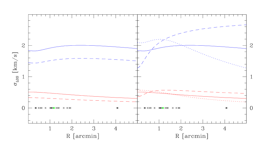
Figure 1.— Line-of-sight velocity dispersion profiles predicted by Newtonian (black lines; colored red in the online version) and MOND (grey lines; blue in the online version) models of Pal 14, assuming the cluster isolated. In the left panel isotropic models with different $M/L$ ratios ($M/L$=1.885: solid lines; $M/L$=0.747: dashed lines) are shown. In the right panel models with $M/L$=1.885 and different degrees of anisotropy (isotropic: solid lines; pure tangential: dashed lines; extremely radial: dotted lines) are shown. The radial locations of the target stars are marked at the bottom of both panels with black crosses. The thick cross (colored green in the online version) marks the location of star # 15.

Under the hypothesis that the cluster is isolated and spherically symmetric, simple models can be constructed by solving the Jeans equation

$$\frac{1}{\rho}\frac{d\sigma_{r}^{2}\rho}{dr}+2\beta\frac{\sigma_{r}^{2}}{r}=-\frac{d\Phi}{dr},$$ (2)

where $\rho$ is the density, $\Phi$ is the gravitational potential,

$$\beta(r)=1-\frac{\sigma_{t}^{2}(r)}{2\sigma_{r}^{2}(r)}$$ (3)

is the anisotropy parameter, and $\sigma_{r}$ and $\sigma_{t}$ are, respectively, the radial and tangential components of the velocity dispersion tensor at the radius $r$. If the system is self-gravitating, $\rho$ and $\Phi$ are related in Newtonian gravity by the Poisson equation

$$\nabla^{2}\Phi=4\pi G\rho,$$ (4)

while in MOND by the corresponding modified field equation (Bekenstein & Milgrom 1984)

$$\nabla\cdot\left[\mu\left(\frac{\|\nabla\Phi\|}{a_{0}}\right)\nabla\Phi\right]=4\pi G\rho,$$ (5)

where $\mu(x)$ is the so-called ”interpolating function” such that $\mu(x)\sim x$ at $x\ll 1$ (the so-called ”deep-MOND” regime) and $\mu(x)\sim 1$ at $x\gg 1$ (the Newtonian regime). In the following we use the ”simple” interpolating function $\mu(x)=x/(1+x)$ (Famaey & Binney 2005). For finite-mass isolated systems the boundary conditions of equations (4) and (5) are $|\nabla\Phi|\to 0$ for $|{\bf r}|\to\infty$, where ${\bf r}$ is the position vector.

For given density distribution and $\beta(r)$, equation (2) can be solved to obtain $\sigma_{r}$. The tangential component of the velocity dispersion $\sigma_{t}$ is then derived from eq. (3) and the line-of-sight (LOS) velocity dispersion at any given projected distance $R$ from the center is given by

$$\sigma_{LOS}^{2}(R)=\frac{2}{\Sigma(R)}\int_{R}^{{r_{t}}}\frac{{\rho}\left[\sigma_{r}^{2}\left({r}^{2}-R^{2}\right)+(\sigma_{t}^{2}/2)R^{2}\right]}{{r}\sqrt{{r}^{2}-R^{2}}}d{r}$$ (6)

where

$$\Sigma(R)=2\int_{R}^{{r_{t}}}\frac{{\rho}{r}}{\sqrt{{r}^{2}-R^{2}}}d{r}$$ (7)

is the projected density at $R$ and $r_{t}$ is the tidal radius. The above procedure allows to calculate a LOS velocity dispersion profile for any given choice of $M/L$ and $\beta(r)$ according to both Newtonian and MOND theories.

We adopted the density profile of the King (1966) model that best-fits the data of S11 defined by the parameters $(W_{0},r_{c},\mu_{V,0})=(7,0.61\arcmin,25.04~{}mag~{}arcsec^{-2})$ which have been converted in physical units assuming a distance of $d=71$ kpc and two different values of the mass-to-light ratio: $M/L_{V}$=1.885 (derived for Pal 14 from stellar population synthesis by McLaughlin & van der Marel 2005) and $M/L_{V}$=0.747 (corresponding to the minimum mass estimated by J09 from star counts in the color-magnitude diagram). Hereafter, we will refer to the M/L ratio in the V band simply as M/L. Regarding the degree of anisotropy, we considered, besides the isotropic case ($\beta=0$), two extreme anisotropic cases: purely tangential ($\beta=-\infty$) and maximally radial. In the latter case we adopted the Osipkov-Merritt parametrization (Osipkov 1979; Merritt 1985)

$$\beta({r})=\frac{{r}^{2}}{{r}^{2}+{r}_{a}^{2}},$$ (8)

where ${r}_{a}$ is the anisotropy radius, which sets the boundary where orbits become significantly radially biased (systems with smaller ${r}_{a}$ are more radially anisotropic). We assumed ${r}_{a}={r}_{a,min}$, where ${r}_{a,min}$ is the bona-fide minimum value for of ${r}_{a}$ for stability against radial-orbit instability. In particular, we adopt ${r}_{a,min}=2.8r_{c}$ for the Newtonian model and ${r}_{a,min}=3.1r_{c}$ for the MOND one, corresponding to the marginal condition for stability $2T_{r,half}/T_{t,half}\simeq 1.5$ (where $T_{r,half}$ and $T_{t,half}$ are the radial and tangential kinetic energies computed within the half-mass radius $r_{half}$; Nipoti et al. 2011; Ibata et al. 2011a).

The LOS velocity dispersion profiles of all these models, calculated by integrating numerically the above equations, are shown in Fig. 1. It is evident that, at least as long as the cluster is treated as isolated, MOND models predict a significantly larger velocity dispersion with respect to Newtonian ones (see also Baumgardt et al. 2005; Sollima & Nipoti 2010; Haghi et al. 2009, 2011). Newtonian and MOND velocity dispersion profiles are clearly distinct, regardless of the assumed anisotropy profile.

3.2. N-body simulations

As already reported above, all the models presented in the previous section are based on the assumption that the cluster is isolated. However, it is known that the presence of the Galactic field is important for Pal 14 (see Sect. 1), with different effects depending of the considered gravity law. In particular:

• In Newtonian gravity, the tidal interaction with the Galactic potential can alter the velocity dispersion of the system by heating stars at large distances from the center, by producing virial oscillations after tidal shocks and influencing its structural evolution;

• In MOND, besides the above tidal effects, even the presence of a uniform external field breaks the spherical symmetry of the gravitation field and can lead the cluster toward a less deep MOND regime (Bekenstein & Milgrom 1984).

To account properly for the above effects we used a set of N-body simulations performed in both Newtonian gravity and MOND. In the Newtonian case we studied the tidal effects by simulating the evolution of the cluster orbiting within the Galactic potential. In the MOND case we used N-body simulations to model the cluster in the presence of a uniform external field, so for simplicity we neglected the tidal effects. We note that, given the very long two-body relaxation time of Pal 14 ($t_{rh}\sim 19.9\,Gyr$; S11), its time evolution can be simulated also with collisionless N-body codes, which is especially convenient in MOND, because of the difficulty in realizing a collisional N-body code in this non-linear theory.

3.2.1 Newtonian simulations

Table 1Initial conditions of the Newtonian N-body simulations: orbital eccentricity ($e$), orbital energy ($E$), obital angular momentum ($L_{z}$), cluster mass (M), King (1966) central adimensional potential ($W_{0}$) and core radius ($r_{c}$).

Model	$e$	E	$L_{z}$	$P_{orb}$	M	$W_{0}$	$r_{c}$
#		($km/s^{2}$)	(km/s kpc)	(Gyr)	($M_{\odot}$)		(pc)
37/39	0.002	15962.05	9100	2.04	50000	9	12.6
41/43	0.5	5661.36	6300	2.23	380000	12	12.6
45/47	0.002	15962.05	9100	2.04	105000	12	12.6
49/51	0.5	5661.36	6300	2.23	170000	12	12.6

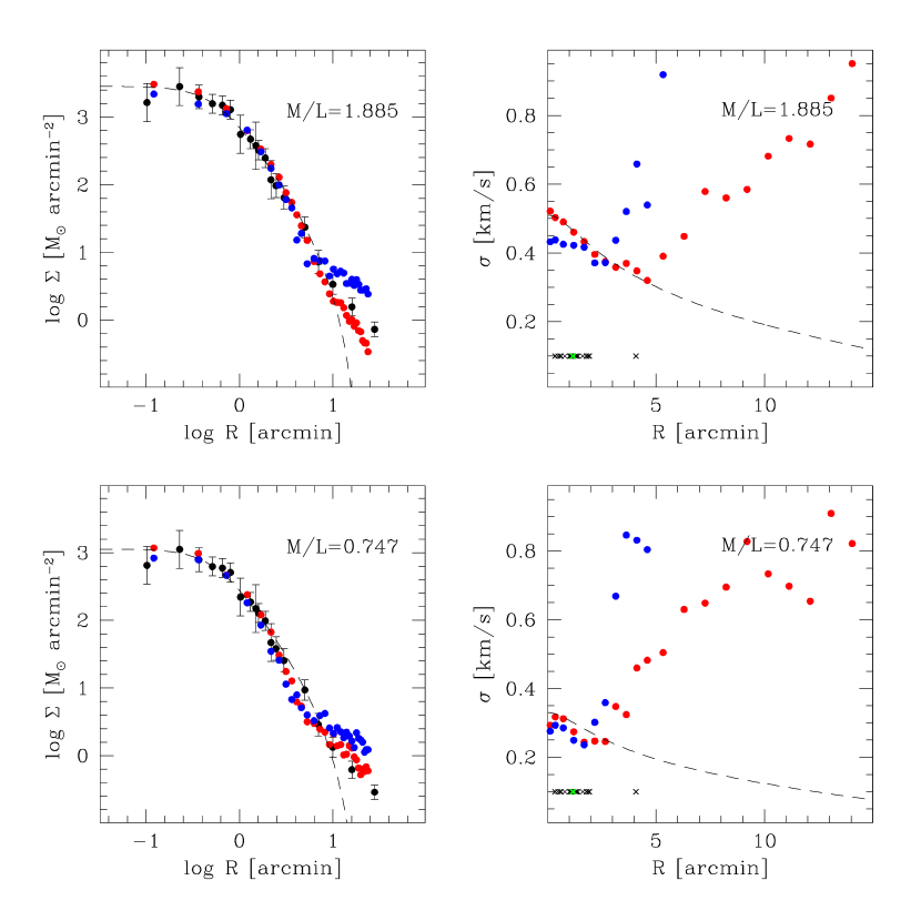
Figure 2.— Projected density profiles (left panels) and LOS velocity dispersion profiles (right panels) of the outcome of the N-body simulations performed in Newtonian dynamics assuming a quasi-circular orbit ($e=0.002$; red points) and an eccentric orbit ($e=0.5$; blue points). Upper panels refer to M/L=1.885, bottom panels to M/L=0.747. The density profile measures of S11 are marked with filled points with error bars in the left panels. The radial locations of the target stars are marked at the bottom of the right panel with black crosses, the green cross indicates the location of star #15. The predictions of the isolated Newtonian King (1966) model are also shown in all panels with dashed lines.

As already discussed in Sect. 3.2, the tidal interaction between Pal 14 and the Milky Way is expected to heat the outskirts of the cluster. This can be the result of both compressive shocks occurred during the disk crossing and perigalactic passages (Ostriker et al. 1972; Gnedin & Ostriker 1997) and the sudden change in the underlying potential (like in the case of the Sagittarius galaxy; Taylor & Babul 2001). After these episodes, the kinetic energy of a fraction of the cluster stars can exceed the boundaries of the cluster potential well and these stars become ”potential escapers” (Kupper et al. 2010). These stars might have a velocity dispersion larger than the other bound stars and remain within the cluster in spite of their positive energy for a timescale comparable to the cluster orbital period (Lee & Ostriker 1987). Moreover, the strong perturbations occurring after every disk passage affect the cluster virial equilibrium (and consequently its internal kinematics) producing damped oscillations which go on for many dynamical times (Gnedin & Ostriker 1999). Finally, the structural evolution of the cluster is also influenced by tides which accelerate the process of mass-loss (Gnedin et al. 1999). The overall effect on the cluster velocity dispersion is therefore extremely complex and not obviously resulting in a heating/freezing.

To evaluate the effect of tides on the velocity dispersion of Pal 14 we ran a set of N-body simulations. We used the last version of NBSymple (Capuzzo-Dolcetta et al. 2011), an efficient N-body integrator implemented on a hybrid CPU + GPU platform exploiting a double-parallelization on CPUs and on the hosted Graphic Processing Units (GPUs). The precision is guaranteed resorting to direct summation (to avoid truncation errors in force evaluation), and on the usage of high order, symplectic time integration methods (Kinoshita et al. 1991; Yoshida 1991). In particular the code allows to choose between two different symplectic integrators: a second order algorithm (commonly known as leapfrog) and a much more accurate (but also time consuming) sixth order method. The effect of the external galactic field is taken into account using an analytical representation of its gravitational potential. We adopted a leap-frog scheme with a time-step of $\Delta t=3.7\times 10^{4}~{}yr$ and a softening length of 0.2 pc (following the prescription of Dehnen & Read 2011). Such a relatively large time-step and softening length do not affect the accuracy of the simulation, because, as mentioned above, the effects of two-body encounters has been found to be negligible in this cluster even in its innermost region (S11; Beccari et al. 2011) and the relaxation times at the half-mass radius of our models are larger than the cluster age during the entire simulation. The cluster was launched within the three-component (bulge + disc + halo) static Galactic potential of Johnston et al. (1995) on two orbits with different eccentricities ($e\sim 0$ and $e=0.5$). First of all, we integrated backward in time, within the adopted potential, the orbit of a test particle from the apocenter (assumed to be the present-day location of the cluster at R=45.75 kpc, z=47.68 kpc, in cylindrical coordinates centered on the Galactic center) to the epoch $t=2~{}P_{orb}$ ago. At the end of the simulation, the model is within 40 pc of the current position of Pal 14 and the energy has been conserved within $\Delta E/E\sim 10^{-7}$ for both the considered orbits. Then the simulation has been launched with a cluster represented by 61,440 equal-mass particles distributed according to an equilibrium King (1966) model having initial mass, core radius and concentration empirically determined so that the projected density profile after two complete orbits reproduces the present-day cluster configuration (see Sect. 3.1). The initial conditions of the simulation for the two adopted orbits are reported in Table 1.

In Fig. 2 the final projected density and LOS velocity dispersion profiles are shown for the considered combinations of values of orbital eccentricity and M/L. It can be noted that in all cases the effect of tidal heating is visible only in the outermost radial bins of the projected density profiles, but a significant deviation from the predicted behavior of the isolated model is clearly visible in the velocity dispersion profiles beyond a distance from the cluster center which depends on the orbital eccentricity and the adopted M/L ratio. On the other hand, the isolated model remains a good representation of the cluster velocity dispersion at small distance from the cluster center, where most of the stars of the J09 sample reside.

3.2.2 MOND simulations

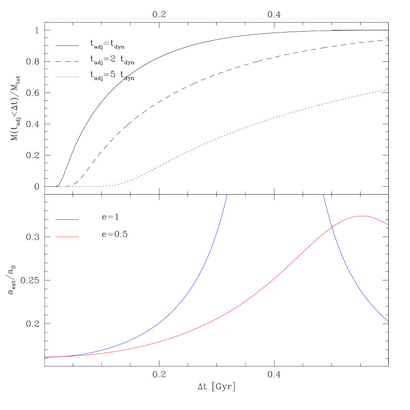
Figure 3.— Bottom panel: External acceleration exerted by the Milky Way on Pal 14 as a function of time elapsed from the present-day position (which is assumed to be the apocenter) for two different orbital eccentricities (e=1: grey line; e=0: black line; colored blue and red in the online version). Top panel: fraction of cluster stars with a timescale of adjustment with the external field ($t_{adj}$) shorter than the time elapsed from the initial position. The cases of $t_{adj}/t_{dyn}$=1, 2 and 5 are shown with solid, dashed and dotted lines, respectively. For instance in the case e=0.5, $\sim 0.56$ Gyr before the apocentric passage the modulus of the external field is twice the apocentric value (lower panel), but this time interval corresponds to more than 2 dynamical times for $\sim 90\%$ of the stars of the clusters (upper panel), which are thus likely to be now already in equilibrium with the current external field.

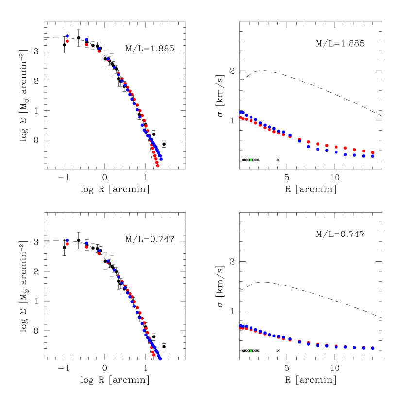
Figure 4.— Projected density profiles (left panels) and LOS velocity dispersion profiles (right panels) of the outcome of the $e=0$ (red points) and $e=0.5$ (blue points) MOND N-body simulations (see text for details). Upper panels refers to M/L=1.885, bottom panels to M/L=0.747. The density profile measures of S11 are marked with filled points with error bars in the left panel. The radial locations of the target stars are marked at the bottom of the right panel with black crosses, the green cross indicates the location of star #15. The corresponding isolated MOND models are represented in all panels with dashed lines.

The gravitational field of the Galaxy at the location of Pal 14 is estimated to be, in modulus, $g_{ext}\sim 0.16a_{0}$ (Johnston et al. 1995) and directed approximately towards the Galactic center. During its orbit the cluster will occupy different Galactic regions where the external field differs both in direction and in magnitude. The effect of such a variation on the internal kinematics of the cluster can be in principle significant (Kosowsky 2010) and is linked to the ratio between the timescale necessary to the cluster to reach a new equilibrium configuration ($t_{adj}$; which is of the order of the internal dynamical time $t_{dyn}$) and the orbital period ($P_{orb}$). Although the orbit of Pal 14 is unknown we can set an upper limit to this ratio by assuming the cluster presently at its apocenter and considering different orbital eccentricities. As a first order approximation, we calculated the orbital period assuming planar orbits within a spherical isothermal Galactic potential $\Phi_{MW}=v_{circ}^{2}\ln d_{GC}$ (where $d_{GC}$ is the Galactocentric distance) with $v_{circ}=198.9~{}km/s$, so $g_{ext}=0.16~{}a_{0}$ at $d_{GC}=66~{}kpc$ (the present-day Galactocentric distance of Pal 14). The dynamical time has been calculated as

$$t_{dyn}(r)=2\pi\sqrt{\frac{r}{d\Phi(r)/dr}}$$

adopting the cluster potential $\Phi(r)$ as in the isotropic MOND model of Pal 14 with $M/L$=1.885.

The ratio $t_{dyn}/P_{orb}$ is relatively small: even in the extreme case of a free falling orbit ($e=1$) we get $t_{dyn}/P_{orb}=0.23$ at the half-mass radius. To visualize the effect of the variation of the external acceleration on the internal cluster kinematics, we plot in Fig. 3 the external acceleration exerted on the cluster after a time interval $\Delta t$ from the current position (bottom panel) for two different eccentric orbits ($e=0.5$ and 1) and the fraction of mass comprised within the radius where $t_{adj}/t_{dyn}(r)=$1, 2 and 5. It is evident that assuming $t_{adj}/t_{dyn}$=1, more than 80% of the cluster stars reach the equilibrium with the external field within 100 Myr, a timescale during which the cluster feels an almost constant external acceleration (always smaller than $0.2~{}a_{0}$), regardless of its orbit. A more significant variation is instead noticeable assuming $t_{adj}$ of the order of few dynamical times: if $t_{adj}/t_{dyn}$=5 the external field doubles in the case of an orbit with eccentricity $e=0.5$ before $\sim 40\%$ of the cluster stars reached equilibrium, and the effect can be even more significant in the case of the free-falling orbit.

To evaluate the effect of the external field on the predicted velocity dispersion we used the MOND N-body code n-mody (Londrillo & Nipoti 2009), in which we implemented the external field effect as described in Ibata et al. (2011a). The presence of an uniform external field $-\nabla\Phi_{ext}$ is accounted for in the boundary conditions of equation (5), which become $\nabla\Phi\to\nabla\Phi_{ext}$ for $|{\bf r}|\to\infty$ (Bekenstein & Milgrom 1984). We recall that, due to technical difficulties, in MOND we do not simulate self-consistently the evolution of Pal 14 orbiting in the Galaxy (including tidal effects), but we limit ourselves to simple numerical experiments that should allow us to estimate reasonably well the effect of a uniform external field on the cluster velocity dispersion. In the simplest of our experiments we simulate the cluster in the presence of a uniform external field ${\bf g}_{ext}=-\nabla\Phi_{ext}$ that remains constant in modulus and direction throughout the simulation (see also Ibata et al. 2011a). In particular, in the attempt to model the cluster on a circular orbit, we fix $g_{ext}=0.16a_{0}$ (the value of the external field at the present-day location of Pal 14). In these simulations (which hereafter we refer to, loosely speaking, as $e=0$ MOND simulations) we let the cluster evolve for $\sim 2.3\,Gyr$ (i.e. slightly more than a complete orbital period).

If the cluster is on an eccentric orbit, not only the direction, but also the modulus of the external field varies during the orbit. In particular, if Pal 14 is currently at the apocenter it must have experienced a stronger external field in the past, which might affect to some degree its present-day velocity dispersion. In order to explore this effect, we also ran simulations in which the external field varies in time (in modulus, but not in direction) as expected for the $e=0.5$ orbit discussed above (see Fig. 3, bottom panel). In these simulations we follow the evolution of the cluster for $\sim 1.12\,Gyr$ (i.e. half orbit, starting at the apocenter): so, in this case the external field is $g_{ext}\simeq 0.16a_{0}$ at $t=0$ , it reaches a its maximum $g_{ext}\simeq 0.32a_{0}$ at $\sim 0.56\,Gyr$ and at the end of the simulation is again $g_{ext}\simeq 0.16a_{0}$ (loosely speaking hereafter we refer to these simulations as the $e=0.5$ MOND simulations).

For each value of $M/L$ ($M/L=0.747$ and $M/L=1.885$) we ran both the $e=0$ and the $e=0.5$ MOND simulations. In all cases, we initialized our N-body simulations with quasi-equilibrium distributions of $8\times 10^{5}$ particles: in practice we generate the initial conditions as follows. We first build an equilibrium Newtonian model with density given by the best-fitting King model of Pal 14 described in Section 3, and we then multiply the velocity of each particle by a factor $\left[\left(1+\tilde{g}_{ref}\right)/\tilde{g}_{ref}\right]^{1/2}$ (trying to reproduce the expected “quasi-Newtonian” behavior), where $\tilde{g}_{ref}\equiv g_{ref}/a_{0}$, and $g_{ref}$ is a reference gravitational field modulus. The value of $g_{ref}$ is empirically chosen in each case in order to have at the end of the simulation a mock cluster with a surface-density profile consistent with the observed profile of Pal 14. In the case of the $e=0$ simulations $g_{ref}=g_{ext}=0.16a_{0}$; in the case of the $e=0.5$ simulations $g_{ref}=\langle{g_{ext}}\rangle=0.22a_{0}$, where $\langle{g_{ext}}\rangle$ is the time-averaged modulus of the external field for the considered orbit.

In the $e=0$ simulations the system readjusts itself in a few dynamical times into a new equilibrium configuration. In the $e=0.5$ simulations the cluster is continuously slowly evolving due to the variation of the external field. In both cases the end-products of the simulations are axisymmetric configurations with symmetry axis along the direction of the external field. When projected along the line-of-sight to Pal 14 (assuming that the field of the Galaxy points toward the Galactic center) the systems appear almost circular (with ellipticity $\epsilon\sim 0.01$) and with circularized surface-density distribution very similar to the observed light distribution of Pal 14 (see Fig. 4, left panels). In Fig. 4 we also show the velocity dispersion profiles of the end-products of the $e=0$ and $e=0.5$ MOND simulations (right panels). It is apparent that when the external field is taken into account the velocity dispersion profile is at all radii significantly lower than that of the corresponding isolated model. As we will see in Sect. 5.1, this effect is crucial in the comparison between the MOND predictions and the data, in particular when low values of $M/L$ are assumed. On the other hand, the orbital eccentricity does not affect significantly the velocity dispersion profile, indicating that the cluster quickly reaches the equilibrium with the external field at the apocenter and does not keep memory of the stronger external field experienced in the past.

3.3. Binary population

It is well known that a significant population of undetected binaries can inflate the measured velocity dispersion (Blecha et al. 2004), because in a binary system the relative projected velocity of the primary component is added to the motion of the center of mass, introducing an additional spread in the velocity distribution of the whole population. To account for the effect of a binary population on the velocity dispersion, we constructed a library of binaries which has been used in the Monte Carlo procedure.

Following McConnachie & Cote (2010) the projected velocity of the primary component in a binary system is given by

$$v=\frac{2\pi a_{1}\sin i}{P(1-e^{2})^{1/2}}[\cos(\theta+\omega)+e\cos\omega],$$

where $m_{1}$ and $m_{2}$ are the masses of the primary and secondary component, $a_{1}$ is the semi-major axis of the primary component, $P$ is the orbital period, $e$ the eccentricity, $i$ the inclination angle to the line-of-sight, $\theta$ the phase from the periastron and $\omega$ the longitude of the periastron. For each simulated binary we extracted randomly a combination of ($m_{1},m_{2},P,e,\theta,\omega,i$) from suitable distributions and derived the corresponding projected velocity $v$.

We randomly extracted a large number ($N>10^{6}$) of stars from the IMF of Kroupa (2002) with masses $0.08<M/M_{\odot}<7$ and paired them imposing that the distribution of mass ratios in the primary component mass range $1<m_{1}/M_{\odot}<7$ must be equal to that measured by Fisher et al. (2005) in the solar neighborhood. To do this, an iterative algorithm has been used: at every iteration stars are paired randomly and a ”chance of pairing” as a function of the mass ratio has been computed as the ratio between the output mass ratio normalized distribution calculated in the above primary component mass range and that of Fisher et al. (2005). Then, a subsample of binaries has been extracted according to the chance of pairing associated to their mass ratio and added to the library, while the components of the rejected binaries are used as input in the next iteration until all stars are paired. Then, we selected from the library all binaries whose primary component is within $|m_{1}-M_{RGB}|<0.05M_{\odot}$, where $M_{RGB}=0.83~{}M_{\odot}$ is the typical mass of a RGB star calculated by comparing the color-magnitude diagram of Pal 14 of S11 with a suitable isochrone of Marigo et al. (2008). We followed the prescriptions of Duquennoy & Mayor (1991) for the distribution of periods and eccentricities. The semi-major axis has been calculated using the third Kepler law

$$a_{1}=\frac{1}{1+\frac{m_{1}}{m_{2}}}\left[\frac{P^{2}G(m_{1}+m_{2})}{4\pi^{2}}\right]^{1/3}.$$

We removed all those binaries whose corresponding semi-major axes lie outside the range $a_{min}<a<100$ AU where $a_{min}$ is linked to the radius of the secondary component (according to Lee & Nelson 1988). The distribution of the angles ($i,\theta,\omega$) has been chosen according to the corresponding probability distributions (${\rm Prob}(i)\propto\sin~{}i;~{}{\rm Prob}(\theta)\propto\dot{\theta}^{-1};~{}{\rm Prob}(\omega)={\rm constant}$).

For a given fraction of binaries $f_{b}$ the effective fraction $f_{b}^{RGB}$ is calculated as the ratio between the number of binaries with $|m_{1}-M_{RGB}|<0.05M_{\odot}$ ($N_{b,RGB}$) and the number of objects (singles+binaries) in the same mass range ($N_{s,RGB}+N_{b,RGB}$) as

$$f_{b}^{RGB}=\frac{f_{b}N_{b,RGB}}{(1-f_{b})N_{s,RGB}\frac{N_{b,tot}}{N_{s,tot}}+f_{b}N_{b,RGB}}.$$

Note that in our Monte Carlo simulations we assumed that the binary population has the same radial distribution as single stars. This assumption is justified by the observed lack of mass segregation observed in this cluster (Beccari et al. 2011).

4. Monte Carlo simulations

Table 2Summary of the Monte Carlo simulations. The table lists the model ID, the adopted theory of gravity, the kind of anisotropy, the M/L ratio, the cluster orbital eccentricity ($e$), the binary fraction ($f_{b}$), the rejection threshold and the derived velocity dispersion quantiles 50% (median), 16% and 84% ($\sim~{}1\sigma$)

Model	Gravity	anisotropy	M/L	$e$	$f_{b}$	rejection threshold	$\sigma_{v}$
#			$M_{\odot}/L_{V,\odot}$		%	$\sigma$	f(16%)	f(50%)	f(84%)
1	Newtonian	isotropic	1.885	isolated	0	3	0.30	0.42	0.56
2	MOND	isotropic	1.885	isolated	0	3	1.52	1.84	2.27
3	Newtonian	isotropic	1.885	isolated	0	5	0.32	0.41	0.58
4	MOND	isotropic	1.885	isolated	0	5	1.45	1.90	2.19
5	Newtonian	isotropic	0.747	isolated	0	3	0.16	0.27	0.41
6	MOND	isotropic	0.747	isolated	0	3	1.25	1.48	1.90
7	Newtonian	isotropic	0.747	isolated	0	5	0.15	0.29	0.40
8	MOND	isotropic	0.747	isolated	0	5	1.19	1.50	1.80
9	Newtonian	tangential	1.885	isolated	0	3	0.38	0.48	0.67
10	MOND	tangential	1.885	isolated	0	3	1.59	2.06	2.33
11	Newtonian	tangential	1.885	isolated	0	5	0.39	0.49	0.68
12	MOND	tangential	1.885	isolated	0	5	1.72	1.97	2.47
13	Newtonian	radial	1.885	isolated	0	3	0.31	0.47	0.59
14	MOND	radial	1.885	isolated	0	3	1.60	2.04	2.41
15	Newtonian	radial	1.885	isolated	0	5	0.32	0.45	0.59
16	MOND	radial	1.885	isolated	0	5	1.56	1.95	2.37
17	Newtonian	isotropic	1.885	isolated	10	3	0.26	0.49	0.68
18	Newtonian	isotropic	1.885	isolated	10	5	0.32	0.51	0.91
19	Newtonian	isotropic	0.747	isolated	10	3	0.13	0.31	0.50
20	Newtonian	isotropic	0.747	isolated	10	5	0.16	0.32	0.77
21	Newtonian	isotropic	1.885	isolated	20	3	0.27	0.57	0.94
22	Newtonian	isotropic	1.885	isolated	20	5	0.42	0.77	1.20
23	Newtonian	isotropic	0.747	isolated	20	3	0.01	0.34	0.61
24	Newtonian	isotropic	0.747	isolated	20	5	0.24	0.59	1.09
25	Newtonian	isotropic	1.885	isolated	30	3	0.36	0.71	1.33
26	Newtonian	isotropic	1.885	isolated	30	5	0.65	1.00	1.47
27	Newtonian	isotropic	0.747	isolated	30	3	0.15	0.56	1.12
28	Newtonian	isotropic	0.747	isolated	30	5	0.48	0.92	1.39
29	Newtonian	isotropic	1.885	isolated	40	3	0.61	1.15	1.70
30	Newtonian	isotropic	1.885	isolated	40	5	0.84	1.17	1.74
31	Newtonian	isotropic	0.747	isolated	40	3	0.31	0.66	1.41
32	Newtonian	isotropic	0.747	isolated	40	5	0.74	1.14	1.71
33	Newtonian	isotropic	1.885	isolated	50	3	0.98	1.43	2.05
34	Newtonian	isotropic	1.885	isolated	50	5	1.04	1.52	1.93
35	Newtonian	isotropic	0.747	isolated	50	3	0.59	1.31	1.77
36	Newtonian	isotropic	0.747	isolated	50	5	0.77	1.31	1.69
37	Newtonian	isotropic	1.885	0.002	0	3	0.31	0.42	0.59
38	MOND	isotropic	1.885	0	0	3	0.80	0.95	1.23
39	Newtonian	isotropic	1.885	0.002	0	5	0.32	0.46	0.58
40	MOND	isotropic	1.885	0	0	5	0.76	0.97	1.20
41	Newtonian	isotropic	1.885	0.5	0	3	0.30	0.42	0.57
42	MOND	isotropic	1.885	0.5	0	3	0.61	0.81	1.14
43	Newtonian	isotropic	1.885	0.5	0	5	0.29	0.39	0.57
44	MOND	isotropic	1.885	0.5	0	5	0.60	0.83	1.13
45	Newtonian	isotropic	0.747	0.002	0	3	0.14	0.27	0.37
46	MOND	isotropic	0.747	0	0	3	0.45	0.59	0.76
47	Newtonian	isotropic	0.747	0.002	0	5	0.15	0.28	0.38
48	MOND	isotropic	0.747	0	0	5	0.48	0.59	0.78
49	Newtonian	isotropic	0.747	0.5	0	3	0.11	0.25	0.41
50	MOND	isotropic	0.747	0.5	0	3	0.32	0.54	0.71
51	Newtonian	isotropic	0.747	0.5	0	5	0.01	0.29	0.36
52	MOND	isotropic	0.747	0.5	0	5	0.33	0.51	0.72

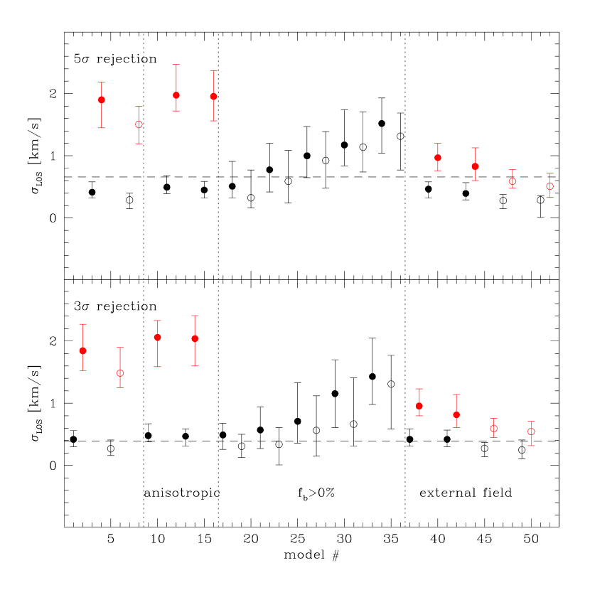
Figure 5.— Projected velocity dispersion and range comprising 68% of realizations predicted by the whole set of Monte Carlo simulations. Black dots mark the prediction of Newtonian models, grey dots (red in the online version) the predictions of MOND models. Filled symbols refer to M/L=1.885, open symbols refer to M/L=0.747.

To compare the velocity dispersion measured in Sect. 2 with the models described in Sect. 3 we adopted a Monte Carlo approach. In particular, we first defined a rejection criterion and selected a subsample of member stars from the J09 radial velocities accordingly. Here, we adopted a preliminary exclusion of all stars with $|v-\overline{v}|>5~{}km/s$, and a subsequent $\sigma$ clipping rejection. We considered the cases of a 3$\sigma$ and a 5$\sigma$ threshold—where $\sigma\equiv\sqrt{\sigma_{v}^{2}+\delta_{i}^{2}+\delta(\overline{v})^{2}}$ includes the intrinsic velocity dispersion $\sigma_{v}$, the individual error $\delta_{i}$ and the error on the mean $\delta(\overline{v})$—which define two samples with $N=16$ and $N=17$ stars (including star #15), respectively. Then, once selected a model and a binary fraction $f_{b}$, for each star of the observed sample the following steps have been performed:

1. We compute the distance of the star from the cluster center $R_{i}$ and extract a velocity corresponding to the local LOS velocity dispersion in the model. The extraction algorithm depends on the kind of model:

   • for the analytical models, the velocity is randomly extracted from a Gaussian distribution with dispersion $\sigma_{LOS}(R_{i})$ i.e. the projected velocity dispersion at the star distance from the center;

   • for the N-body models, the velocity is extracted from the last snapshot of the N-body simulation: for each star a random position angle is extracted and the projected velocity of the closest particle in the N-body system is adopted.

2. We extract a random velocity from a Gaussian distribution with dispersion $\delta_{i}$ and sum it to the previous one to compute a simulated observational velocity;

3. A random number between 0 and 1 is extracted from a uniform distribution. If such number is smaller than the effective binary fraction $f_{b}^{RGB}$ (see Sect. 3.3) a binary is randomly extracted from the library defined in Sect. 3.3 and its apparent velocity is added to the simulated velocity.

Then the rejection criterion is applied to the simulated sample and for every rejected velocity another extraction is made at the same location. In this way, every realization is constituted by the same number of object at the same location as the observed sample. Finally, the velocity dispersion of the simulated sample is calculated using eq. 1. The above procedure is repeated 1000 times to compute the distribution of predicted velocity dispersions. The outcome of all the performed simulations is summarized in Table 2 and illustrated in Fig. 5.

5. Results

5.1. Newtonian vs. MOND models

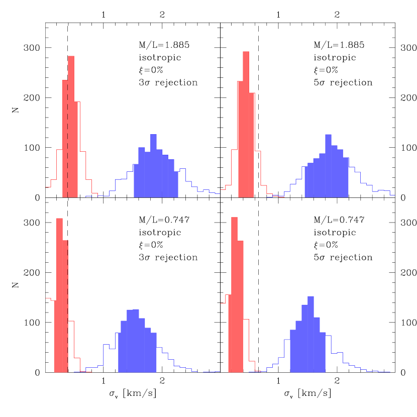
Figure 6.— Distribution of predicted velocity dispersions for Newtonian (red histograms) and MOND (blue histograms) isolated isotropic models with $f_{b}=0$ and $M/L$=1.885 (upper panels) and $M/L$=0.747 (bottom panels). Left panels refer to the 3$\sigma$ rejection threshold, right panels to the 5$\sigma$ rejection threshold. Shaded areas indicate the range (centered on the median) comprising 68% of realizations. The observed velocity dispersions are also marked in all panels with dashed lines.

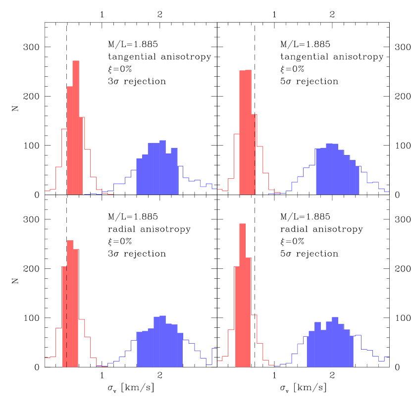
Figure 7.— Same as Fig. 6, but for models purely tangential (upper panels) and extremely radial (bottom panels) anisotropy (assuming $M/L$=1.885).

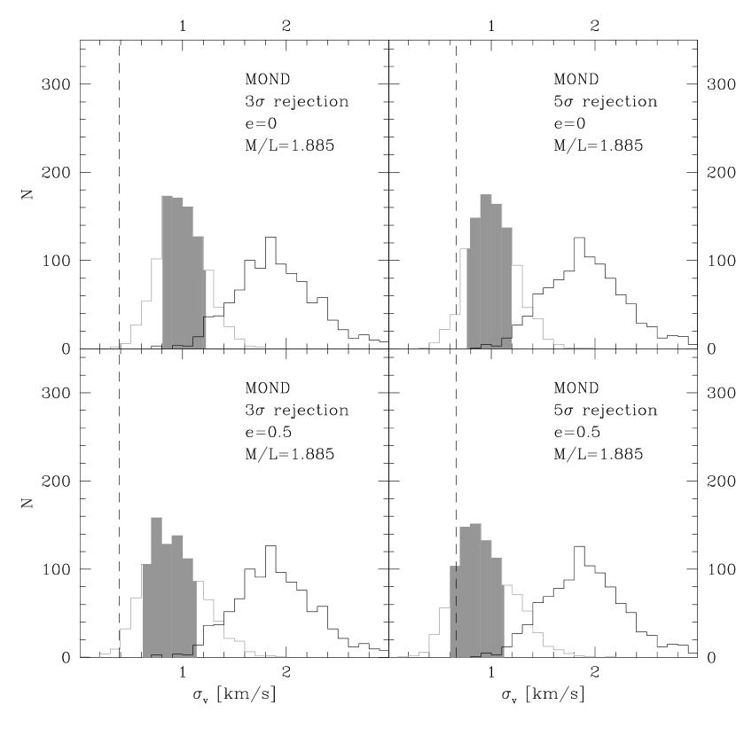
Figure 8.— Distribution of predicted velocity dispersions for isolated isotropic MOND models with $M/L$=1.885 and $f_{b}=0$ (black histograms) and models immersed in the external Galactic field (grey histograms), assuming a circular orbit (upper panels) and an eccentric orbit with e=0.5 (lower panels). Left panels refer to the 3$\sigma$ rejection threshold, right panels to the 5$\sigma$ rejection threshold. Shaded areas indicate the range (centered on the median) comprising 68% of realizations. The observed velocity dispersions are marked in all panels with dashed lines.

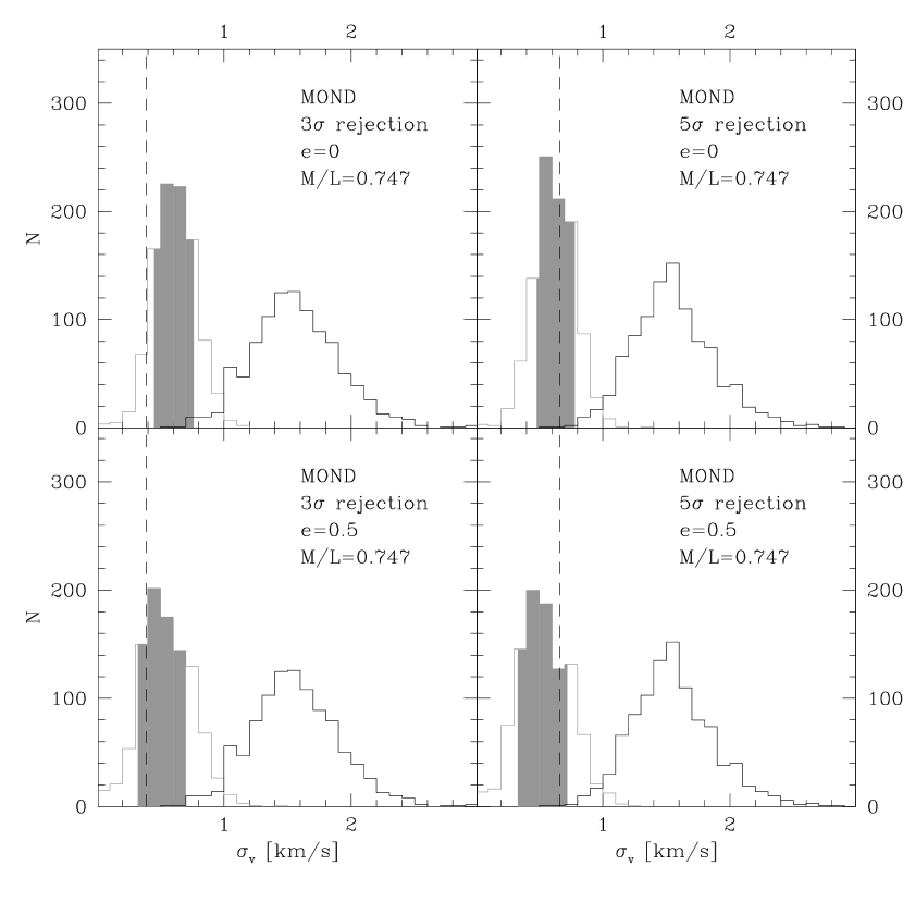
Figure 9.— Same as Fig. 8, but for models with $M/L$=0.747.

In Figs. 6 and 7 the distributions of predicted velocity dispersions are shown for isolated models with no binaries and different values of $M/L$ and degrees of anisotropy, respectively. It is apparent that while Newtonian models with M/L=1.885 predict velocity dispersions which are compatible with the observed value, Newtonian models with a M/L=0.747 tend to underpredict the systemic velocity dispersion, while all extractions from isolated MOND models predict velocity dispersions larger than the observed (even when $M/L$ is as low as 0.747). It is interesting to note that anisotropy has only a small effect on the predicted distribution of velocity dispersions. This is because most of the J09 sample is constituted by stars located between $1\arcmin<R<2\arcmin$, a region where all the models predict a similar velocity dispersion regardless of the degree of anisotropy (see Fig. 1).

In Fig. 8 and 9 the distributions of velocity dispersions predicted by MOND models including the external field effect (for the considered orbits and M/L ratios) are compared with that of the isolated MOND model. As anticipated in Sect. 3.2.2, it is apparent that the inclusion of the external field significantly affects the predicted velocity dispersion reducing the systemic velocity dispersion. For a $M/L$=1.885 (the one predicted by stellar evolution models for Pal 14), it is clear that the predicted velocity dispersion, though significantly influenced by the external field, remains in any case higher than the observed value (Fig. 8). A small, but not negligible ($\sim 20$%), number of realizations compatible with observations are noticeable when a stronger external field and a 5$\sigma$ rejection threshold are considered. Note that a non-zero binary fraction and the tidal heating (not included in these simulations) could inflate the model velocity dispersion making the discrepancy between the MOND predictions and the data even larger. Instead, for a lower $M/L$=0.747 ratio the predictions of MOND models agree with the measured velocity dispersion (see Fig. 9). So we conclude that the adoption of a low $M/L$ ratio, in association with the adoption of a 5$\sigma$ rejection criterion and/or a large orbital eccentricity, could reconcile MOND with the observed properties of Pal 14.

5.2. Binary fraction

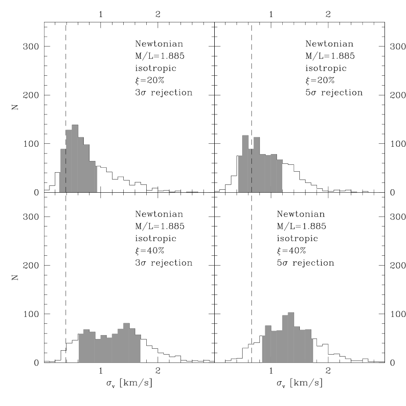
Figure 10.— Distribution of predicted velocity dispersions for isotropic Newtonian models with $f_{b}=20\%$ (upper panels) and $f_{b}=40\%$ (bottom panels), assuming $M/L$=1.885. Left panels refer to the 3$\sigma$ rejection threshold, right panels to the 5$\sigma$ rejection threshold. Grey areas indicate the range (centered on the median) comprising 68% of realizations. The observed velocity dispersions are marked in all panels with dashed lines.

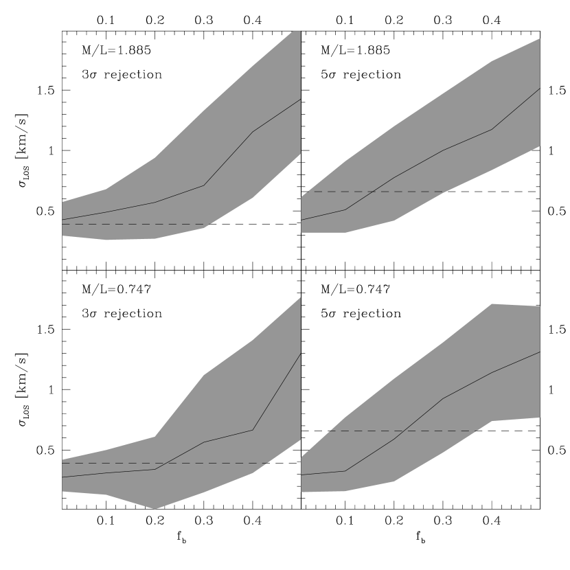
Figure 11.— Median (solid line) and range including 68% of realizations (grey shaded area) for isotropic Newtonian models with $M/L$=1.885 as functions of the adopted binary fraction. Left panels refer to the 3$\sigma$ rejection threshold, right panels to the 5$\sigma$ rejection threshold. Upper panels refers to M/L=1.885, bottom panels to M/L=0.747. The observed velocity dispersions are marked in all panels with dashed lines.

In Fig. 10 the distributions of predicted velocity dispersions are shown for (isolated) isotropic Newtonian models with $M/L$=1.885 and two different binary fractions ($f_{b}=20\%$ and $f_{b}=40\%$). As expected, as the fraction of binaries increases the distribution appears to be shifted to higher velocity dispersions. In Fig. 11 the median of the distribution and the range including 68% of realizations are plotted as functions of the adopted binary fraction for the two considered M/L ratios. From the comparison with the observed velocity dispersion of the sample of J09 we conclude that models with $f_{b}<30\%$ in the case of M/L=1.885, and slightly larger $f_{b}<40\%$ for M/L=0.747 are still acceptable.

These upper limits are larger than that derived by Kupper & Kroupa (2010; $f_{b}\leq 10\%$). There are three noticeable differences between the analysis presented here and that performed by these authors: i) they adopt a different rejection criterion which rejects stars outside a fixed velocity window, ii) they adopt different characteristics for their binary population and iii) they compute the velocity dispersion from subsamples of stars selected randomly across the cluster. We note that while the first two choices are somewhat arbitrary, the latter represents a limitation of Kupper & Kroupa (2010) analysis. Such difference can well be responsible for the higher predicted velocity dispersion and the corresponding smaller limit to the cluster binary fraction found by Kupper & Kroupa (2010).

5.3. The effect of tidal heating in the J09 sample

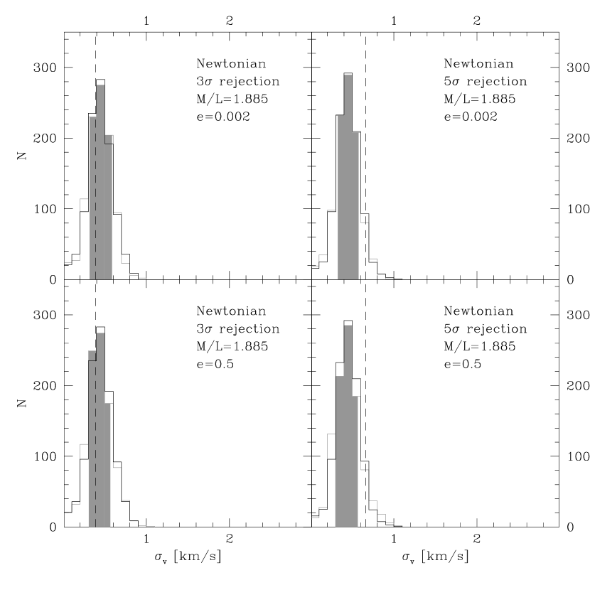
Figure 12.— Distribution of predicted velocity dispersions for isolated isotropic Newtonian models with $M/L$=1.885 and $f_{b}=0$ (black histograms) and models immersed in the external Galactic tidal field (grey histograms). In the upper and bottom panels models on quasi-circular orbits ($e=0.002$) and on eccentric ($e=0.5$) orbits are considered, respectively. Left panels refer to the 3$\sigma$ rejection threshold, right panels to the 5$\sigma$ rejection threshold. Shaded areas indicate the range (centered on the median) comprising 68% of realizations. The observed velocity dispersions are marked in all panels with dashed lines.

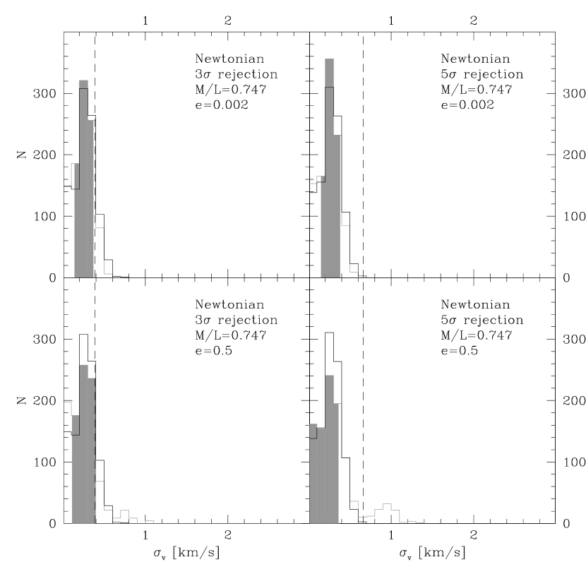
Figure 13.— Same as Fig. 12, but for models with $M/L$=0.747.

The N-body simulations described in Sect. 3.2.1 allow to evaluate the effect that tides have in the stellar kinematics of Pal 14 in the framework of the classical Newtonian dynamics. Quantifying this effect is important since it can potentially affect the cluster velocity dispersion measured through the J09 sample (Kupper et al. 2010).

The output distributions of predicted velocity dispersions for the two orbits are compared to the isolated model in Fig. 12 and Fig. 13 for M/L=1.885 and M/L=0.747, respectively. It is apparent that the effect of tidal heating is negligible in all cases. A small difference is noticeable only in the M/L=0.747 case when eccentric orbits are considered: in this case the distribution, while having the same peak value, present a larger dispersion and a tail extending toward larger velocity dispersions. The reason of this result can be found by looking at the spatial distribution of the J09 sample: 16 out 17 target stars reside in the inner 2 arcminutes, a region where tides have only a minor heating efficiency (see Fig. 2). The effect is indeed slightly more evident when a small M/L and an eccentric orbit are considered, since the effect of heating penetrates deeper into the cluster affecting the velocity of the two outermost targets. We conclude that the upper limit in the binary fraction derived in Sect. 5.2 is not altered by this effect, at least for the two considered orbits.

6. Discussion

Using a Monte Carlo approach, we performed an accurate comparison of the velocity dispersion of the globular cluster Pal 14 measured from high-resolution radial velocities with the predictions of a set of dynamical models spanning a wide range in $M/L$ ratio, degree of anisotropy, binary fraction and orbital eccentricity in both Newtonian and MOND gravity. The obtained results indicate that Newtonian models with a binary fraction $f_{b}<30\%$ and a $M/L$ ratio compatible with the predictions of stellar evolutionary models are in good agreement with the kinematics of this stellar system. On the other hand MOND models with the same $M/L$ ratio appear to systematically overpredict the velocity dispersion for any assumption of the cluster anisotropy. The same conclusion has been reached previously by J09 but questioned by Gentile et al. (2010). Note that all these previous approaches compared the velocity dispersion with the prediction of theoretical models neglecting the information on the radial distribution of targets. This has an important impact in increasing the significance of the comparison as most of targets are actually located in the central part of the cluster where the difference between Newtonian and MOND models is maximized. Moreover, our simulations showed the importance of the inclusion of the external field in the determining the velocity dispersion profile of MOND models for this cluster. This warns against using isolated MOND models for clusters with masses and Galactocentric distances similar to Pal 14 (see also Baumgardt et al. 2005, Haghi et al. 2009, 2011). Similar difficulties for MOND in explaining the internal kinematics of GCs have been already found in previous studies on NGC2419 (Baumgardt et al. 2009; Sollima & Nipoti 2010; Ibata et al. 2011a,b). In this last case the effect of the external field, which is a factor 1.4 weaker in modulus and $\sim$23 times smaller with respect to the cluster internal acceleration than in Pal 14, has been estimated to be negligible (Ibata et al. 2011a).

The conclusions are different when significantly lower values of $M/L$ are considered for Pal 14. In this case the predictions of MOND models are close the observed velocity dispersion (in particular when a 5$\sigma$ rejection criterion is adopted and eccentric orbits are considered), while Newtonian models predict a lower velocity dispersion. So, a combination of small $M/L$ ratio, small binary fraction, relatively large orbital eccentricity and the adoption of a permissive rejection criterion provides a way-out for MOND. As the $M/L$ ratio is a crucial parameter in the presented analysis, it is interesting to discuss in more detail the possibility of constraining its value.

From a theoretical point of view, the M/L ratio of an old, metal-poor stellar population composed mainly by subsolar-mass stars is expected to be systematically larger than unity ($1.5<M/L<2.5$; Fioc & Rocca-Volmerange 1997; Bruzual & Charlot 2003) and can reach $M/L>3$ if dark remnants are taken into account (Kruijssen 2009). On the other hand, observational analyses performed on GCs in the Milky Way and M31 have shown the occurrence of a sparse number of clusters with M/L values as small as M/L$\sim$0.6 (Strader et al. 2009, 2011). It is worth noting that the low M/L=0.747 ratio adopted here corresponds to the minimum mass calculated by J09 assuming a decreasing mass function for stellar masses smaller than the limiting magnitude of deep photometric HST observations of Pal 14 and neglecting the effect of dark remnants. So $M/L=0.747$ must be considered a strong lower limit. On the other hand, while the value of M/L=1.885 derived by McLaughlin & van der Marel (2005) assumes a standard Chabrier (2003) IMF, J09 measured a shallower mass function slope in the limited mass range covered by their observations which could in turn suggest a lower M/L as appropriate. In general, the dynamical M/L ratios measured in GCs appear generally smaller than those predicted by population synthesis models ($(M/L)_{dyn}/(M/L)_{syn}=0.82\pm 0.07$ with some cluster with even smaller values; McLaughlin & van der Marel 2005). Furthermore, in stellar systems with a small binding energy like Pal 14, the recoil speed of white dwarf remnants could exceed the cluster escape velocity, causing a substantial loss of dark remnants (Fellhauer et al. 2003). Primordial mass segregation can also play a role favoring the losses of low-mass stars (with high individual M/L ratio; Zoonozi et al. 2011). Therefore, mass-to-light ratios substantially lower than that predicted by stellar evolution models cannot be excluded. A very low binary fraction also appears disfavored (see below), although direct estimates of the binary fraction in this cluster are still missing.

The comparison between the observed velocity dispersion and the Newtonian predictions sets an upper limit for the fraction of binaries in this cluster $f_{b}<30\%$ ($f_{b}<40\%$ for the case of low M/L=0.747), significantly higher than the upper limit ($f_{b}<10\%$) estimated by Kupper & Kroupa (2010; see the discussion in Section 5.2). These upper limits must be compared with independent estimates of the binary fraction of Pal 14. Unfortunately, the deepest photometric studies on this cluster (Dotter et al. 2008) barely reach $\sim 3$ magnitudes below the cluster turn-off, therefore preventing any direct estimate of the binary fraction. However, an indirect estimate of the binary content of Pal 14 $f_{b}\sim 30-40\%$ has been recently provided by Beccari et al. (2011) on the basis of the comparison between the fraction of Blue Straggler Stars and binary fraction in clusters with similar mass and density. So, on the basis of the above estimate we conclude that the observed velocity dispersion of this cluster is consistent with the Newtonian theory of gravity. Also in this case, this result has been validated only for orbits with eccentricities $e<0.5$. Orbits with a larger eccentricity can in principle lead to a significant heating of the cluster also in its innermost region, where most of the J09 targets are located. However, we suggest that the available data do not provide any significant indication of a failure of the Newtonian theory of gravity.

The present analysis can also be used to gain insight into the question of the dark matter content of Pal 14: in the framework of the classical Newtonian dynamics the low observed velocity dispersion implies a dynamical $M/L\leq 1.5-2$ (for reasonable assumptions on the binary fraction and on the rejection criterion). This result, combined with the observation that Pal 14 has significant tidal tails (S11), suggests that dark matter does not contribute substantially to the mass of this remote GC.

References

- Baumgardt et al. (2005) Baumgardt, H., Grebel, E. K., & Kroupa, P. 2005, MNRAS, 359, L1
- Baumgardt et al. (2009) Baumgardt, H., Côté, P., Hilker, M., Rejkuba, M., Mieske, S., Djorgovski, S. G., & Stetson, P. 2009, MNRAS, 396, 2051
- Beccari et al. (2011) Beccari, G., Sollima, A., Ferraro, F.R., Lanzoni, B., Bellazzini, M., De Marchi, M. 2011, ApJ, 737, 3
- Bekenstein & Milgrom (1984) Bekenstein, J.D., & Milgrom, M. 1984, ApJ, 286, 7
- Blecha et al. (2004) Blecha, A., Meylan, G., North, P., & Royer, F. 2004, A&A, 419, 533
- Bruzual & Charlot (2003) Bruzual, G., & Charlot, S. 2003, MNRAS, 344, 1000
- Capuzzo-Dolcetta et al. (2011) Capuzzo-Dolcetta, R., Mastrobuono-Battisti, A., & Maschietti, D. 2011, New Astronomy, 16, 284
- Chabrier (2003) Chabrier, G. 2003, ApJ, 586, L133
- Dehnen & Read (2011) Dehnen, W., & Read, J. I. 2011, European Physical Journal Plus, 126, 55
- Dotter et al. (2008) Dotter, A., Sarajedini, A., & Yang, S.-C. 2008, AJ, 136, 1407
- Duquennoy & Mayor (1991) Duquennoy, A., & Mayor, M. 1991, A&A, 248, 485
- Famaey & Binney (2005) Famaey, B., & Binney, J. 2005, MNRAS, 363, 603
- Fellhauer et al. (2003) Fellhauer, M., Lin, D. N. C., Bolte, M., Aarseth, S. J., & Williams, K. A. 2003, ApJ, 595, L53
- Fioc & Rocca-Volmerange (1997) Fioc, M., & Rocca-Volmerange, B. 1997, A&A, 326, 950
- Fisher et al. (2005) Fisher, J., Schröder, K.-P., & Smith, R. C. 2005, MNRAS, 361, 495
- Gentile et al. (2010) Gentile, G., Famaey, B., Angus, G., & Kroupa, P. 2010, A&A, 509, A97
- Gnedin & Ostriker (1999) Gnedin, O. Y., & Ostriker, J. P. 1999, ApJ, 513, 626
- Gnedin et al. (1999) Gnedin, O. Y., Lee, H. M., & Ostriker, J. P. 1999, ApJ, 522, 935
- Gnedin & Ostriker (1997) Gnedin, O. Y., & Ostriker, J. P. 1997, ApJ, 474, 223
- Haghi et al. (2009) Haghi, H., Baumgardt, H., Kroupa, P., Grebel, E. K., Hilker, M., & Jordi, K. 2009, MNRAS, 395, 1549
- Haghi et al. (2011) Haghi, H., Baumgardt, H., & Kroupa, P. 2011, A&A, 527, A33
- Ibata et al. (2011a) Ibata, R., Sollima, A., Nipoti, C., Bellazzini, M., Chapman, S.C., Dalessandro, E. 2011a, ApJ, 738, 186
- Ibata et al. (2011b) Ibata, R., Sollima, A., Nipoti, C., Bellazzini, M., Chapman, S.C., Dalessandro, E. 2011b, ApJ, in press (arXiv:1110.3892)
- Johnston et al. (1995) Johnston, K. V., Spergel, D. N., & Hernquist, L. 1995, ApJ, 451, 598
- Johnston et al. (1999) Johnston, K. V., Sigurdsson, S., & Hernquist, L. 1999, MNRAS, 302, 771
- Jordi et al. (2009) Jordi, K., et al. 2009, AJ, 137, 4586
- King (1966) King, I. R. 1966, AJ, 71, 64
- Kinoshita et al. (1991) Kinoshita, H., Yoshida, H., & Nakai, H. 1991, Celestial Mechanics and Dynamical Astronomy, 50, 59
- Kosowsky (2010) Kosowsky, A. 2010, Advances in Astronomy, 2010, arXiv:0910.4802
- Kroupa (1995) Kroupa, P. 1995, MNRAS, 277, 1491
- Kroupa (2002) Kroupa, P. 2002, Science, 295, 82
- Kruijssen (2009) Kruijssen, J. M. D. 2009, A&A, 507, 1409
- Küpper & Kroupa (2010) Küpper, A. H. W., & Kroupa, P. 2010, ApJ, 716, 776
- Küpper et al. (2010) Küpper, A. H. W., Kroupa, P., Baumgardt, H., & Heggie, D. C. 2010, MNRAS, 407, 2241
- Lee & Nelson (1988) Lee, H. M., & Nelson, L. A. 1988, ApJ, 334, 688
- Lee & Ostriker (1987) Lee, H. M., & Ostriker, J. P. 1987, ApJ, 322, 123
- Londrillo & Nipoti (2009) Londrillo, P., & Nipoti, C. 2009, Memorie della Societa Astronomica Italiana Supplementi, 13, 89
- Marigo et al. (2008) Marigo, P., Girardi, L., Bressan, A., Groenewegen, M. A. T., Silva, L., & Granato, G. L. 2008, A&A, 482, 883
- McConnachie & Côté (2010) McConnachie, A. W., & Côté, P. 2010, ApJ, 722, L209
- McLaughlin & van der Marel (2005) McLaughlin, D. E., & van der Marel, R. P. 2005, ApJS, 161, 304
- Merritt (1985) Merritt, D. 1985, AJ, 90, 1027
- Milgrom (1983) Milgrom, M. 1983, ApJ, 270, 365
- Nipoti et al. (2011) Nipoti, C., Ciotti, L., & Londrillo, P. 2011, MNRAS, 414, 3298
- Osipkov (1979) Osipkov, L. P. 1979, Soviet Astronomy Letters, 5, 42
- Ostriker et al. (1972) Ostriker, J. P., Spitzer, L., Jr., & Chevalier, R. A. 1972, ApJ, 176, L51
- Pryor & Meylan (1993) Pryor, C., & Meylan, G. 1993, Structure and Dynamics of Globular Clusters, 50, 357
- Sollima & Nipoti (2010) Sollima, A., & Nipoti, C. 2010, MNRAS, 401, 131
- Sollima et al. (2010) Sollima, A., Carballo-Bello, J. A., Beccari, G., Ferraro, F. R., Pecci, F. F., & Lanzoni, B. 2010, MNRAS, 401, 577
- Sollima et al. (2011) Sollima, A., Martínez-Delgado, D., Valls-Gabaud, D., & Peñarrubia, J. 2011, ApJ, 726, 47
- Strader et al. (2009) Strader, J., Smith, G. H., Larsen, S., Brodie, J. P., & Huchra, J. P. 2009, AJ, 138, 547
- Strader et al. (2011) Strader, J., Caldwell, N., & Seth, A. C. 2011, AJ, 142, 8
- Taylor & Babul (2001) Taylor, J. E., & Babul, A. 2001, ApJ, 559, 716
- Yoshida (1991) Yoshida, H. 1991, 24th Symposium on Celestial Mechanics,, 132
- Zonoozi et al. (2011) Zonoozi, A. H., Küpper, A. H. W., Baumgardt, H., Haghi, H., Kroupa, P., & Hilker, M. 2011, MNRAS, 411, 1989