Pointing to the minimum scatter: the generalized scaling relations for galaxy clusters

Abstract

We introduce a generalized scaling law, $M_{\rm tot}=10^{K}\,A^{a}\,B^{b}$, to look for the minimum scatter in reconstructing the total mass of hydrodynamically simulated X-ray galaxy clusters, given gas mass $M_{\rm gas}$, luminosity $L$ and temperature $T$. We find a locus in the plane of the logarithmic slopes $a$ and $b$ of the scaling relations where the scatter in mass is minimized. This locus corresponds to $b_{M}=-3/2a_{M}+3/2$ and $b_{L}=-2a_{L}+3/2$ for $A=M_{\rm gas}$ and $L$, respectively, and $B=T$. Along these axes, all the known scaling relations can be identified (at different levels of scatter), plus a new one defined as $M_{\rm tot}\propto(LT)^{1/2}$. Simple formula to evaluate the expected evolution with redshift in the self-similar scenario are provided. In this scenario, no evolution of the scaling relations is predicted for the cases $(b_{M}=0,a_{M}=1)$ and $(b_{L}=7/2,a_{L}=-1)$, respectively. Once the single quantities are normalized to the average values of the sample under considerations, the normalizations $K$ corresponding to the region with minimum scatter are very close to zero. The combination of these relations allows to reduce the number of free parameters of the fitting function that relates X-ray observables to the total mass and includes the self-similar redshift evolution.

1 Introduction

Galaxy clusters are believed to form under the action of gravity in the hierarchical scenario of cosmic structure formation (e.g. Voit 2005). They assemble cosmic baryons from the field and heat them up through adiabatic compression and shocks that take place during the dark matter halo collapse and accretion. Simple self-similar relations between the physical properties in clusters are then predicted (e.g. Kaiser 1986, 1991, Evrard & Henry 1991) since gravity does not have any preferred scale and hydrostatic equilibrium between intra–cluster medium (ICM) emitting in the X–rays (mostly by thermal bremsstrahlung) and the cluster potential is a reasonable assumption. These scaling relations are particularly relevant to connect observed quantities, such as X–ray luminosity, temperature and mass, to total cluster mass, which is used to constrain cosmological parameters (e.g. Allen, Mantz & Evrard 2011).

Work in recent years has focused in defining X-ray mass proxies, i.e. observables which are at the same time relatively easy to measure and tightly related to total cluster mass by scaling relations having low intrinsic scatter as well as a robustly predicted slope and redshift evolution (e.g. Kravtsov et al. 2006, Maughan 2007, Pratt et al. 2009, Stanek et al. 2010, Short et al. 2010, Fabjan et al. 2011). An important role in defining such proxies and assessing their robustness is played currently by cosmological hydrodynamical simulations, thanks to their ever improving numerical resolution and sophistication in the description of the physical processes determining the ICM evolution (e.g. Borgani & Kravtsov 2009).

In this letter, we present and discuss the behaviour of the scaling relations generalized to include the dependence upon two independent observables, one accounting for the gas density distribution (namely gas mass $M_{\rm gas}$ and X-ray luminosity $L$), the other tracing the ICM temperature, $T$. This paper is organized as follows. In Section 2 we introduce the scaling relations investigated. In Section 3, we discuss the redshift evolution and the normalization of these relations, and how they depend on the selection adopted to define the sample analyzed. In Section 4, we summarize and discuss our results in view of their application to observational data.

2 The generalized scaling laws

Under the assumptions that the smooth and spherically symmetric intra-cluster medium (ICM) emits by thermal bremsstrahlung and is in hydrostatic equilibrium with the underlying gravitational potential, the self-similar (SS) scenario relates bolometric luminosity, $L$, gas temperature, $T$, gas mass, $M_{\rm gas}$, to the total mass, $M_{\rm tot}$ in a simple and straightforward way. For instance, the equation of hydrostatic equilibrium, $d(\rho_{\rm gas}T)/dr\approx\rho_{\rm gas}GM_{\rm tot}/r^{2}$, allows to write $M_{\rm tot}\propto TR$, as long as the slope of temperature and gas density profiles are independent of cluster mass. By combining it with the definition of the total mass within a given overdensity $\Delta_{z}$ with respect to the critical density at the cluster’s redshift $z$, $M_{\rm tot}\propto E_{z}^{2}\Delta_{z}R^{3}$, one obtains that $E_{z}\Delta_{z}^{1/2}M_{\rm tot}\propto T^{3/2}$, where $E_{z}=H_{z}/H_{0}=\left[\Omega_{\rm m}(1+z)^{3}+1-\Omega_{\rm m}\right]^{1/2}$ for a flat cosmology with matter density parameter $\Omega_{\rm m}$, cosmological constant and Hubble constant at the present time $H_{0}$. Similarly, the definition of the bremsstrahlung emissivity $\epsilon\propto\Lambda(T)n_{\rm gas}^{2}\propto T^{1/2}n_{\rm gas}^{2}$ (the latter being valid for systems sufficiently hot, e.g. $>2$ keV) relates the bolometric luminosity, $L$, and the gas temperature, $T$: $L\approx\epsilon R^{3}$ $\approx T^{1/2}f_{\rm gas}^{2}M_{\rm tot}^{2}R^{-3}\approx f_{\rm gas}^{2}T^{2}$, where we have made use of the above relation between total mass and temperature.

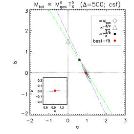
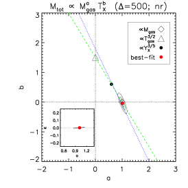
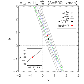
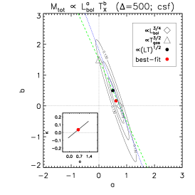
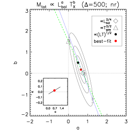
Figure 1: Contour plots that enclose 1.2, 1.5 and 2 times the minimum scatter, as function of the slopes $a$ and $b$ of the generalized scaling relations, as indicated in each panel. Also overplotted are the lines from eq. 2 (green dashed) and eq. 3 (blue dotted). (Top panels) The case of $\{A=M_{\rm gas},\;B=T\}$ using (from left to right) observational-like measurements of the xmas csf sample; direct measurements of the csf sample; direct measurements of the nr sample. (Bottom panels) The same as above, but for the case of $\{A=L,\;B=T\}$. The insets show the values of the normalization $K$ as a function of the slope $a$ in the region enclosed within 2 times the minimum scatter.

By combining these basic equations, we obtain that the scaling relations among the X-ray properties and the total mass are (see also Ettori et al. 2004):

• $E_{z}\;M_{\rm tot}\;\propto\;T^{3/2}$

• $M_{\rm tot}\;\propto\;M_{\rm gas}$

• $E_{z}\;M_{\rm tot}\;\propto\;(E_{z}^{-1}\;L)^{3/4}$.

Kravtsov et al. (2006) introduced the $Y_{X}$ mass proxy, which is given by the product of temperature and gas mass. Owing to its definition, it is related to the total thermal energy of the ICM. They demonstrated that, among the known mass indicators, $Y_{X}$ is a very robust mass proxy. Its scaling relation with $M_{500}$ being characterized by an intrinsic scatter of only 5–7 per cent at fixed $Y_{X}$, regardless of the dynamical state of the cluster and redshift, with a redshift evolution very close to the prediction of self-similar model. Arnaud et al. (2007) used XMM-Newton  data of a sample of 10 relaxed nearby clusters spanning a $Y_{X}$ range of $10^{13}-10^{15}M_{\odot}$ keV, and confirmed that the $M_{500}-Y_{X}$ relation has a slope close to the self-similar value of $3/5$, independent of the mass range considered. They showed that the normalisation of this relation is about 20 per cent below the prediction of numerical simulations which include cooling and supernova (SN) feedback, and explained this offset with two different effects: an underestimate of true mass due to a violation of the assumption of hydrostatic equilibrium, and an underestimate of hot gas mass fraction in the simulations (see also Zhang et al. 2008). They confirmed that $Y_{X}$ might indeed be a better mass proxy than $T$ and $M_{\rm gas}$ by comparing the functional form and scatter of the relations between different observables and mass. Extensive use of the $Y_{X}-M_{\rm tot}$ relation has been made in recent analyses aimed at constraining cosmological parameters through the evolution of the cluster mass function (e.g. Vikhlinin et al. 2009) and the properties of the scaling relations (Mantz et al. 2010). Pratt et al. (2009) presented the X-ray luminosity scaling relations of 31 nearby clusters from the Representative XMM-Newton  Cluster Structure Survey (REXCESS), all having temperature in the range 2–9 keV and selected in X-ray luminosity so as to properly sample the cluster luminosity function. Their analysis showed that scaling relations between bolometric X-ray luminosity and temperature, $Y_{X}$ and total mass, are all well represented by power–law shapes with slopes significantly steeper than self-similar predictions. They concluded that structural variations have little effect on the steepening, whereas it is largely affected by a systematic variation of the gas content with mass. Maughan (2007) analysed Chandra ACIS-I data for 115 galaxy clusters at $0.1<z<1.3$ observed to investigate the relation between luminosity and $Y_{X}$. They found that the scatter is dominated by cluster cores, and a tight $L_{X}-Y_{X}$ relation (11 per cent intrinsic scatter in $L_{X}$) is recovered if sufficiently large core regions ($0.15R_{500}$) are excluded. The tight correlation between $Y_{X}$ and mass and the self-similar evolution of that scaling relation out to $z=0.6$ is confirmed. Fabjan et al. (2011) analysed an extended set of cosmological simulations of galaxy clusters, and confirmed that the $M-Y_{X}$ scaling law is the least sensitive to variations of the physics in the ICM and very close, in terms of slope and evolution, to predictions of the self–similar model. They also pointed out that $M-M_{\rm gas}$ is the relation with the smallest scatter in mass, whereas $M-T$ is the one with the largest among the considered scaling relations.

In the present work, we generalise the definition of the $Y_{X}$ mass proxy, by considering the scaling relation between total mass, $M_{\rm tot}$, and a more general proxy defined in such a way that $M_{\rm tot}\propto A^{a}B^{b}$, where $A$ is either $M_{\rm gas}$ or $L$ and $B=T$. The use of this relation generalizes the relation $M_{\rm tot}-Y$, while maintaining the attitude to recover total mass by combining information on depth of the halo gravitational potential (through the gas temperature $T$) and distribution of gas density (traced by $M_{\rm gas}$ and X-ray luminosity), the latter being more affected by the physical processes determining the ICM properties. In doing that, we aim to minimize the scatter in the relations between total mass and observables by (i) relaxing the assumption of the self-similarity, (ii) adopting a general and flexible function with a minimal set of free parameters, (iii) offering a method that can be readjusted in dependence of the specific sample selection adopted.

In the recent past, similar work has been done by different authors with the aim of generalising the use of simple power-law scaling relations between cluster observables and total mass. Stanek et al. (2010) discussed the second moment of the halo scaling relations by investigating the signal covariance at fixed mass in numerical simulations. Okabe et al. (2010) used a small sample of 12 objects observed with Subaru and XMM-Newton  to study the covariance between the intrinsic scatter in $M_{\rm tot}–M_{\rm gas}$ and $M_{\rm tot}–T$ relations and to propose a method to identify a robust mass proxy based on principal component analysis. Rozo et al. (2010) presented an extensive discussion on the relaxation of some assumptions on the parametrization of the relation between optical richness and total mass, by introducing the possibility of deviation from a power–law shape, as well as richness– and mass–dependence of intrinsic scatter.

To study the behaviour of the $M_{\rm tot}\;\propto\;A^{a}B^{b}$ relation in minimizing the scatter, we used a sample of 24 Lagrangian regions, selected around the most massive clusters with a radius equal to five times the virial radius, and extracted from a parent low-resolution N-body cosmological simulation with a box of size 1$\,h^{-1}$Gpc comoving, as described in Bonafede et al. (2011). A flat $\Lambda$CDM cosmological model with $\Omega_{m}=0.24$, $\Omega_{bar}=0.04$, $n_{s}=0.96$, $\sigma_{8}=0.8$ and present day Hubble constant of 72 km s^-1 Mpc^-1, consistent with WMAP-7 cosmological parameters (Komatsu et al. 2011), was assumed. A set of 24 Lagrangian regions, centred around as many massive clusters, were re-simulated by increasing mass resolution and adding high-frequency modes to the power spectrum (Tormen et al. 1997). Within the high resolution region, dark matter particles have a mass $m_{DM}=8.47\times 10^{8}$ $h^{-1}$ $M_{\odot}$. The size of each Lagrangian region was chosen in such a way that by $z=0$ there are no low–resolution particles within at least 5 virial radii from the central cluster. As a result, the large extent of each of these high–resolution regions allows one to identify more than one single cluster–sized halo within it, which is not contaminated by low–resolution particles within its virial region (Bonafede et al. 2011; Fabjan et al. 2011).

Clusters identified from this set of initial conditions were simulated with the TreePM-SPH GADGET-3 code, an improved version of the original GADGET-2 code (Springel 2005). As described by Fabjan et al. (2011), simulations have been carried out for two different prescriptions for the physics determining the evolution of cosmic baryons: (i–sample nr) non–radiative physics and (ii–sample csf) including metallicity–dependent radiative cooling, a model for star formation and galactic winds triggered by SN explosions (as described by Springel & Hernquist 2003) with velocity $v_{w}=500$ km s^-1, and a detailed model of chemical evolution as described by Tornatore et al. (2007). By selecting only objects with mass weighted temperature $T>2$ keV, we end up with 41 objects in each sample. A subset of the csf sample has been processed through the X-MAS tool (e.g. Rasia et al. 2008) to generate Chandra mock observations, and then analyzed with an observational-like approach to measure temperatures and gas masses (xmas sample; Rasia et al. 2011). The latter sample includes all the clusters with spectroscopic-like temperature larger than 2 keV, and observed along 3 orthogonal projection directions, so that we end up with 159 mock observations of simulated clusters. Total and gas masses within $R_{500}$ are computed as as described in Fabjan et al. (2011) and Rasia et al. (2011). Gas temperatures and luminosities, both bolometric and in the 0.1-2.4 keV band, are computed after excising cluster core regions, which are defined as the regions enclosed within $0.15R_{500}$. The effect of core excision is also considered in the discussion of the results and is shown not to affect the conclusions of our analysis.

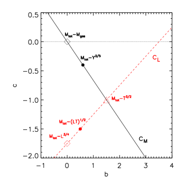
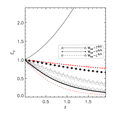
Figure 2: Evolution of the scaling relation parametrized through the quantity $E_{z}$ in the SS scenario and including the relations in equation 2. Solid (dashed) lines show the behaviour for the relations with $A=M_{\rm gas}$ ($A=L$). (Left) Values of $c$, exponent of $E_{z}$, from equation 4 as function of the logarithmic slope $b$ ($c=0$ in the case of no-evolution). (Right) Values of $E_{z}^{c}$ as function of the redshift for different scaling relations. As representative cases, two sets of lines are plotted: thin lines assume $b=-1$, thick lines adopt $b=3$.

We fit a linear relation to the log-log scaling between total mass and proxies, normalized to the average values computed within each sample of simulated clusters:

$$\log_{10}\hat{M}_{\rm tot}=K+a\log_{10}\hat{A}+b\log_{10}\hat{B},.$$ (1)

Here we defined $\{\hat{M}_{\rm tot}=M_{\rm tot}/\bar{M}_{\rm tot},\hat{A}=A/\bar{A},\hat{B}=B/\bar{B}\}$, with barred quantities indicating the average values of the corresponding quantities.

Within each set of simulated clusters, containing N objects, we compute for each pair of values of the slopes $\{a_{i},b_{j}\}$ the corresponding scatter, which is defined as $\sigma^{2}(a_{i},b_{j})=\sum_{k=1,N}(\log_{10}\hat{M}_{\rm tot,k}-\hat{K}-a_{i}\log_{10}\hat{A}_{k}-b_{j}\log_{10}\hat{B}_{k})^{2}/N$, where $\hat{K}=\sum_{k=1,N}(\log_{10}\hat{M}_{\rm tot,k}-a_{i}\log_{10}\hat{A}_{k}-b_{j}\log_{10}\hat{B}_{k})/N$. We then search find the locus in the $\{a,b\}$ plane where scatter is minimized in a similar. In all cases, this locus is well represented by the lines

$$\{A=M_{\rm gas},\;B=T\}\Rightarrow \;b_{M}=-3/2a_{M}+3/2$$

$$\{A=L,\;B=T\}\Rightarrow \;b_{L}=-2a_{L}+3/2,$$ (2)

(see Fig. 1) or, in a more concise form, $b=-(1+1/2d)\,a+3/2$, where $d$ corresponds to the power to which the gas density appears in the formula of the gas mass ($d=1$) and luminosity ($d=2$). This correlation between logarithmic slopes allows us to reduce by one the number of free parameter in the linear fit of the generalized scaling law between observables and total mass.

It is worth noticing that these relations reduce to the standard self-similar predictions in the appropriate cases: $M_{\rm tot}\propto T^{3/2}$, $M_{\rm tot}\propto M_{\rm gas}$, $M_{\rm tot}\propto Y^{3/5}$ are recovered for $a_{M}=0,1$ and $3/5$, respectively; $M_{\rm tot}\propto L^{3/4}$ and $M_{\rm tot}\propto\left(LT\right)^{1/2}$, which is the corresponding relation of $M_{\rm tot}\propto Y^{3/5}$ once gas mass is replaced by luminosity, are recovered for $a_{L}=3/4$ and $1/2$, respectively.

However, to represent the tilted shape of the contours encircling the region with the minimum scatter in the simulated dataset here investigated, we should prefer the following relations among the logarithmic slopes,

$$b_{M}\approx-1.9a_{M}+1.8,\;b_{L}\approx-2.4a_{L}+1.8,$$

$$b\approx-(1.4+0.5\,d)\,a+1.8$$ (3)

that are shown as dotted lines in Fig. 1.

In the following discussion, we refer to the SS case described from the equations 2 as the reference one.

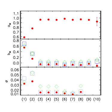
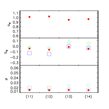
Figure 3: Best-fit values of the slopes $a_{M}$ and $b_{M}$ as a function of the sample examined, (1)-(10) from xmas (Rasia et al. 2011), (11)-(14) from direct measurements in the hydrodynamical simulations (Fabjan et al. 2011): (1) at $\Delta=2500$, with the spectroscopic-like estimate $T=T_{\rm sl}>2$ keV; (2) at $\Delta=2500$, with the X-ray spectroscopically determined $T=T_{\rm X}>2$ keV; (3) with $T=T_{\rm X}>2$ keV and the core included; (4) with $T=T_{\rm sl}>2$ keV; (5) with $T=T_{\rm X}>2$ keV; (6) with $T=T_{\rm sl}>4$ keV; (7) with $T=T_{\rm X}>4$ keV; (8) with $M_{\rm tot}>10^{14}M_{\odot}$; (9) with $T=T_{\rm X}$ and 1,000 realizations of randomly selected objects with 30 clusters with $2<T<4$ keV and 40 clusters with $4<T<10$ keV; (10) the same as in (9) but including a relative statistical error of 20 per cent on the total mass; (11) for the sample nr and excluding the core ($0-0.15R_{500}$), (12) including the core, (13) for the sample csf and excluding the core, (14) including the core. For the cases (3)-(14), all quantities are estimated at $\Delta=500$. The bottom panels show the corresponding scatter $\sigma$. Green diamonds and blue squares in the central (lower) panels are the predicted slope $b_{M}$ (scatter) from the SS relations in equation 2 and the corrected relations in eq. 3, respectively.

3 Evolution, normalization and robustness of the generalized scaling laws

In this section, we discuss some properties on the redshift evolution and normalization of the generalized scaling laws, and present the results of the tests by which we have verified the robustness of our predictions.

3.1 Evolution of the generalized scaling laws

With simple mathematical substitutions, we can predict the redshift evolution expected for the SS case, $M_{\rm tot}\;\propto\;E_{z}^{c}$:

$$\{A=M_{\rm gas},\;B=T\}\Rightarrow \;c_{M}=-2/3b_{M}=a_{M}-1$$

$$\{A=L,\;B=T\}\Rightarrow \;c_{L}=b_{L}/2-7/4=-a_{L}-1.$$ (4)

We are now in the position to look for the scaling relation which has the weakest redshift dependence or, on the contrary, the relation which makes this dependence stronger. We note that there is no dependence on redshift only in two cases among the scaling relations here investigated (see Fig. 2): (i) $a_{M}=1$ (and $b_{M}=0$), i.e. for the scaling law $M_{\rm tot}\propto M_{\rm gas}$; (ii) $a_{L}=-1$ (and $b_{L}=7/2$), i.e. for the relation $M_{\rm tot}\propto L^{-1}T^{7/2}$. The prediction for the lack of evolution of these scaling relations can be tested against observational data.

3.2 Normalization of the generalized scaling laws

As shown in Fig. 1, the normalization $K$ corresponding to the value of minimum scatter is close to zero. This is expected once the quantities are normalized to the averaged values $\bar{M}_{\rm tot},\bar{A},\bar{B}$. However, only $\bar{A}$ and $\bar{B}$ are known for an observed sample. Thus, by adopting one of the relations in equation 2, one can directly measure $\hat{M}_{\rm tot}=M_{\rm tot}/\bar{M}_{\rm tot}$ and recover the total mass $M_{\rm tot}$ only once $\bar{M}_{\rm tot}$ is independently evaluated either through mock samples selected from catalogs of hydrodynamically simulated objects to contain the same number of objects, and with similar properties, of the observed ones, or through a self–calibration tuned by a sub-sample of clusters for which robust mass estimates are available. Under this respect, the suggested approach is the standard one, with the same limitations affecting any other application of the scaling laws: mass calibration and selection effects. The innovation, we are proposing, is to add an extra parameter, imposing a new constraint on the slopes of the scaling laws, to allow a further minimization of the scatter.

3.3 Robustness of the generalized scaling laws

To assess the robustness of the analysis of the simulated dataset, we have repeated our calculations by extracting the simulated objects according to different criteria, e.g., including or excluding the cluster core emission, adopting different overdensity, using different definition for the gas temperature, selecting only very hot or massive systems. All these samples reproduce consistently the plots shown in Fig. 1, by varying only the location of the best-fit values, but confirming the dependence among the logarithmic slopes over the region of the parameter space that minimize the measured scatter (see Fig. 3).

When observational data are considered, several other selection effects can still affect both the definition of a sample and the measurements of the normalization and slope of the adopted scaling law. A proper treatment of the second–order moments and of the covariance related to the scaling relation has then to be addressed (see, e.g., Stanek et al. 2010, Rozo et al. 2009 and 2010, Mantz et al. 2010).

4 Summary and discussion

We have presented new generalized scaling relations with the prospective to reduce further the scatter between mass proxies and total cluster mass. We find a locus of minimum scatter that relates the logarithmic slopes of the two independent variables considered in the present work, namely temperature $T$, which traces the depth of the cluster potential, and another one accounting for the gas density distribution, such as gas mass $M_{\rm gas}$ or X-ray luminosity $L$. Within this approach, all the known scaling relations appear as particular realizations of generalized scaling relations. For instance, we introduced the scaling relation $M_{\rm tot}\propto(LT)^{1/2}$, which is analogous to the $M_{\rm tot}-Y$ relation, once luminosity is used instead of gas mass.

Also the evolution expected in the framework of the self-similar model are predicted for the generalized scaling relations. They can be used either to maximize the evolutionary effect to test predictions of the self-similar models itself or, on the contrary, to minimize them in case of cosmological applications.

A linear function in the logarithmic space can be then fitted to the data normalized to the average values measured in the sample:

$$\log_{10}\hat{M}_{\rm tot}=K+a\log_{10}\hat{A}+b\log_{10}\hat{B}+c\log_{10}E_{z},$$ (5)

with $K=0$, $b_{M}=-3/2a_{M}+3/2$, $c_{M}=-2/3b_{M}=a_{M}-1$ for $\{A=M_{\rm gas},B=T\}$ and $K=0$, $b_{L}=-2a_{L}+3/2$, $c_{L}=b_{L}/2-7/4=-a_{L}-1$ for $\{A=L,B=T\}$. In a more concise form, the above relation can be recast as $b=-(1+1/2\,d)\,a+3/2$, where $d$ corresponds to the power with which gas density appears to define either gas mass ($d=1$) or luminosity ($d=2$). This fitting function has 4 free parameters that are reduced to one (plus the average value of the total mass of the objects in the sample) thanks to the existing tight correlation found between $a$ and $b$, at least within the region of the $\{a,b\}$ parameter space where intrinsic scatter is minimised.

The method and the results presented in this work offer a robust framework to relate, with the request of a minimum scatter, the X-ray observables to the total gravitational mass of galaxy clusters for studies of their thermodynmical properties and for cosmological application.

References

- [] Allen, S. W., Evrard, A. E., & Mantz, A. B. 2011, ARAA, 49, 409
- [1] Arnaud M., Pointecouteau E., Pratt G.W., 2007, A&A, 474, L37
- [] Bonafede A. et al, 2011, MNRAS, in press (arXiv:1107.0968)
- [] Borgani, S., & Kravtsov, A. 2009, arXiv:0906.4370
- [] Ettori S. et al., 2004, MNRAS, 354, 111
- [] Evrard A.E., Henry J.P., 1991, ApJ, 383, 95
- [] Fabjan D., Borgani S., Rasia E., Bonafede A., Dolag K., Murante G., Tornatore L., 2011, MNRAS (in press, arXiv:1102.2903)
- [] Kaiser N., 1986, MNRAS, 222, 323
- [] Kaiser N., 1991, ApJ, 383, 104
- [] Komatsu E. et al., 2011, ApJS, 192, 18
- [] Kravtsov A.V., Vikhlinin A., Nagai D., 2006, ApJ, 650, 128
- [] Mantz A. et al., 2010, MNRAS, 406, 1773
- [] Mathiesen B.F., Evrard A.E., 2001, ApJ, 546, 100
- [] Maughan B.J., 2007, ApJ, 668, 772
- [] Okabe N. et al., 2010, ApJ, 721, 875
- [] Pratt G.W., Croston J.H., Arnaud M., Böhringer H., 2009, A&A, 498, 361
- [] Short C.J., Thomas P.A., Young O.E., Pearce F.R., Jenkins A., Muanwong O., 2010, MNRAS, 408, 2213
- [] Rasia E. et al., 2008, ApJ, 674, 728
- [] Rasia E., Meneghetti M., Martino R., Borgani S., Bonafede A. et al. 2011, preprint
- [] Rozo E. et al., 2009, ApJ, 699, 768
- [] Rozo E. et al., 2010, ApJ, 708, 645
- [] Springel V., Hernquist L., 2003, MNRAS, 339, 289
- [] Springel, V. 2005, MNRAS, 364, 1105
- [] Stanek R., Rasia E., Evrard A.E., Pearce F., Gazzola L., 2010, ApJ, 715, 1508
- [] Tormen G., Bouchet F. R., White S. D. M., 1997, MNRAS, 286, 865
- [] Tornatore L. et al., 2007, MNRAS, 382, 1050
- [] Vikhlinin A. et al., 2009, ApJ, 692, 1033
- [] Voit, G. M. 2005, Rev. Mod. Phys., 77, 207
- [] Zhang Y.-Y. et al., 2008, A&A, 482, 451