Dynamo models of grand minima

Abstract

Since a universally accepted dynamo model of grand minima does not exist at the present time, we concentrate on the physical processes which may be behind the grand minima. After summarizing the relevant observational data, we make the point that, while the usual sources of irregularities of solar cycles may be sufficient to cause a grand minimum, the solar dynamo has to operate somewhat differently from the normal to bring the Sun out of the grand minimum. We then consider three possible sources of irregularities in the solar dynamo: (i) nonlinear effects; (ii) fluctuations in the poloidal field generation process; (iii) fluctuations in the meridional circulation. We conclude that (i) is unlikely to be the cause behind grand minima, but a combination of (ii) and (iii) may cause them. If fluctuations make the poloidal field fall much below the average or make the meridional circulation significantly weaker, then the Sun may be pushed into a grand minimum.

1 Introduction

At the very outset, I would like to mention that the subject of this invited talk was not chosen by me. The organizers felt that this symposium should have an invited talk on dynamo models of grand minima and requested me to give it. Only after considerable initial hesitation, I finally agreed. The reason behind my initial hesitation is that at present we have no dynamo model of grand minima which is completely satisfactory or which is generally accepted in the community. No two self-respecting dynamo theorists seem to agree how grand minima are produced! To the best of my knowledge, this is the first time an invited talk on this subject is being given in a major international conference.

Given this situation, I have decided to adopt the following strategy. I shall mainly focus on the various bits of physics which go into making models of grand minima rather than discussing specific models of grand minima in detail. While many of the present-day models of grand minima may eventually fall by the wayside, I believe that the bits of physics that we consider relevant today will still remain relevant after 20 or 30 years when there may be a better understanding of what occasionally pushes the Sun into the grand minima.

2 Observational characteristics of grand minima

Before getting into the theoretical discussion, let us see what we can learn about the characteristics of grand minima from the very limited observational data available to us.

Several authors have studied the archival records of sunspots during the Maunder minimum (Sokoloff & Nesme-Ribes 1994; Hoyt & Schatten 1996). The few sunspots seen during the Maunder minimum mostly appeared in the southern hemisphere. Sokoloff & Nesme-Ribes (1994) have used the archival data to construct a butterfly diagram for a part of the Maunder minimum from 1670, showing a clear trend of hemispheric asymmetry. It is an open question whether hemispheric asymmetry played any crucial role in creating the Maunder minimum (Charbonneau 2005). Usoskin, Mursula & Kovaltsov (2000) argued that the Maunder minimum started abruptly but ended in a gradual manner, indicating that the strength of the dynamo must be building up as the Sun came out of the Maunder minimum. However, some recent evidence suggests that the onset of the Maunder minimum may not be as abrupt as believed earlier (Vaquero et al. 2011).

When solar activity is stronger, magnetic fields in the solar wind suppress the cosmic ray flux, reducing the production of ¹⁰Be and ¹⁴C which can be used as proxies for solar activity. From the analysis of ¹⁰Be abundance in a polar ice core, Beer, Tobias & Weiss (1998) concluded that the solar activity cycle continued during the Maunder minimum, although the overall level of the activity was lower than usual. Miyahara et al. (2004) drew the same conclusion from their analysis of ¹⁴C abundance in tree rings.

This method of using various proxies (like the abundances of ¹⁰Be and ¹⁴C) for sunspot activity can be extended to study even the earlier grand minima before the Maunder minimum. Usoskin, Solanki & Kovaltsov (2007) estimated that there have been about 27 grand minima in the last 11,000 years. They also identified about 19 grand maxima, i.e. periods during which sunspot activity was unusually high, like what was seen during much of the twentieth century.

3 Are grand minima merely extremes of cycle irregularities?

We know that the solar cycle is only approximately periodic. Both the strength and the period vary from one cycle to another. We begin our theoretical discussion by raising the question whether the grand minima are merely extreme examples of cycle irregularities. Are the theoretical ideas used to model irregularities of solar cycles adequate to explain the occurrences of grand minima, or do we need to invoke some qualitatively different ideas? We do not yet have a definitive answer to this question. Any dynamo theorist is entitled to have his or her own personal opinion. Let me put forth my personal opinion.

Our simulations (to be discussed later) seem to suggest that nothing very extraordinary may be needed to push the Sun into a grand minimum. If the fluctuations which cause the usual cycle irregularities are sufficiently large, they may sometimes cause grand minima. However, even after the Sun is pushed into the grand minimum, a subdued cycle has to continue (as discussed in § 2) and eventually the Sun has to come out of the grand minimum. These are more problematic to explain. There are certain mechanisms of magnetic field generation which crucially depend on the existence of sunspots. Certainly those mechanisms cannot be operative during a grand minimum. So we need to invoke alternative mechanisms.

Let us look at the question how magnetic fields are generated in the dynamo process. The basic idea of solar dynamo is that the toroidal and poloidal components of the solar magnetic field sustain each other through a feedback loop. It is fairly easy to generate the toroidal field by the stretching of the poloidal field due to differential rotation. Since helioseismology has shown that the differential rotation is concentrated in the tachocline, the generation of toroidal field mainly takes place there. To complete the loop, we need to generate the poloidal field from the toroidal field. The historically important idea of Parker (1955) — which was further elaborated by Steenbeck, Krause & Rädler (1966) — is that the cyclonic turbulence in the convection zone twists the toroidal field to produce the poloidal field. This mechanism is often called the $\alpha$-effect because the crucial parameter describing this process is usually denoted by the symbol $\alpha$. Within certain approximation schemes, this parameter can be shown to be given by

$$\alpha=-\,\frac{1}{3}\,\overline{\bf v.(\nabla\times\bf v)}\;\tau,$$

where $\bf v$ is the fluctuating part of the velocity field and $\tau$ is the correlation time (see, for example, Choudhuri 1998, § 16.5). This $\alpha$-effect mechanism can be operative only if the toroidal field is not too strong such that the helical turbulence is able to twist it. However, the flux tube rise simulations by several authors (Choudhuri & Gilman 1987; Choudhuri 1989; D’Silva & Choudhuri 1993; Fan, Fisher & DeLuca 1993; Caligari et al. 1995) indicated that the toroidal field at the base of the solar convection zone has to be as strong as $10^{5}$ G. Such a strong field cannot be twisted by helical turbulence and we cannot invoke $\alpha$-effect to generate the poloidal field from such a strong toroidal field. An alternative mechanism which has been widely used in many recent dynamo simulations is due to Babcock (1961) and Leighton (1969). Bipolar sunspots on the solar surface have a tilt with respect to the solar equator and this tilt increases with latitude. This was discovered by Joy in 1919 and is known as Joy’s law. D’Silva & Choudhuri (1993) provided the first theoretical explanation of Joy’s law by showing that the tilt is produced by the Coriolis force acting on the flux tubes rising through the convection zone due to magnetic buoyancy. When a tilted bipolar sunspot decays, fluxes of opposite polarities diffuse at slightly different latitudes, contributing to the poloidal field. According to this Babcock–Leighton mechanism, a tilted bipolar sunspot pair is a conduit for converting the toroidal field to the poloidal field. The sunspot pair forms due to the buoyant rise of the toroidal field and we get the poloidal field after its decay.

Since we see the Babcock–Leighton mechanism clearly operational at the solar surface, most of the recent flux transport dynamo models take this as the primary generation mechanism of the poloidal field. The $\alpha$-effect cannot operate on the strong toroidal field at the base of the convection zone. But this strong toroidal field is expected to be highly intermittent (Choudhuri 2003) and the $\alpha$-effect is likely to be operative in those regions of the convection zone where the toroidal field is weak, although the nature, the spatial distribution and even the algebraic sign of the $\alpha$ parameter remain unclear at the present time. The Babcock–Leighton mechanism presumably cannot work during the grand minimum when there are no sunspots. So we have to fall back upon the $\alpha$-effect to continue the cycles during the grand minimum and eventually to pull the Sun out of it. Our lack of knowledge about the $\alpha$-process limits our understanding of these phenomena. In the mean field dynamo equations, the term capturing the Babcock–Leighton process is formally very similar to the term capturing the $\alpha$-effect — often even using the symbol $\alpha$. Hence many dynamo models of the grand minima are worked out at the present time by solving the same equations during and outside the grand minima. But it should be kept in mind that the physics behind the symbol $\alpha$ must be very different during and outside the grand minima.

In summary, our view is that the usual sources of irregularities in solar cycles are sufficient for the onset of a grand minimum, but to pull the Sun out of a grand minimum we need some physics different from the physics behind the usual solar cycles. Presumably the situation is somewhat different for grand maxima. Not only are the usual irregularities expected to cause a grand maximum, we also do not require anything unusual to take the Sun out of the grand maximum. The usual poloidal field generation by the Babcock–Leighton mechanism continues during the grand maximum. It is intriguing that Usoskin, Solanki & Kovaltsov (2007) concluded that the lengths of grand maxima correspond to an exponential distribution, but the lengths of grand minima have a more complicated bimodal distribution. Is this connected with the fact that grand maxima do not involve any physical processes different from the normal, but grand minima require the generation process of the poloidal field to be different from the normal situation?

4 The origin of irregularities in the flux transport dynamo

We now discuss the possible sources of irregularities in the flux transport dynamo — the most widely studied model of the solar cycle in recent years. Let us begin by recapitulating some basic facts about the flux transport dynamo. The toroidal field is generated in the tachocline by the strong differential rotation and then rises to the surface due to magnetic buoyancy to form tilted bipolar sunspots. When these sunspots decay, we get the poloidal field by the Babcock–Leighton mechanism. The meridional circulation of the Sun, which is found to be poleward in the upper layers of the convection zone and must have a hitherto unobserved equatorward branch at the bottom of the convection zone in order to conserve mass, plays a very crucial role in the flux transport dynamo. The meridional circulation causes the observed poleward transport of the poloidal field. At the base of the convection zone, it is responsible for making the dynamo wave propagate equatorward, such that sunspots are produced at lower and lower latitudes with the progress of a cycle. In the absence of the meridional circulation, the dynamo wave at the bottom of the convection zone would propagate poleward in accordance with the Parker–Yoshimura sign rule (Parker 1955; Yoshimura 1975) contradicting observations. The flux transport dynamo could become a serious model of the solar cycle only after Choudhuri, Schüssler & Dikpati (1995) demonstrated that a sufficiently strong meridional circulation could overrule the Parker–Yoshimura sign rule and make the dynamo wave propagate in the correct direction.

The original flux transport dynamo model of Choudhuri, Schüssler & Dikpati (1995) led to two offsprings: a high diffusivity model and a low diffusivity model. The diffusion times in these two models are of the order of 5 years and 200 years respectively. The high diffusivity model has been developed by a group working in IISc Bangalore (Choudhuri, Nandy, Chatterjee, Jiang, Karak), whereas the low diffusivity model has been developed by a group working in HAO Boulder (Dikpati, Charbonneau, Gilman, de Toma). The differences between these models have been systematically studied by Jiang, Chatterjee & Choudhuri (2007) and Yeates, Nandy & Mckay (2008). Both these models are capable of giving rise to oscillatory solutions resembling solar cycles. However, when we try to study the irregularities of the cycles, the two models give completely different results. We need to introduce fluctuations to cause irregularities in the cycles. In the high diffusivity model, fluctuations spread all over the convection zone in about 5 years. On the other hand, in the low diffusivity model, fluctuations essentially remain frozen during the cycle period. Thus the behaviours of the two models are totally different on introducing fluctuations. Over the last few years, several independent arguments have been advanced in support of the high diffusivity model (Chatterjee, Nandy & Choudhuri 2004; Chatterjee & Choudhuri 2006; Jiang, Chatterjee & Choudhuri 2007; Goel & Choudhuri 2009; Hotta & Yokoyama 2010). We adopt the point of view here the solar dynamo is most likely a high diffusivity flux transport dynamo.

Three main sources of irregularities in dynamo models have been studied by different authors over the years: (i) chaotic behaviours introduced by nonlinearities of the dynamo process; (ii) fluctuations in the generation of the poloidal field; (iii) fluctuations in the meridional circulations. The three following sections will focus on these three sources of irregularities and discuss the question whether they can cause grand minima. Some of these sources of irregularities have been investigated even before the flux transport dynamo model became popular, by applying them to the earlier solar dynamo models.

5 Effects of nonlinearities

It is well known that nonlinear dynamical systems can show complicated chaotic behaviours. Some of the earliest efforts of modelling solar cycle irregularities invoked the idea of nonlinear chaos. The full dynamo problem is certainly a nonlinear problem in which the magnetic fields produced by the fluid motions react back on the fluid motions. The simplest way of capturing the effect of this in a kinematic dynamo model (in which the fluid equations are not solved) is to consider a quenching of the $\alpha$ parameter as follows:

$$\alpha=\frac{\alpha_{0}}{1+|\overline{B}/B_{0}|^{2}},$$

where $\overline{B}$ is the average of the magnetic field produced by the dynamo and $B_{0}$ is the value of magnetic field beyond which nonlinear effects become important. There is a long history of dynamo models studied with such quenching (Stix 1972; Ivanova & Ruzmaikin 1977; Yoshimura 1978; Brandenburg et al. 1989; Schmitt & Schüssler 1989). In most of the nonlinear calculations, however, the dynamo eventually settles to a periodic mode with a given amplitude rather than showing sustained irregular behaviour. The reason for this is intuitively obvious. Since a sudden increase in the amplitude of the magnetic field would diminish the dynamo activity by reducing $\alpha$ given by (2) and thereby pull down the amplitude again (a decrease in the amplitude would do the opposite), the $\alpha$-quenching mechanism tends to lock the system to a stable mode once the system relaxes to it. In fact, Krause & Meinel (1988) and Brandenburg et al. (1989) argued that the nonlinear stability may determine the mode in which the dynamo is found. Yoshimura (1978) was able to reproduce some irregular features of the solar cycle by introducing an unrealistic delay time of 29 years between the magnetic field and its effect on the $\alpha$-coefficient. In some highly truncated models with the suppression of differential rotation, one could find the evidence of chaos in limited parts of the parameter space (Weiss, Cattaneo & Jones 1984). Küker, Arlt & Rüdiger (1999) suggested that the quenching of differential rotation might have caused the Maunder minimum. This seems unlikely now on the ground that torsional oscillations — periodic modulations of differential rotation caused by the dynamo-generated magnetic field — appear like small perturbations.

It does not seem that the irregularities of solar cycles are primarily caused by nonlinearities. But that does not mean that nonlinearities have no important consequences in the currently favoured flux transport dynamo models. In order to explain the even-odd or the Gnevyshev–Ohl effect of solar cycles, Charbonneau, St-Jean & Zacharias (2005) and Charbonneau, Beaubien & St-Jean (2007) made the highly provocative suggestion that the solar dynamo may be sitting in a region of period doubling just beyond the point of nonlinear bifurcation. Recently the effects of nonlinearities introduced by the quenching of turbulent diffusion (Guerrero, Dikpati & de Gouveia Dal Pino 2009) and meridional circulation (Karak & Choudhuri 2012) are being investigated.

6 Fluctuations in poloidal field generation

Since the mean field dynamo equations are derived by averaging over turbulence, we expect fluctuations to be present around the mean. Choudhuri (1992) was the first to suggest that these fluctuations will be particularly important in the poloidal field generation. It is now difficult to believe that this was an unorthodox and radical idea in 1992 when it was proposed, though this idea was explored further by Moss et al. (1992), Hoyng (1993) and Ossendrijver, Hoyng & Schmitt (1996). This idea was applied to the flux transport dynamo by Charbonneau & Dikpati (2000).

Let us consider the question how fluctuations in poloidal field generation arise in the flux transport dynamo. The Babcock–Leighton mechanism of poloidal field generation depends the tilts of bipolar sunspot pairs. While the average tilts are given by Joy’s law, one finds a large scatter around this average. Longcope & Choudhuri (2002) provided a theoretical model of this scatter on the basis of the idea that the rising flux tubes are buffeted by turbulence in the convection zone. This scatter around Joy’s law produces fluctuations in the poloidal field generation process and we identify this as a primary source of irregularities in the solar cycle. It may be noted that Choudhuri, Chatterjee & Jiang (2007) and Jiang, Chatterjee & Choudhuri (2007) modelled the last few cycles by assuming the fluctuations in poloidal field generation to be the main source of irregularities in solar cycles and predicted that the forthcoming cycle 24 will be weak. This prediction was based on the high diffusivity model. There are enough indications by now that the upcoming cycle is going to be a weak one, providing further support to the high diffusivity model.

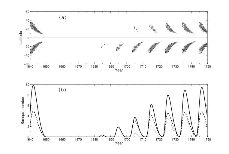
Figure 1: The theoretical model of the Maunder minimum from Choudhuri & Karak (2009). This is based on a simulation in which the poloidal field was reduced to 0.0 and 0.4 of its average value in the two hemispheres. The upper panel shows the butterfly diagram. The dotted and dashed lines in the lower panel are sunspot numbers in the northern and southern hemispheres, whereas the solid line is their sum.

We now come to question whether fluctuations in the poloidal field generation can produce grand minima. Several authors found that intermittencies resembling grand minima can be obtained in simple dynamo models by introducing fluctuations (Schmitt, Schüssler & Ferriz-Mas 1996; Mininni, Gomez & Mindlin 2001; Brandenburg & Spiegel 2008). The effect of such fluctuations on flux transport dynamo models has been investigated only recently. Charbonneau, Blais-Laurier & St-Jean (2004) carried out a simulation by introducing 100% fluctuations in $\alpha$ (the poloidal field generation parameter) in a flux transport dynamo with low diffusivity. They found intermittencies in their simulations resembling grand minima. The low diffusivity of their model ensured that the diffusive decay time or the ‘memory’ of the dynamo was rather long (of the order of a century) and most probably this long memory played a role in producing intermittencies of similar duration. The important question is whether the high diffusivity dynamo model, which we consider to be the appropriate model for explaining solar cycles and which has a much smaller diffusive decay time, can also produce similar intermittencies on introducing fluctuations in poloidal field generation. This question has been studied by Choudhuri & Karak (2009).

Choudhuri, Chatterjee & Jiang (2007) proposed a simplified procedure for incorporating the cumulative effect of fluctuations in poloidal field generation. Since these fluctuations in poloidal field generation would make the poloidal field at the end of a cycle different from the average poloidal field one would get from the mean field equations without including fluctuations, they suggested that the poloidal field at the end of the cycle may be modified suitably to account for the cumulative effect of the fluctuations. Choudhuri & Karak (2009) found that the dynamo is pushed into a grand minimum if the poloidal field at the end of a cycle falls to 0.2 of its average value. At the time of this work during the depth of a long sunspot minimum, there was considerable speculation whether the Sun was entering another grand minimum. Choudhuri & Karak (2009) concluded that the poloidal field had fallen to only about 0.6 of its average value and hence the Sun should not be entering another grand minimum. On making the poloidal field in the northern and southern hemispheres fall to respectively 0.0 and 0.4 of its average value, Choudhuri & Karak (2009) found that many characteristics of the Maunder minimum were reproduced. Fig. 1 shows the theoretical plots of butterfly diagram and sunspot number, which compare favourably with the corresponding observational plots given in Fig. 1(a) of Sokoloff & Nesme-Ribes (1994) and Fig. 1 of Usoskin, Mursula & Kovaltsov (2000). We find that the theoretical model reproduced the fact that the Maunder minimum started abruptly, but ended gradually. It is basically the growth time of the dynamo which determines the duration of the grand minimum during which the magnetic field has to grow up again to return to normalcy. As pointed out in § 3, the operation of the dynamo during the grand minimum presumably depends on the $\alpha$-effect and the theoretical model shows an ongoing but subdued cycle of magnetic field in the solar wind. We sum up the theoretical results in the following words. If the poloidal field at the end of a cycle turns out to be very weak due to fluctuations in its generation process, then that can push the dynamo into a grand minimum, from which it recovers gradually in the dynamo growth time.

7 Fluctuations in meridional circulation

It is well known that the period of the flux transport dynamo varies roughly as the inverse of the meridional circulation speed. The period of the dynamo is approximately given by the time taken by meridional circulation at the bottom of the convection zone to move from higher latitudes to lower latitudes. In other words, the period of a flux transport dynamo does not depend too much on the details of poloidal field generation mechanism. Probably this is the reason why the period of the dynamo during a grand minimum like the Maunder minimum does not change drastically, even though the poloidal field generation mechanism may be different from normal times as explained § 3.

Since the meridional circulation determines the period of the flux transport dynamo, it is obvious that any fluctuations in meridional circulation would have an effect on the flux transport dynamo. It has been found recently that the meridional circulation has a periodic variation with the solar cycle, becoming weaker at the time of sunspot maximum (Hathaway & Rightmire 2010; Basu & Antia 2010). Presumably the Lorentz force of the dynamo-generated magnetic field slows down the meridional circulation at the time of the sunspot maximum. Karak & Choudhuri (2012) found that this quenching of meridional circulation by the Lorentz force does not produce irregularities in the cycle, provided the diffusivity is high as we believe. We disagree with the model of Nandy, Muñoz-Jaramillo & Martens (2011) which assumes that the meridional circulation changes abruptly at each sunspot maximum. Our point of view is that the periodic variation of meridional circulation due to the Lorentz force cannot be responsible for solar cycle irregularities and we need to consider other kinds of fluctuations in meridional circulation.

We have reliable observational data on the variation of meridional circulation only for a little more than a decade. To draw any conclusions about the variation of meridional circulation at earlier times, we have to rely on indirect arguments. If we assume the cycle period to go inversely as meridional circulation, then we can use periods of different past solar cycles to infer how meridional circulation has varied with time in the last few centuries. On the basis of such considerations, it appears that the meridional circulation had random fluctuations in the last few centuries with correlation time of the order of 30–40 years (Karak & Choudhuri 2011). We now come to question what effect these random fluctuations of meridional circulation may have on the dynamo. Based on the analysis of Yeates, Nandy & Mckay (2008), we can easily see that dynamos with high and low diffusivity will be affected very differently. Suppose the meridional circulation has suddenly fallen to a low value. This will increase the period of the dynamo and lead to two opposing effects. On the one hand, the differential rotation will have more time to generate the toroidal field and will try to make the cycles stronger. On the other hand, diffusion will also have more time to act on the magnetic fields and will try to make the cycles weaker. Which of these two competing effects wins over will depend on the value of diffusivity. If the diffusivity is high, then the action of diffusivity is more important and the cycles become weaker when the meridional circulation is slower. The opposite happens if the diffusivity is low.

As we pointed out in §4 and §6, there are enough indications that the diffusivity of the solar dynamo is high. If that is the case, then a slowing of the meridional circulation would make the cycles weaker. Karak (2010) found that the flux transport dynamo can be pushed into a grand minimum if the meridional circulation drops to 0.4 of its normal value. This is another possible mechanism for producing a grand minimum.

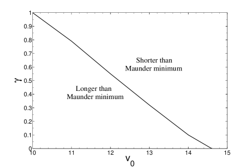
Figure 2: The parameter space indicating the reduction factor $\gamma$ of the poloidal field and the amplitude of the meridional circulation needed to produce Maunder-like grand minima.

Miyahara et al. (2004) found that cycles during the Maunder minimum became somewhat longer, indicating that the meridional circulation must have slowed down. This supports the theoretical idea that the weakening of meridional circulation might have played an important role in producing the Maunder minimum. It should be noted that the opposite would happen in the low diffusivity model. The weakening of meridional circulation and the lengthening of cycles in a low diffusivity model should be associated with a grand maximum, since longer cycles would allow the differential rotation to generate stronger fields in the low diffusivity model.

8 Concluding remarks

Although there are many uncertainties in our theoretical understanding of grand minima, it appears that fluctuations in poloidal field generation and fluctuations in meridional circulation are the main causes of irregularities in solar cycles and can also produce grand minima. We believe the solar dynamo to be a high diffusivity dynamo in which a fall in the meridional circulation makes cycles weaker. If fluctuations in poloidal field generation alone and fluctuations in meridional circulation alone are to produce grand minima, then the poloidal field at the end of a cycle or the meridional circulation has to fall to rather low values to cause grand minima. The situation is a little less constrained if we consider simultaneous fluctuations in both. Fig. 2 taken from Karak (2010) shows the values to which the poloidal field at the end of a cycle and the meridional circulation have to fall if a grand minimum is to be caused by their simultaneously falling to low values. This seems to be the most likely scenario we have at the present time for explaining grand minima. One important question is whether we can estimate how often this is likely to happen. Can we explain why there were 27 grand minima in the last 11,000 years? We are looking at this question right now.

I end by summarizing what appears to me to be the most plausible theoretical scenario for grand minima based on the flux transport dynamo. Due to fluctuations in poloidal field generation and meridional circulation, if both of them simultaneously happen to become sufficiently weak, that may push the Sun into a grand minimum. Within the grand minimum, the dynamo keeps operating on the basis of the $\alpha$-effect and ultimately bounces out of the grand minimum in the dynamo growth time.

References

- [Babcock (1961)] Babcock, H. W. 1961, ApJ, 133, 572
- [] Basu, S., & Antia, H. M. 2010, ApJ, 717, 488
- [] Beer, J., Tobias, S., & Weiss, N. 1998, Solar Phys., 181, 237
- [] Brandenburg, A., Krause, F., Meinel, R., Moss, D., & Tuominen I. 1989, A&A, 213, 411
- [] Brandenburg, A., & Spiegel, E. A. 2008, AN, 329, 351
- [] Charbonneau, P. 2005, Solar Phys., 229, 345
- [66] Charbonneau, P., Beaubien, G., & St-Jean, C. 2007, ApJ, 658, 657
- [] Charbonneau, P., Blais-Laurier, G., & St-Jean, C. 2004, ApJ, 616, L183
- [] Charbonneau, P., & Dikpati, M. 2000, ApJ, 543, 1027
- [65] Charbonneau, P., St-Jean, C., & Zacharias, P. 2005, ApJ, 619, 613
- [Chatterjee & Choudhuri (2006)] Chatterjee, P., & Choudhuri, A. R. 2006, Solar Phys., 239, 29
- [Chatterjee et al. (2004)] Chatterjee, P., Nandy, D., & Choudhuri, A. R. 2004, A&A, 427, 1019
- [Choudhuri (1989)] Choudhuri, A. R. 1989, Solar Phys., 123, 217
- [Choudhuri (1992)] Choudhuri, A. R. 1992, A&A, 253, 277
- [] Choudhuri, A. R. 1998, The Physics of Fluids and Plasmas: An Introduction for Astrophysicists (Cambridge University Press, Cambridge)
- [] Choudhuri, A. R. 2003, Solar Phys., 215, 31
- [Choudhuri et al. (2007)] Choudhuri, A. R., Chatterjee, P., & Jiang, J. 2007, Phys. Rev. Lett., 98, 131103
- [] Choudhuri A. R., & Gilman P.A. 1987, ApJ, 316, 788
- [Choudhuri & Karak (2009)] Choudhuri, A. R., & Karak, B. B. 2009, RAA, 9, 953
- [Choudhuri et al. (1995)] Choudhuri, A. R., Schüssler, M., & Dikpati, M. 1995, A&A, 303, L29
- [D’Silva & Choudhuri (1993)] D’Silva, S., & Choudhuri, A. R. 1993, A&A, 272, 621
- [] Fan, Y., Fisher, G. H., & DeLuca, E. E. 1993, ApJ, 405, 390
- [Goel & Choudhuri (2009)] Goel, A., & Choudhuri, A. R. 2009, RAA, 9, 115
- [] Guerrero, G., Dikpati, M., & de Gouveia Dal Pino, E. M. 2009 ApJ, 701, 725
- [] Hathaway, D. H., & Rightmire, L. 2010, Science, 327, 1350
- [Hotta & Yokoyama (2010)] Hotta, H., & Yokoyama, T. 2010, ApJ, 714, L308
- [] Hoyng, P. 1993, A&A, 272, 321
- [Hoyt & Schatten (1996)] Hoyt, D. V., & Schatten, K. H. 1996, Solar Phys., 165, 181
- [] Ivanova, T. S., & Ruzmaikin, A. A. 1977, SvA, 21, 479
- [Jiang et al. (2007)] Jiang, J., Chatterjee, P., & Choudhuri, A. R. 2007, MNRAS, 381, 1527
- [Karak (2010)] Karak, B. B. 2010, ApJ, 724, 1021
- [Karak & Choudhuri (2011)] Karak, B. B., & Choudhuri, A. R. 2011, MNRAS, 410, 1503
- [Karak & Choudhuri (2012)] Karak, B. B., & Choudhuri, A. R. 2012, Solar Phys., submitted (arXiv:1111.1540)
- [] Krause, F., & Meinel, R. 1988, GAFD, 43, 95
- [] Küker, M., Arlt, R., & Rüdiger, G. 1999, A&A 343, 977
- [Leighton (1969)] Leighton, R. B. 1969, ApJ, 156, 1
- [Longcope & Choudhuri (2002)] Longcope, D. W., & Choudhuri, A. R. 2002, Solar Phys., 205, 63
- [] Mininni, P. D., Gomez, D. O., & Mindlin, G. B. 2001, Solar Phys., 201, 203
- [] Miyahara, H., Masuda, K., Muraki, Y., Furuzawa, H., Menjo, H., & Nakamura, T. 2004, Solar Phys., 224, 317
- [] Moss, D., Brandenburg, A., Tavakol, R., & Tuominen, I. 1992, A&A, 265, 843
- [] Nandy, D., Muñoz-Jaramillo, A., & Martens, P. C. H. 2011 Nature 471, 80
- [] Ossendrijver, A. J. H., Hoyng, P., & Schmitt, D. 1996, A&A, 313, 938
- [Parker (1955)] Parker, E. N. 1955, ApJ, 122, 293
- [] Schmitt, D., & Schüssler, M. 1989, A&A, 223, 343
- [] Schmitt, D., Schüssler, M., & Ferriz-Mas, A. 1996, A&A, 311, L1
- [Sokoloff & Nesme-Ribes (1994)] Sokoloff, D., & Nesme-Ribes, E. 1994, A&A, 288, 293
- [Steenbeck et al. (1966)] Steenbeck, M., Krause, F., & Rädler, K. H. 1966, Z. Naturforsch., 21, 369
- [] Stix, M. 1972, A&A, 20, 9
- [] Usoskin, I. G., Mursula, K., & Kovaltsov, G. A. 2000, A&A, 354, L33
- [] Usoskin, I. G., Solanki, S. K., & Kovaltsov, G. A. 2007, A&A, 471, 301
- [] Vaquero, J. M., Gallego, M. C., Usoskin, I. G., & Kovaltsov, G. A. 2011, ApJ, 731, L24
- [] Weiss, N. O., Cattaaneo, F., & Jones, C. A. 1984, GAFD, 30, 305
- [Yeates et al. (2008)] Yeates, A. R., Nandy, D., & Mackay, D. H. 2008, ApJ, 673, 544
- [] Yoshimura, H. 1975, ApJ, 201, 740
- [] Yoshimura, H. 1978, ApJ, 226, 706