IPPP/11/70

DCPT/11/140

(incl. erratum)

Form Factors for $\Lambda_{b}\to\Lambda$ Transitions in SCET

Thorsten Feldmann, Matthew W Y Yip

IPPP, Department of Physics, University of Durham, Durham DH1 3LE, UK

We present a systematic discussion of $\Lambda_{b}\to\Lambda$ transition form factors in the framework of soft-collinear effective theory (SCET). The universal soft form factor, which enters the symmetry relations in the limit of large recoil energy, is calculated from a sum-rule analysis of a suitable SCET correlation function. The same method is applied to derive the leading corrections from hard-collinear gluon exchange at first order in the strong coupling constant. We present numerical estimates for form factors and form-factor ratios and their impact on decay observables in $\Lambda_{b}\to\Lambda\mu^{+}\mu^{-}$ decays.

1 Motivation

The decays $\Lambda_{b}\to\Lambda\ell^{+}\ell^{-}$ offer the possibility to study rare semi-leptonic and radiative $b\to s$ transitions within the Standard Model (SM) and beyond. The observables in the baryonic transitions provide complementary phenomenological information compared to the corresponding mesonic or inclusive decays, see e.g. [1, 2, 3, 4, 5, 6, 7, 8, 9]. The decay $\Lambda_{b}\to\Lambda\mu^{+}\mu^{-}$ has been recently measured by the CDF collaboration [10] with a branching ratio of the order $10^{-6}$.

Theoretical predictions for the exclusive decay matrix elements require non-perturbative hadronic input. To first approximation, this can be parametrized in terms of baryonic transition form factors for vector, axial-vector and tensor currents. The number of independent form factors drastically reduces in the limit of infinitely heavy $b$-quark mass, exploiting the approximate symmetries in heavy-quark effective theory (HQET), see e.g. [11, 12]. Additional simplification is expected in the kinematic limit of large recoil energy, $E_{\Lambda}\to\infty$, where the number of independent form factors is known to be reduced further [13], and part of the corrections to this limit should factorize in terms of process-independent hadronic quantities (light-cone distribution amplitudes, LCDAs, [15, 14]) and perturbative interaction kernels, in a similar way as it has been discussed for the analogous mesonic transitions [16]. The non-perturbative calculation of the remaining hadronic transition form factors can, for instance, be obtained from QCD sum rules. In the limit of large recoil energy, a systematic expansion in the heavy-quark mass is achieved in the framework of soft-collinear effective theory (SCET [17, 18]), where one studies the spectrum of correlation functions between the decay current and an interpolating current with the quantum numbers of the light hadron [19] (see also [20]).

The aim of this paper is to provide a systematic analysis of $\Lambda_{b}\to\Lambda$ form factors, starting from the symmetry relations in the heavy-quark/large-energy limit. To this end, in the next section, we will present a convenient definition of the 10 independent physical form factors, in terms of which the HQET and SCET symmetry relations look particularly simple. In the following section 3, we derive the leading expressions for the universal (“soft”) form factor $\xi_{\Lambda}$ from a sum-rule analysis of an appropriate correlation function in SCET, involving the LCDAs of the $\Lambda_{b}$ baryon. The same method is used to calculate the leading correction $\Delta\xi_{\Lambda}$ to the form-factor symmetry relations that arise from hard-collinear gluon exchange. In contrast to the mesonic case, one of the light spectator quarks still does not take part in the hard-scattering process, and therefore the corresponding effect could not be calculated in the framework of QCD factorization. (A similar discussion has been led for the electromagnetic form factors of the nucleon in [21].) The sum-rule expressions are analysed numerically in section 4. We focus on the theoretical uncertainty related to various hadronic input parameters entering the estimate for the soft form factor $\xi_{\Lambda}$. Part of these uncertainties drops out in the ratio $\Delta\xi_{\Lambda}/\xi_{\Lambda}$. We also provide estimates for the partial branching fractions (transverse and longitudinal rate, forward-backward asymmetry) of $\Lambda_{b}\to\Lambda\mu^{+}\mu^{-}$ in the large recoil (small $q^{2}$) limit, before we conclude. Finally, in our appendix, we collect the expressions for the double-differential $\Lambda_{b}\to\Lambda\mu^{+}\mu^{-}$ decay rates, and discuss an alternative form-factor basis that is optimized for a systematic discussion of power corrections to the symmetry relations. We also extract the hard vertex corrections to the $\Lambda_{b}\to\Lambda$ form factors arising from the matching of the decay currents from QCD onto SCET, and we identify 5 form-factor relations that are unaffected by short-distance ${\cal O}(\alpha_{s})$ corrections. Finally, we summarize the relevant information on baryon LCDAs and briefly comment on a simplified set-up with elementary light di-quark fields in the light and heavy baryon.

2 $\Lambda_{b}\to\Lambda$ Form Factors

In the following, we provide some useful definitions for $\Lambda_{b}\to\Lambda$ form factors that aim to improve previous definitions, as discussed for instance in [1, 4], in two aspects: (i) the form factors are defined from a helicity basis, (ii) the form factors are normalized to the limit of point-like hadrons. As a result, our form factor convention leads to rather simple expressions for partial rates, unitarity bounds (cf. [22, 23]) and symmetry relations in the HQET or SCET limit.

2.1 Helicity-Based Form-Factor Parametrization

The form factors for $\Lambda_{b}\to\Lambda$ transitions can be parametrized as follows. Starting with the vector and scalar decay currents, we have ($q=s(x)$ and $b=b(x)$ denote the light and heavy quark fields in the $b\to s$ transitions)

$$\langle\Lambda(p^{\prime},s^{\prime})|\bar{q}\,\gamma_{\mu}\,b|\Lambda_{b}(p,s)\rangle =\bar{u}_{\Lambda}(p^{\prime},s^{\prime})\left\{f_{0}(q^{2})\,(M_{\Lambda_{b}}-m_{\Lambda})\,\frac{q_{\mu}}{q^{2}}\right.$$ (2.1)

$$\qquad\left.+f_{+}(q^{2})\,\frac{M_{\Lambda_{b}}+m_{\Lambda}}{s_{+}}\,\left(p_{\mu}+p_{\mu}^{\prime}-\frac{q_{\mu}}{q^{2}}\,(M_{\Lambda_{b}}^{2}-m_{\Lambda}^{2})\right)\right.$$ (2.2)

$$\qquad\left.+f_{\perp}(q^{2})\left(\gamma_{\mu}-\frac{2m_{\Lambda}}{s_{+}}\,p_{\mu}-\frac{2M_{\Lambda_{b}}}{s_{+}}\,p^{\prime}_{\mu}\right)\right\}u_{\Lambda_{b}}(p,s)\,,$$ (2.3)

where we have defined

$$s_{\pm} =(M_{\Lambda_{b}}\pm m_{\Lambda})^{2}-q^{2}\,.$$ (2.4)

At vanishing momentum transfer, $q^{2}\to 0$, one further has the kinematic constraint

$$f_{0}(0) =f_{+}(0)\,.$$ (2.5)

The individual form factors are defined in such a way that they correspond to time-like (scalar), longitudinal and transverse polarization with respect to the momentum-transfer $q^{\mu}$ for $f_{0}$, $f_{+}$ and $f_{\perp}$, respectively (cf. [22, 23]). The normalization is chosen in such a way that for

$$f_{0},f_{+},f_{\perp}\to 1\,,$$

one recovers the expression for a transition between point-like baryons, i.e. $\langle\Lambda|\bar{q}\,\Gamma\,b|\Lambda_{b}\rangle\to\bar{u}_{\Lambda}\,\Gamma\,u_{\Lambda_{b}}$. The form factor $f_{0}$ is also obtained from the scalar decay current via the equations of motion (e.o.m.),

$$\langle\Lambda(p^{\prime},s^{\prime})|\bar{q}\,b|\Lambda_{b}(p,s)\rangle =\frac{q^{\mu}}{M_{b}-m_{q}}\,\langle\Lambda(p^{\prime},s^{\prime})|\bar{q}\,\gamma_{\mu}\,b|\Lambda_{b}(p,s)\rangle$$ (2.6)

$$=f_{0}(q^{2})\,\frac{M_{\Lambda_{b}}-m_{\Lambda}}{M_{b}-m_{q}}\,\bar{u}_{\Lambda}(p^{\prime},s^{\prime})\,u_{\Lambda_{b}}(p,s)\,.$$ (2.7)

The expression for the axial-vector and pseudo-scalar currents can be obtained by appropriately changing the relative sign between the light and heavy baryon mass, and we thus define

$$\langle\Lambda(p^{\prime},s^{\prime})|\bar{q}\,\gamma_{\mu}\gamma_{5}\,b|\Lambda_{b}(p,s)\rangle ={}-\bar{u}_{\Lambda}(p^{\prime},s^{\prime})\gamma_{5}\left\{g_{0}(q^{2})\,(M_{\Lambda_{b}}+m_{\Lambda})\,\frac{q_{\mu}}{q^{2}}\right.$$ (2.8)

$$\qquad\left.+g_{+}(q^{2})\,\frac{M_{\Lambda_{b}}-m_{\Lambda}}{s_{-}}\left(p_{\mu}+p_{\mu}^{\prime}-\frac{q_{\mu}}{q^{2}}\,(M_{\Lambda_{b}}^{2}-m_{\Lambda}^{2})\right)\right.$$ (2.9)

$$\qquad\left.+g_{\perp}(q^{2})\left(\gamma_{\mu}+\frac{2m_{\Lambda}}{s_{-}}\,p_{\mu}-\frac{2M_{\Lambda_{b}}}{s_{-}}\,p^{\prime}_{\mu}\right)\right\}u_{\Lambda_{b}}(p,s)\,,$$ (2.10)

with the kinematic constraint $g_{0}(0)=g_{+}(0)$ at $q^{2}\to 0$, and

$$\langle\Lambda(p^{\prime},s^{\prime})|\bar{q}\,\gamma_{5}\,b|\Lambda_{b}(p,s)\rangle =\frac{q^{\mu}}{M_{b}+m_{q}}\,\langle\Lambda(p^{\prime},s^{\prime})|\bar{q}\,\gamma_{5}\gamma_{\mu}\,b|\Lambda_{b}(p,s)\rangle$$ (2.12)

$$=g_{0}(q^{2})\,\frac{M_{\Lambda_{b}}+m_{\Lambda}}{M_{b}+m_{q}}\,\bar{u}_{\Lambda}(p^{\prime},s^{\prime})\,\gamma_{5}u_{\Lambda_{b}}(p,s)\,.$$ (2.13)

Finally, for the tensor and pseudo-tensor current, we write

$$\langle\Lambda(p^{\prime},s^{\prime})|\bar{q}\,i\sigma_{\mu\nu}q^{\nu}\,b|\Lambda_{b}(p,s)\rangle$$ (2.14)

$$={}-\bar{u}_{\Lambda}(p^{\prime},s^{\prime})\left\{h_{+}(q^{2})\,\frac{q^{2}}{s_{+}}\left(p_{\mu}+p_{\mu}^{\prime}-\frac{q_{\mu}}{q^{2}}\,(M_{\Lambda_{b}}^{2}-m_{\Lambda}^{2})\right)\right.$$ (2.15)

$$\qquad\left.+(M_{\Lambda_{b}}+m_{\Lambda})\,h_{\perp}(q^{2})\left(\gamma_{\mu}-\frac{2m_{\Lambda}}{s_{+}}\,p_{\mu}-\frac{2M_{\Lambda_{b}}}{s_{+}}\,p^{\prime}_{\mu}\right)\right\}u_{\Lambda_{b}}(p,s)\,,$$ (2.16)

and

$$\langle\Lambda(p^{\prime},s^{\prime})|\bar{q}\,i\sigma_{\mu\nu}\gamma_{5}q^{\nu}\,b|\Lambda_{b}(p,s)\rangle$$ (2.17)

$$={}-\bar{u}_{\Lambda}(p^{\prime},s^{\prime})\gamma_{5}\left\{\tilde{h}_{+}(q^{2})\,\frac{q^{2}}{s_{-}}\left(p_{\mu}+p_{\mu}^{\prime}-\frac{q_{\mu}}{q^{2}}\,(M_{\Lambda_{b}}^{2}-m_{\Lambda}^{2})\right)\right.$$ (2.18)

$$\qquad\left.+(M_{\Lambda_{b}}-m_{\Lambda})\,\tilde{h}_{\perp}(q^{2})\left(\gamma_{\mu}+\frac{2m_{\Lambda}}{s_{-}}\,p_{\mu}-\frac{2M_{\Lambda_{b}}}{s_{-}}\,p^{\prime}_{\mu}\right)\right\}u_{\Lambda_{b}}(p,s)\,.$$ (2.19)

Again, the normalization of the form factors $h_{\perp,+},\tilde{h}_{\perp,+}$ has been fixed by the case of point-like hadrons. This makes 10 independent form factors for the general case, after the e.o.m. have been taken into account. In terms of the helicity form factors, the differential decay width for $\Lambda_{b}\to\Lambda\mu^{+}\mu^{-}$ takes a particularly simple form, see Appendix A. An alternative parametrization, which is based on the large and small projections of energetic or massive fermion spinors, can be found in Appendix B.2.

2.2 HQET Limit

The number of independent $\Lambda_{b}\to\Lambda$ form factors reduces considerably in the heavy quark limit, $M_{b}\to\infty$ (see e.g. [12]), when we use the heavy-baryon velocity $v^{\mu}$ to project onto the large spinor components $h_{v}^{(b)}=\hbox to0.0pt{\hbox to5.20601pt{\hfil/\hfil}\hss}v\,h_{v}^{(b)}$ of the heavy $b$-quark field,

$$\langle\Lambda(p^{\prime},s^{\prime})|\bar{q}\,\Gamma\,b|\Lambda_{b}(p,s)\rangle \to\langle\Lambda(p^{\prime},s^{\prime})|\bar{q}\,\Gamma\,h_{v}^{(b)}|\Lambda_{b}(v,s)\rangle$$ (2.20)

$$\simeq\bar{u}_{\Lambda}(p^{\prime},s^{\prime})\left(A(v\cdot p^{\prime})+\hbox to0.0pt{\hbox to5.20601pt{\hfil/\hfil}\hss}v\,B(v\cdot p^{\prime})\right)\Gamma\,u_{\Lambda_{b}}(v,s)\,.$$ (2.21)

Here $\Gamma$ is an arbitrary Dirac matrix, and $p^{\mu}=M_{\Lambda_{b}}v^{\mu}\simeq M_{b}v^{\mu}$. Furthermore, $|\Lambda_{b}(v,s)\rangle$ is a heavy-baryon state, and $u_{\Lambda_{b}}(v,s)=\hbox to0.0pt{\hbox to5.20601pt{\hfil/\hfil}\hss}v\,u_{\Lambda_{b}}(v,s)$ a heavy-baryon spinor in HQET. In the heavy-quark limit, $m_{\Lambda},v\cdot p^{\prime}\ll M_{b}$, the helicity form factors are related to the two HQET form factors in (2.21) as follows,

$$\mbox{\text@underline{small recoil:}}\quad\ f_{0}(q^{2})\simeq g_{+}(q^{2})\simeq g_{\perp}(q^{2})\simeq\tilde{h}_{+}(q^{2})\simeq\tilde{h}_{\perp}(q^{2})\simeq \ A(v\cdot p^{\prime})+B(v\cdot p^{\prime})\,,$$ (2.22)

$$g_{0}(q^{2})\simeq f_{+}(q^{2})\simeq f_{\perp}(q^{2})\simeq h_{+}(q^{2})\simeq h_{\perp}(q^{2})\simeq \ A(v\cdot p^{\prime})-B(v\cdot p^{\prime})\,,$$ (2.23)

with $q^{2}=M_{\Lambda_{b}}^{2}-2M_{\Lambda_{b}}\,v\cdot p^{\prime}+m_{\Lambda}^{2}$.

2.3 SCET Limit and Hard-Scattering Corrections

In the kinematic region of large recoil energy for the $\Lambda$ baryon in the rest frame of the decaying $\Lambda_{b}$, further simplifications arise [13, 16]. A formal derivation can be obtained from soft-collinear effective theory (SCET) [17, 18]. To this end, we consider the matrix element of the leading current involving the collinear quark field $\xi\equiv\frac{\hbox to0.0pt{\hbox to4.20164pt{\hfil/\hfil}\hss}n_{-}\hbox to0.0pt{\hbox to4.20164pt{\hfil/\hfil}\hss}n_{+}}{4}\,q$ with two light-like vectors $n_{-}^{2}=n_{+}^{2}=0$, satisfying $(n_{+}+n_{-})/2=v$ and $n_{-}\cdot n_{+}=2$. In the large-energy limit, we can further set $p^{\prime}{}^{\mu}\simeq(n_{+}p^{\prime})n_{-}^{\mu}/2$ and $m_{\Lambda}\to 0$. This amounts to

$$\langle\Lambda(p^{\prime},s^{\prime})|\bar{\xi}W\,\Gamma\,Y^{\dagger}h_{v}^{(b)}|\Lambda_{b}(v,s)\rangle=\bar{u}_{\Lambda}(p^{\prime},s^{\prime})\left(A(q^{2})+\hbox to0.0pt{\hbox to5.20601pt{\hfil/\hfil}\hss}v\,B(q^{2})\right)\frac{\hbox to0.0pt{\hbox to6.00235pt{\hfil/\hfil}\hss}n_{+}\hbox to0.0pt{\hbox to6.00235pt{\hfil/\hfil}\hss}n_{-}}{4}\,\Gamma\,u_{\Lambda_{b}}(v,s)$$ (2.24)

$$\qquad=A(q^{2})\,\bar{u}_{\Lambda}(p^{\prime},s^{\prime})\,\frac{\hbox to0.0pt{\hbox to6.00235pt{\hfil/\hfil}\hss}n_{+}\hbox to0.0pt{\hbox to6.00235pt{\hfil/\hfil}\hss}n_{-}}{4}\,\Gamma\,u_{\Lambda_{b}}(v,s)+B(q^{2})\,\bar{u}_{\Lambda}(p^{\prime},s^{\prime})\,\frac{\hbox to0.0pt{\hbox to6.00235pt{\hfil/\hfil}\hss}n_{-}}{2}\,\Gamma\,u_{\Lambda_{b}}(v,s)\,.$$ (2.25)

Here $W$ ($Y$) are Wilson lines in SCET that render the definition of the form factors invariant under collinear (soft) gauge transformations. In the following, we will always drop the Wilson lines (which corresponds to light-cone gauges for collinear and soft gluon fields). Exploiting the (approximate) equations of motion for $\bar{u}_{\Lambda}(p^{\prime},s^{\prime})\,\hbox to0.0pt{\hbox to6.00235pt{\hfil/\hfil}\hss}n_{-}\simeq 0$, this simplifies to

$$\langle\Lambda(p^{\prime},s^{\prime})|\bar{\xi}\,\Gamma\,h_{v}^{(b)}|\Lambda_{b}(v,s)\rangle\simeq\xi_{\Lambda}(n_{+}p^{\prime})\,\bar{u}_{\Lambda}(p^{\prime},s^{\prime})\,\Gamma\,u_{\Lambda_{b}}(v,s)\,,$$ (2.26)

where $\xi_{\Lambda}(n_{+}p^{\prime})$ corresponds to $A(v\cdot p^{\prime})$ in (2.23) and defines the so-called “soft” $\Lambda_{b}\to\Lambda$ form factor, while the contribution from $B(v\cdot p^{\prime})$ is negligible. In the SCET limit, $n_{+}p^{\prime}\sim M_{\Lambda_{b}}$, all helicity form factors are thus equal to $\xi_{\Lambda}(n_{+}p^{\prime})$,

large recoil: $$f_{0}(q^{2})\approx f_{+}(q^{2})\approx f_{\perp}(q^{2})\approx h_{+}(q^{2})\approx h_{\perp}(q^{2})$$ (2.27)

$$\approx\ g_{0}(q^{2})\approx g_{+}(q^{2})\approx g_{\perp}(q^{2})\approx\tilde{h}_{+}(q^{2})\approx\tilde{h}_{\perp}(q^{2})\ \approx\ \xi_{\Lambda}(n_{+}p^{\prime})\,,$$ (2.28)

with $q^{2}=M_{\Lambda_{b}}^{2}-M_{\Lambda_{b}}\,n_{+}p^{\prime}+m_{\Lambda}^{2}\left(1-\frac{M_{\Lambda_{b}}}{n_{+}p^{\prime}}\right)$.

The leading corrections to the form factor relations from hard-collinear gluon exchange can be described by a form factor term that takes into account the corresponding sub-leading currents in SCET, which contain one additional (transverse) hard-collinear gluon field [18]. If we neglect additional hard vertex corrections for simplicity, the form factors relate to matrix elements of local SCET currents. In the limit $M_{b}\to\infty$, $(n_{+}p^{\prime})\to\infty$, these matrix element can again be described by a single form factor $\Delta\xi_{\Lambda}$, which we define by

$$\langle\Lambda(p^{\prime},s^{\prime})|\bar{\xi}\,\tilde{\Gamma}\,gA_{\mu}^{\perp}\,h_{v}^{(b)}|\Lambda_{b}(v,s)\rangle \equiv M_{\Lambda_{b}}\,\Delta\xi_{\Lambda}(n_{+}p^{\prime})\ \bar{u}_{\Lambda}(p^{\prime},s^{\prime})\,\gamma_{\mu}^{\perp}\,\tilde{\Gamma}\,u_{\Lambda_{b}}(v,s)\,,$$ (2.29)

where the basis of independent Dirac matrices can be reduced to $\tilde{\Gamma}=\frac{\hbox to0.0pt{\hbox to4.20164pt{\hfil/\hfil}\hss}n_{+}}{2}\,\{1,\gamma_{\nu}^{\perp},\gamma_{5}\}$. Here we have exploited again that, due to the heavy-quark spin symmetry, the Dirac matrix in the effective-theory decay current couples trivially to the heavy baryon spinor. The matching of the various decay currents in QCD onto the SCET currents is process-independent and can be taken into account by appropriate Wilson coefficients. For convenience, we have summarized the relevant results in Appendix C.

3 Sum rules in SCET

Our next aim is to obtain non-perturbative estimates for the form factors $\xi_{\Lambda}$ and $\Delta\xi_{\Lambda}$ in the large-recoil limit, following the analogous calculation as for the $B\to\pi(\rho)$ form factors from SCET sum rules in [19]. The leading diagrams for the calculation of the respective correlation functions are shown in Fig. 1.

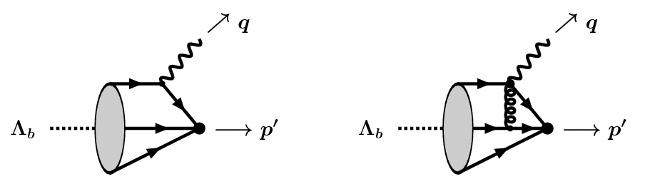
Figure 1: Leading diagrams for SCET correlation functions involving the soft form factor $\xi_{\Lambda}$ (left) and the form factor $\Delta\xi_{\Lambda}$ for the hard-scattering corrections in the large-recoil limit.

3.1 Soft form factor

We start with a correlation function, where the $\Lambda$ baryon in the final state is replaced by an interpolating current sharing the same quantum numbers. We choose

$$J_{\Lambda}(x) \equiv\epsilon^{abc}\left(u^{a}(x)\,C\,\gamma_{5}\hbox to0.0pt{\hbox to6.00235pt{\hfil/\hfil}\hss}n_{+}\,d^{b}(x)\right)s^{c}(x)\,,$$ (3.30)

which is normalized by the matrix element

$$\langle 0|\frac{\hbox to0.0pt{\hbox to6.00235pt{\hfil/\hfil}\hss}n_{\mp}\hbox to0.0pt{\hbox to6.00235pt{\hfil/\hfil}\hss}n_{\pm}}{4}\,J_{\Lambda}(0)|\Lambda(p^{\prime},s^{\prime})\rangle =(n_{+}p^{\prime})\,f_{\Lambda}\,\frac{\hbox to0.0pt{\hbox to6.00235pt{\hfil/\hfil}\hss}n_{\mp}\hbox to0.0pt{\hbox to6.00235pt{\hfil/\hfil}\hss}n_{\pm}}{4}\,u_{\Lambda}(p^{\prime},s^{\prime})\,,$$ (3.31)

and thus corresponds to a leading term in the large-energy limit. A sum-rule estimate [15] gives $f_{\Lambda}\simeq(6.0\pm 0.3)\times 10^{-3}~{}{\rm GeV}^{2}$ for the involved decay constant of the $\Lambda$ baryon (for comparison, for the nucleon $f_{N}\simeq 5.6\times 10^{-3}~{}{\rm GeV}^{2}$ has been estimated in [24]). The various light-quark fields can be decomposed into soft and hard-collinear fields to match the above current onto SCET. At tree-level, it is sufficient to calculate the correlation function in QCD and perform the appropriate kinematic limits for the propagators.

We now define the correlation function between a weak decay current and the interpolating current $J_{\Lambda}$, and consider it as a function of the small (Euclidean) momentum component $(n_{-}p^{\prime})<0$ for $p_{\perp}^{\prime}\equiv 0$ and fixed large momentum component $(n_{+}p^{\prime})$. In order to extract the universal soft form factor $\xi_{\Lambda}$, we consider the projection of a decay current on the large spinor components for the light and heavy quark fields. We therefore have

$$\Pi_{\Lambda}(n_{-}p^{\prime}) \equiv i\int d^{4}x\,e^{ip^{\prime}x}\langle 0|T\left[\frac{\hbox to0.0pt{\hbox to6.00235pt{\hfil/\hfil}\hss}n_{-}\hbox to0.0pt{\hbox to6.00235pt{\hfil/\hfil}\hss}n_{+}}{4}\,J_{\Lambda}(x)\left[\bar{s}(0)\,\frac{\hbox to0.0pt{\hbox to6.00235pt{\hfil/\hfil}\hss}n_{+}\hbox to0.0pt{\hbox to6.00235pt{\hfil/\hfil}\hss}n_{-}}{4}\,\Gamma\,\frac{1+\hbox to0.0pt{\hbox to5.20601pt{\hfil/\hfil}\hss}v}{2}\,b(0)\right]\right]|\Lambda_{b}(p)\rangle\,.$$ (3.32)

The time-ordered product of the two currents can be calculated in perturbation theory. The leading diagram just corresponds to the one shown on the left-hand side in Fig. 1, which refers to the situation where the two strange-quark fields are contracted to a propagator, while the up- and down-quark merely act as spectators. Employing the kinematic limits in the QCD diagram, and performing a Fourier transform such that $\omega_{1,2}=(n_{-}k_{1,2})$ correspond to the light-cone momenta of the up- and down-quark, the correlation function at leading order is given by

$$\Pi_{\Lambda}(n_{-}p^{\prime}) \simeq\int\frac{d\omega_{1}\,d\omega_{2}}{\omega_{1}+\omega_{2}-n_{-}p^{\prime}-i\epsilon}\,\langle 0|\epsilon^{abc}\left(u^{a}(\omega_{1})\,C\,\gamma_{5}\hbox to0.0pt{\hbox to6.00235pt{\hfil/\hfil}\hss}n_{+}\,d^{b}(\omega_{2})\right)\frac{\hbox to0.0pt{\hbox to6.00235pt{\hfil/\hfil}\hss}n_{-}}{2}\,\Gamma\,b^{c}_{v}|\Lambda_{b}(v,s)\rangle$$ (3.33)

$$=f_{\Lambda_{b}}^{(2)}\int\frac{d\omega_{1}\,d\omega_{2}\,\psi_{4}(\omega_{1},\omega_{2})}{\omega_{1}+\omega_{2}-n_{-}p^{\prime}-i\epsilon}\ \frac{\hbox to0.0pt{\hbox to6.00235pt{\hfil/\hfil}\hss}n_{-}}{2}\,\Gamma\,u_{\Lambda_{b}}(v,s)$$ (3.34)

$$=f_{\Lambda_{b}}^{(2)}\int_{0}^{\infty}\frac{d\omega\,\omega\,\int_{0}^{1}du\,\tilde{\psi}_{4}(\omega,u)}{\omega-n_{-}p^{\prime}-i\epsilon}\ \frac{\hbox to0.0pt{\hbox to6.00235pt{\hfil/\hfil}\hss}n_{-}}{2}\,\Gamma\,u_{\Lambda_{b}}(v,s)\,.$$ (3.35)

To arrive at the second and third line, we have used the momentum-space projector for the heavy $\Lambda_{b}$ baryon, following from the definition of its light-cone distribution amplitudes as derived in Appendix D. To leading order, the result for the correlation function thus only involves the sum of the spectator-quark momenta and therefore only requires the partially integrated LCDA

$$\phi_{4}(\omega)\equiv\omega\int_{0}^{1}du\,\tilde{\psi}_{4}(\omega,u)\,.$$

The remaining analysis is then very similar to the $B\to\pi,\rho$ case discussed in [19]. For the hadronic side of the sum rule, the contribution of the $\Lambda$ baryon to the correlator is given by

$$\Pi_{\Lambda}\big{|}_{\rm res.} \simeq\sum_{s^{\prime}}\frac{\hbox to0.0pt{\hbox to6.00235pt{\hfil/\hfil}\hss}n_{-}\hbox to0.0pt{\hbox to6.00235pt{\hfil/\hfil}\hss}n_{+}}{4}\,\frac{\langle 0|J_{\Lambda}|\Lambda(p^{\prime},s^{\prime})\rangle\langle\Lambda(p^{\prime},s^{\prime})|\bar{q}\,\frac{\hbox to0.0pt{\hbox to4.20164pt{\hfil/\hfil}\hss}n_{+}\hbox to0.0pt{\hbox to4.20164pt{\hfil/\hfil}\hss}n_{-}}{4}\,\Gamma\,h_{v}^{(b)}|\Lambda_{b}(v)\rangle}{m_{\Lambda}^{2}-(p^{\prime})^{2}}$$ (3.36)

$$=\frac{(n_{+}p^{\prime})\,f_{\Lambda}\,\xi_{\Lambda}(n_{+}p^{\prime})}{m_{\Lambda}^{2}-(n_{+}p^{\prime})(n_{-}p^{\prime})}\,\sum_{s^{\prime}}\frac{\hbox to0.0pt{\hbox to6.00235pt{\hfil/\hfil}\hss}n_{-}\hbox to0.0pt{\hbox to6.00235pt{\hfil/\hfil}\hss}n_{+}}{4}\,u_{\Lambda}(p^{\prime},s^{\prime})\,\bar{u}_{\Lambda}(p^{\prime},s^{\prime})\,\frac{\hbox to0.0pt{\hbox to6.00235pt{\hfil/\hfil}\hss}n_{+}\hbox to0.0pt{\hbox to6.00235pt{\hfil/\hfil}\hss}n_{-}}{4}\,\Gamma\,u_{\Lambda_{b}}(v,s)$$ (3.37)

$$=\frac{(n_{+}p^{\prime})\,f_{\Lambda}\,\xi_{\Lambda}(n_{+}p^{\prime})}{m_{\Lambda}^{2}/(n_{+}p^{\prime})-(n_{-}p^{\prime})}\,\frac{\hbox to0.0pt{\hbox to6.00235pt{\hfil/\hfil}\hss}n_{-}}{2}\,\Gamma\,u_{\Lambda_{b}}(v,s)\,.$$ (3.38)

Comparing the perturbative and hadronic parts of the sum rule, subtracting the continuum (which is modelled by the perturbative result above a threshold parameter $\omega_{s}$), and performing a Borel transformation in terms of the Borel parameter $\omega_{M}$, we obtain the LO sum rule

$$e^{-m_{\Lambda}^{2}/(n_{+}p^{\prime})\omega_{M}}\,(n_{+}p^{\prime})\,f_{\Lambda}\,\xi_{\Lambda}(n_{+}p^{\prime}) =f_{\Lambda_{b}}^{(2)}\int_{0}^{\omega_{s}}d\omega\,\phi_{4}(\omega)\,e^{-\omega/\omega_{M}}\,,$$ (3.39)

which takes the analogous form as for the $B\to\pi,\rho$ case, only that the distribution amplitude for the spectator anti-quark in the $B$-meson is replaced by the effective LCDA for the spectator di-quark in the $\Lambda_{b}$ baryon.

The formal scaling of the (tree-level) result for $\xi_{\Lambda}$ with the large-energy variable can be derived by further considering the limit $\omega_{s,M}\sim\frac{\Lambda_{\rm had.}^{2}}{n_{+}p^{\prime}}\ll\langle\omega\rangle$, which allows one to expand the LCDA of the $\Lambda_{b}$ baryon around $\omega=0$ in the integrand. This yields

$$\xi_{\Lambda}(n_{+}p^{\prime}) \approx\frac{f_{\Lambda_{b}}^{(2)}\,\omega_{M}^{2}\,\phi_{4}^{\prime}(0)}{(n_{+}p^{\prime})\,f_{\Lambda}}\,e^{m_{\Lambda}^{2}/(n_{+}p^{\prime})\omega_{M}}\left(1-e^{-\omega_{s}/\omega_{M}}\,(1+\frac{\omega_{s}}{\omega_{M}})\right)\,.$$ (3.40)

where $\phi_{4}^{\prime}(0)\sim 1/\omega_{0}^{2}$ with $\omega_{0}\sim\langle\omega\rangle$ being the typical light-come momentum of the light di-quark in the heavy baryon (see Appendix D). In this limit, the soft $\Lambda_{b}\to\Lambda$ form factor thus scales as $1/(n_{+}p^{\prime})^{3}$ with the large energy of the final state baryon. Compared to the mesonic case [19], one encounters an additional factor of $1/(n_{+}p^{\prime})$ which physically can be traced back to the phase-space suppression of the additional spectator quark. Technically, the difference between the mesonic and baryonic case stems from the fact that the B-meson LCDA $\phi_{B}^{-}(\omega)$ does not vanish at the endpoint, while $\phi_{4}(\omega)$ vanishes linearly.

We should stress that radiative corrections to the sum rule will lead to additional non-analytical dependence of the form factors on $(n_{+}p^{\prime})$ with logarithmically enhanced perturbative coefficients. Part of these corrections are universal and can be uniquely factorized in terms of: (i) hard vertex corrections absorbed in Wilson coefficients of SCET decay currents, (ii) a jet function, absorbing the hard-collinear emissions from the strange-quark propagator in SCET, (iii) the soft evolution of the LCDAs of the $\Lambda_{b}$ baryon. To this accuracy, we obtain an analogous result as discussed for the mesonic case [19],

$$F_{i}(q^{2}) \simeq C_{i}(n_{+}p^{\prime},\mu)\cdot\frac{e^{m_{\Lambda}^{2}/(n_{+}p^{\prime})\omega_{M}}\,f_{\Lambda_{b}}^{(2)}}{(n_{+}p^{\prime})\,f_{\Lambda}}\int_{0}^{\omega_{s}}d\omega^{\prime}\,e^{-\omega^{\prime}/\omega_{M}}$$ (3.41)

$$\quad\Bigg{\{}\left[1+\frac{\alpha_{s}C_{F}}{4\pi}\left(7-\pi^{2}+3\ln\left[\frac{\mu^{2}}{\omega^{\prime}(n_{+}p^{\prime})}\right]+2\ln^{2}\left[\frac{\mu^{2}}{\omega^{\prime}(n_{+}p^{\prime})}\right]\right)\right]\phi_{4}(\omega^{\prime},\mu)$$ (3.42)

$$\quad{}+\frac{\alpha_{s}C_{F}}{4\pi}\,\int\limits_{0}^{\omega^{\prime}}d\omega\left(4\ln\left[\frac{\mu^{2}}{(\omega^{\prime}-\omega)(n_{+}p^{\prime})}\right]+3\right)\,\frac{\phi_{4}(\omega^{\prime},\mu)-\phi_{4}(\omega,\mu)}{\omega^{\prime}-\omega}\Bigg{\}}\,,$$ (3.43)

where $F_{i}(q^{2})$ denotes a generic form factor with the corresponding Wilson coefficient $C_{i}$. The leading (double-logarithmic) $\mu$-dependence cancels between the 3 terms on the right-hand side, thanks to the renormalization-group equations (see e.g. [17, 14, 25, 26, 27]),

$$\frac{d}{d\ln\mu}\,C_{i}(n_{+}p^{\prime},\mu) =-\frac{\alpha_{s}C_{F}}{4\pi}\,\Gamma_{\rm cusp}^{(1)}\,\ln\frac{\mu}{M_{b}}\,C_{i}(n_{+}p^{\prime},\mu)+\ldots\,,$$ (3.44)

$$\frac{d}{d\ln\mu}\,\phi_{4}(\omega,\mu) =-\frac{\alpha_{s}C_{F}}{4\pi}\,\Gamma_{\rm cusp}^{(1)}\,\ln\frac{\mu}{\omega}\,\phi_{4}(\omega,\mu)+\ldots$$ (3.45)

with the cusp-anomalous dimension $\Gamma_{\rm cusp}^{(1)}=4$. Evaluating the terms in curly brackets in (3.43) at a factorization scale of order $\mu^{2}\sim\omega_{s}(n_{+}p^{\prime})$ and evolving the Wilson coefficients down to that scale, one achieves the resummation of the leading Sudakov double logarithms.

Additional process-dependent corrections to (3.43) arise from hard-collinear gluon exchange between the strange quark and the spectator quarks in SCET. As shown in [19], these will lead to logarithmically enhanced terms which are sensitive to the endpoint behaviour of $\phi_{4}(\omega,\mu)$. The explicit derivation of these terms is left for future work.

3.2 Corrections from Hard-Collinear Gluon Exchange

As explained above, sub-leading currents in the SCET Lagrangian will induce violations of the form-factor symmetry relations in the large recoil limit. Contributions involving hard-collinear gluon exchange can be treated perturbatively in SCET correlation functions. The leading effect requires one to calculate the matrix element in (2.29), whose leading contribution arises from hard-collinear gluon exchange with one of the two spectator quarks in the baryons, see the corresponding diagram on the r.h.s. of Fig. 1. From the perspective of QCD factorization, this diagram represents an intermediate (hybrid) case, where some of the constituents undergo calculable short-distance interactions, while the remaining spectator quark remains undisturbed and is thus forced to populate the endpoint region in phase space.

In the sum-rule approach, as before, we define a correlation function (in light-cone gauge)

$$\Pi_{\Lambda}^{\mu}(n_{-}p^{\prime}) \equiv i\int d^{4}x\,e^{ip^{\prime}x}\langle 0|T\left[\frac{\hbox to0.0pt{\hbox to6.00235pt{\hfil/\hfil}\hss}n_{+}\hbox to0.0pt{\hbox to6.00235pt{\hfil/\hfil}\hss}n_{-}}{4}\,J_{\Lambda}(x)\left[\bar{s}(0)\,\tilde{\Gamma}\,gA^{\mu}_{\perp}(0)\,b(0)\right]\right]|\Lambda_{b}(p)\rangle\,.$$ (3.46)

Notice that this time, we have to use the opposite light-cone projector acting on $J_{\Lambda}$, as compared to the correlation function used to extract the soft form factor $\xi_{\Lambda}$. It projects on the sub-leading transverse momentum in the numerator of the strange-quark propagator which is required from rotational invariance in the transverse plane. The light-quark momenta in the $\Lambda_{b}$ baryon again are denoted as $k_{1,2}$ respectively, with $k_{1}=\omega_{1}+k_{1\perp}$, $k_{2}=\omega_{2}+k_{2\perp}$, and $\omega=\omega_{1}+\omega_{2}=n_{-}k$. Using the momentum-space projector for the LCDAs of $\Lambda_{b}$ as given in Appendix D, and assuming isospin symmetry of strong interactions, we obtain

$$\Pi^{\mu}(n_{-}p^{\prime})=-i\,g_{s}^{2}\,C_{F}\,\frac{f_{\Lambda_{b}}^{(2)}}{4}\,\int d\omega_{1}\int d\omega_{2}$$ (3.47)

$$\quad\times\int\frac{d^{D}l}{(2\pi)^{D}}\,\frac{1}{[l_{\perp}^{2}+(n_{+}l)(n_{-}l)][l_{\perp}^{2}+(n_{+}l)\,(n_{-}l-\omega_{2})][l_{\perp}^{2}+(n_{+}p^{\prime}+n_{+}l)(n_{-}p^{\prime}+n_{-}l-\omega)]}$$ (3.48)

$$\quad\times{\rm tr}\left[\tilde{M}(k_{1},k_{2})\,C\gamma_{5}\hbox to0.0pt{\hbox to6.00235pt{\hfil/\hfil}\hss}n_{+}(\hbox to0.0pt{\hbox to5.52084pt{\hfil/\hfil}\hss}k_{2}-\hbox to0.0pt{\hbox to5.00002pt{\hfil$l$\hfil}\hss}/)\gamma^{\mu}_{\perp}\right]\frac{\hbox to0.0pt{\hbox to6.00235pt{\hfil/\hfil}\hss}n_{+}\hbox to0.0pt{\hbox to6.00235pt{\hfil/\hfil}\hss}n_{-}}{4}\,(\hbox to0.0pt{\hbox to5.00002pt{\hfil$l$\hfil}\hss}/-\hbox to0.0pt{\hbox to5.52084pt{\hfil/\hfil}\hss}k_{1}-\hbox to0.0pt{\hbox to5.52084pt{\hfil/\hfil}\hss}k_{2})\,\tilde{\Gamma}\,u_{\Lambda_{b}}(v,s)\,,$$ (3.49)

where the square bracket around propagator denominators imply a “$+i\epsilon$” description. The Dirac trace is easily calculated as

$${\rm tr}\left[\tilde{M}(k_{1},k_{2})\,C\gamma_{5}\hbox to0.0pt{\hbox to6.00235pt{\hfil/\hfil}\hss}n_{+}(\hbox to0.0pt{\hbox to5.52084pt{\hfil/\hfil}\hss}k_{2}-\hbox to0.0pt{\hbox to5.00002pt{\hfil$l$\hfil}\hss}/)\gamma^{\mu}_{\perp}\right]$$ (3.50)

$$\quad=-4\psi_{4}(\omega_{1},\omega_{2})\,l_{\perp}^{\mu}+2(n_{+}l)\left(G(\omega_{1},\omega_{2})\,\frac{\partial}{\partial k_{1\mu}^{\perp}}+H(\omega_{1},\omega_{2})\,\frac{\partial}{\partial k_{2\mu}^{\perp}}\right)\,.$$ (3.51)

This yields

$$\Pi^{\mu}(n_{-}p^{\prime})=i\,\frac{g_{s}^{2}C_{F}f_{\Lambda_{b}}^{(2)}}{2}\,\int d\omega_{1}\int d\omega_{2}$$ (3.52)

$$\quad\times\int\frac{d^{D}l}{(2\pi)^{D}}\,\frac{2l_{\perp}^{2}/(D-2)\,\psi_{4}(\omega_{1},\omega_{2})+(n_{+}l)\left(G(\omega_{1},\omega_{2})+H(\omega_{1},\omega_{2})\right)}{[l_{\perp}^{2}+(n_{+}l)(n_{-}l)][l_{\perp}^{2}+(n_{+}l)\,(n_{-}l-\omega_{2})][l_{\perp}^{2}+(n_{+}p^{\prime}+n_{+}l)(n_{-}p^{\prime}+n_{-}l-\omega)]}$$ (3.53)

$$\quad\times\frac{\hbox to0.0pt{\hbox to6.00235pt{\hfil/\hfil}\hss}n_{+}\hbox to0.0pt{\hbox to6.00235pt{\hfil/\hfil}\hss}n_{-}}{4}\,\gamma^{\mu}_{\perp}\,\tilde{\Gamma}\,u_{\Lambda_{b}}(v,s)\,.$$ (3.54)

Notice that both terms contribute at the same order in the SCET correlator, since $l_{\perp}^{2}\sim(n_{+}l)\omega\sim m_{b}\Lambda$. However, the contributions from $\psi_{4}$ and $G$ will give formerly sub-leading contributions to the sum-rule for $\omega_{1}\to 0$. Performing the integration over $(n_{-}l)$ and $l_{\perp}$, the Borel transformation and continuum subtraction, we obtain

$$\hat{B}\Pi_{\Lambda}^{\mu}(\omega_{M})|_{\rm subtr.} =-\frac{\alpha_{s}C_{F}f_{\Lambda_{b}}^{(2)}}{4\pi}\,\int d\omega_{1}\int d\omega_{2}\int_{0}^{\omega_{s}}\frac{d\omega^{\prime}}{\omega_{M}}\,e^{-\omega^{\prime}/\omega_{M}}$$ (3.55)

$$\quad\times\left\{\frac{\left(\omega_{2}+(\omega^{\prime}-\omega)\theta(\omega-\omega^{\prime})\right)\theta(\omega^{\prime}-\omega_{1})}{4\omega_{2}}\,\psi_{4}(\omega_{1},\omega_{2})\right.$$ (3.56)

$$\qquad\left.+\frac{\theta(\omega-\omega^{\prime})\theta(\omega^{\prime}-\omega_{1})}{2\omega_{2}}\left(G(\omega_{1},\omega_{2})+H(\omega_{1},\omega_{2})\right)\right\}$$ (3.57)

$$\quad\times\frac{\hbox to0.0pt{\hbox to6.00235pt{\hfil/\hfil}\hss}n_{+}\hbox to0.0pt{\hbox to6.00235pt{\hfil/\hfil}\hss}n_{-}}{4}\,\gamma^{\mu}_{\perp}\,\tilde{\Gamma}\,u_{\Lambda_{b}}(v,s)\,,$$ (3.58)

In the limit $\omega_{s},\omega_{M}\ll\langle\omega_{1,2}\rangle$, the typical momentum of the light quarks in the heavy baryon, the integral can be simplified. Since $\omega_{1}\leq\omega^{\prime}\leq\omega_{s}$, we may approximate $\omega_{1}\simeq 0$ in the LCDAs. This reflects the fact that now, the hard-collinear scattering requires the struck spectator-quark to carry almost all the momentum $\omega$ of the di-quark compound. In this limit, we have

$$\hat{B}\Pi_{\Lambda}^{\mu}(\omega_{M})|_{\rm subtr.} \simeq-\frac{\alpha_{s}C_{F}}{8\pi}\,\gamma^{\mu}_{\perp}\,\tilde{\Gamma}\,u_{\Lambda_{b}}(v,s)\underbrace{f_{\Lambda_{b}}^{(2)}\,\int_{0}^{\infty}\!\frac{d\omega}{\omega}\,H(0,\omega)}\times\underbrace{\left(\omega_{M}-e^{-\omega_{s}/\omega_{M}}(\omega_{M}+\omega_{s})\right)}\,,$$ (3.59)

$$\hskip 136.00026pt\Lambda_{b}\hskip 82.00009pt\qquad J_{\Lambda}$$ (3.60)

and the correlation function factorizes, as indicated, into an inverse moment of the heavy-baryon LCDA and a function of the Borel and threshold parameter describing the spectrum of the interpolating current for the light baryon. For the hadronic side of the sum rule, the contribution of the $\Lambda$ baryon to the correlator is now given by

$$\Pi_{\Lambda}^{\mu}\big{|}_{\rm reson.} =\frac{f_{\Lambda}\,m_{\Lambda}\,M_{\Lambda_{b}}\,\Delta\xi_{\Lambda}}{m_{\Lambda}^{2}/(n_{+}p^{\prime})-(n_{-}p^{\prime})}\,\gamma^{\mu}_{\perp}\,\tilde{\Gamma}\,u_{\Lambda_{b}}(v,s)\,,$$ (3.61)

which leads to the sum rule

$$e^{-m_{\Lambda}^{2}/(n_{+}p^{\prime})\omega_{M}}\,f_{\Lambda}\,M_{\Lambda_{b}}\,m_{\Lambda}/\omega_{M}\,\Delta\xi_{\Lambda}$$ (3.62)

$$\quad\quad=-\frac{\alpha_{s}C_{F}f_{\Lambda_{b}}^{(2)}}{4\pi}\,\int d\omega_{1}\int d\omega_{2}\int_{0}^{\omega_{s}}\frac{d\omega^{\prime}}{\omega_{M}}\,e^{-\omega^{\prime}/\omega_{M}}$$ (3.63)

$$\quad\quad\quad\times\left\{\frac{\left(\omega_{2}+(\omega^{\prime}-\omega)\theta(\omega-\omega^{\prime})\right)\theta(\omega^{\prime}-\omega_{1})}{4\omega_{2}}\psi_{4}(\omega_{1},\omega_{2})\right.$$ (3.64)

$$\quad\quad\quad\quad\left.+\frac{\theta(\omega-\omega^{\prime})\theta(\omega^{\prime}-\omega_{1})}{2\omega_{2}}\left(G(\omega_{1},\omega_{2})+H(\omega_{1},\omega_{2})\right)\!\right\}$$ (3.65)

$$\quad\quad\simeq-\frac{\alpha_{s}C_{F}}{8\pi}\,f_{\Lambda_{b}}^{(2)}\,\int_{0}^{\infty}\!\frac{d\omega}{\omega}\,F(0,\omega)\times\left(\omega_{M}-e^{-\omega_{s}/\omega_{M}}(\omega_{M}+\omega_{s})\right)\,.$$ (3.66)

The correction to the soft form factor, in the large recoil limit, thus scales as

$$\Delta\xi_{\Lambda}/\xi_{\Lambda}\sim\alpha_{s}\,\frac{\omega_{0}}{m_{\Lambda}}\,\frac{n_{+}p^{\prime}}{M_{\Lambda_{b}}}\,,$$

i.e. it formally has the same power-counting in terms of $\Lambda_{\rm QCD}/M_{b}$ (although, numerically, the ratio $\omega_{0}/m_{\Lambda}$ is small), but a less pronounced $(n_{+}p^{\prime})$ dependence than the soft form factor. Notice that in the ratio $\Delta\xi_{\Lambda}/\xi_{\Lambda}$, the dependence on the baryon decay constants drops out, while the sensitivity to the sum-rule parameters and the features of the LCDAs of the $\Lambda_{b}$ baryon remains.

4 Numerical Results

Table 1: Summary of hadronic input parameters

Parameter	central value	remarks
threshold $s_{0}$	2.55 GeV2	$\Lambda(1600)$
$\omega_{s}\equiv s_{0}/(n_{+}p^{\prime})$
Borel $M_{\rm Borel}^{2}$	2.5 GeV2
$\omega_{M}\equiv M_{\rm Borel}^{2}/(n_{+}p^{\prime})$
decay constant $f_{\Lambda}$	$6\cdot 10^{-3}$ GeV2	[15]
decay constant $f_{\Lambda_{b}}^{(2)}$	$0.030$ GeV3	[14]
LCDA par. $\omega_{0}$	300 MeV	(our estimate)

In the following section we present some numerical results for the soft $\Lambda_{b}\to\Lambda$ form factor $\xi_{\Lambda}$ and the correction from hard-collinear gluon exchange, $\Delta\xi_{\Lambda}$, in the large-recoil limit. The numerical predictions involve a number of hadronic parameters with respective uncertainties, for which we summarize our default choices in Table 1 for convenience. For the shape of the LCDAs, we use the simple exponential models as summarized in Appendix D.1.

4.1 Soft Form Factor

The value for the soft form factor is estimated from the LO sum rule (3.39). We will also compare with the approximation (3.40). The default value for the threshold parameter is taken from the position of the next highest $b$-baryon resonance with $I(J^{P})=0(1/2^{+})$. For the relevant LCDAs, we will use the model (D.137) as described in the Appendix. In the soft form factor, only the partially integrated function $\phi_{4}(\omega)$ appears. In our model, it takes the simple form

$$\phi_{4}(\omega):=\frac{\omega}{\omega_{0}^{2}}\,e^{-\omega/\omega_{0}}\,,$$

which is illustrated on the left of Fig. 2.

For the default parameter values in Table 1, the soft form factor at maximal recoil is estimated as

$$\xi_{\Lambda}(n_{+}p^{\prime}=M_{\Lambda_{b}})\simeq 0.38\qquad\mbox{central value, from (\ref{xi:LOexact}),}$$

which – within the uncertainties – is consistent with estimates from other methods in [3, 1]. We remark in passing, that the authors of [4] estimate the $\Lambda_{b}\to\Lambda$ form factors with a similar set-up, but without performing the large-recoil limit in SCET explicitly. They quote a rather small value $g_{2}(q^{2}=0)=0.018\pm 0.003$ for one of the form factors that, as we understand, should coincide with $\xi_{\Lambda}(n_{+}p^{\prime}=M_{\Lambda_{b}})$ in the heavy-quark limit.

The dependence of $\xi_{\Lambda}$ on the LCDA parameter $\omega_{0}$ is shown on the right of Fig. 2. The energy dependence is plotted in Fig. 3. The dependence on the sum-rule parameters (at maximal recoil) is shown in Fig. 4. The following observations can be made:

• For values of $\omega_{0}$ around 300 MeV or smaller, as extracted from the analysis in [14], the approximate formula (3.40) does not yield a reliable estimate, because numerically $\omega_{0}\simeq\omega_{s}\simeq\omega_{M}$. The respective value of $\xi_{\Lambda}$ is overestimated by more than a factor 2 in this case. On the other hand, compared to the mesonic case, one might have expected larger values of $\omega_{0}$ in the baryonic LCDA in the first place.

• In any case, the sum-rule result for $\xi_{\Lambda}$ is very sensitive to the shape of the LCDA in general and the value of $\omega_{0}$ in particular. Varying $\omega_{0}$ in a reasonable range between $0.2$ and $0.5$ GeV, induces a 50% uncertainty on $\xi_{\Lambda}$. More independent information on the LCDAs of the $\Lambda_{b}$ baryon and the relevant hadronic parameters is clearly needed to reach reasonable precision in this kind of sum-rule analysis.

• For small values of $\omega_{0}$, the energy dependence of the form factor follows an approximate $1/(n_{+}p^{\prime})^{2}$ behaviour, rather than a $1/(n_{+}p^{\prime})^{3}$ behaviour as predicted by (3.40).

• The dependence on the Borel parameter is very weak (less than a few percent) and negligible compared to the other uncertainties.

• The dependence on the threshold parameter is almost linear, and the LO sum-rule result thus depends on the modelling of the continuum contribution to the correlator in an essential way. Varying $\omega_{s}$ between $0.35$ and $0.55$ GeV, the induced uncertainty for $\xi_{\Lambda}$ at maximal recoil amounts to about 10-20%.

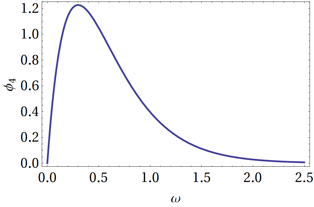
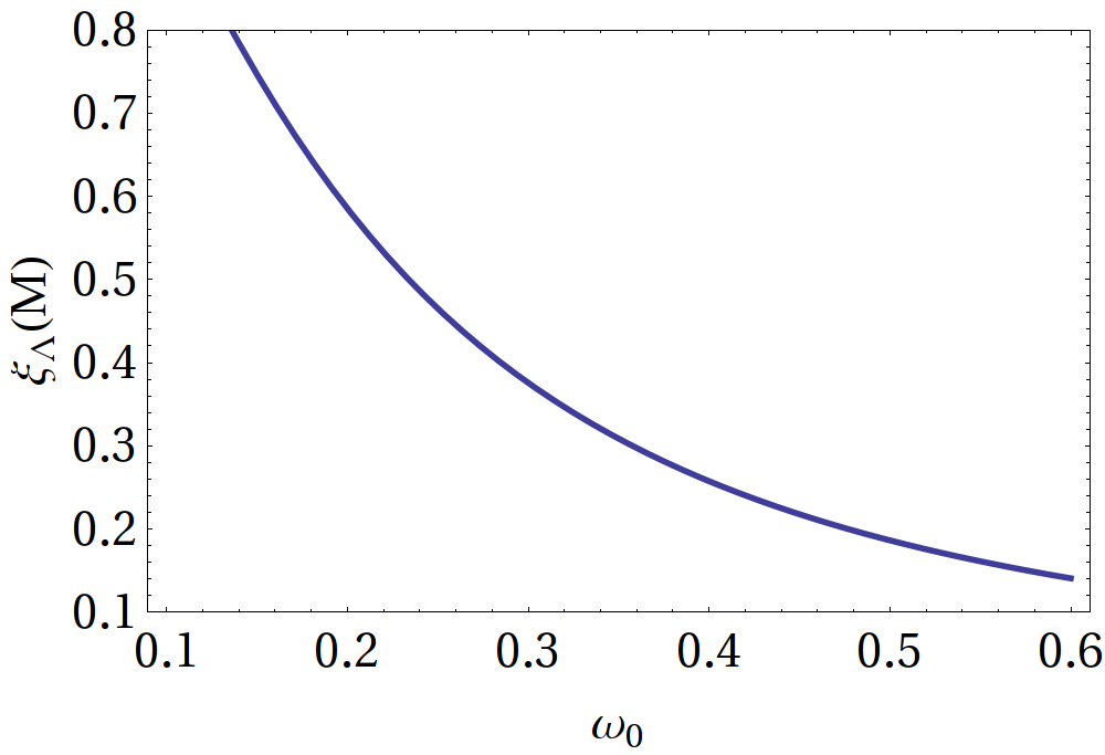
Figure 2: Left: Functional form of the partially integrated LCDA $\phi_{4}(\omega)$ for the exponential model and $\omega_{0}=300$ MeV. Right: Dependence of $\xi_{\Lambda}(n_{+}p^{\prime}=M_{\Lambda_{b}})$ on the value of $\omega_{0}$.

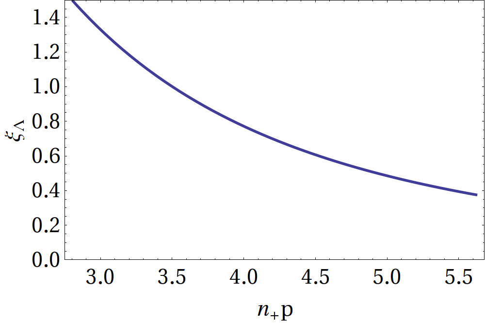
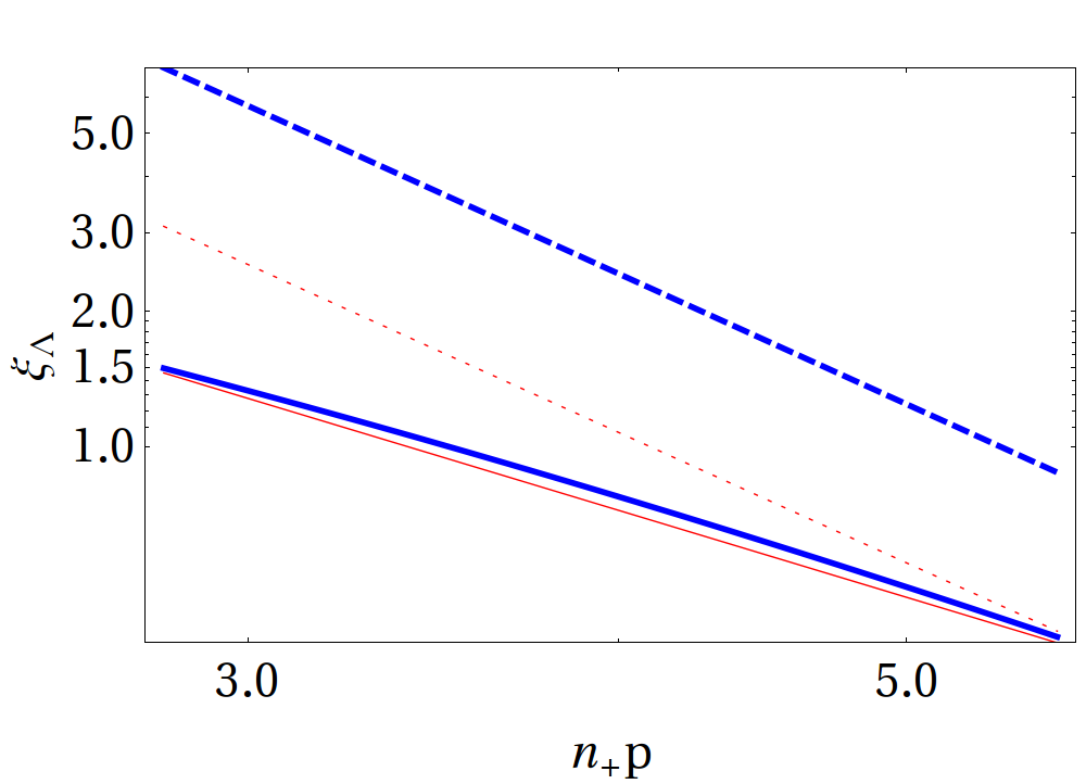
Figure 3: Dependence of the soft form factor on $(n_{+}p^{\prime})$. Left: energy dependence from the LO sum rule (3.39). Right: comparison of the LO sum rule (3.39) –thick solid line – , with the approximate formula (3.40) – thick dashed line –, and a power-like behaviour with $1/(n_{+}p^{\prime})^{3}$ (dash-dotted) or $1/(n_{+}p^{\prime})^{2}$ (dotted).

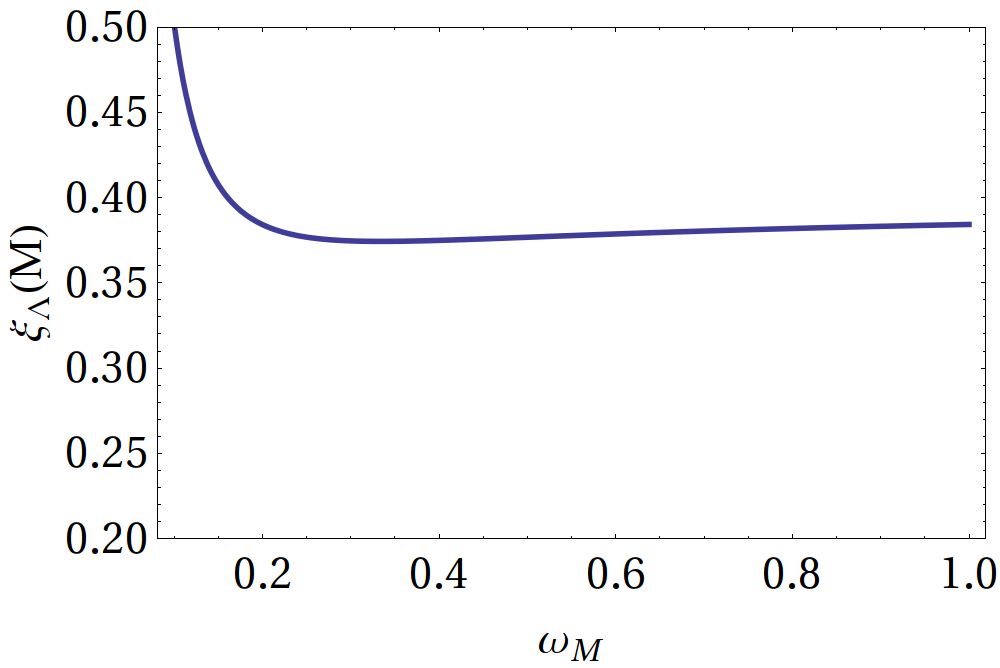
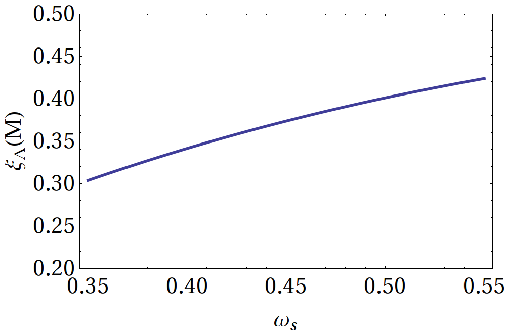
Figure 4: Dependence of the soft form factor on the sum-rule parameters (for maximal recoil, $n_{+}p^{\prime}=M_{\Lambda_{b}}$). Left: Dependence on the Borel parameter $\omega_{M}$. Right: Dependence on the threshold parameter $\omega_{s}$.

Taking these observations at face value, we have to conclude that the normalization of the $\Lambda_{b}\to\Lambda$ form factors at large recoil still suffers from sizeable uncertainties, mostly from the $\Lambda_{b}$ LCDAs and the threshold parameter. The same is true for the energy-dependence of the form factor which varies between a $1/(n_{+}p^{\prime})^{2}$ behaviour (small values of $\omega_{0}$) and a $1/(n_{+}p^{\prime})^{3}$ behaviour (large values of $\omega_{0}$). Independent information on the LCDA $\phi_{4}(\omega)$ and/or on the $\Lambda_{b}\to\Lambda$ form factors at intermediate momentum transfer from Lattice QCD would clearly be helpful in this context.

4.2 Form-Factor Ratios

The symmetry relations between the individual $\Lambda_{b}\to\Lambda$ form factors receive perturbative and non-perturbative corrections. Let us first consider the corrections from the exchange of one hard-collinear gluon, contributing to the function $\Delta\xi_{\Lambda}$ as estimated from the sum rule in (3.65). For the default values of the hadronic input parameters, we take the same values as before, see Table 1. As the default value for the strong coupling constant at a hard-collinear scale, we use $\alpha_{s}\simeq\alpha_{s}(\mu=2~{}{\rm GeV})\simeq 0.3$. For the relevant LCDAs, we will again use the exponential model discussed in section D.1. With this, we obtain as our default estimate

$$\Delta\xi_{\Lambda}(n_{+}p^{\prime}=M_{\Lambda_{b}})\simeq-0.003\,,\qquad\frac{\Delta\xi_{\Lambda}}{\xi_{\Lambda}}\simeq-0.8\%\,.$$

We also find that the ratio $\Delta\xi_{\Lambda}/\xi_{\Lambda}$ exhibits a mild linear dependence on the (large) recoil-energy and a pronounced linear dependence on the parameter $\omega_{0}$ in the exponential model for the $\Lambda_{b}$ LCDAs, see Fig. 5. This is in qualitative agreement with the considerations after Eq. (3.66).

The dependence of $\Delta\xi_{\Lambda}$ on the sum-rule parameters is plotted in Fig. 6. The sensitivity to the Borel parameter $\omega_{M}$, again, is rather weak, while the dependence on the threshold parameter $\omega_{s}$ is somewhat weaker than for the soft form factor $\xi_{\Lambda}$. Because of the different systematics in (3.39, 3.65) related to the modelling of the continuum and the pollution from other baryonic resonances, the dependence of the ratio $\Delta\xi_{\Lambda}/\xi_{\Lambda}$ on the sum rule parameters is difficult to estimate numerically. As already emphasized, the dependence on the light and heavy decay constants drops out in the ratio $\Delta\xi_{\Lambda}/\xi_{\Lambda}$. The overall dependence on the renormalization scale used for the strong coupling constant has to be resolved by calculating higher-order radiative corrections to $\Delta\xi_{\Lambda}$ in SCET.

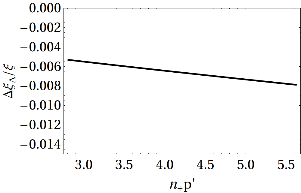
Figure 5: Form-factor correction $\Delta\xi_{\Lambda}/\xi_{\Lambda}$ from the exchange of one hard-collinear gluon from SCET sum rules. Left: Energy dependence from the LO sum rules (3.39, 3.65). Right: Dependence on the parameter $\omega_{0}$ characterizing the LCDAs of the $\Lambda_{b}$ baryon.

Figure 6: Dependence on $\Delta\xi_{\Lambda}$ on the sum-rule parameters (for $n_{+}p^{\prime}=M_{\Lambda_{b}}$). Left: Dependence on the Borel parameter $\omega_{M}$. Right: Dependence on the threshold parameter $\omega_{s}$.

The above result can be turned into an estimate for form-factor ratios appearing in physical decay observables. As an example, we discuss the ratios

$$\frac{h_{\perp}}{f_{\perp}}\,,\qquad\frac{\tilde{h}_{\perp}}{g_{\perp}}\,,$$

appearing in the forward-backward asymmetry for $\Lambda_{b}\to\Lambda\mu^{+}\mu^{-}$, see below. Including the effect of hard-vertex corrections to ${\cal O}(\alpha_{s})$ accuracy, we obtain the results shown in Fig. 7, where we have used

$$\alpha_{s}(m_{b})\simeq 0.2$$

in the hard vertex corrections. As one can see, the corrections to the form-factor ratios are dominated by the hard gluon effects in the matching coefficients for the decay currents.

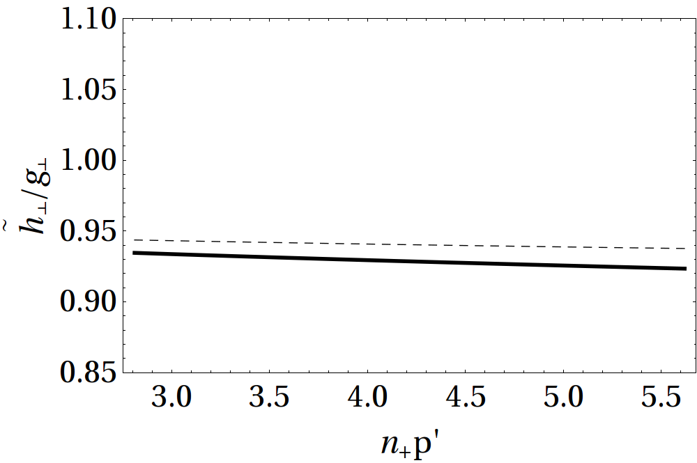
Figure 7: Form-factor ratios including ${\cal O}(\alpha_{s})$ corrections from hard (dashed line) and hard plus hard-collinear (solid line) gluon exchange, as a function of the recoil energy $(n_{+}p^{\prime})$: Left: The ratio $h_{\perp}/f_{\perp}$. Right: The ratio $\tilde{h}_{\perp}/g_{\perp}$.

4.3 $\Lambda_{b}\to\Lambda\mu^{+}\mu^{-}$ Observables

The general expressions for the double-differential $\Lambda_{b}\to\Lambda\mu^{+}\mu^{-}$ decay rate (excluding the non-factorisable contributions, see below) are summarized in Appendix A. Our default values for the form-factor estimates, in the large-recoil region, yield branching ratios which are slightly higher than the central experimental values reported by CDF [10] (and compatible with an independent theoretical estimate in [3]) within the theoretical and experimental uncertainties, see Fig. 8 (in view of the large hadronic uncertainties, the spectator effects from $\Delta\xi_{\Lambda}$ represent a sub-leading effect and are not included here for simplicity).

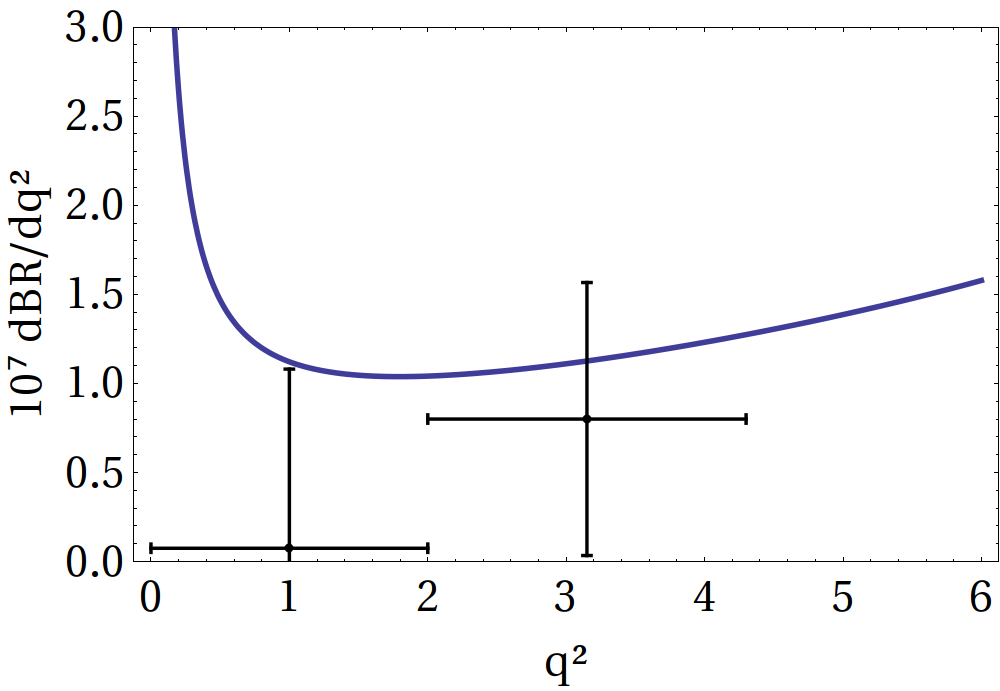
Figure 8: Differential branching ratio for $\Lambda_{b}\to\Lambda\mu^{+}\mu^{-}$ in units of $10^{-7}$ as a function of $q^{2}$ at large recoil. The theoretical estimate refers to the SCET limit, and the data points are taken from CDF [10]. The (substantial) theoretical uncertainties are not shown.

The functions describing the transverse and longitudinal rate, and the forward-backward asymmetry become particularly simple in the SCET limit, where all rates are proportional to the unique form factor $\xi_{\Lambda}(n_{+}p^{\prime})$, and $m_{\Lambda}\ll M_{\Lambda_{b}}$. To first approximation, the following ratios of observables are thus independent of hadronic form-factor uncertainties,

$$\frac{H_{L}(q^{2})}{H_{T}(q^{2})} \simeq\frac{q^{2}}{2M_{\Lambda_{b}}^{2}}\cdot\frac{\left|M_{\Lambda_{b}}^{2}\,C_{9}^{\rm eff}(q^{2})+2M_{b}M_{\Lambda_{b}}\,C_{7}^{\rm eff}\right|^{2}+\left|M_{\Lambda_{b}}^{2}\,C_{10}\right|^{2}}{\left|q^{2}\,C_{9}^{\rm eff}(q^{2})+2M_{b}M_{\Lambda_{b}}\,C_{7}^{\rm eff}\right|^{2}+\left|q^{2}\,C_{10}\right|^{2}}\,,$$ (4.67)

and

$$\frac{H_{A}(q^{2})}{H_{T}(q^{2})} \simeq-\frac{2\,{\rm Re}\left[\left(q^{2}\,C_{9}^{\rm eff}(q^{2})+2M_{b}M_{\Lambda_{b}}\,C_{7}^{\rm eff}\right)^{*}q^{2}\,C_{10}\right]}{\left|q^{2}\,C_{9}^{\rm eff}(q^{2})+2M_{b}M_{\Lambda_{b}}\,C_{7}^{\rm eff}\right|^{2}+\left|q^{2}\,C_{10}\right|^{2}}\,.$$ (4.68)

In particular, the leading-order result for the forward-backward asymmetry zero, $q_{0}^{2}$, is determined by the same relation between Wilson coefficients,

$${\rm Re}\left[q^{2}\,C_{9}^{\rm eff}(q^{2})+2M_{b}M_{\Lambda_{b}}\,C_{7}^{\rm eff}\right]_{q^{2}=q_{0}^{2}} \simeq 0\,,$$ (4.69)

as known from the inclusive $b\to s\ell^{+}\ell^{-}$ or exclusive $B\to K^{*}\ell^{+}\ell^{-}$ decays (see [29] and references therein).

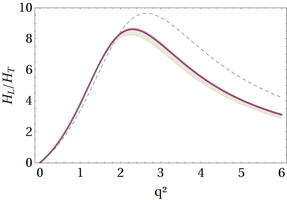
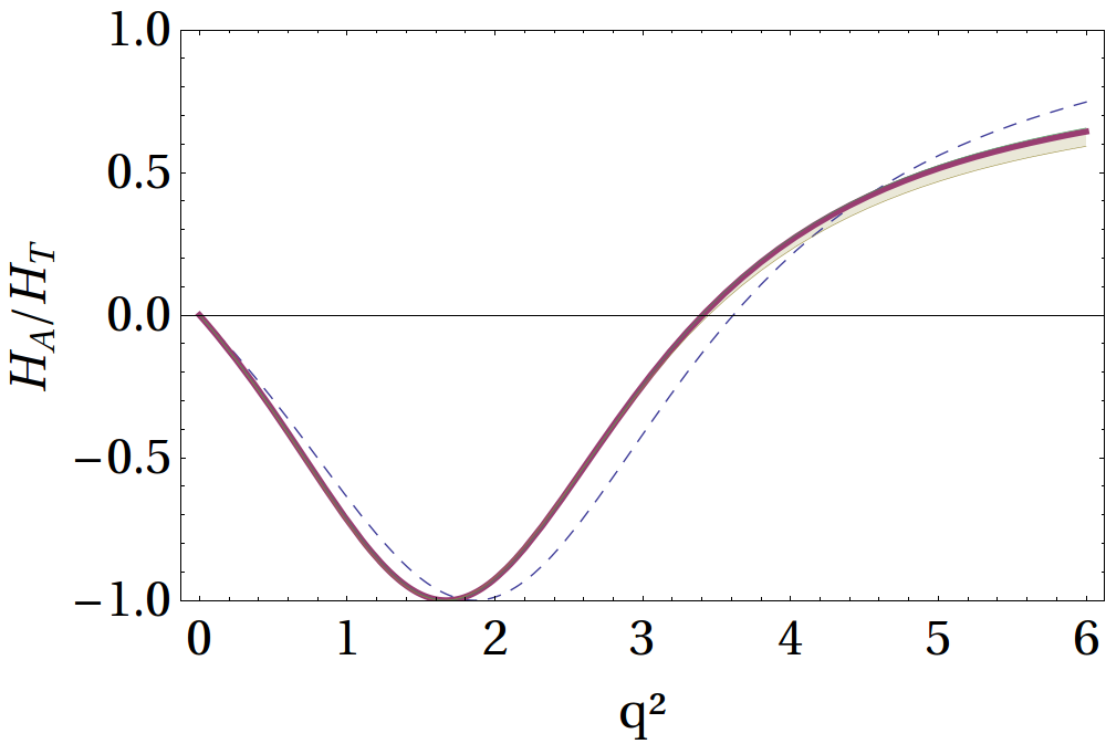
Figure 9: Ratios of observables, $H_{L}/H_{T}$ (left) and $H_{A}/H_{T}$ (right) as a function of $q^{2}$. The dashed line indicates the SCET limit (4.67, 4.68). The solid line includes the default estimates for the form-factor corrections from hard gluons, $C_{f_{i}}$, and hard-collinear gluons, $\Delta\xi_{\Lambda}$, as well as the kinematic corrections of order $m_{\Lambda}/M_{\Lambda_{b}}$. In order to illustrate the (tiny) uncertainty from the variation of $\Delta\xi_{\Lambda}/\xi_{\Lambda}$, we have inflated the error to an interval $[25\%,400\%]$ of its default value.

Our numerical estimates for the ratios $H_{L}/H_{T}$ and $H_{A}/H_{T}$ as a function of $q^{2}$ are plotted in Fig. 9, where we compare the SCET limit (4.67,4.68) with the more general result given in (A.82) in the Appendix (which, however, still misses the non-factorisable results). In the numerical analysis, the Wilson coefficients $C_{1-7}$ are included to leading-logarithmic accuracy, and the Wilson coefficients $C_{9,10}$ to next-to-leading logarithmic accuracy, with the numerical values taken from the analysis in [30]. As one can observe, the inclusion of the kinematic corrections of order $m_{\Lambda}/M_{\Lambda_{b}}$ together with the perturbative corrections to the form-factor relations leads to a significant effect in the ratio $H_{L}/H_{T}$ above $q^{2}=2$ GeV², whereas the ratio $H_{A}/H_{T}$ is not very much affected. In particular, we only find a small shift in the value of the forward-backward asymmetry zero,

$$q_{0}^{2} =\left\{\begin{array}[]{lr}3.6~{}{\rm GeV}^{2}&\qquad\mbox{\small(SCET limit),}\\ 3.4~{}{\rm GeV}^{2}&\qquad\mbox{\small(incl.\ corrections).}\end{array}\right.$$ (4.72)

Because of the small imaginary part of the term $(q^{2}C_{9}^{\rm eff}(q^{2})+2M_{b}M_{\Lambda_{b}}C_{7}^{\rm eff})$ in the large-recoil region, the function $H_{A}/H_{T}$ also develops a pronounced minimum with $H_{A}\simeq-H_{T}$. Again, its position is only slightly shifted from $q^{2}\simeq 1.9~{}{\rm GeV}^{2}$ in the SCET limit, to $q^{2}\simeq 1.7~{}{\rm GeV}^{2}$. Notice that the function $\Delta\xi_{\Lambda}$, which describes the spectator corrections to the form factors, enters the above observables with an additional suppression factor $2m_{\Lambda}/M_{\Lambda_{b}}\sim 40\%$, and therefore, even if – as indicated – we assign a large uncertainty to the ratio $\Delta\xi_{\Lambda}/\xi_{\Lambda}$, the considered ratios do not change a lot. The hard vertex corrections from the SCET matching coefficients $C_{f_{i}}$ and the purely kinematic corrections are thus responsible for the dominant numerical effect, together with the unspecified uncertainties from non-factorizable and power corrections.

5 Conclusions and Outlook

In this article, we have systematically investigated the form factors entering the baryonic $\Lambda_{b}\to\Lambda\ell^{+}\ell^{-}$ transitions in the framework of soft-collinear effective theory (SCET). As a starting point, we have introduced an improved form-factor parametrization, which leads to simple symmetry relations in the limit of heavy $b$-quark mass $m_{b}$ and/or large recoil-energy $E_{\Lambda}$ to the $\Lambda$ baryon, and which yields simple expressions for partial decay widths and decay asymmetries. We have shown that in the large recoil-energy limit, the 10 physical form factors for $\Lambda_{b}\to\Lambda$ transitions reduce to a single “soft” function $\xi_{\Lambda}(E_{\Lambda})$, which can be defined as a matrix element of a universal decay current in SCET. The latter has been estimated from a sum-rule analysis of an SCET correlation function, where the light $\Lambda$ baryon is interpolated by a suitable 3-quark current, and the heavy $\Lambda_{b}$ baryon is described by its light-cone distribution amplitudes (LCDAs). We have studied the energy dependence of the soft form factor, and performed a critical analysis of the uncertainties arising from the parameters used for the description of the hadronic continuum contribution to the sum rule, and for the model of the LCDAs. Compared to the recent measurement of the partially integrated $\Lambda_{b}\to\Lambda\mu^{+}\mu^{-}$ rate, we have found agreement within still large experimental and theoretical uncertainties.

For phenomenological analyses related to precision tests of the SM or searches for new physics, it is more convenient to study decay asymmetries, where – to first approximation – the dependence on hadronic form factors drops out in the large recoil-energy limit. In contrast to the analogous mesonic transitions, both, the ratio $H_{L}/H_{T}$ of the longitudinal and transverse decay rate, as well as the ratio $H_{A}/H_{T}$ defining the forward-backward asymmetry zero normalized to the transverse rate, are independent of the hadronic form factors in the SCET limit. A potentially important source of corrections arises from short-distance gluon exchange between the partonic $b\to s\ell^{+}\ell^{-}$ transition and the spectator quarks in the baryons. We have shown that the leading effect can be described by a hadronic matrix element of a particular sub-leading decay current in SCET. In contrast to the mesonic $b\to s\ell^{+}\ell^{-}$ transitions, the so-defined correction term $\Delta\xi_{\Lambda}$ cannot be calculated within the QCD-factorization approach, because one of the two spectator quarks may still populate the kinematic endpoint region where the resulting convolution integrals are ill-defined (in Appendix D.2, we briefly discuss how this could be avoided by switching to a toy model with elementary light di-quark states in the baryons). Still, the function $\Delta\xi_{\Lambda}$ can be obtained from a sum-rule analysis of another SCET correlation function, and the contributions to the individual transition form factors can be identified. Numerically, we find that the corrections $\Delta\xi_{\Lambda}/\xi_{\Lambda}$ only amount to a few percent or less. The corresponding corrections to the decay asymmetries have been estimated as well, including the effect of $\alpha_{s}$-corrections to the Wilson coefficients appearing in the matching of QCD decay currents onto the leading SCET current, and kinematic corrections of order $m_{\Lambda}/M_{\Lambda_{b}}$.

Another source of (partially perturbatively calculable) corrections to $\Lambda_{b}\to\Lambda\ell^{+}\ell^{-}$ decay observables is related to so-called “non-factorisable” effects which cannot be described in terms of $\Lambda_{b}\to\Lambda$ form factors. A systematic analysis of these contributions – following the analogous case of $B\to K^{*}\ell^{+}\ell^{-}$ decays in [30] – is left for future work. Finally, sub-leading terms in the SCET decay currents and SCET interaction terms between soft and collinear fields will lead to power corrections involving sub-leading components of the $\Lambda_{b}$ wave functions described by a number of new independent LCDAs. Since, at the moment, only little is known about the partonic structure of the $\Lambda_{b}$ at sub-leading order, the non-perturbative power corrections remain an irreducible source of hadronic uncertainties in rare exclusive $b$-quark decays.

Note Added

The symmetry relations between baryonic form factors in the large-recoil limit have also been discussed in a related recent paper in [31]. We thank Thomas Mannel and Yu-Ming Wang for sharing their results with us prior to publication. T.F. would also like to thank Yu-Ming Wang for helpful discussions on the choice of interpolating currents.

Appendix A Differential Decay Widths for $\Lambda_{b}\to\Lambda\mu^{+}\mu^{-}$

In this appendix we provide the general formulas for the differential decay widths for the radiative $\Lambda_{b}\to\Lambda\mu^{+}\mu^{-}$ transitions in terms of the 10 helicity form factors defined in Sec. 2. As usual, we consider the center-of-mass frame of the lepton-pair, and define the angle $\theta$ between the $\Lambda_{b}$ baryon and the positively charged lepton. For simplicity, we consider massless leptons, such that $q^{2}=2\,k_{\ell^{+}}\cdot k_{\ell^{-}}$. We then have

$$p_{\Lambda_{b}}\cdot k_{\ell^{\pm}} =\frac{M_{\Lambda_{b}}^{2}-m_{\Lambda}^{2}+q^{2}\mp\lambda\,\cos\theta}{4}\,,\qquad p_{\Lambda}\cdot k_{\ell^{\pm}}=\frac{M_{\Lambda_{b}}^{2}-m_{\Lambda}^{2}-q^{2}\mp\lambda\,\cos\theta}{4}\,.$$ (A.73)

Here,

$$\lambda\equiv\sqrt{s_{+}s_{-}} =\sqrt{((M_{\Lambda_{b}}+m_{\Lambda})^{2}-q^{2})\,(M_{\Lambda_{b}}-m_{\Lambda})^{2}-q^{2})}\,,$$ (A.74)

is the usual phase-space factor. If we define

$$\frac{d^{2}\Gamma(\Lambda_{b}\to\Lambda\ell^{+}\ell^{-})}{dq^{2}\,d\cos\theta} \equiv\frac{3}{8}\left\{(1+\cos^{2}\theta)\,H_{T}(q^{2})+2\cos\theta\,H_{A}(q^{2})+2(1-\cos^{2}\theta)\,H_{L}(q^{2})\right\}\,,$$ (A.75)

and neglect non-factorisable contributions, the different contributions to the differential decay rate can be written in terms of the form factors in the helicity basis,

$$H_{T}(q^{2}) =\frac{\lambda\,q^{2}\,n}{96\pi^{3}M_{\Lambda_{b}}^{3}}\Bigg{\{}s_{-}\left(\left|C_{9}^{\rm eff}(q^{2})\,f_{\perp}+\frac{2M_{b}\,(M_{\Lambda_{b}}+m_{\Lambda})\,C_{7}^{\rm eff}}{q^{2}}\,h_{\perp}\right|^{2}+\left|C_{10}\,f_{\perp}\right|^{2}\right)$$ (A.76)

$$\phantom{\frac{\lambda\,q^{2}\,n}{96\pi^{3}M_{\Lambda_{b}}^{3}}}\quad+s_{+}\left(\left|C_{9}^{\rm eff}(q^{2})\,g_{\perp}+\frac{2M_{b}\,(M_{\Lambda_{b}}-m_{\Lambda})\,C_{7}^{\rm eff}}{q^{2}}\,\tilde{h}_{\perp}\right|^{2}+\left|C_{10}\,g_{\perp}\right|^{2}\right)\Bigg{\}}\,,$$ (A.77)

$$H_{A}(q^{2}) =-\frac{\lambda^{2}\,q^{2}\,n}{48\pi^{3}M_{\Lambda_{b}}^{3}}\,{\rm Re}\left[\left(C_{9}^{\rm eff}(q^{2})\,f_{\perp}+\frac{2M_{b}\,(M_{\Lambda_{b}}+m_{\Lambda})\,C_{7}^{\rm eff}}{q^{2}}\,h_{\perp}\right)^{*}\left(C_{10}g_{\perp}\right)\right.$$ (A.78)

$$\phantom{\frac{\lambda^{2}\,n\,q^{2}}{48\pi^{3}M_{\Lambda_{b}}^{3}}\,{\rm Re}}\qquad\left.+\left(C_{9}^{\rm eff}(q^{2})\,g_{\perp}+\frac{2M_{b}\,(M_{\Lambda_{b}}-m_{\Lambda})\,C_{7}^{\rm eff}}{q^{2}}\,\tilde{h}_{\perp}\right)^{*}\left(C_{10}f_{\perp}\right)\right]\,,$$ (A.79)

$$H_{L}(q^{2}) =\frac{\lambda\,n}{192\pi^{3}M_{\Lambda_{b}}^{3}}\Bigg{\{}s_{-}\,(M_{\Lambda_{b}}+m_{\Lambda})^{2}\left(\left|C_{9}^{\rm eff}(q^{2})\,f_{+}+\frac{2M_{b}\,C_{7}^{\rm eff}}{M_{\Lambda_{b}}+m_{\Lambda}}\,h_{+}\right|^{2}+\left|C_{10}\,f_{+}\right|^{2}\right)$$ (A.80)

$$\phantom{\frac{\lambda\,n}{192\pi^{3}M_{\Lambda_{b}}^{3}}}\quad+s_{+}\,(M_{\Lambda_{b}}-m_{\Lambda})^{2}\left(\left|C_{9}^{\rm eff}(q^{2})\,g_{+}+\frac{2M_{b}\,C_{7}^{\rm eff}}{M_{\Lambda_{b}}-m_{\Lambda}}\,\tilde{h}_{+}\right|^{2}+\left|C_{10}\,g_{+}\right|^{2}\right)\Bigg{\}}\,.$$ (A.81)

(A.82)

where

$$n =\frac{\alpha^{2}\,G_{F}^{2}}{8\pi^{2}}\,|V_{ts}V_{tb}|^{2}\,.$$ (A.83)

The functions become particularly simple in the SCET limit, where

$$H_{T}(q^{2}) \simeq\frac{\lambda^{2}\,q^{2}\,n}{48\pi^{3}M_{\Lambda_{b}}^{3}}\,|\xi_{\Lambda}(n_{+}p^{\prime})|^{2}\Bigg{\{}\left|C_{9}^{\rm eff}(q^{2})+\frac{2M_{b}M_{\Lambda_{b}}\,C_{7}^{\rm eff}}{q^{2}}\right|^{2}+\left|C_{10}\right|^{2}\Bigg{\}}\,,$$ (A.84)

$$H_{A}(q^{2}) \simeq-\frac{\lambda^{2}\,q^{2}\,n}{24\pi^{3}M_{\Lambda_{b}}^{3}}\,|\xi_{\Lambda}(n_{+}p^{\prime})|^{2}\,{\rm Re}\left[\left(C_{9}^{\rm eff}(q^{2})+\frac{2M_{b}M_{\Lambda_{b}}\,C_{7}^{\rm eff}}{q^{2}}\right)^{*}C_{10}\right]\,,$$ (A.85)

$$H_{L}(q^{2}) \simeq\frac{\lambda^{2}\,n}{96\pi^{3}M_{\Lambda_{b}}}\,|\xi_{\Lambda}(n_{+}p^{\prime})|^{2}\Bigg{\{}\left|C_{9}^{\rm eff}(q^{2})+\frac{2M_{b}}{M_{\Lambda_{b}}}\,C_{7}^{\rm eff}\right|^{2}+\left|C_{10}\right|^{2}\Bigg{\}}\,.$$ (A.86)

Appendix B Alternative Form-Factor Parametrizations

B.1 Convention by Chen and Geng

The form factors in [1], which have been commonly used in the recent literature, are related to ours as follows. For the vector form factors, we obtain

$$f_{0} =f_{1}+\frac{q^{2}}{M_{\Lambda_{b}}-m_{\Lambda}}\,f_{3}\,,\qquad f_{+}=f_{1}-\frac{q^{2}}{M_{\Lambda_{b}}+m_{\Lambda}}\,f_{2}\,,\qquad f_{\perp}=f_{1}-(M_{\Lambda_{b}}+m_{\Lambda})\,f_{2}\,.$$ (B.87)

Similarly, for the axial-vector form factors, one gets

$$g_{0} =g_{1}-\frac{q^{2}}{M_{\Lambda_{b}}+m_{\Lambda}}\,g_{3}\,,\qquad g_{+}=g_{1}+\frac{q^{2}}{M_{\Lambda_{b}}-m_{\Lambda}}\,g_{2}\,,\qquad g_{\perp}=g_{1}+(M_{\Lambda_{b}}-m_{\Lambda})\,g_{2}\,.$$ (B.88)

The tensor and pseudo-tensor form factors are related by

$$h_{+}=f_{2}^{T}-\frac{M_{\Lambda_{b}}+m_{\Lambda}}{q^{2}}\,f_{1}^{T}\,,\qquad h_{\perp}=f_{2}^{T}-\frac{1}{M_{\Lambda_{b}}+m_{\Lambda}}\,f_{1}^{T}\,,$$ (B.89)

and

$$\tilde{h}_{+}=g_{2}^{T}+\frac{M_{\Lambda_{b}}-m_{\Lambda}}{q^{2}}\,g_{1}^{T}\,,\qquad\tilde{h}_{\perp}=g_{2}^{T}+\frac{1}{M_{\Lambda_{b}}-m_{\Lambda}}\,g_{1}^{T}\,.$$ (B.90)

B.2 Symmetry-Based Form-Factor Parametrization

An alternative parametrization considers the different projections of the decay current in the heavy-quark and/or large-energy limit, respectively. On the heavy-quark side, we consider the heavy-baryon velocity $v^{\mu}=p^{\mu}/M_{\Lambda_{b}}$ such that $\hbox to0.0pt{\hbox to5.20601pt{\hfil/\hfil}\hss}v\,u_{\Lambda_{b}}(p)=u_{\Lambda_{b}}(p)$. Also taking into account the projections on the light-quark side (using parity invariance of strong interactions), we end up with the general expression

$$\langle\Lambda(p^{\prime},s^{\prime})|\bar{q}\,\Gamma\,b|\Lambda_{b}(p,s)\rangle =\xi_{ij}^{(\pm)}(v,p^{\prime})\,\bar{u}_{\Lambda}(p^{\prime},s^{\prime})\left\{\Gamma_{i}\,\frac{\hbox to0.0pt{\hbox to6.00235pt{\hfil/\hfil}\hss}n_{\pm}\hbox to0.0pt{\hbox to6.00235pt{\hfil/\hfil}\hss}n_{\mp}}{4}\,\Gamma\,\Gamma_{j}\right\}u_{\Lambda_{b}}(p,s)$$ (B.91)

where the basis of Dirac matrices can be chosen as

$$\Gamma_{i} =\{1,\gamma_{5},\gamma_{\perp}^{\alpha}\}\,,\qquad\Gamma_{j}=\{1,\gamma_{5},\vec{\gamma}_{\mu},\vec{\gamma}_{\mu}\gamma_{5}\}\,,$$ (B.92)

and $\gamma_{\perp}^{\alpha}=\gamma^{\alpha}-\frac{\hbox to0.0pt{\hbox to4.20164pt{\hfil/\hfil}\hss}n_{+}}{2}n_{-}^{\alpha}-\frac{\hbox to0.0pt{\hbox to4.20164pt{\hfil/\hfil}\hss}n_{-}}{2}n_{+}^{\alpha}$, while $\vec{\gamma}_{\mu}=\gamma_{\mu}-\hbox to0.0pt{\hbox to5.20601pt{\hfil/\hfil}\hss}v\,v_{\mu}$ etc. Here and in the following, we consider a frame where $\hbox to0.0pt{\hbox to5.03125pt{\hfil/\hfil}\hss}p^{\prime}_{\perp}=0$ and $v^{\mu}=(n_{-}^{\mu}+n_{+}^{\mu})/2$. The non-vanishing form factors are

$$\xi_{11}^{(\pm)}(v,p^{\prime}) \equiv A^{(\pm)}(v\cdot p^{\prime})\sim{\cal O}(1)\,,\qquad\xi_{13}^{(\pm)}(v,p^{\prime})\equiv\frac{p^{\prime}{}^{\mu}}{v\cdot p^{\prime}}\,B^{(\pm)}(v\cdot p^{\prime})\sim{\cal O}(\epsilon)\,,$$ (B.93)

$$\xi_{22}^{(\pm)}(v,p^{\prime}) \equiv C^{(\pm)}(v\cdot p^{\prime})\sim{\cal O}(\epsilon)\,,\qquad\xi_{24}^{(\pm)}(v,p^{\prime})\equiv\frac{p^{\prime}{}^{\mu}}{v\cdot p^{\prime}}\,D^{(\pm)}(v\cdot p^{\prime})\sim{\cal O}(\epsilon)\,,$$ (B.94)

$$\xi_{33}^{(\pm)}(v,p^{\prime}) \equiv\delta_{\alpha}^{\mu}\,E^{(\pm)}(v\cdot p^{\prime})\sim{\cal O}(\epsilon)\,,$$ (B.95)

$$\xi_{34}^{(\pm)}(v,p^{\prime}) \equiv i\epsilon_{\alpha}{}^{\mu\rho\sigma}\,\frac{v_{\rho}\,p^{\prime}_{\sigma}}{v\cdot p^{\prime}}\,F^{(\pm)}(v\cdot p^{\prime})\sim{\cal O}(\epsilon)\,,\qquad$$ (B.96)

From the above 12 form factors, again, only 10 are independent, after the e.o.m. constraints have been taken into account. Here, the indicated suppression of the form factors with $\epsilon=\Lambda/M$ refers to the violation of the heavy-quark spin symmetry. In addition, in the large recoil limit the contributions from the form factors with an index “$-$” are additionally suppressed. Therefore, we may neglect the 5 form factors $B^{(-)}$ through $F^{(-)}$, which is a good approximation, because

• In the HQET limit, $v\cdot p^{\prime}\sim{\cal O}(m_{\Lambda})$, their contribution is suppressed at least by a factor $\Lambda/M$.

• In the SCET limit, $n_{+}p^{\prime}\sim{\cal O}(M_{\Lambda_{b}})$, their contribution is suppressed by at least a factor $(\Lambda/M)^{2}$ (for non-factorizable effects) or $\alpha_{s}$ (for factorizable effects, see below).

We thus end up with a rather efficient description which combines the symmetry constraints in both cases and allows one to systematically take into account sub-leading corrections in the large-recoil limit, which are partially calculable in the framework of QCD factorization or light-cone sum rules. In this approximation, the 10 physical helicity form factors are related by 5 equations (for vanishing light quark masses, $m_{s}\to 0$),

$$f_{0} =\frac{M_{\Lambda_{b}}+m_{\Lambda}}{M_{\Lambda_{b}}-m_{\Lambda}}\,\frac{n_{+}p^{\prime}-m_{\Lambda}}{n_{+}p^{\prime}+m_{\Lambda}}\,f_{+}+\frac{M_{\Lambda_{b}}-n_{+}p^{\prime}}{M_{\Lambda_{b}}-m_{\Lambda}}\left(g_{\perp}-\frac{n_{+}p^{\prime}-m_{\Lambda}}{n_{+}p^{\prime}+m_{\Lambda}}\,f_{\perp}\right)\,,$$ (B.97)

$$g_{0} =\frac{M_{\Lambda_{b}}-m_{\Lambda}}{M_{\Lambda_{b}}+m_{\Lambda}}\,\frac{n_{+}p^{\prime}+m_{\Lambda}}{n_{+}p^{\prime}-m_{\Lambda}}\,g_{+}+\frac{M_{\Lambda_{b}}-n_{+}p^{\prime}}{M_{\Lambda_{b}}+m_{\Lambda}}\left(f_{\perp}-\frac{n_{+}p^{\prime}+m_{\Lambda}}{n_{+}p^{\prime}-m_{\Lambda}}\,g_{\perp}\right)\,,$$ (B.98)

$$\tilde{h}_{\perp} =\frac{M_{\Lambda_{b}}+m_{\Lambda}}{M_{\Lambda_{b}}-m_{\Lambda}}\,\frac{n_{+}p^{\prime}-m_{\Lambda}}{n_{+}p^{\prime}+m_{\Lambda}}\,h_{\perp}+\frac{M_{\Lambda_{b}}-n_{+}p^{\prime}}{M_{\Lambda_{b}}-m_{\Lambda}}\left(g_{\perp}-\frac{n_{+}p^{\prime}-m_{\Lambda}}{n_{+}p^{\prime}+m_{\Lambda}}\,f_{\perp}\right)\,,$$ (B.99)

and

$$h_{+} =\frac{M_{\Lambda_{b}}+m_{\Lambda}}{M_{b}}\,f_{+}+\frac{n_{+}p^{\prime}-\Lambda}{M_{b}}\left(f_{\perp}-\frac{n_{+}p^{\prime}+m_{\Lambda}}{n_{+}p^{\prime}-m_{\Lambda}}\,g_{\perp}\right)\,,$$ (B.100)

$$\tilde{h}_{+} =\frac{M_{\Lambda_{b}}-m_{\Lambda}}{M_{b}}\,g_{+}+\frac{n_{+}p^{\prime}-\Lambda}{M_{b}}\left(g_{\perp}-\frac{n_{+}p^{\prime}-m_{\Lambda}}{n_{+}p^{\prime}+m_{\Lambda}}\,f_{\perp}\right)\,.$$ (B.101)

Appendix C Corrections to SCET Symmetry Relations

C.1 Hard Vertex Corrections

The hard vertex corrections to the individual QCD decay currents have been discussed before [16, 17]. From the general 1-loop result in Eq. (28) in [16] we can deduce the corrections to the individual form factors in the helicity basis, $f_{i}=C_{f_{i}}\,\xi_{\Lambda}+\ldots$. Defining the renormalization scheme through $C_{f_{+}}=C_{g_{+}}\equiv 1$, this leads to

$$C_{f_{0}}=C_{g_{0}}=1+\frac{\alpha_{s}C_{F}}{4\pi}\,2(1-L)\,,\qquad C_{f_{\perp}}=C_{g_{\perp}}=1+\frac{\alpha_{s}C_{F}}{4\pi}\,L\,,$$ (C.102)

and

$$C_{h_{+}}=C_{\tilde{h}_{+}}=1+\frac{\alpha_{s}C_{F}}{4\pi}\left(\ln\frac{M_{b}^{2}}{\mu^{2}}-2(1-L)\right)\,,\qquad C_{h_{\perp}}=C_{\tilde{h}_{\perp}}=1+\frac{\alpha_{s}C_{F}}{4\pi}\left(\ln\frac{M_{b}^{2}}{\mu^{2}}-2\right)\,,$$ (C.103)

with the abbreviation

$$L\equiv-\frac{M_{b}^{2}-q^{2}}{q^{2}}\,\ln\left(1-\frac{q^{2}}{M_{b}^{2}}\right)\,.$$

C.2 Hard-Collinear Gluon Exchange

We consider the tree-level matching (in light-cone gauge), following [16]

$$\bar{q}\,\Gamma\,Q_{v} \simeq\,\bar{\xi}\,\tilde{\Gamma}\,h_{v}-\frac{1}{n_{+}p^{\prime}}\,\bar{\xi}\,g\hbox to0.0pt{\hbox to7.50002pt{\hfil/\hfil}\hss}A_{\perp}\,\frac{\hbox to0.0pt{\hbox to6.00235pt{\hfil/\hfil}\hss}n_{+}}{2}\,\Gamma\,h_{v}-\frac{1}{M_{b}}\,\bar{\xi}\,\Gamma\,\frac{\hbox to0.0pt{\hbox to6.00235pt{\hfil/\hfil}\hss}n_{-}}{2}\,g\hbox to0.0pt{\hbox to7.50002pt{\hfil/\hfil}\hss}A_{\perp}\,h_{v}+\ldots$$ (C.104)

The hard-scattering contributions to the individual form factors in the large-recoil limit defined above can then be identified by means of (2.29) and setting $m_{\Lambda}\to 0$ and $M_{\Lambda_{b}}\to M_{b}\equiv M$. This is equivalent to using

$$A^{(-)} \simeq-\frac{2M}{m_{\Lambda}}\,\Delta\xi_{\Lambda}\,,\qquad E^{(+)}=F^{(+)}=\frac{1}{2}\,\Delta\xi_{\Lambda}$$ (C.105)

in (B.91). For the scalar and vector form factors, this yields

$$f_{0}(q^{2}) \simeq C_{f_{0}}\,\xi_{\Lambda}(n_{+}p^{\prime})-\frac{2M}{n_{+}p^{\prime}}\,\Delta\xi_{\Lambda}(n_{+}p^{\prime})\,,$$ (C.106)

$$f_{+}(q^{2}) \simeq C_{f_{+}}\,\xi_{\Lambda}(n_{+}p^{\prime})-2\left(2-\frac{M}{n_{+}p^{\prime}}\right)\,\Delta\xi_{\Lambda}(n_{+}p^{\prime})\,,$$ (C.107)

$$f_{\perp}(q^{2}) \simeq C_{f_{\perp}}\,\xi_{\Lambda}(n_{+}p^{\prime})+\frac{2M}{n_{+}p^{\prime}}\,\Delta\xi_{\Lambda}(n_{+}p^{\prime})\,,$$ (C.108)

where $C_{i}=C_{i}(\mu,n_{+}p^{\prime})$ denote the hard vertex coefficients as derived above. Similar relations can be obtained for the axial-vector and tensor form factors,

$$g_{0}(q^{2}) \simeq C_{g_{0}}\,\xi_{\Lambda}(n_{+}p^{\prime})+\frac{2M}{n_{+}p^{\prime}}\,\Delta\xi_{\Lambda}(n_{+}p^{\prime})\,,$$ (C.109)

$$g_{+}(q^{2}) \simeq C_{g_{+}}\,\xi_{\Lambda}(n_{+}p^{\prime})+2\left(2-\frac{M}{n_{+}p^{\prime}}\right)\,\Delta\xi_{\Lambda}(n_{+}p^{\prime})\,,$$ (C.110)

$$g_{\perp}(q^{2}) \simeq C_{g_{\perp}}\,\xi_{\Lambda}(n_{+}p^{\prime})-\frac{2M}{n_{+}p^{\prime}}\,\Delta\xi_{\Lambda}(n_{+}p^{\prime})\,,$$ (C.111)

and

$$h_{+}(q^{2}) \simeq C_{h_{+}}\,\xi_{\Lambda}(n_{+}p^{\prime})+\frac{2M}{n_{+}p^{\prime}}\,\Delta\xi_{\Lambda}(n_{+}p^{\prime})\,,$$ (C.112)

$$h_{\perp}(q^{2}) \simeq C_{h_{\perp}}\,\xi_{\Lambda}(n_{+}p^{\prime})-2\left(1-\frac{M}{n_{+}p^{\prime}}\right)\Delta\xi_{\Lambda}(n_{+}p^{\prime})\,,$$ (C.113)

and

$$\tilde{h}_{+}(q^{2}) \simeq C_{\tilde{h}_{+}}\,\xi_{\Lambda}(n_{+}p^{\prime})-\frac{2M}{n_{+}p^{\prime}}\,\Delta\xi_{\Lambda}(n_{+}p^{\prime})\,,$$ (C.114)

$$\tilde{h}_{\perp}(q^{2}) \simeq C_{\tilde{h}_{\perp}}\,\xi_{\Lambda}(n_{+}p^{\prime})+2\left(1-\frac{M}{n_{+}p^{\prime}}\right)\Delta\xi_{\Lambda}(n_{+}p^{\prime})\,.$$ (C.115)

C.3 Form-Factor Relations to ${\cal O}(\alpha_{s})$ Accuracy

To first order in the strong coupling constant, the hard vertex corrections and the spectator scattering corrections only provide 5 independent Dirac structures. As a consequence, after inclusion of ${\cal O}(\alpha_{s})$ corrections, from the 10 helicity form factors only 5 are still linearly independent. The 5 symmetry relations which are unaffected by ${\cal O}(\alpha_{s})$ radiative corrections can be summarized as

$$\frac{f_{0}+h_{+}}{g_{0}+\tilde{h}_{+}}=\frac{f_{\perp}-h_{+}}{g_{\perp}-\tilde{h}_{+}}=\frac{f_{+}+h_{+}-2h_{\perp}}{g_{+}+\tilde{h}_{+}-2\tilde{h}_{\perp}}$$ (C.116)

$$=-\frac{2(f_{+}-f_{\perp})+h_{+}-h_{\perp}}{2(g_{+}-g_{\perp})+\tilde{h}_{+}-\tilde{h}_{\perp}}=-\frac{M^{2}-2q^{2}}{M^{2}}\,\frac{h_{+}-\tilde{h}_{+}}{f_{+}-g_{+}}\ =\ 1\,.$$ (C.117)

Appendix D Light-Cone Distribution Amplitudes

Light-cone distribution amplitudes (LCDAs) are introduced as matrix elements of non-local QCD light-ray operators between the considered baryon states and the vacuum.

D.1 Distribution Amplitudes for the $\Lambda_{b}$ baryon

For the heavy $\Lambda_{b}$ baryon, we follow the definitions in [14] and consider the following two projections (two others are not shown),

$$\epsilon^{abc}\,\langle 0|\left(u^{a}(t_{1}n_{-})\,C\,\gamma_{5}\hbox to0.0pt{\hbox to6.00235pt{\hfil/\hfil}\hss}n_{-}\,d^{b}(t_{2}n_{-})\right)h^{c}_{v}(0)|\Lambda_{b}(v,s)\rangle =f^{(2)}_{\Lambda_{b}}\,\Psi_{2}(t_{1},t_{2})\,u_{\Lambda_{b}}(v,s)\,,$$

$$\epsilon^{abc}\,\langle 0|\left(u^{a}(t_{1}n_{-})\,C\,\gamma_{5}\hbox to0.0pt{\hbox to6.00235pt{\hfil/\hfil}\hss}n_{+}\,d^{b}(t_{2}n_{-})\right)h^{c}_{v}(0)|\Lambda_{b}(v,s)\rangle =f^{(2)}_{\Lambda_{b}}\,\Psi_{4}(t_{1},t_{2})\,u_{\Lambda_{b}}(v,s)\,.$$ (D.118)

The so-defined LCDAs in position space have a Fourier expansion,

$$\Psi_{i}(t_{1},t_{2}) =\int_{0}^{\infty}d\omega_{1}\int_{0}^{\infty}d\omega_{2}\,e^{-i(t_{1}\omega_{1}+t_{2}\omega_{2})}\,\psi_{i}(\omega_{1},\omega_{2})$$ (D.119)

$$=\int_{0}^{\infty}d\omega\,\omega\int_{0}^{1}du\,e^{-i\omega(t_{1}u+t_{2}\bar{u})}\,\tilde{\psi}_{i}(\omega,u)\,.$$ (D.120)

Here, the first alternative refers to a function of the two light-cone momenta $\omega_{1,2}=(n_{-}k_{1,2})$ of the two light quarks in the heavy baryon, while the second alternative considers the total light-cone momentum $\omega=\omega_{1}+\omega_{2}$ and the momentum fractions $u=\omega_{1}/\omega$, $\bar{u}=1-u=\omega_{2}/\omega$ (notice the additional factor of $\omega$ in the Fourier integral in the latter case). The normalization factors $f_{\Lambda_{b}}^{(1,2)}$ have mass-dimension 3 and are scale-dependent. For numerical estimates, we will use $f_{\Lambda_{b}}^{(i)}\simeq 0.030\pm 0.005~{}{\rm GeV}^{3}$. The LCDAs $\psi_{i}(\omega_{1},\omega_{2})$ in momentum space have mass-dimension $(-2)$ and are scale-dependent, too. More details can be found in [14].

The above definitions can be converted into momentum-space representations for the $\Lambda_{b}$ distribution amplitudes, following the analogous procedure that has been explained in detail for the $B$-meson LCDA in [16]. Taking an arbitrary light-like vector $y^{\mu}$ and defining $t=v\cdot y$, we can write the most general Lorentz decomposition in the heavy-quark limit,

$$\epsilon^{abc}\,\langle 0|\left(u^{a}(\tau_{1}y)\,C\gamma_{5}\gamma_{\mu}\,d^{b}(\tau_{2}y)\right)h^{c}_{v}(0)|\Lambda_{b}(v,s)\rangle$$ (D.121)

$$= f^{(2)}_{\Lambda_{b}}\left(v_{\mu}\,\Psi_{2}(\tau_{1},\tau_{2})+\frac{\Psi_{4}(\tau_{1},\tau_{2})-\Psi_{2}(\tau_{1},\tau_{2})}{2t}\,y_{\mu}\right)u_{\Lambda_{b}}(v,s)\,.$$ (D.122)

This can be turned into

$$\epsilon^{abc}\,\langle 0|\left(u_{\alpha}^{a}(\tau_{1}y)\,d^{b}_{\beta}(\tau_{2}y)\right)h^{c}_{v}(0)|\Lambda_{b}(v,s)\rangle$$ (D.123)

$$= \frac{f^{(2)}_{\Lambda_{b}}}{4}u_{\Lambda_{b}}(v,s)\,\left[\left(\hbox to0.0pt{\hbox to5.20601pt{\hfil/\hfil}\hss}v\,\Psi_{2}(\tau_{1},\tau_{2})+\frac{\Psi_{4}(\tau_{1},\tau_{2})-\Psi_{2}(\tau_{1},\tau_{2})}{2t}\,\hbox to0.0pt{\hbox to5.2616pt{\hfil/\hfil}\hss}y\right)\gamma_{5}C^{-1}\right]_{\beta\alpha}$$ (D.124)

$$\quad+\mbox{2 more terms.}$$ (D.125)

In the convolution with hard-scattering kernels that have a power expansion in the transverse momenta $k_{1\perp}$ and $k_{2\perp}$ of the two light quarks in the $\Lambda_{b}$ baryon, and which have a corresponding sub-sub-leading dependence on $(n_{+}k_{i})$, the most general momentum-space projector

$$\frac{f^{(2)}_{\Lambda_{b}}}{4}u_{\Lambda_{b}}(v,s)\,\tilde{M}(k_{1},k_{2})_{\beta\alpha}\Big{|}_{k_{i}=\omega_{i}n_{+}/2}$$ (D.126)

reads [33]

$$\tilde{M}(k_{1},k_{2})= \left(\frac{\hbox to0.0pt{\hbox to6.00235pt{\hfil/\hfil}\hss}n_{+}}{2}\,\psi_{2}(\omega_{1},\omega_{2})+\frac{\hbox to0.0pt{\hbox to6.00235pt{\hfil/\hfil}\hss}n_{-}}{2}\,\psi_{4}(\omega_{1},\omega_{2})\right.$$ (D.127)

$$\qquad\quad\left.-\frac{1}{2}\,\gamma_{\mu}^{\perp}\,\int_{0}^{\omega_{1}}d\eta_{1}\left(\psi_{42}^{(1)}(\eta_{1},\omega_{2})-\psi_{X}(\eta_{1},\omega_{2})\right)\frac{\hbox to0.0pt{\hbox to6.00235pt{\hfil/\hfil}\hss}n_{+}\hbox to0.0pt{\hbox to6.00235pt{\hfil/\hfil}\hss}n_{-}}{4}\,\frac{\partial}{\partial k_{1\mu}^{\perp}}\right.$$ (D.128)

$$\qquad\quad\left.-\frac{1}{2}\,\gamma_{\mu}^{\perp}\,\int_{0}^{\omega_{1}}d\eta_{1}\left(\psi_{42}^{(1)}(\eta_{1},\omega_{2})+\psi_{X}(\eta_{1},\omega_{2})\right)\frac{\hbox to0.0pt{\hbox to6.00235pt{\hfil/\hfil}\hss}n_{-}\hbox to0.0pt{\hbox to6.00235pt{\hfil/\hfil}\hss}n_{+}}{4}\,\frac{\partial}{\partial k_{1\mu}^{\perp}}\right.$$ (D.129)

$$\qquad\quad\left.-\frac{1}{2}\,\gamma_{\mu}^{\perp}\,\int_{0}^{\omega_{2}}d\eta_{2}\left(\psi_{42}^{(2)}(\omega_{1},\eta_{2})-\psi_{X}(\omega_{1},\eta_{2})\right)\frac{\hbox to0.0pt{\hbox to6.00235pt{\hfil/\hfil}\hss}n_{-}\hbox to0.0pt{\hbox to6.00235pt{\hfil/\hfil}\hss}n_{+}}{4}\,\frac{\partial}{\partial k_{2\mu}^{\perp}}\right.$$ (D.130)

$$\qquad\quad\left.-\frac{1}{2}\,\gamma_{\mu}^{\perp}\,\int_{0}^{\omega_{2}}d\eta_{2}\left(\psi_{42}^{(2)}(\omega_{1},\eta_{2})+\psi_{X}(\omega_{1},\eta_{2})\right)\frac{\hbox to0.0pt{\hbox to6.00235pt{\hfil/\hfil}\hss}n_{+}\hbox to0.0pt{\hbox to6.00235pt{\hfil/\hfil}\hss}n_{-}}{4}\,\frac{\partial}{\partial k_{2\mu}^{\perp}}\right)\gamma_{5}C^{-1}$$ (D.131)

$$\qquad+\mbox{2 more terms.}$$ (D.132)

Here, $\psi_{42}^{(2)}(\omega_{1},\omega_{2})=\psi_{42}^{(1)}(\omega_{2},\omega_{1})$ and $\psi_{X}(\omega_{1},\omega_{2})=\psi_{X}(\omega_{2},\omega_{1})$ and

$$\psi_{42}^{(1)}(\omega_{1},\omega_{2})+\psi_{42}^{(2)}(\omega_{1},\omega_{2}) =\psi_{4}(\omega_{1},\omega_{2})-\psi_{2}(\omega_{1},\omega_{2})\,.$$ (D.133)

From this we see that $\psi_{2,4}$ play the analogous role as $\phi_{\pm}^{B}$ for the $B$-meson. The asymmetric combination of $\psi_{42}^{(1)}$ and $\psi_{42}^{(2)}$, as well as $\psi_{X}$ do not contribute in the collinear limit (D.125). However, they do contribute to the correlator used for the sum-rule estimate of $\Delta\xi_{\Lambda}$. They also allow one to derive approximate Wandzura-Wilczek relations from the equations of motion,

$$\hbox to0.0pt{\hbox to5.52084pt{\hfil/\hfil}\hss}k_{2}\tilde{M}(k_{1},k_{2})\simeq\tilde{M}(k_{1},k_{2})\hbox to0.0pt{\hbox to5.52084pt{\hfil/\hfil}\hss}k_{1}\simeq 0\,,$$ (D.134)

in the limit of vanishing LCDAs with $n>3$ partons.

Parametrizations for the functional form of the LCDAs have been derived from a sum-rule analysis in [14]. In this paper, we will use a simple model which is based on an exponential ansatz suppressing large values of $(v\cdot k_{1,2})$, where $k_{1,2}$ are the on-shell momenta for the light quarks in the $\Lambda_{b}$,

$$f(v\cdot k_{1},v\cdot k_{2}) :=\frac{1}{\omega_{0}^{6}}\,e^{-(v\cdot k_{1}+v\cdot k_{2})/\omega_{0}}\,.$$ (D.135)

where $\omega_{0}\sim\Lambda_{\rm had}$ is a measure for the typical momentum of the di-quark. We then may use

$$\psi_{2}(\omega_{1},\omega_{2}) =\int_{0}^{\infty}dk_{1\perp}^{2}\,dk_{2\perp}^{2}\,f\left(\omega_{1}+\frac{k_{1\perp}^{2}}{\omega_{1}},\omega_{2}+\frac{k_{2\perp}^{2}}{\omega_{2}}\right)=\frac{\omega_{1}\,\omega_{2}\,e^{-(\omega_{1}+\omega_{2})/\omega_{0}}}{\omega_{0}^{4}}\,,$$ (D.136)

$$\psi_{4}(\omega_{1},\omega_{2}) =\int_{0}^{\infty}dk_{1\perp}^{2}\,dk_{2\perp}^{2}\,\frac{k_{1\perp}^{2}}{\omega_{1}^{2}}\,\frac{k_{2\perp}^{2}}{\omega_{2}^{2}}\,f\left(\omega_{1}+\frac{k_{1\perp}^{2}}{\omega_{1}},\omega_{2}+\frac{k_{2\perp}^{2}}{\omega_{2}}\right)=\frac{e^{-(\omega_{1}+\omega_{2})/\omega_{0}}}{\omega_{0}^{2}}\,,$$ (D.137)

where the pre-factors in the integrand of the second line correspond to the ratios $(n_{+}k_{i})/(n_{-}k_{i})$ taking into account that $\psi_{2}$ and $\psi_{4}$ change their role when switching $n_{+}\leftrightarrow n_{-}$. Also (see [33] for details),

$$\psi_{42}^{(1)}(\omega_{1},\omega_{2}) =\frac{\partial}{\partial\omega_{1}}\int_{0}^{\infty}dk_{1\perp}^{2}\,dk_{2\perp}^{2}\,\frac{k_{1\perp}^{2}}{2\omega_{1}}\left(1+\frac{k_{2\perp}^{2}}{\omega_{2}^{2}}\right)\,f\left(\omega_{1}+\frac{k_{1\perp}^{2}}{\omega_{1}},\omega_{2}+\frac{k_{2\perp}^{2}}{\omega_{2}}\right)$$ (D.138)

$$=\frac{(\omega_{0}-\omega_{1})(\omega_{0}+\omega_{2})}{2\omega_{0}^{4}}\,e^{-(\omega_{1}+\omega_{2})/\omega_{0}}\,,$$ (D.139)

$$\psi_{X}(\omega_{1},\omega_{2}) =-\frac{\partial}{\partial\omega_{1}}\int_{0}^{\infty}dk_{1\perp}^{2}\,dk_{2\perp}^{2}\,\frac{k_{1\perp}^{2}}{2\omega_{1}}\left(1-\frac{k_{2\perp}^{2}}{\omega_{2}^{2}}\right)\,f\left(\omega_{1}+\frac{k_{1\perp}^{2}}{\omega_{1}},\omega_{2}+\frac{k_{2\perp}^{2}}{\omega_{2}}\right)$$ (D.140)

$$=\frac{(\omega_{0}-\omega_{1})(\omega_{0}-\omega_{2})}{2\omega_{0}^{4}}\,e^{-(\omega_{1}+\omega_{2})/\omega_{0}}\,.$$ (D.141)

For later use, we also introduce the abbreviations

$$G(\omega_{1},\omega_{2}) =\int_{0}^{\omega_{1}}d\eta_{1}\left(\psi_{42}^{(1)}(\eta_{1},\omega_{2})-\psi_{X}(\eta_{1},\omega_{2})\right)\to\frac{\omega_{1}\omega_{2}}{\omega_{0}^{3}}\,e^{-(\omega_{1}+\omega_{2})/\omega_{0}}\,,$$ (D.142)

$$H(\omega_{1},\omega_{2}) =\int_{0}^{\omega_{2}}d\eta_{2}\left(\psi_{42}^{(2)}(\omega_{1},\eta_{2})+\psi_{X}(\omega_{1},\eta_{2})\right)\to\frac{\omega_{2}}{\omega_{0}^{2}}\,e^{-(\omega_{1}+\omega_{2})/\omega_{0}}\,.$$ (D.143)

The parameter $\omega_{0}$ has been estimated in [14] from a sum-rule analysis of $\tilde{\psi}_{2}(\omega,u)$ (also including corrections from higher-order Gegenbauer polynomials as a function of $(2u-1)$), and rather small values of order $200$ MeV or so have been found. In our numerical analysis in the main body of the text, we will use a somewhat higher value ($300$ MeV) as our default, but consider a rather large uncertainty associated to it.

D.2 Simplified Set-Up with Scalar Di-quark

For a simplified picture, one may also approximate the dynamics of the two light quarks in the $\Lambda_{b}$ baryon by an elementary scalar di-quark field $\varphi^{a}(x)$ in the $\bar{3}$ representation of $SU(3)_{C}$. In the HQET limit, the $\Lambda_{b}$ baryon could then be described by a single LCDA, defined as ($t=v\cdot z$)

$$\langle 0|\varphi^{a}(z)\,h^{a}_{v}(0)|\Lambda_{b}(v,s)\rangle =\hat{f}_{\Lambda_{b}}\,\Psi_{\Lambda_{b}}(t)\,u_{\Lambda_{b}}(v,s)\,,$$ (D.144)

and

$$\Psi_{\Lambda_{b}}(t) =\int_{0}^{\infty}d\omega\,e^{-it\omega}\,\phi_{\Lambda_{b}}(\omega)\,.$$ (D.145)

Here $\hat{f}_{\Lambda_{b}}$ has mass-dimension $+1$, and $\psi_{\Lambda_{b}}(\omega)$ has mass-dimension $-1$. The momentum-space projector in this case simply reads

$$\hat{f}_{\Lambda_{b}}\,\phi_{\Lambda_{b}}(\omega)\,u_{\Lambda_{b}}(v,s)\,.$$ (D.146)

Similarly, the $\Lambda$ baryon can be approximately described by two LCDAs, defined as

$$\langle\Lambda(p^{\prime},s^{\prime})|\bar{s}^{a}(z)\varphi^{a}{}^{\dagger}(0)|0\rangle =\int_{0}^{1}du\,e^{iu\,p^{\prime}\cdot z}\,\bar{u}_{\Lambda}(p^{\prime},s^{\prime})\left(\hat{f}_{\Lambda}^{(1)}\,\phi_{\Lambda}^{(1)}(u)-\sigma_{\mu\nu}p^{\prime}{}^{\mu}z^{\nu}\,\hat{f}_{\Lambda}^{(2)}\,\phi_{\Lambda}^{(2)}(u)\right)$$ (D.147)

which corresponds to a momentum-space projector

$$\bar{u}_{\Lambda}(p^{\prime},s^{\prime})\left(\hat{f}_{\Lambda}^{(1)}\,\phi_{\Lambda}^{(1)}(u)-\frac{i}{2}\,\sigma_{\mu\nu}\hat{f}_{\Lambda}^{(2)}\left\{n_{-}^{\mu}n_{+}^{\nu}\,\phi_{\Lambda}^{(2)}{}^{\prime}(u)-p^{\prime}{}^{\mu}\,\frac{\partial}{\partial k_{\perp}{}_{\nu}}\,\phi_{\Lambda}^{(2)}{}(u)\right\}\right)\,.$$ (D.148)

Soft form factor from simplified set-up:

We may use the di-quark approximation as a toy model, to obtain alternative expressions for the transition form factors from SCET sum rules. To this end, we consider a correlation function involving the interpolating current

$$\hat{J}_{\Lambda}(x) =\varphi^{a}(x)\,s^{a}(x)$$ (D.149)

with

$$\langle 0|\hat{J}_{\Lambda}(0)|\Lambda(p^{\prime},s^{\prime})\rangle =\hat{f}_{\Lambda}\,u_{\Lambda}(p^{\prime},s^{\prime})\,.$$ (D.150)

The remaining calculation is analogous to the realistic case considered in Sec 3.1, and yields the LO sum rule

$$e^{-m_{\Lambda}^{2}/(n_{+}p^{\prime})\hat{\omega}_{M}}\,\hat{f}_{\Lambda}\,\xi_{\Lambda}(n_{+}p^{\prime}) =\hat{f}_{\Lambda_{b}}\int_{0}^{\hat{\omega}_{s}}d\omega\,\phi_{\Lambda_{b}}(\omega)\,e^{-\omega/\hat{\omega}_{M}}\,,$$ (D.151)

with an according new threshold parameter $\hat{\omega}_{s}$ and Borel parameter $\hat{\omega}_{M}$.

Hard-collinear gluon correction from simplified set-up:

In the simplified toy model, as before, we define the correlation function using the interpolating current in (D.149),

$$\hat{\Pi}_{\Lambda}^{\mu}(n_{-}p^{\prime}) \equiv i\int d^{4}x\,e^{ip^{\prime}x}\langle 0|T\left[\frac{\hbox to0.0pt{\hbox to6.00235pt{\hfil/\hfil}\hss}n_{+}\hbox to0.0pt{\hbox to6.00235pt{\hfil/\hfil}\hss}n_{-}}{4}\,\hat{J}_{\Lambda}(x)\left[\bar{s}(0)\,\tilde{\Gamma}\,gA^{\mu}_{\perp}(0)\,b(0)\right]\right]|\Lambda_{b}(p)\rangle\,.$$ (D.152)

Evaluating the Feynman diagram (using scalar QCD for the di-quark in the $\bar{3}$ representation), we obtain

$$\hat{\Pi}_{\Lambda}^{\mu}(n_{-}p^{\prime}) =-ig_{s}^{2}C_{F}\,\hat{f}_{\Lambda_{b}}\,\int_{0}^{\infty}\!d\omega\,\phi_{\Lambda_{b}}(\omega)\int\!\frac{d^{D}l}{(2\pi)^{D}}\,\frac{1}{\left[l_{\perp}^{2}+(n_{+}l)(n_{-}l)\right]}\,\hbox to0.0pt{\hbox to5.00002pt{\hfil$l$\hfil}\hss}/_{\perp}l_{\perp}^{\mu}\,\tilde{\Gamma}\,u_{\Lambda_{b}}(v,s)$$ (D.153)

$$\qquad\times\,\frac{1}{\left[l_{\perp}^{2}+(n_{+}l)(n_{-}l-\omega)\right]}\,\frac{1}{\left[l_{\perp}^{2}+(n_{+}l+n_{+}p^{\prime})(n_{-}l+n_{-}p^{\prime}-\omega)\right]}\,.$$ (D.154)

The correlator can be calculated as before, leading to

$$\hat{\Pi}_{\Lambda}^{\mu}(n_{-}p^{\prime}) =-g_{s}^{2}C_{F}\,\hat{f}_{\Lambda_{b}}\,\gamma^{\mu}_{\perp}\,\tilde{\Gamma}\,u_{\Lambda_{b}}(v,s)\,\int_{0}^{\infty}\!d\omega\,\phi_{\Lambda_{b}}(\omega)\,\frac{1}{2}\,\int_{0}^{1}dz$$ (D.155)

$$\quad\times\int\!\frac{d^{D-2}l_{\perp}}{(2\pi)^{D-1}}\,\frac{(1-z)\,l_{\perp}^{2}/(D-2)}{[l_{\perp}^{2}-z(1-z)\,(n_{+}p^{\prime})(-n_{-}p^{\prime})]\,[l_{\perp}^{2}-z(1-z)\,(n_{+}p^{\prime})\,(\omega-n_{-}p^{\prime})]}\,,$$ (D.156)

In this case, the integral over transverse momenta is UV divergent and needs to be regularized, as indicated. However, the divergence only influences the real part, while the imaginary part gives a similar result as before, leading to

$$\hat{B}\hat{\Pi}_{\Lambda}^{\mu}(\hat{\omega}_{M})|_{\rm subtr.} =-\frac{1}{8}\,\frac{\alpha_{s}C_{F}}{2\pi}\,\hat{f}_{\Lambda_{b}}^{(2)}\,\gamma^{\mu}_{\perp}\,\tilde{\Gamma}\,u_{\Lambda_{b}}(v,s)\,\int_{0}^{\hat{\omega}_{s}}\!\frac{d\omega^{\prime}}{\hat{\omega}_{M}}\,e^{-\omega^{\prime}/\hat{\omega}_{M}}\int_{0}^{\infty}\!d\omega$$ (D.158)

$$\qquad\times\phi_{\Lambda_{b}}(\omega)\left(\theta(\omega^{\prime}-\omega)+\frac{\omega^{\prime}}{\omega}\,\theta(\omega-\omega^{\prime})\right)\,.$$ (D.159)

In the formal limit $\hat{\omega}_{s,M}\ll\omega_{0}$, this factorizes again, according to

$$\hat{B}\hat{\Pi}_{\Lambda}^{\mu}(\hat{\omega}_{M})|_{\rm subtr.} \simeq-\frac{1}{8}\,\frac{\alpha_{s}C_{F}}{2\pi}\,\hat{f}_{\Lambda_{b}}\,\gamma^{\mu}_{\perp}\,\tilde{\Gamma}\,u_{\Lambda_{b}}(v,s)\,\int_{0}^{\infty}\!\frac{d\omega}{\omega}\,\phi_{\Lambda_{b}}(\omega)\left(\hat{\omega}_{M}-e^{-\hat{\omega}_{s}/\hat{\omega}_{M}}(\hat{\omega}_{M}+\hat{\omega}_{s})\right)\,,$$ (D.160)

showing the same dependence on the sum-rule parameters as before in (3.66). For the hadronic side of the sum rule, in the simplified set-up, we now find

$$\hat{\Pi}_{\Lambda}^{\mu}\big{|}_{\rm reson.} =\frac{\hat{f}_{\Lambda}\,M_{\Lambda_{b}}\,\Delta\xi_{\Lambda}}{m_{\Lambda}^{2}-(n_{+}p^{\prime})(n_{-}p^{\prime})}\,\frac{\hbox to0.0pt{\hbox to6.00235pt{\hfil/\hfil}\hss}n_{+}\hbox to0.0pt{\hbox to6.00235pt{\hfil/\hfil}\hss}n_{-}}{4}\,(\hbox to0.0pt{\hbox to5.03125pt{\hfil/\hfil}\hss}p^{\prime}+m_{\Lambda})\,\gamma^{\mu}_{\perp}\,\tilde{\Gamma}\,u_{\Lambda_{b}}(v,s)$$ (D.161)

$$\simeq\frac{1}{n_{+}p^{\prime}}\,\frac{\hat{f}_{\Lambda}\,m_{\Lambda}\,M_{\Lambda_{b}}\,\Delta\xi_{\Lambda}}{m_{\Lambda}^{2}/(n_{+}p^{\prime})-(n_{-}p^{\prime})}\,\gamma^{\mu}_{\perp}\,\tilde{\Gamma}\,u_{\Lambda_{b}}(v,s)\,,$$ (D.162)

leading to the sum rule

$$e^{-m_{\Lambda}^{2}/(n_{+}p^{\prime})\hat{\omega}_{M}}\,\frac{\hat{f}_{\Lambda}\,M_{\Lambda_{b}}\,m_{\Lambda}}{\hat{\omega}_{M}\,n_{+}p^{\prime}}\,\Delta\xi_{\Lambda}$$ (D.163)

$$=-\frac{1}{8}\,\frac{\alpha_{s}C_{F}}{2\pi}\,\hat{f}_{\Lambda_{b}}\,\int_{0}^{\hat{\omega}_{s}}\!\frac{d\omega^{\prime}}{\hat{\omega}_{M}}\,e^{-\omega^{\prime}/\hat{\omega}_{M}}\int_{0}^{\infty}\!d\omega\,\phi_{\Lambda_{b}}(\omega)\left(\theta(\omega^{\prime}-\omega)+\frac{\omega^{\prime}}{\omega}\,\theta(\omega-\omega^{\prime})\right)\,.$$ (D.164)

In the simplified picture, the hard-collinear correction term $\Delta\xi_{\Lambda}$ could also be obtained from the QCD factorization approach, in complete analogy to the mesonic case discussed in [16]. This will lead to an (endpoint-converging) convolution of a hard-scattering kernel and the above LCDAs for light and heavy baryons in the di-quark approximation. In the heavy-mass limit, the above sum-rule expression can then be interpreted as a particular model for the light-cone wave function of the $\Lambda$ baryon, in a similar way as it has been discussed for the mesonic form factors in [19].

References

- [1] C. H. Chen and C. Q. Geng, “Baryonic rare decays of ,” Phys. Rev. D 64 (2001) 074001 [arXiv:hep-ph/0106193]; “Rare decays with polarized ,” Phys. Rev. D 63 (2001) 114024 [arXiv:hep-ph/0101171]; “Lepton asymmetries in heavy baryon decays of ,” Phys. Lett. B 516 (2001) 327 [arXiv:hep-ph/0101201]. C. H. Chen, C. Q. Geng and J. N. Ng, “T violation in decays with polarized ,” Phys. Rev. D 65 (2002) 091502 [arXiv:hep-ph/0202103].
- [2] Y. -L. Liu, L. -F. Gan, M. -Q. Huang, “The exclusive rare decay of heavy b-Baryons,” Phys. Rev. D83 (2011) 054007. [arXiv:1103.0081 [hep-ph]].
- [3] T. M. Aliev, K. Azizi, M. Savci, “Analysis of the decay in QCD,” Phys. Rev. D81 (2010) 056006. [arXiv:1001.0227 [hep-ph]]. T. M. Aliev and M. Savci, “Polarization effects in exclusive semileptonic decay,” JHEP 0605 (2006) 001 [arXiv:hep-ph/0507324]. T. M. Aliev, M. Savci and B. B. Sirvanli, “Double-lepton polarization asymmetries in decay in universal extra dimension model,” Eur. Phys. J. C 52 (2007) 375 [arXiv:hep-ph/0608143].
- [4] Y. -M. Wang, Y. -L. Shen, C. -D. Lu, “ transition form factors from QCD light-cone sum rules,” Phys. Rev. D80 (2009) 074012. [arXiv:0907.4008 [hep-ph]]. Y. m. Wang, Y. Li and C. D. Lu, “Rare Decays of and in the Light-cone Sum Rules,” Eur. Phys. J. C 59 (2009) 861 [arXiv:0804.0648 [hep-ph]].
- [5] G. Hiller and A. Kagan, “Probing for new physics in polarized decays at the Z,” Phys. Rev. D 65 (2002) 074038 [arXiv:hep-ph/0108074].
- [6] L. Oliver, J. C. Raynal and R. Sinha, “Note on new interesting baryon channels to measure the photon polarization in ,” Phys. Rev. D 82 (2010) 117502 [arXiv:1007.3632 [hep-ph]].
- [7] P. Colangelo, F. De Fazio, R. Ferrandes and T. N. Pham, “FCNC and transitions: Standard model versus a single universal extra dimension scenario,” Phys. Rev. D 77 (2008) 055019 [arXiv:0709.2817 [hep-ph]].
- [8] G. Hiller, M. Knecht, F. Legger and T. Schietinger, “Photon polarization from helicity suppression in radiative decays of polarized to spin-3/2 baryons,” Phys. Lett. B 649 (2007) 152 [arXiv:hep-ph/0702191].
- [9] L. Mott, W. Roberts, “Rare dileptonic decays of in a quark model,” [arXiv:1108.6129 [nucl-th]].
- [10] T. Aaltonen et al. [ CDF Collaboration ], “Observation of the Baryonic Flavor-Changing Neutral Current Decay ,” arXiv:1107.3753 [hep-ex].
- [11] T. Mannel, W. Roberts, Z. Ryzak, “Baryons in the heavy quark effective theory,” Nucl. Phys. B355 (1991) 38-53.
- [12] T. Mannel, S. Recksiegel, “Flavor changing neutral current decays of heavy baryons: The Case ,” J. Phys. G24 (1998) 979-990. [hep-ph/9701399].
- [13] J. Charles, A. Le Yaouanc, L. Oliver et al., “Heavy to light form-factors in the heavy mass to large energy limit of QCD,” Phys. Rev. D60 (1999) 014001. [hep-ph/9812358].
- [14] P. Ball, V. M. Braun, E. Gardi, “Distribution Amplitudes of the Baryon in QCD,” Phys. Lett. B665 (2008) 197-204. [arXiv:0804.2424 [hep-ph]].
- [15] Y. -L. Liu, M. -Q. Huang, “Distribution amplitudes of and and their electromagnetic form factors,” Nucl. Phys. A821 (2009) 80-105. [arXiv:0811.1812 [hep-ph]].
- [16] M. Beneke, Th. Feldmann, “Symmetry breaking corrections to heavy-to-light -meson form factors at large recoil,” Nucl. Phys. B592, 3-34 (2001). [hep-ph/0008255].
- [17] C. W. Bauer, S. Fleming, D. Pirjol, I. W. Stewart, “An Effective field theory for collinear and soft gluons: Heavy to light decays,” Phys. Rev. D63 (2001) 114020. [hep-ph/0011336].
- [18] M. Beneke, A. P. Chapovsky, M. Diehl, Th. Feldmann, “Soft collinear effective theory and heavy to light currents beyond leading power,” Nucl. Phys. B643 (2002) 431-476. [hep-ph/0206152]; M. Beneke, Th. Feldmann, “Factorization of heavy-to-light form factors in soft collinear effective theory,” Nucl. Phys. B685 (2004) 249-296. [hep-ph/0311335].
- [19] F. De Fazio, Th. Feldmann, T. Hurth, “Light-cone sum rules in soft-collinear effective theory,” Nucl. Phys. B733 (2006) 1-30. [hep-ph/0504088]; “SCET sum rules for and transition form factors,” JHEP 0802 (2008) 031. [arXiv:0711.3999 [hep-ph]].
- [20] A. Khodjamirian, T. Mannel, N. Offen, “Form-factors from light-cone sum rules with B-meson distribution amplitudes,” Phys. Rev. D75 (2007) 054013. [hep-ph/0611193]; S. Faller, A. Khodjamirian, C. .Klein, T. .Mannel, “ Form Factors from QCD Light-Cone Sum Rules,” Eur. Phys. J. C60 (2009) 603-615. [arXiv:0809.0222 [hep-ph]].
- [21] N. Kivel, M. Vanderhaeghen, “Soft spectator scattering in the nucleon form factors at large within the SCET approach,” Phys. Rev. D83 (2011) 093005. [arXiv:1010.5314 [hep-ph]].
- [22] C. G. Boyd, M. J. Savage, “Analyticity, shapes of semileptonic form-factors, and ,” Phys. Rev. D56 (1997) 303-311. [hep-ph/9702300].
- [23] A. Bharucha, Th. Feldmann, M. Wick, “Theoretical and Phenomenological Constraints on Form Factors for Radiative and Semi-Leptonic B-Meson Decays,” JHEP 1009 (2010) 090. [arXiv:1004.3249 [hep-ph]].
- [24] V. Braun, R. J. Fries, N. Mahnke et al., “Higher twist distribution amplitudes of the nucleon in QCD,” Nucl. Phys. B589 (2000) 381-409. [hep-ph/0007279].
- [25] B. O. Lange, M. Neubert, “Renormalization group evolution of the B-meson light-cone distribution amplitude,” Phys. Rev. Lett. 91 (2003) 102001. [hep-ph/0303082].
- [26] G. Bell, Th. Feldmann, “Modelling light-cone distribution amplitudes from non-relativistic bound states,” JHEP 0804 (2008) 061. [arXiv:0802.2221 [hep-ph]].
- [27] S. Descotes-Genon, N. Offen, “Three-particle contributions to the renormalisation of B-meson light-cone distribution amplitudes,” JHEP 0905 (2009) 091. [arXiv:0903.0790 [hep-ph]]; M. Knoedlseder, N. Offen, “Renormalisation of heavy-light light-ray operators,” [arXiv:1105.4569 [hep-ph]].
- [28] A. Khodjamirian, C. Klein, T. Mannel and Y. M. Wang, “Form Factors and Strong Couplings of Heavy Baryons from QCD Light-Cone Sum Rules,” arXiv:1108.2971 [hep-ph].
- [29] M. Antonelli et al., “Flavor Physics in the Quark Sector,” Phys. Rept. 494 (2010) 197-414. [arXiv:0907.5386 [hep-ph]].
- [30] M. Beneke, Th. Feldmann, D. Seidel, “Exclusive radiative and electroweak and penguin decays at NLO,” Eur. Phys. J. C41 (2005) 173-188. [hep-ph/0412400]; “Systematic approach to exclusive decays,” Nucl. Phys. B612 (2001) 25-58. [hep-ph/0106067].
- [31] T. Mannel and Y. M. Wang, “Heavy-to-light baryonic form factors at large recoil,” arXiv:1111.1849 [hep-ph].
- [32] G. Burdman, G. Hiller, “Semileptonic form-factors from decays in the large-energy limit,” Phys. Rev. D63 (2001) 113008. [hep-ph/0011266].
- [33] T. Feldmann, Y.-M. Wang, M.W.Y. Yip (2012 – in preparation).