Optimizing future dark energy surveys for model selection goals

Abstract

We demonstrate a methodology for optimizing the ability of future dark energy surveys to answer model selection questions, such as ‘Is acceleration due to a cosmological constant or a dynamical dark energy model?’. Model selection Figures of Merit are defined, exploiting the Bayes factor, and surveys optimized over their design parameter space via a Monte Carlo method. As a specific example we apply our methods to generic multi-fibre baryon acoustic oscillation spectroscopic surveys, comparable to that proposed for SuMIRe PFS, and present implementations based on the Savage–Dickey Density Ratio that are both accurate and practical for use in optimization. It is shown that whilst the optimal surveys using model selection agree with those found using the Dark Energy Task Force (DETF) Figure of Merit, they provide better informed flexibility of survey configuration and an absolute scale for performance; for example, we find survey configurations with close to optimal model selection performance despite their corresponding DETF Figure of Merit being at only 50% of its maximum. This Bayes factor approach allows us to interpret the survey configurations that will be good enough for the task at hand, vital especially when wanting to add extra science goals and in dealing with time restrictions or multiple probes within the same project.

1 Introduction

Cosmology has developed dramatically in recent years; from being restricted to the realms of philosophy, our observational abilities have advanced it to the point where we may obtain precise evidence with which to shape our models and understanding. In this age of precision cosmology, the fine tuning of surveys can dramatically improve their performance. This requires us to think in terms of designer surveys rather than using a build-and-point approach.

For any given problem in cosmology (we use that of dark energy hereafter) many surveys of varying capabilities will be proposed, and a combination will make it through the conceptual stages to see the light of night. For example, there are several stages defined by the Dark Energy Task Force (DETF) to classify dark energy surveys; stage II surveys are complete, e.g. the Sloan Digital Sky Survey (SDSS); several stage III surveys are now taking data, e.g. The Baryon Oscillation Spectroscopic Survey (BOSS) and WiggleZ, with others at the manufacturing stage, e.g. The Dark Energy Survey (DES) and the Hobby–Eberly Telescope Dark Energy EXperiment (HETDEX); and Stage IV surveys are still in the design phase e.g. BigBOSS, the Square Kilometre Array (SKA), the Wide-Field Infrared Survey Telescope (WFIRST), and the recently-approved Euclid satellite mission.

When considering the large investments of time, money and expertise involved in these projects, it is imperative that designers identify the survey configuration that maximises the science return. Given the number of surveys all targeting the same goal, it is also important that they identify the appropriate niche; doing so maximises the overall science return from the combined effort of all relevant surveys. Moreover, naive optimization can be wasteful unless there is an absolute scale of performance that can be used to determine survey configurations that are good enough for a given task, especially when dealing with time or cost restrictions, or with multiple probes within a survey. The importance of optimization for dark energy surveys was first stressed by Bassett (2005) and Bassett, Parkinson & Nichol (2005b).

The concept of optimization is universal to design, regardless of the product in hand; a scalar rating or Figure of Merit (FoM) is defined, and the configuration of product variables that optimizes this number is identified. When it comes to designing a survey’s observational parameters it is usual to exploit Monte Carlo Markov Chain (MCMC) methods to vary things like survey time, area, exposure time, and redshift range to identify the extreme of a FoM.

In developing their roadmap for the future, the Dark Energy Task Force defined a FoM for comparing proposed dark energy surveys. The FoM is based on parameter estimation, quantifying the errors measured on the $\Lambda\rm CDM$ values of the dark energy equation of state. This has subsequently become the standard for the quantification of dark energy survey performance. However the question we wish to answer in building these surveys asks: which of the models we have should be preferred; and if a single model cannot be selected outright, as is presently the case with the dark energy problem, which can we discount? The DETF approach skips this question and assumes that we already know the right model, the idea being that if the true parameter values lie outside of the 2-$\sigma$ error contours then the survey will be well placed to identify it. Whilst this does not seem an unreasonable presumption it has not been properly tested.

Bassett (2005) introduced the Integrated Parameter Space Optimization (IPSO) design framework to address this, proposing that the FoM be some function of the 1-$\sigma$ marginalized dark energy covariance matrix. In this paper we take a similar approach, but instead adopt FoMs that rate a survey’s ability to perform model selection, thereby directly optimizing for the survey’s designed objective.

It is highly problematic to use frequentist statistics to deal with model selection, whereas Bayesian statistics provides the perfect platform. In particular we employ the Bayes factor, which measures the increase of belief in one model over another that new data provides. A downside of parameter estimation ratings is that their scale is relative, providing no simple interpretation of when a survey is good enough for the job in hand. This is unfortunate as it is vital that money and effort does not get frittered away in making surveys arbitrarily more powerful, whilst promising no significant advances in our knowledge. The Bayes factor addresses this issue by providing an absolute scale; this is a big motivation for considering its use within forecasting and optimization [Mukherjee et al. 2006a, Trotta 2007a, Trotta 2007b].

In this paper we define our model selection FoMs in section 2; in section 3 we use a particular ground based dark energy survey aiming to exploit baryonic acoustic oscillations to identify practical implementations for each, and also to test their performance; and in section 4 we exploit these model selection ratings to optimize the baryon acoustic oscillation survey SuMIRe PFS (Subaru Measurement of Images and Redshifts Prime Focus Spectrograph) [Takada 2010, Takada & Silverman 2010].

It is worth noting that the implementations we investigate are relatively crude and there exists much room for refinements. However, our main motivation is to compare the performance of the model selection FoM to that of parameter estimation FoM; refinements to improve on computational efficiency have no influence on the outcome and are therefore superfluous at this point. Furthermore, as all optimizations to date exploit parameter estimation FoMs, we deem it sensible to identify ways in which these optimizations can be easily adapted to address their short-fallings.

2 Model selection optimization

2.1 Optimization details

Our principal goal is to introduce the concept of model selection optimization to astrophysics, the concept being a very general one. However, for concreteness we will focus throughout on a realistic scenario where the idea could be deployed, by considering optimization of baryon acoustic oscillation (BAO) surveys for dark energy that could be carried out by large multi-object spectrographs on eight-metre class telescopes.

This study builds on an optimization study that was carried out by Parkinson et al. (2010, henceforth P10). In brief, the survey modelled by this optimization comprised a 3000-fibre spectrograph mounted on a ground-based 8m optical-infrared telescope. The specifications used to model this survey are outlined in Table 1, and a full description can be found in Bassett, Nichol & Eisenstein (2005a). Ultimately this project (WFMOS) did not move forward to construction, but the concept and design lives on in the form of SuMIRe PFS, with the spectrograph to be mounted on the Subaru telescope. Other proposed spectroscopic BAO surveys include BigBOSS (Schlegel et al. 2011) and DESpec.

Constraint Parameter	Value
Total observing time	1500 hours
Field of view	$1.5^{o}$ diameter
$n_{\rm fibres}$	3000
Aperture	8m
Fibre diameter	1 arcsec
Overhead time between exposures	10 mins
Minimum exposure time	15 mins
Maximum exposure time	10 hours
Wavelength response	375 to 1000 nm
Width of redshift slices, $dz$	0.05

Table 1: Survey constraints used in modelling the multi-object spectrograph.

We model the survey to observe line emission of pre-selected active star-forming galaxies. Its wavelength coverage allows observation of the OII lines and the $4000\rm\AA$ break in the redshift range $0.1\leq z\leq 1.6$; this overall range is divided into sub-bins as per Figure 1 and the density throughout is fixed by that of the deepest redshift bin.

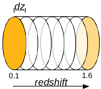
Figure 1: Representation of the $z$ binning method of the optimization code used.

Our optimization method closely follows that of P10, utilising Monte Carlo Markov Chain (MCMC) [Metropolis et al. 1953, Hastings 1970] methods to identify the survey configuration that maximises a FoM. The larger this rating the better the survey’s performance. The variables that describe each survey configuration are described in Table 2. Given that we already have dark energy constraints from the Sloan Digital Sky Survey (SDSS) and will soon have data from Planck, SDSS data and forecasts for the Planck data are included as prior information; again refer to P10 for details.

Survey Parameter	Symbol
Time allocated	$\tau$
Area covered	$A$
Minimum of redshift bin	$z_{\rm min}$
Maximum of redshift bin	$z_{\rm max}$
Number of pointings	$n_{\rm p}$

Table 2: Survey parameters varied by the optimization code, affecting the various FoM under consideration.

We wish to compare a parameter estimation FoM, that rates a survey’s ability to measure the parameters of interest assuming the true model is known, to model selection FoMs that recognise our uncertainty surrounding the most preferable model. The Dark Energy Task Force (DETF) FoM has been widely adopted by the cosmological community as the standard for comparison of dark energy surveys and their optimization [Albrecht et al. 2006]. As such, we take the DETF FoM as the parameter estimation baseline for comparison.

The DETF FoM makes use of the CPL [Chevallier & Polarski 2001, Linder 2003] parametrisation of the dark energy equation of state $w$, given by

$$w(a)=w_{0}+w_{a}\left(\frac{z}{1+z}\right)\,,$$ (1)

where $w_{0}$ is a constant characterising the behaviour of $w$ in the local universe and the constant $w_{a}$ characterises its redshift dependence. The DETF FoM is the inverse of the area confined within the 95% confidence level on $w_{0}$ and $w_{a}$ measurements, assuming throughout that $w_{0}=-1$ and $w_{a}=0$, i.e. $\Lambda\rm CDM$, is the true cosmological model. The smaller this area, the larger the FoM, and the more accurate the survey.

For each survey configuration, the optimization of P10 forecasts the errors on the measurable quantities $d_{A}$ and $H$ by using a 1D Fisher matrix based transfer function as derived by Seo & Eisenstein (2007). This returns the BAO distance errors as a function of survey properties and non-linearity. These errors are then translated onto $w_{0}$ and $w_{a}$, given by the inverse of the marginalised Fisher matrix i.e. $F^{-1}_{w_{0}w_{a}}$; from this the DETF FoM may be calculated:

$$\mathrm{FoM_{DETF}}=\frac{1}{\sqrt{\sigma^{2}_{w_{0}w_{0}}\sigma^{2}_{w_{a}w_{a}}-\sigma^{4}_{w_{0}w_{a}}}}=\frac{1}{\sqrt{\det F^{-1}_{w_{0}w_{a}}}}\,.$$

For detailed information on this optimization and Fisher matrix approach please refer to P10 and Parkinson et al. (2009).

2.2 Model selection FoM

As mentioned we use Bayesian Statistics as the foundation for our model selection FoMs. As this subject has been covered extensively in the literature, we will only provide an overview here. The basic laws of probability such as the multiplication rule were shown by Cox (1946) to be the mathematical framework of Boolean logic. Bayes theorem derives from direct application of this rule and provides a means to calculate the probability of a given model ($M$) (as per equation 2) or hypothesis ($\bm{\theta}$) in light of data ($D$) [Jeffreys 1961, Jaynes 2003, MacKay 2003, Gregory 2005]:

$$p(M\mid D)=\frac{p(D\mid M)\,p(M)}{p(D)}\,.$$ (2)

Bayesian statistics provide a natural framework for dealing with model selection and as such form the basis for the model selection FoM used in this paper.

From here on we use standard notation when referring to probabilities, e.g. $p(A\mid B,C)$ means the probability of $A$ given that $B$ and $C$ are true. In equation 2, $p(M\mid D)$ is referred to as the model posterior; $p(D\mid M)$ is the model likelihood, generally referred to as the evidence; the prior $p(M)$ characterises our state of knowledge before the data was collected; and the normalisation term is $p(D)$, the probability of the data.

The star of the show is the Bayes factor $B$ [Jeffreys 1961, Kass & Raftery 1995], which measures the increase of belief in one model over another given new data. Alternatively it can be considered as the change in model odds from before the data was considered to after. This scalar quantity is evaluated by taking the ratio of the evidence $E$ of one model given data, i.e. $p(D\mid M_{0})$, to that of another, $p(D\mid M_{1})$, as given in equation 3:

$$B=\frac{E(M_{0})}{E(M_{1})}=\frac{p(D\mid M_{0})}{p(D\mid M_{1})}\,.$$ (3)

The combination of model selection FoMs we use for this work takes account of the uncertainty in our knowledge. We allow the assumed model to vary through its values of $w_{0}$ and $w_{a}$, rather than fixing it to one fiducial model as is the case for the DETF FoM. The allowed models are restricted to a chosen region of $w_{0}$–$w_{a}$ parameter space, in which $-2\leq w_{0}\leq-0.33$ and $-1.33\leq w_{a}\leq 1.33$. This restricted parameter space summarises the prior range used in our calculations.

A plethora of models exists offering explanation for dark energy, see Caldwell & Kamionkowski (2009) and references therein. Here, two overarching models are considered; $\Lambda\rm CDM$ ($M_{0}$) for which $w_{0}=-1$ and $w_{a}=0$, and evolving dark energy ($M_{1}$) where $w_{0}$ and $w_{a}$ can have any values chosen uniformly within the confines of the above prior range. Future observational indications of a deviation from the $\Lambda\rm CDM$ case would no doubt prompt a much wider investigation of both dynamical dark energy models and modified gravity models, but for this work a two-model approach is sufficient.

We test two Bayes factor based model selection FoMs, first defined by Mukherjee et al. (2006a, M06 hereafter), for use in optimization. We also speak in terms of $\ln B$ for the bulk of this paper, whereby even odds translate to $\ln B=0$, positive values support the simpler $\Lambda$CDM model and negative values support the more complex model. As in M06 we make use of the Jeffreys’ scale [Jeffreys 1961], outlined in Table 3, to judge the significance of $\ln B$. In constructing our FoM we treat $\ln B$ as a function of the dark energy model we assume to be ‘true’, that is $\ln B(w_{0},w_{a})$.

$|\ln B|$ range	Level of significance
$|\ln B|<1$	Not worth mentioning
$1<|\ln B|<2.5$	Significant
$2.5<|\ln B|<5$	Strong
$5<|\ln B|$	Decisive

Table 3: The Jeffreys’ Scale provides a useful guide when interpreting the Bayes factor.

1. Assuming constant $\bm{w}$

   The first of these FoMs measures how strongly a survey will support $\Lambda\rm CDM$ when it is the true underlying model. This is done by setting $w_{0}=-1$ and $w_{a}=0$ in all calculations contributing to the Bayes factor forecast. The larger $B$ is at this point in $w_{0}$–$w_{a}$ parameter space, the stronger the survey if $\Lambda\rm CDM$ does transpire to be the true model. This FoM will be referred to as $\bm{\ln B(-1,0)}$ hereafter. One of its useful properties is that it gives an absolute scale of support for $\Lambda$CDM; i.e. if future experiments continue to increase support for this paradigm, it gives a criterion by which we can decide whether we have done enough to satisfy ourselves, and should turn to other scientific questions.

2. Assuming evolving $\bm{w(z)}$

   The second model selection FoM measures a survey’s ability to discount $\Lambda\rm CDM$ when it is not the true model. To evaluate this we forecast the Bayes factor as a function of $w_{0}$ and $w_{a}$ and calculate the area of $w_{0}$–$w_{a}$ parameter space in which the survey will not be able to discount $\Lambda\rm CDM$. This is done by finely gridding this parameter space and for each point on the grid forecasting the Bayes factor assuming the $w_{0}$ and $w_{a}$ values at that point.

   The FoM that we will refer to as area^-1 hereafter is the inverse of the area containing values of $\ln B>-2.5$, corresponding to the green circles and blue squares of Figure 2. The larger this figure the more powerful the survey for constraining evolving dark energy models and the greater the chance of detection of evolution if present. Unlike $\ln B(-1,0)$ which has a direct probabilistic interpretation, the area^-1 does not; it instead provides a measure of a survey’s predicted interpretation of dark energy model-space.

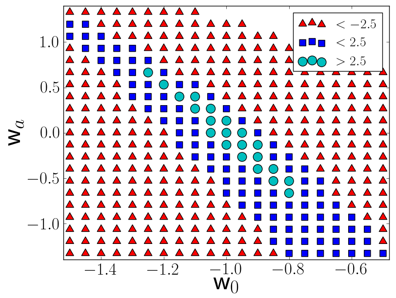
Figure 2: Each point in this $w_{0}$–$w_{a}$ plot is in turn assumed to be the true model, and the Bayes factor of $\Lambda$CDM versus dark energy is calculated at that point. The (green) circles mark the region where $\Lambda\rm CDM$ is preferred, i.e. $\ln B>2.5$; (blue) squares mark the region in which $\Lambda\rm CDM$ is not discounted, i.e. $-2.5<\ln B<2.5$; and the (red) triangles correspond to the region in which evolving dark energy is correctly preferred, i.e. $\ln B<-2.5$.

2.3 Methods for calculating the Bayes factor

Two different approaches are utilised in calculating $\ln B(w_{0},w_{a})$: nested sampling as devised by Skilling (2006); and the Savage–Dickey Density Ratio, first introduced in a cosmological context by Trotta (2007a).

2.3.1 Nested sampling

Any model is defined by a set of cosmological parameters $\bm{\theta}$; for example, $\Lambda\rm CDM$ can be described by $\bm{\theta}=[w_{\rm de},\Omega_{\rm de},\Omega_{\rm m},\Omega_{\rm r},\Omega_{k},\Omega_{\rm b},H_{0},n_{s},\sigma_{8}]$. The values of each of these parameters must be estimated by means of best fit to the data. This can be done using Bayes theorem, as per equation 4,

$$p(\bm{\theta}\mid D,M)=\frac{p(D\mid\bm{\theta},M)p(\bm{\theta}\mid M)}{p(D\mid M)}\,,$$ (4)

with MCMC methods identifying the point in cosmological parameter space at which the posterior $p(\bm{\theta}\mid D,M)$ is maximised [Hobson et al. 2010].

Notice the denominator in equation 4 is the evidence required for the Bayes factor of equation 3. By integrating over all allowed values of this parameter set $\bm{\theta}$ it is possible to calculate the evidence using equation 5; the evidence is therefore the average likelihood over the prior parameter space, thus rewarding models for predictive power.

$$E(M)=p(D\mid M)=\int p(D\mid\bm{\theta},M)p(\bm{\theta}\mid M)d\bm{\theta}\,.$$ (5)

Nested sampling [Skilling 2006] recasts this multi-dimensional evidence integral in 1D by integrating over the prior mass $X$, where $dX=p(\bm{\theta}\mid M)d\bm{\theta}$ and $L$ refers to the likelihood:

$$E=\int_{0}^{1}L(X)dX\,.$$ (6)

The nested sampling algorithm starts by sampling a large number of points from the likelihood surface simultaneously and assigns equal fractions of the total remaining prior mass to each sample. It then proceeds by adding the lowest probability point ($L_{j}$) (whose prior mass is $X_{j}$) to the evidence integral sum:

$$E=\displaystyle\sum\limits_{j=1}^{m}\frac{L_{j}}{2}(X_{j-1}-X_{j+1})\,.$$ (7)

The algorithm then reduces the remaining prior mass, by a statistically estimated amount. The lowest likelihood sample is replaced with a sample randomly selected from the prior, with the sole selection criteria that it be of higher likelihood than the previous. The main challenge in implementing the algorithm is to find a way to carry out this sampling efficiently, a simple approach being ellipsoidal sampling [Mukherjee et al. 2006b] and a more sophisticated approach suitable for multi-modal likelihoods being to partition the points into clusters of ellipsoids [Feroz, Hobson & Bridges 2009].

This entire process is repeated, building up the evidence sum, until the accuracy has reached an acceptable level. At the point of termination the remaining contribution to the evidence integral is added. As this is a numerical estimation, several repeats are done from which the mean and error are extracted. A detailed account of the nested sampling implementation we use is given in Mukherjee et al. (2006b).

Calculations of the Bayes factor are in principle simple using nested sampling. The evidence is calculated by first assuming $\Lambda\rm CDM$ as the true model, then independently by assuming evolving dark energy, when simulating survey data. Unfortunately, due to the very large number of computations required to sample both survey and model parameter spaces, nested sampling is too inefficient to be regarded as practical in full MCMC optimizations. However it is still possible to utilise nested sampling when investigating the $\ln B(-1,0)$ FoM for very basic manual optimizations, e.g. manually altering only one survey parameter at a time.

2.3.2 Savage–Dickey Density Ratio (SDDR)

As the nested sampling algorithm is too slow to be seriously considered for the full scope of model selection optimization that we wish to consider, the Savage–Dickey Density Ratio (SDDR) is investigated. The SDDR is a simplification of the Bayes factor that assumes a less complex model is nested within a more complex model and that the priors are separable. For example, $\Lambda\rm CDM$ is nested within the evolving dark energy model’s parameter space where $w_{0}=-1$ and $w_{a}=0$, and furthermore the priors concerned with these two dark energy parameters ($\bm{w}$) and those concerned with the nuisance parameters ($\bm{N}$) of the models can be separated, i.e. $p(\bm{w},\bm{N})=p(\bm{w})p(\bm{N})$. The SDDR is given by equation 8,

$$B=\frac{p(\bm{w}\mid D)}{p(\bm{w})}\Bigg{|}_{\bm{w}=\bm{w^{*}}}\,,$$ (8)

where $\bm{w^{*}}$ represents the simpler models’ nested values, being a special case of the more complex model’s parameter vector $\bm{w}$. For a derivation of this see Appendix B of Trotta (2007a).

This allows the Bayes factor to be evaluated by considering the marginalised posterior probability of the more complex model and its prior at the parameter values of the nested simpler model. This removes the need for the computationally expensive integral as required to calculate the evidence via equation 5. Both assumptions made in deriving equation 8 are true for the dark energy models under consideration and nothing has been assumed about the likelihood, therefore it is exact in this case. However, we now make a further assumption that makes this implementation approximate.

To minimise alteration to the original DETF optimization and hence calculation time, our SDDR calculation assumes Gaussianity of the posterior in $w_{0}$ and $w_{a}$ having marginalized over all other parameters. The Bayes factor can therefore be forecast with only a few simple additions to the DETF optimization, by application of the following:

$$\centering B(w_{0},w_{1})=\frac{\Delta w_{0}\Delta w_{1}}{2\pi\sqrt{\det F^{-1}}}e^{-\frac{1}{2}\sum_{\mu\nu}(w_{\mu}-w^{*}_{\mu})F_{\mu\nu}(w_{\nu}-w^{*}_{\nu})}\,.\@add@centering$$ (9)

In this equation $\nu$ and $\mu$ can have values of either 0 or 1; $\bm{w^{*}}$ are the nested values of the simpler model; $w_{1}=w_{a}$; $\Delta w_{0}$ and $\Delta w_{1}$ are the width of the flat prior ranges; and $F_{\mu\nu}$ is the marginalised Fisher matrix. A numerical approach using finite-differencing was used to determine the Fisher matrix, the details of which are described in Appendix A of P10.

Recall that values larger than unity ($\ln B>0$) support the simpler model, and values less than unity ($\ln B<0$) support the more complex model. We see then that the pre-factor of equation 9 acts as an amplitude, measuring the ratio of the area of $w_{0}$–$w_{a}$ parameter space allowed by the more complex model to the area of the error ellipse; this term therefore penalises the more complex model for unjustified parameter space. The exponential part measures the distance between the two models and can lend support for the more complex model by suppressing the amplitude term.

This SDDR approach allows investigation of both model selection FoMs. However for the area^-1 FoM to be practical for full MCMC optimizations it needs refining; for example, $\ln B(w_{0},w_{a})$ calculations could be parallellized and MCMC could be used to determine the area^-1.

2.3.3 A note on priors

The prior range mentioned in section 2.2 is the same as that used in M06, but we acknowledge that the choice of priors is arbitrary to a degree. Whilst changing the prior range, i.e. $\Delta w_{0}$ and $\Delta w_{1}$, will quantitatively affect $\ln B$ calculations it will not qualitatively change the FoMs we are considering. Furthermore, as discussed in M06, different (sensible) prior choices will not have a serious impact on the interpretation of the resulting Bayes factors.

2.4 P10 correction

Early in the process of adding the new FoM options to the optimization we became aware of a coding error that made the original results in P10 incorrect. We have fixed this error and present the updated results in Appendix A. The main differences are a reduction in the DETF FoM by a factor of 3 and that the optimization is qualitatively unchanged by including curvature as a nuisance parameter. The latter of these results is found to be also true of the model selection FoMs we investigate in the following, therefore we do not explicitly consider curvature in any of our presented findings.

3 Testing our model selection Figures of Merit

As mentioned, both the nested $\ln B(-1,0)$ and SDDR area^-1 computations are quite slow. To deal with this issue, discrete, i.e. manual, optimizations are considered.

Large-scale surveys such as this are designed with the number of fibres tuned to the required source density, therefore repeated observations of the same area of sky are rarely needed. Furthermore the minimum exposure time is nearly always sufficient to achieve the required S/N on large populations of the the observed galaxies ($\sim$80%) which is why the DETF optimization prefers to maximise the area [Parkinson et al. 2010]. We therefore chose to set the time and area to maximum and then manually vary the maximum and minimum redshift limits. In doing so we have essentially maximised over all other survey parameters, which allows clearer interpretation of the FoM performance.

3.1 $\bm{\ln B(-1,0)}$: an absolute scale for optimization

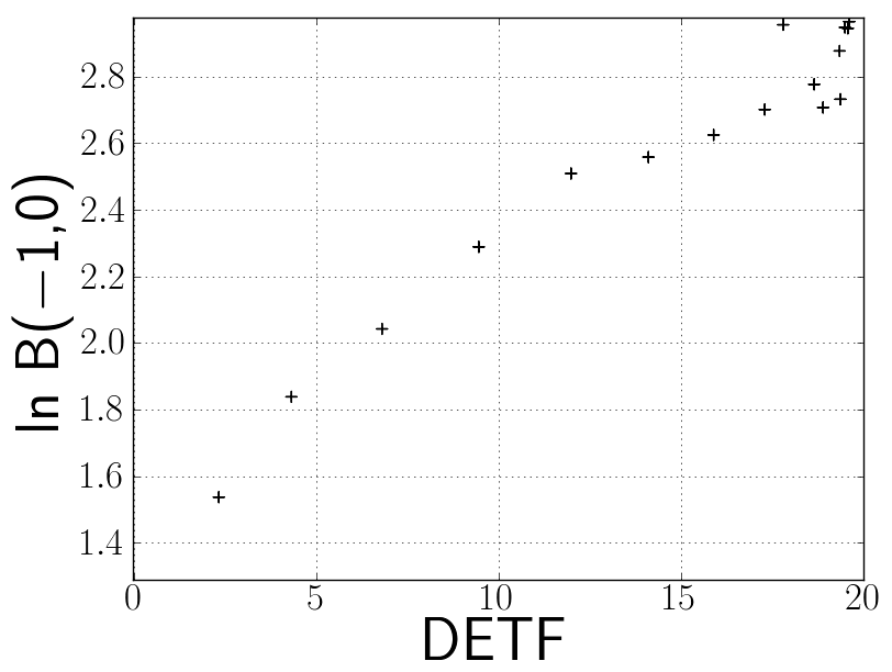
Figure 3: Plot showing the relation between the DETF FoM and the nested $\ln B(-1,0)$ FoM. The monotonic relation between the two is clear, with increased scatter seen around the maximal values.

The findings of our nested sampling discrete optimization are summarised in Figure 3, which compares the behaviour of $\ln B(-1,0)$ with that of the DETF FoM.

The mostly monotonic relation we see between the DETF and the nested $\ln B(-1,0)$ FoMs means that a DETF optimized survey will be extremely similar to one optimized with $\ln B(-1,0)$. However the latter FoM provides an absolute scale; in this case $\ln B(-1,0)$ shows the survey is capable of strongly preferring $\Lambda\rm CDM$ when the DETF FoM for the equivalent survey configuration is still around 60% of its optimum. This additional information would be invaluable when deciding on a survey’s operating mode.

3.2 Gaussian SDDR $\bm{\ln B(-1,0)}$: an immediately viable model selection optimization FoM

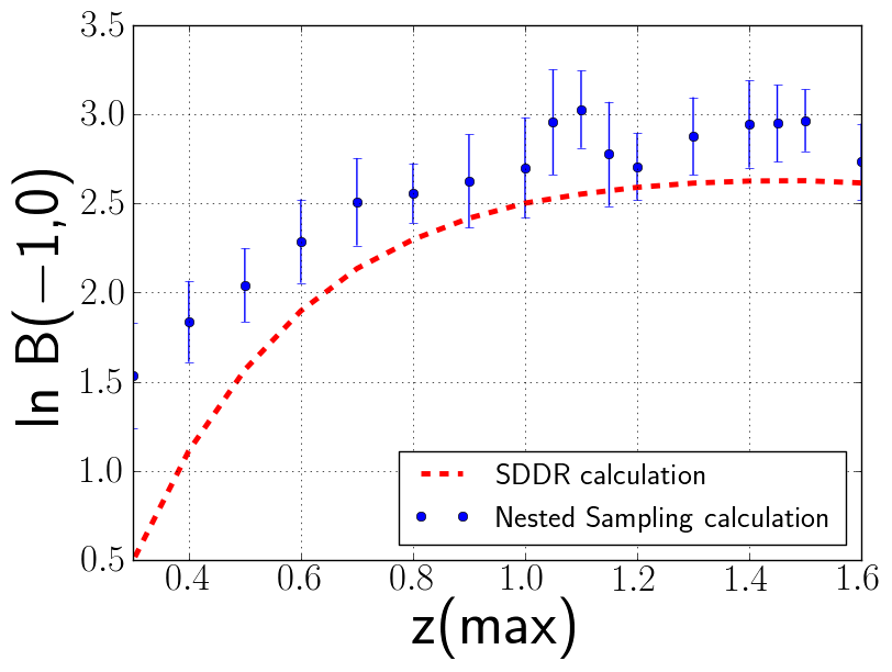
Figure 4: Comparison of the $z_{\rm max}$ dependence of $\ln B(-1,0)$ when calculated with nested sampling and Gaussian SDDR. The (blue) circles mark the nested smapling calculations of $\ln B(-1,0)$, whilst the dashed (red) line shows the respective Gaussian SDDR calculations. The Gaussian SDDR numerically underestimates $\ln B(-1,0)$ in a nearly perfectly uniform fashion. We infer that it would be trivial to calibrate it to the more accurate nested calculations.

By deploying the SDDR Gaussian approximation it is possible to perform full MCMC optimizations with $\ln B(-1,0)$. However, being an approximation it is necessary to establish the impact of this simplification on the resulting Bayes factors. Figure 4 compares the Gaussian SDDR calculations with the more accurate nested sampling ones in the case where the upper redshift limit $z_{\rm max}$ is varied.

We can see that the SDDR $\ln B(-1,0)$ typically underestimates the Bayes factor. While the assumption of Gaussianity has been seen to be good around the peak of the likelihood [Mukherjee et al. 2006a], it appears to be less accurate around the tails. If the information in the tails is overestimated by this assumption, i.e. if in reality the likelihood falls off more sharply than in the Gaussian approximation, then the average likelihood and therefore evidence for the evolving dark energy model will be overestimated. This will result in the underestimation of the Bayes factor we see here. It would also explain the increased scatter away from the monotonic relation between the nested $\ln B(-1,0)$ and the DETF FoM for stronger surveys, clearly seen in Figure 3. More accurate surveys will have tighter likelihood peaks, and therefore any non-Gaussianity of the tails would be more influential.

Despite this, the general trend is the same, best seen by making a logarithmic plot of the DETF FoM against nested calculations of $B$, and writing equation 9 for the Gaussian SDDR calculation of $B$ in terms of the DETF FoM:

$$\ln B_{\rm SDDR}(-1,0)=\ln\left(\frac{\Delta w_{0}\Delta w_{a}}{2\pi}\right)+\ln\left(\rm FoM_{DETF}\right)\,.$$ (10)

Figure 5 shows how the nested calculation of $\ln B(-1,0)$ follows this linear relation well, despite the increased deviations around the highest values. This implementation of SDDR presents a good alternative to the nested sampling approach, and furthermore it is as quick as the DETF optimization with only a few extra calculations required. Its underestimation of the Bayes factor is also seen to be almost uniform across the redshift range of Figure 4, and we therefore infer that it would be simple to calibrate the SDDR FoM to gain more accurate estimates of $\ln B$ by performing a few nested sampling computations of $\ln B$.

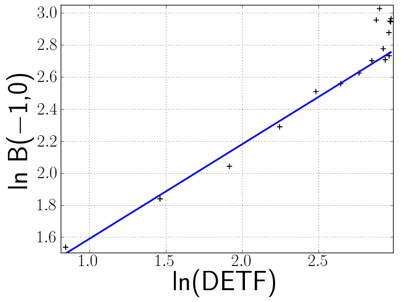
Figure 5: Logarithmic plot of the DETF FoM against the nested $\ln B(-1,0)$ FoM. We see that the nested calculation follows the linear relation described by equation 10.

3.3 Area^-1: an informative optimization FoM with potential for practical application

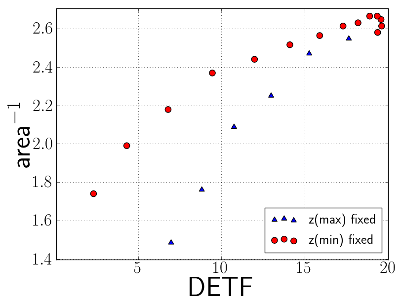
Figure 6: DETF FoM performance compared with that of the area^-1 FoM. The (blue) triangles result from a manual optimization where $z_{\rm min}$ alone is adjusted, and the (red) circles from adjusting $z_{\rm max}$ only. There is a clear monotonic relation between the two, with general agreement around the maximum. FoMs were normalised with respect to their maximum.

The Gaussian SDDR approximation also allows investigation of the area^-1 FoM but, as with the nested calculations of $\ln B(-1,0)$, computational limitations mean that we are again restricted to manual optimizations.

Figure 6 shows the monotonic relation between the area^-1 FoM and that of the DETF. This further supports the widespread adoption of this parameter estimation FoM. The area^-1 FoM is seen to attain a performance only slightly weaker than its optimum while the DETF is only 50% of its optimum. This means that the model selection ability of a survey is close to optimal for much weaker configurations then the DETF optimization would deem acceptable.

3.4 Fixed galaxy density: a faster, accurate approximation

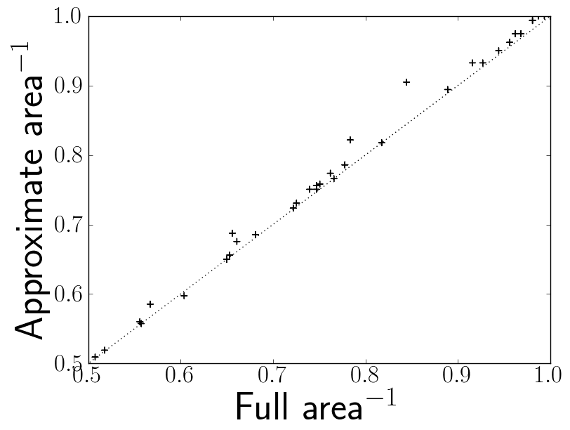
Figure 7: Full implementation area^-1 FoMs plotted against the corresponding values found using the fiducial galaxy approximatation. In both cases the FoMs have been normalised with respect to their maximum. Clearly the approximation is very good.

As the area^-1 FoM is slow to compute we consider a further approximation. We exclude the modelling of the galaxy density, required for the Seo & Eisenstein (2007) transfer function, from the $w_{0}$–$w_{a}$ gridding. That is to say we assume that $\Lambda\rm CDM$ is the true model for all calculations of galaxy density, regardless of the assumed cosmology in calculating the Bayes factor. In doing so we reduce the number of times the galaxy density must be estimated from of order 400 per FoM to 1. There are 10,000 FoM calculations in an average optimization, so this substantially reduces the calculation time.

The results of this are summarised in Figure 7, showing this to be an extremely good approximation and that this FoM is not particularly sensitive to galaxy density. This provides a much faster alternative to the full implementation of the area^-1 FoM.

3.5 FoM performance overview

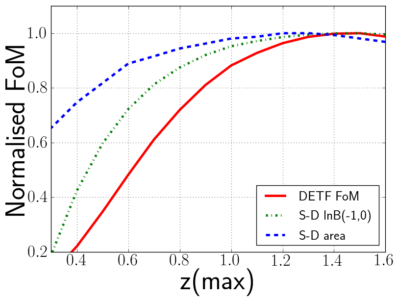
Figure 8: Optimization results comparing the various FoMs investigated. All FoMs were normalised with respect to their maximum values. The (blue) dashed line marks the SDDR area^-1 FoM, the (green) dot-dashed line plots the SDDR $\ln B(-1,0)$ FoM, and the (red) solid line shows the DETF FoM.

Figure 8 provides a summary of this investigation with all FoMs (excluding the nested sampling calculation of $\ln B(-1,0)$) plotted as a function of maximum redshift. From this plot and that of Figure 4 we see that the model selection FoM would deem a maximum redshift of about 0.7 to be acceptable. Clearly a maximum redshift of between 1.1 and 1.6 is optimal using the DETF, but it is not clear how much this upper limit may be reduced before the survey will not fulfil its desired purpose.

Similarly a survey that extends to higher redshifts than 1.6 will be less than optimal but will, up to a point, be deemed suitable for its purpose by both model selection FoMs. This highlights the value of this approach as our modelled survey has the capability to push to higher redshifts; such high-redshift observations are extremely useful for ancillary cosmology and astronomy. The model selection optimizations provide well informed flexibility of this upper $z$ limit.

The absolute scale of $\ln B(-1,0)$ and the additional information from area^-1 are very useful when considering time allocations. For example, a dark energy survey will have limited time on a telescope; being able to provide detailed information on the required time would be vital for requesting more time be allocated, or when sharing an overall allocation between different independent observation modes within the same project.

As the FoM have all been seen to have a monotonic relation, information from DETF and $\ln B(-1,0)$ optimizations can be used to perform similar discrete area^-1 optimizations as done here, with negligible expense of time and effort.

4 Application to spectroscopic BAO surveys

4.1 Optimising SuMIRe PFS for model section ability

We now apply the model selection FoMs that have been investigated so far to a practical optimization. To make this as relevant as possible we update the original P10 survey parameters to be as close as can be to SuMIRe PFS. This involves increasing the mirror diameter from 8m to 8.2m and the fibre diameter from 1 arcsec to 1.2 arcsecs, while the target signal-to-noise ratio and throughput are slightly reduced from the original. The specifications for the survey we optimize in this section are given in Table 4; otherwise the survey details remain unchanged from our original optimization as summarised in Table 1. For a full description of SuMIRe PFS see Takada & Silverman (2010).

Parameter	SuMIRe specification
mirror diameter	8.2m
fibre diameter	1.2 arcsec
aperture	0.8
Signal/Noise	6.5
Number of fibres	3000
Field of View	$9\pi/16$ sq.deg.

Table 4: The SuMIRE specification used in our calculations.

As the WiggleZ survey is complete and BOSS (Baryon Oscillation Spectroscopic Survey) is well under way, the SuMIRe optimization must concentrate on filling the available observational niche, otherwise some of its allocated time will be lost on unnecessary repetition of observations. With this in mind we include the forecast data-points for BOSS and WiggleZ as prior information for this optimization.

Although we have so far only considered the redshift range 0.1 to 1.6, SuMIRe PFS as modelled here is capable of observing redshifts up to about 4.9. At redshifts greater than 2 the spectrograph can measure the Lyman-alpha spectral features, however for $1.6<z<2$ there exists an effective blind spot in which no spectral features are observable by this survey. This optimization therefore considers two independent redshift mega-bins; the low-redshift mega-bin covering $0.1<z(\rm low)<1.6$ and the high-redshift mega-bin covering $2<z(\rm high)<4.9$. Figure 9 depicts the mega-bin modelling and Table 5 details the survey variables. The modelling details of the high redshift mega-bin can be found in P10.

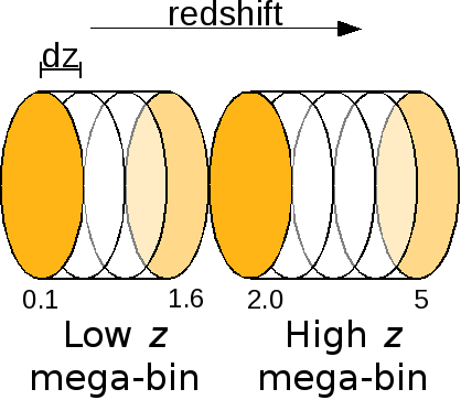
Figure 9: Representation of the $z$ binning method used in optimizing SuMIRe PFS.

Survey Parameter	Symbol (mega-bin)
Time split between mega-bins	$\tau$(low), $\tau$(high)
Area covered	$A$(low), $A$(high)
Minimum of redshift mega-bin	$z_{\rm min}$(low), $z_{\rm min}$(high)
Maximum of redshift mega-bin	$z_{\rm max}$(low), $z_{\rm max}$(high)
Number of pointings	$n_{\rm p}$(low), $n_{\rm p}$(high)

Table 5: Survey parameters varied in the SuMIRe optimization.

Two types of optimization are performed. Firstly a full MCMC optimization using the Savage–Dickey $\ln B(-1,0)$ FoM is executed using 3 different optimization settings:

1. Varying all 10 survey parameters listed in Table 5, i.e.  $\tau$, $A$, $z_{\rm min}$, $n_{\rm p}$ and $z_{\rm max}$ over both redshift mega-bins,

2. Focusing all time in the low-redshift mega-bin, i.e. varying only $A$(low), $z_{\rm min}$(low), $n_{\rm p}$(low) and $z_{\rm max}$(low),

3. Focusing all time in the high-redshift mega-bin, i.e. varying only $A$(high), $z_{\rm min}$(high), $n_{\rm p}$(high) and $z_{\rm max}$(high).

From optimization (i) we establish the optimum time split between the low and high mega-bins; the optimum redshift and exposure times for each are then found from (ii) and (iii). Discrete optimizations can then be performed with the Savage–Dickey area^-1 FoM. To do this we fix the redshift limits and exposure time according to the $\ln B$ optimization results. By manually varying the time (and therefore area) we can examine this FoM’s performance with total time allocation and its split across the redshift mega-bins.

The SuMIRe project has moved on a great deal from the version modelled here, for example the current design has no redshift blind spot and can in principle observe as deep as $z=10$ if targets are available [Murayama 2011]. As such direct comparison cannot be drawn; we instead use the observational technique outlined in the 2010 SuMIRe PFS white paper [Takada & Silverman 2010] as our reference. In this set-up the survey only covers an area of 2000 sq.deg., limited by the projected area that the Hyper Suprime-Cam (HSC), needed for pre-selecting PFS’s target galaxies, will cover during its operational lifetime. Its redshift range is 0.6 to 1.6, exposure time is 15 minutes, and therefore total time is roughly 500 hours.

4.2 Optimal performance for preferring $\bm{\Lambda\mathrm{CDM}}$ achieved with all time spent observing redshifts between 0.1 and 1.6

The full MCMC optimization using $\ln B(-1,0)$ found that an improvement in our confidence in $\Lambda\rm CDM$ (if it is the underlying model) will be gained for a wide range of time allocation to the low redshift mega-bin, but it is clearly preferable to focus all time in this mega-bin. This is summarised in Figure 10, plotting $\tau_{\rm low}$ against $\ln B(-1,0)$.

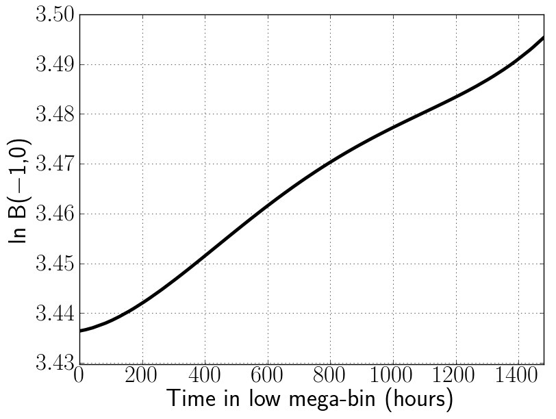
Figure 10: Plot of the time allocation in the low mega-bin versus the $\ln B(-1,0)$ FoM; this results from varying all parameters in both redshift mega-bins, i.e. optimization setting (i). Note, any remains of the total 1500 hours is allocated to the high redshift mega-bin. Allocating all 1500 hours to the low mega-bin is seen to be preferable

Figure 11 shows how the value of $z_{\rm min}(\rm low)$ affects the survey’s ability to prefer $\Lambda\rm CDM$. We find that it is best to make use of the full redshift range in the low mega-bin, i.e. $0.1<z<1.6$. However, as long as the lower limit is not greater than $z=1.0$ there is no great loss of performance. This has a great deal to do with the fact that the data-points measured by WiggleZ and BOSS cover the redshift range between 0.1 and 1.0. It also indicates that the reference survey’s choice of $z_{\rm min}=0.6$ is reasonable.

As with the DETF optimization there is a preference for maximising the survey volume, and we therefore find that the optimal survey minimises the exposure time and maximises survey area.

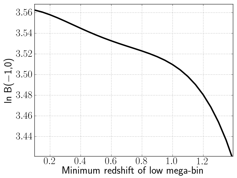
Figure 11: Plot of the minimum redshift of the low mega-bin versus $\ln B(-1,0)$ when all time is focused in the low mega-bin; this results from varying all parameters in both redshift mega-bins, i.e. optimization setting (i). $z_{\rm min}=0.1$ is seen to be preferable, with model selection performance dropping off steeply after $z_{\rm min}=1.0$

4.3 For optimal dynamical model selection ability, total time of over 1100 hours is preferable, with a minimum of 500 hours spent in the low-redshift regime

The time-area^-1 FoM plots of Figures 12 and 13 summarise the findings of our discrete area^-1 optimization used to investigate the optimal time split. Their jagged nature is a result of a tipping-point style effect caused by the gridding approach we use for investigating the dark energy parameter space. This jaggedness is absent in Figures 6 and 8 because the range for the FoM is greater by a factor of around 4. An MCMC style approach to measuring the area^-1 would produce more gradual increase of this FoM. The flat-lining should be conceptually smoothed across, joining the tips of the jags.

Note that in making the total time plot of Figure 12, four different time splits are calculated per total time allocation; it was found the maximal survey spends all the time in the low mega-bin regardless of the total time allocated.

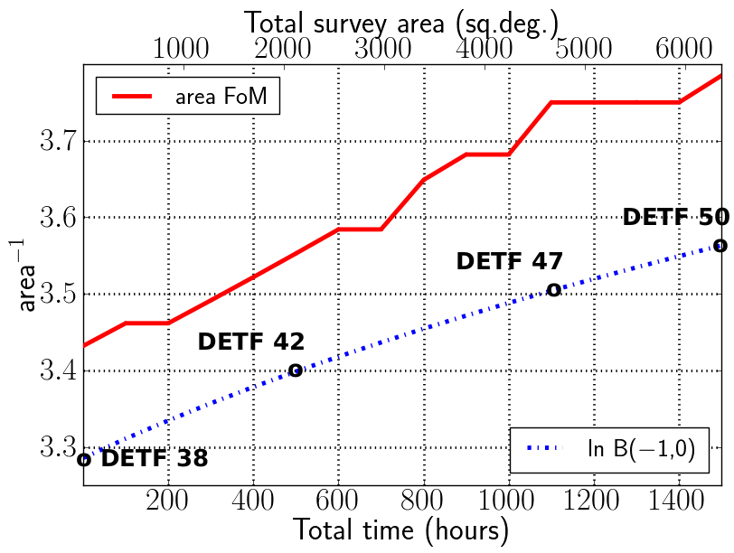
Figure 12: Plot of the total time allocation effect against the Area^-1 FoM; this is achieved by fixing the redshift range at 0.1 - 1.6 and exposure time to 15 minutes. We see that optimal results can be achieved for time allocations above 1100 hours.

The main thing we note is the very limited gain in carrying out this survey with 500 hours as per our reference survey; $\ln B(-1,0)$ increases from 3.3 to only 3.4, and the prior-space area in which $\Lambda\rm CDM$ cannot be ruled out, i.e. area in which $\ln B>-2.5$, reduces from 30% to only 29%. This fact is already clear from the DETF FoM with an increase of only 4. From our model selection optimization a time allocation of around 1100 hours is best with a minimum of 500 hours spent in the low mega-bin, but even this promises only a minimal advance in our knowledge.

SuMIRe PFS as modelled here is only a part of the SuMIRe project; the other part being the HSC survey, which we’ve mentioned is used to pre-select galaxies for PFS. Having the pre-selection survey as an integral part of the project, operating on the same telescope, is of great benefit in itself, but the HSC will also be used to measure gravitational lensing. Dark energy constraints from BAO and gravitational lensing are complementary and as such their combination dramatically boosts the power of SuMIRe. This is clear from the white paper’s forecasted DETF FoMs which rise from 33 (for both PFS and BOSS surveys), to 217 when the HSC survey is included (i.e. PFS, BOSS and HSC). Again SDSS and Planck datasets were taken as prior information in calculating these FoMs [Takada & Silverman 2010].

It is a pity our modelled survey is not as comprehensive as the full incarnation of SuMIRe, as the model selection FoM’s benefits would be more transparent; we therefore present this section as a proof of concept rather than a display of strength.

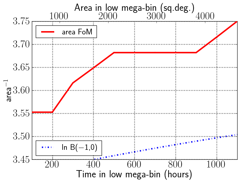
Figure 13: Plot of time allocation in the low mega-bin versus the Area^-1 FoM; this is achieved by fixing the redshift range at 0.1 - 1.6 and exposure time to 15 minutes. Any remains from the total 1100 hours are allocated to the high redshift mega-bin. We see that spending over 500 hours in the low is preferable for optimal model selection ability.

5 Conclusions

We have discussed the importance of survey optimization, particularly in finding the appropriate niche for an upcoming survey. The usual approach of parameter estimation, which maximises the survey’s ability to accurately measure the parameters of interest, assumes that a particular model is true thereby ignoring the model selection requirement of these surveys. A future survey’s primary aim is to discount models with the ultimate goal of one to prevail. We therefore attempt to directly optimize a survey for its intended purpose, model selection.

In doing so we test Bayesian model selection in the context of optimizing a ground-based spectroscopic baryon acoustic oscillation survey. To do this we extend an optimization based on the DETF FoM, designing it to instead target two Bayesian FoMs. For the sake of efficiency we assume a Gaussian likelihood in both cases. The results of each one’s optimization are compared with that of the original parameter estimation FoM.

The $\Lambda\rm CDM$ Bayes factor, $\ln B(-1,0)$, measures the survey’s ability to prefer $\Lambda\rm CDM$ if it does transpire to be the correct model. This quantifies the increase in probability of one model over another in light of fresh data, assuming $w_{0}=-1$ and $w_{a}=0$ for all calculations.

For a second FoM, which we call area^-1, the dark energy parameter space is gridded and discrete calculations of $\ln B(w_{0},w_{a})$ are made for each point on the grid. For each of these calculations the $w_{0}$, $w_{a}$ values for that point in parameter space are assumed. The area in which $\Lambda\rm CDM$ was not discounted when presumed incorrect, i.e. all places where $\ln B(w_{0},w_{a})>-2.5$, was calculated. The smaller this area, the more effective a survey is at model selection and its inverse forms our second FoM.

The $\ln B(-1,0)$ FoM is implemented with only minor adjustment to the original optimization, and furthermore the calculation time is unchanged. Whilst this FoM follows the same trend as the original, and therefore its optimal survey agrees, it does enjoy the added merit of being an absolute scale allowing interpretation of when the survey is ‘good enough’. This added insight is invaluable for making efficient use of precious survey time or when bidding for extra time allocations. It also allows for educated flexibility, essential for adding independent science goals to a project.

The area^-1 FoM needs some further development to be useful in full MCMC optimizations, but even as presented here it has potential for immediate application. We again find this FoM follows the trends of the original optimization, as such the resulting optimal surveys will be very close. However there is more information to be had using this model selection approach; where the other FoMs increase gradually in a near linear fashion before reaching a brief peak, the area^-1 FoM is seen to reach values close to optimum for configurations the usual approach would deem relatively weak. This approach provides better insight into the flexibility of the survey’s observational strategy.

Whilst these results do not blow the usual parameter estimation approach out of the water, they do present a powerful alternative. Considering the extreme simplicity with which the $\ln B(-1,0)$ FoM can be implemented it seems wasteful to not at the very least calculate this alongside the DETF FoM. As mentioned the area^-1 FoM also has potential for immediate application even before improvements such as MCMCing the area or parallelising are considered. Whilst there might not always be a strong trend such as the need to maximise survey volume to allow the fixing of everything but time, there will invariably be refined optimizations for which the discrete method used here is applicable.

Dark energy surveys often require several probes be exploited, some requiring different observational strategies; for example, the Dark Energy Survey has one operational mode for taking supernovae data, and another for everything else [Annis et al. 2004]. These Bayesian FoMs are perfect for identifying the best time share between such observational modes, ensuring each independent survey mode is good enough to achieve its design goals.

The Gaussian approach used here is seen to be reasonable for the $\ln B(-1,0)$ FoM. We do not however investigate its impact on the area^-1 FoM, which requires future work as the assumption will be less appropriate away from the fiducial point in dark energy parameter space. However it seems unlikely that the general trend will be severely altered, and as such development to improve the speed of our implementation would be beneficial.

Despite the fact we have focused on a particular survey, the methods discussed here are applicable to any dark energy optimization; furthermore this can, in theory, be employed beyond dark energy surveys and even cosmology itself. Therefore it will be interesting to see how such FoMs fare under different circumstances, especially in cases where an absolute scale is of particular use, as is the case for multi-probe surveys.

Appendix A Revision of P10 results

The optimal survey parameter values found with the debugged version of the optimization are summarised in Figure 14 and Table 6. The most pronounced difference compared with P10 is the reduction of performance predicted by this optimization, with returned FoMs around a factor of 3 smaller. This has impact on the forecasted fitness of this survey, which at the time of P10’s publishing performed fairly well alongside its competitors. These results show it would not have been as strong as previously thought.

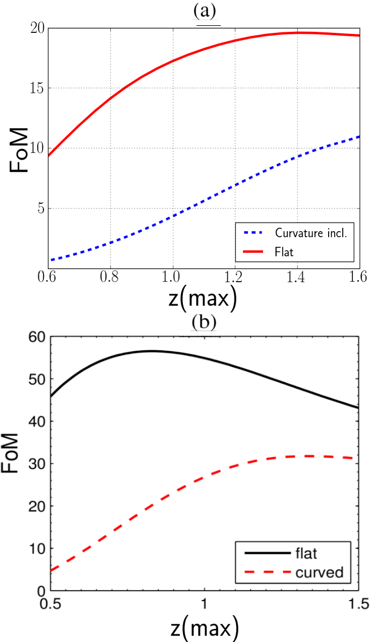
Figure 14: (a) Revised $z_{\rm max}$ - DETF FoM relation when the universe is assumed flat (red solid line) compared to when curvature is included (blue dashed line) (b) Original $z_{\rm max}$ - DETF FoM relation when the universe is assumed flat (black solid line) compared to when curvature is included (red dashed line). [Lower image from P10.]

Survey Parameter	Flat	Curved
$A_{\rm low}$(sq.degs)	6300	6300
$\tau_{\rm low}$ (hours)	1500	1500
$z_{\rm min}(\rm low)$	0.1	0.1
$z_{\rm max}(\rm low)$	1.5	1.6
exposure time (mins)	15.0	15.0
number density (low) $\rm(h^{3}/Mpc^{3})$	$5.2\times 10^{-4}$	$4.4\times 10^{-4}$
number of galaxies (low)	$4.8\times 10^{8}$	$4.6\times 10^{8}$
FoM	20	11
Unoptimized FoM	7	3

Table 6: Revised optimal survey parameters obtained with the debugged version of the WFMOS optimization.

The improvement in performance achieved by carrying out optimization is around a factor of 3 in both the original and debugged results, this is seen by comparison with the unoptimized FoMs. There is also general agreement that including curvature degrades the FoM, due to presence of an extra parameter in the Fisher matrix diluting constraining power on the dark energy parameters.

In the original results, it was inferred that a gamble exists in the assumption of flatness. P10 found that to proceed with the flat optimization settings, i.e. limiting observation to $0.1<z<0.7$, would be damaging if curvature does in fact require constraining. However the new results find far less of a clash of interests, with the inclusion of curvature pushing the upper redshift limit up from 1.5 to only 1.6. This is best quantified in Table 7 where the two different optimal survey configurations are tested under the opposite cosmological assumption. This is achieved by calculating the FoM with curvature included, with the survey configuration fixed according to the results of the flat optimization, and vice versa.

	Flat opt.	Curv opt.
	$z_{\rm range}=0.1$–$1.5$	$z_{\rm range}=0.1$–$1.6$
FoM (assuming flat)	20	18
FoM (Curvature incl.)	10	11

Table 7: Revised results of degradation caused by either not accounting for curvature in optimization when it is necessary or allowing for it when it is not. For all configurations the area is set to 6300 and the time in the low to 1500.

Clearly there is little difference in the performance of the two different optimization results if curvature does need to be considered, whereas in the previous result, the flat optimal survey achieved a FoM about 50% poorer than that of the curvature included optimal survey.

It is worth noting that although the curvature-included optimal survey spends all time in the low mega-bin, it was found that there is no loss in spending up to 380 hours in the upper redshift band, providing that the lower limit is 2.0 and the upper no less that 3.5. This can be seen in Figure 15 which shows the dependence of the FoM on $z_{\rm min}$ and $z_{\rm max}$ in the high redshift mega-bin. Furthermore when this survey configuration is tested with flatness assumed, the FoM is 17, so there is still no serious impact on the power of the survey if considering curvature transpires to be unnecessary. This is a positive feature, as it is likely that non dark energy science would benefit greatly from such time allocation; its presence could have potentially increased support for this project.

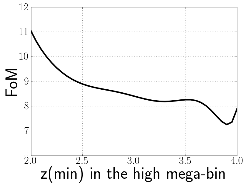
(a) $z_{\rm min}(\rm high)$

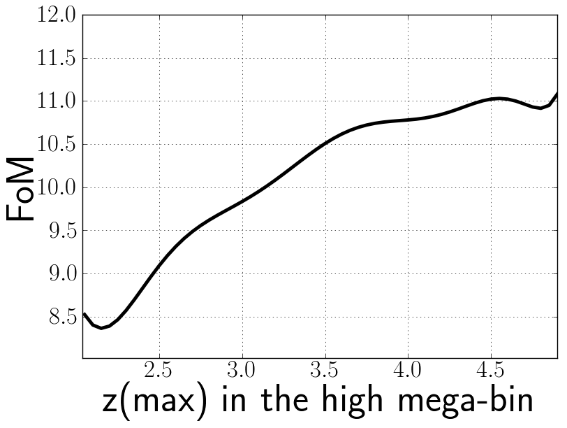
(b) $z_{\rm max}(\rm high)$

Figure 15: The $z$ range sensitivity when 380 hours assigned to high-redshift mega-bin. (a) Shows how the DETF FoM varies with $z_{\rm min}(\rm high)$, and (b) shows how the DETF FoM varies with $z_{\rm max}(\rm high)$. The lack of sensitivity indicates that time spent in the upper mega-bin is not vital, but is also not damaging providing the upper redshift limit is greater than $\sim$3.6 and the lower 2.0.

References

- [Albrecht et al. 2006] Albrecht A. et al., 2006, astro-ph/0609591
- [Albrecht et al. 2009] Albrecht A. et al., 2009, arXiv:0901.0721
-
[Annis et al. 2004]
Annis J. et al., 2004, available
from:
https://des.fnal.gov/main_documents/A_Proposal_to_NOAO.pdf - [Bassett 2005] Bassett B. A., 2005, Phys. Rev., D71, 083517, astro-ph/0407201
- [Bassett, Nichol & Eisenstein 2005a] Bassett B. A., Nichol R. C., Eisenstein D. J., 2005a, Astron. Geophys, 46, 526, astro-ph/0510272
- [Bassett, Parkinson & Nichol 2005b] Bassett B. A., Parkinson D., Nichol R. C., 2005b, ApJ, 626, L1, astro-ph/0409266
- [Caldwell & Kamionkowski 2009] Caldwell R. R., Kamionkowski M., 2009, Ann. Rev. Nucl. Part. Sci, 59, 397, arXiv:0903.0866
- [Chevallier & Polarski 2001] Chevallier M., Polarski D., 2001, Int. J. Mod. Phys., D10, 213, gr-qc/0009008
- [Cox 1946] Cox R. T., 1946, Am. J. Phys., 14, 1, 1
- [Feroz, Hobson & Bridges 2009] Feroz F., Hobson M. P., Bridges M., 2009, MNRAS, 398, 1601, arXiv:0809.3437
- [Gregory 2005] Gregory P., 2005, Bayesian Logical Data Analysis for the Physical Sciences, Cambridge University Press
- [Hastings 1970] Hastings, W. K., 1970, Biometrika, 57 97
- [Hobson et al. 2010] Hobson M., Jaffe A. H., Liddle A. R., Mukherjee P., Parkinson D., 2010, Bayesian Methods in Cosmology. Cambridge University Press
- [Jaynes 2003] Jaynes E. T., 2003, Probability Theory: The Logic of Science, Cambridge University Press
- [Jeffreys 1961] Jeffreys H., 1961, Theory of Probability, 3rd edition, Oxford University Press
- [Kass & Raftery 1995] Kass R. E., Raftery A. E., 1995, JASA, 90, 430, 773
- [Linder 2003] Linder E. V., 2003, Phys. Rev. Lett., 90, 091301, astro-ph/0402503
- [MacKay 2003] MacKay D. J. C., 2003, Information theory, inference and learning algorithms, Cambridge University Press
- [Metropolis et al. 1953] Metropolis, N., Rosenbluth, A. W., Rosenbluth, M. N., Teller, A. H., Teller, E., 1953, J. Chem. Phys. 21, 1087
- [Mukherjee et al. 2006a] Mukherjee P., Parkinson D., Corasaniti P. S., Liddle A. R., Kunz M., 2006a, MNRAS, 369, 1725, astro-ph/0512484
- [Mukherjee et al. 2006b] Mukherjee P., Parkinson D., Liddle A. R, 2006b, ApJL, 638, L51, astro-ph/0508461
-
[Murayama 2011]
Murayama H., 2011, available from:
http://hitoshi.berkeley.edu/misc/LAM%20May%202011.pdf - [Parkinson et al. 2009] Parkinson D., Blake C., Kunz M., Bassett B. A., Nichol R. C., Glazebrook K., 2009, MNRAS, 377, 185, astro-ph/0702040
- [Parkinson et al. 2010] Parkinson D., Kunz M., Liddle A. R., Bassett B. A., Nichol R. C., Vardanyan M., 2010, MNRAS, 401, 2169, arXiv:0905.3410 [P10]
- [Schlegel et al. 2011] Schlegel D. et al., 2011, arXiv:1106.1706
- [Seo & Eisenstein 2007] Seo H., Eisenstein D. J., 2007, ApJ, 665, 14, astro-ph/0701079
- [Skilling 2006] Skilling J., 2006, Bayesian Anal., 1, 833
-
[Takada 2010]
Takada M., 2010, available from:
www.naoj.org/Projects/newdev/ws10/files/sumire_sep10_takada.pdf -
[Takada & Silverman 2010]
Takada M., Silverman
J. D., 2010, available from:
http://www.naoj.org/Projects/newdev/ws10/files/whitepaper_sumire.pdf - [Trotta 2007a] Trotta R., 2007a, MNRAS, 378, 72, astro-ph/0504022
- [Trotta 2007b] Trotta R., 2007b, MNRAS, 378, 819, astro-ph/0703063
- [Trotta 2011] Trotta R., Kunz M., Liddle A. R., 2011, MNRAS, 414, 2337, arXiv:1012.3195