Range separated functionals in the density functional based tight binding method: Formalism

Abstract

A generalization of the density-functional based tight-binding method (DFTB) for the use with range-separated exchange-correlation functionals is presented. It is based on the Generalized Kohn-Sham (GKS) formalism and employs the density matrix as basic variable in the expansion of the energy functional, in contrast to the traditional DFTB scheme. The GKS-TB equations are derived and appropriate integral approximations are discussed in detail. Implementation issues and numerical aspects of the new scheme are also covered.

1 Introduction

Over the last two decades the density functional based tight-binding (DFTB) method found widespread use in such different areas as computational chemistry, condensed matter physics, biophysics and the ever growing field of nanoscience. DFTB is an approximate density functional theory (DFT) that is characterized by a simplified energy functional and additional integral approximations. These modifications give rise to a highly reduced computational cost maintaining at the same time a useful accuracy for many applications. Starting with the work of Seifert [1], the original DFTB formalism has been generalized in multiple directions. The group of Thomas Frauenheim has been particularly active in this respect. Examples are the self-consistent extension of DFTB [2], the treatment of spin-polarized systems [3, 4] a nd van der Waals interactions [5], the combination with the non-equilibriums Greens function theory in quantum transport [6], or the extension to time dependent DFT(B) [7, 8, 9] and the GW formalism of many body perturbation theory [10].

A general feature of DFTB is that it often parallels the accuracy of DFT for different problem classes, inheriting also spectacular failures of the latter. A large number of these problematic cases can be traced back to the self-interaction error (SIE) of popular local or semi-local exchange-correlation (xc) functionals[11]. In Hartree-Fock (HF) theory the interaction of an electron with itself is exactly canceled by opposite terms in the exchange part of the Fock matrix. As exchange is approximated in the local density or gradient corrected approximations for the xc potential, there is a residual self-interaction. This leads to wrong asymptotics of the Kohn-Sham potential and an overly broadened density [12, 13]. Signatures of this deficiency are seen in such different areas as the incorrect dissociation of radical cations [14], the instability of polaronic defects [15], the incorrect description of organic-metal interfaces [16, 17] or the underestimation of charge transfer excited states [18, 19]. In the field of molecular electronics the self-interaction error has also been found to contribute strongly to the significant overestimation of conductances [20, 21].

In recent years so called range-separated or long-range corrected [22, 23, 24, 25, 26, 27] xc functionals have been found to alleviate the above mentioned difficulties. Going back to Gill [22] and Savin [23], the idea is to split the electron-electron interaction into short-range (sr) and long-range (lr) contributions

$$\frac{1}{r_{12}}=\frac{1-\text{erf}(\omega r_{12})}{r_{12}}+\frac{\text{erf}(\omega r_{12})}{r_{12}},$$ (1)

where the long range part is treated exactly, while the short range part gives rise to a modified pure density functional. In Eq. (1), the term “erf” denotes the error function and $\omega$ is an empirical parameter. The resulting theory may be viewed as a generalization of the well known hybrid functionals [28] with fixed weighting coefficients of density functional and HF exchange. In this way, the error compensation of density functionals for exchange and correlation is kept in the short range, whereas the self-interaction error is removed at least asymptotically through the long range contribution.

Here it should be noted that in the range-separated functionals optimized for solid-state systems, it is often the short-range part that is treated exactly, whereas the long-range part is treated as a density-functional. Such methods allow for an accurate description of fundamental band gaps [29, 30, 31] and avoid the known artefacts of HF exchange for metallic solids [32]. Since we are mostly interested in the improvement of DFTB for finite nanostructures and molecules, we keep with the separation of Eq. 1 in the following. Note also that both range-separated and hybrid methods belong to the Generalized Kohn-Sham (GKS) [33] scheme, as both contain a non-local potential (i.e. a fraction of the non-local HF exchange operator) in the single particle equations.

Several applications and modification of the original subdivision in Eq. 1 have emerged in the past years and show that optimized range separated functionals not only alleviate the above-mentioned problems but also compete with the best hybrid functionals in terms of standard applications like structure prediction and thermochemistry [14, 34]. Moreover it must be underlined that only functionals which contains a full HF contribution in the long-range can correctly describe charge-transfer excited states [35, 36, 37].

The goal of this investigation is to extend the theoretical foundations of the DFTB scheme, currently limited to local or semi-local xc-functionals, to range-separated functionals. The corresponding modified energy functional is presented in section (2), while in section (3) effective GKS equations are derived. Sections (4) and (5) deal with additional approximations for the derived terms in the spirit of the traditional DFTB scheme. The paper closes with a brief summary and outlook.

2 Total energy expression

In the GKS [33] formalism the total energy $E_{\text{tot}}$ can be rewritten as a functional of the density matrix

$$\gamma(\vec{r}_{1},\vec{r}_{2})=2\sum_{i}^{N/2}\psi_{i}(\vec{r}_{1})\psi_{i}^{*}(\vec{r}_{2}),$$ (2)

which equals the electron density $\rho(\vec{r})$ on the diagonal, i.e. $\rho(\vec{r})=\gamma(\vec{r},\vec{r})$. The wave functions $\psi_{i}$ denote the spatial part of GKS spin-orbitals and we confine the treatment to the special case of closed shell systems with $N$ electrons and $N/2$ occupied orbitals. We thus have:

$$E_{\text{tot}}[\gamma]=T[\gamma]+E_{\text{xc}}[\gamma]+E_{\text{H}}[\rho]+E_{\text{ext}}[\rho]+E_{\text{NN}}$$ (3)

where

$$T[\gamma] = \int\left.\left(-\frac{1}{2}\vec{\nabla}_{r_{2}}^{2}\right)\gamma(\vec{r}_{1},\vec{r}_{2})\right|_{\vec{r}_{2}=\vec{r}_{1}}\,d\vec{r}_{1}$$ (4)

$$E_{\text{H}}[\rho] = \frac{1}{2}\iint\frac{\rho(\vec{r}_{1})\rho(\vec{r}_{2})}{r_{12}}\,d\vec{r}_{1}d\vec{r}_{2}$$ (5)

$$E_{\text{ext}}[\rho] = \int\rho(\vec{r})v^{\text{ext}}(\vec{r})\,d\vec{r}$$ (6)

$$E_{\text{NN}} = \frac{1}{2}\sum_{AB}\frac{Z_{A}Z_{B}}{\left|\vec{R}_{A}-\vec{R}_{B}\right|}$$ (7)

represent the kinetic, Hartree, external and nuclear-repulsion energy, respectively. In the range-separated formalism the exchange is divided into a short-range (xsr) and long-range (xlr) contribution and the xc energy functional reads:

$$E_{\text{xc}}[\gamma]=E_{\text{xsr}}[\rho]+E_{\text{xlr}}[\gamma]+E_{\text{c}}[\rho]$$ (8)

where the xlr exchange is given explicitly as a functional of the density matrix

$$E_{\text{xlr}}[\gamma]=-\frac{1}{4}\iint\frac{\text{erf}\left(\omega r_{12}\right)}{r_{12}}\gamma(\vec{r}_{1},\vec{r}_{2})\gamma(\vec{r}_{2},\vec{r}_{1})\,d\vec{r}_{1}d\vec{r}_{2}.$$ (9)

Note that in the GKS formalism the auxiliary system of partially-interacting electron is still described by a single-Slater determinant [33], thus only the exchange is range-separated. The whole electron-electron interaction is range-separated in the the multi-determinant extension of the Kohn-Sham theory [38, 39]. As we are aiming at an approximate scheme that is foremost self-interaction free, it is sufficient to remain in the GKS scheme and to employ local or gradient corrected approximations for the correlation. Explicit functional forms of the $\omega$-dependent short-range exchange for the LDA and the Perdew-Burke-Ernzerhof density functionals are available in the literature [26, 40, 41]. Please note that the special form of the interaction kernel $\text{erf}(\omega r)/r$ in Eq. (9) is not without alternative. Besides the error function also Yukawa and other screened potentials have been used to define interaction ranges. It turns out that the precise choice of the separation function is of minor importance [27]. From a numerical point of view, the form of Eq. (9) is advantageous both for basis functions of Gaussian type or calculations using plane waves, since it allows for an efficient evaluation of the required two-electron integrals.

As the first approximation we now expand the total energy of Eq. (3) around a certain reference density matrix $\gamma_{0}(\vec{r}_{1},\vec{r}_{2})$ up to second order in $\Delta\gamma=\gamma-\gamma_{0}$:

$$E_{\text{tot}}=E^{\text{(0)}}+E^{\text{(1)}}+E^{\text{(2)}}+{\cal O}(\Delta\gamma^{3}),$$ (10)

which parallels the expansion in terms of the density in the conventional DFTB scheme. The individual terms in Eq. (10) are given as:

$$E^{\text{(0)}} = T[\gamma_{0}]+E_{\text{ext}}[\rho_{0}]+E_{\text{H}}[\rho_{0}]+E_{\text{xc}}[\gamma_{0}]+E_{\text{NN}}$$ (11)

$$E^{\text{(1)}} = \int\left.\left(-\frac{1}{2}\vec{\nabla}^{2}_{{\bf r}_{2}}(\vec{r}_{2})\right)\Delta\gamma(\vec{r}_{1},\vec{r}_{2})\right|_{\vec{r}_{2}=\vec{r}_{1}}\,d\vec{r}_{1}$$ (12)

$$+ \int v^{\text{ext}}(\vec{r})\Delta\rho(\vec{r})\,d\vec{r}$$

$$+ \iint\frac{\rho_{0}(\vec{r}_{2})\Delta\rho(\vec{r}_{1})}{r_{12}}\,d\vec{r}_{1}d\vec{r}_{2}$$

$$+ \iint\left.\frac{\delta E_{\text{xc}}[\gamma]}{\delta\gamma(\vec{r}_{1},\vec{r}_{2})}\right|_{\gamma=\gamma_{0}}\Delta\gamma(\vec{r}_{1},\vec{r}_{2})\,d\vec{r}_{1}d\vec{r}_{2}$$

$$E^{\text{(2)}} = E_{\text{H}}[\Delta\rho]+\frac{1}{2}\iiiint\left.\frac{\delta^{2}E_{\text{xc}}[\gamma]}{\delta\gamma(\vec{r}_{1},\vec{r}_{2})\delta\gamma(\vec{r}_{3},\vec{r}_{4})}\right|_{\gamma=\gamma_{0}}\$$ (13)

$$\times \,\Delta\gamma(\vec{r}_{1},\vec{r}_{2})\Delta\gamma(\vec{r}_{3},\vec{r}_{4})\,d\vec{r}_{1}d\vec{r}_{2}d\vec{r}_{3}d\vec{r}_{4}.$$

These formulas may be simplified by introducing potentials $v^{\alpha}$ and kernels $f^{\alpha},\alpha\in\{\text{xsr; xlr; c}\}$ as first and second order functional derivatives of the xc-energy with respect to the density matrix, respectively. The terms with $\alpha\in\{\text{xsr; c}\}$ are both local can be treated together:

$$\frac{\delta E_{\text{xsr+c}}[\gamma]}{\delta\gamma(\vec{r}_{1},\vec{r}_{2})} = \delta(\vec{r}_{12})v^{\text{xsr+c}}[\rho](\vec{r}_{1})$$ (14)

$$\frac{\delta^{2}E_{\text{xsr+c}}[\gamma]}{\delta\gamma(\vec{r}_{1},\vec{r}_{2})\delta\gamma(\vec{r}_{3},\vec{r}_{4})} = \delta(\vec{r}_{12})\delta(\vec{r}_{34})f^{\text{xsr+c}}[\rho](\vec{r}_{1})\delta(\vec{r}_{13}),$$

while the non-local long-range exchange potential and kernels take the form:

$$\frac{\delta E_{\text{xlr}}[\gamma]}{\delta\gamma(\vec{r}_{1},\vec{r}_{2})} = v^{\text{xlr}}[\gamma](\vec{r}_{1},\vec{r}_{2})$$ (16)

$$= -\frac{1}{2}\frac{\text{erf}\left(\omega r_{12}\right)}{r_{12}}\gamma(\vec{r}_{2},\vec{r}_{1})$$ (17)

$$\frac{\delta^{2}E_{\text{xlr}}[\gamma]}{\delta\gamma(\vec{r}_{1},\vec{r}_{2})\delta\gamma(\vec{r}_{3},\vec{r}_{4})} = -\delta(\vec{r}_{12})\delta(\vec{r}_{34})\frac{1}{2}\frac{\text{erf}\left(\omega r_{12}\right)}{r_{12}}$$ (18)

Defining also the local part of the GKS potential as

$$v^{\text{loc}}[\rho](\vec{r})=v^{\text{ext}}(\vec{r})+v^{\text{H}}[\rho](\vec{r})+v^{\text{xsr+c}}[\rho](\vec{r})$$ (19)

the first and the second order term of the energy becomes

$$E^{\text{(1)}} = \int\left.\left(-\frac{1}{2}\vec{\nabla}^{2}_{{\bf r}_{2}}(\vec{r}_{2})\right)\Delta\gamma(\vec{r}_{1},\vec{r}_{2})\right|_{\vec{r}_{2}=\vec{r}_{1}}\,d\vec{r}_{1}$$

$$+ \int v^{\text{loc}}[\rho_{0}](\vec{r})\Delta\rho(\vec{r})\,d\vec{r}$$

$$+ \iint v^{\text{xlr}}[\gamma_{0}](\vec{r}_{1},\vec{r}_{2})\Delta\gamma(\vec{r}_{1},\vec{r}_{2})\,d\vec{r}_{1}d\vec{r}_{2}$$

and

$$E^{\text{(2)}} = \frac{1}{2}\iint\left(\frac{1}{r_{12}}+f^{\text{xsr+c}}[\rho_{0}](\vec{r}_{1})\delta(\vec{r}_{12})\right)$$

$$\times\Delta\rho(\vec{r}_{1})\Delta\rho(\vec{r}_{2})\,d\vec{r}_{1}d\vec{r}_{2}$$

$$- \frac{1}{4}\iint\frac{\text{erf}\left(\omega r_{12}\right)}{r_{12}}\Delta\gamma(\vec{r}_{1},\vec{r}_{2})\Delta\gamma(\vec{r}_{2},\vec{r}_{1})\,d\vec{r}_{1}d\vec{r}_{2}.$$

In the next section we will derive tight-binding approximations to Eqs. (2) and (2).

3 Generalized Kohn-Sham Tight-Binding

Similar to the conventional DFTB approach, the reference density matrix $\gamma_{0}$ for the molecular system of interest is obtained by a superposition of atomic quantities. To this end a full DFT calculation in the range-separated formalism (RS-DFT) is performed for neutral spin-unpolarized atoms.

$$\left[\hat{t}+\hat{v}^{\text{loc}}+\hat{v}^{\text{xlr}}+\hat{v}^{\text{con}}\right]|\phi_{\mu}\rangle=\epsilon_{\mu}|\phi_{\mu}\rangle.$$ (22)

The atomic orbitals $\phi_{\mu}$ are then used as basis functions for the molecular problem in a linear combination of atomic orbitals (LCAO) ansatz for the desired GKS molecular orbitals:

$$|\psi_{i}\rangle=\sum_{\mu}c_{\mu i}|\phi_{\mu}\rangle.$$ (23)

Usually only the valence orbitals are included in the expansion and each atomic orbital is given as a converged superposition of Slater type orbitals. The additional confining potential $\hat{v}^{\text{con}}=(r/r_{0})^{2}$ in Eq. (22) has been found to provide improved basis sets in the traditional DFTB approach [42, 43]. In order to derive the GKSTB equations in this basis, we introduce the corresponding AO density matrix $P_{\nu\mu}$:

$$\gamma(\vec{r}_{1},\vec{r}_{2})=\sum_{\nu\mu}P_{\nu\mu}\phi_{\nu}(\vec{r}_{1})\phi_{\mu}(\vec{r}_{2}),$$ (24)

with analogous definitions holding for $\gamma_{0}$ and $\Delta\gamma$. Here $\mu=\{Alm\}$ is a compound index indicating the atom on which the basis function is centered, its angular momentum $l$ and magnetic quantum number $m$. The reference density matrix has the simple form $P_{\nu\mu}^{0}=\delta_{\nu\mu}n_{\mu},$ where $n_{\mu}$ denotes the occupation of orbital $\phi_{\mu}$ in the atom. Using the expansion of the Kohn-Sham states with yet to be determined molecular orbital (MO) coefficients $c_{\mu i}$, we also have the relation

$$P_{\nu\mu}=2\sum_{i}^{N/2}c_{\nu i}c^{*}_{\mu i}.$$ (25)

The total energy of Eqs. (11, 2, 2) depends on the MO coefficients through the density matrix as given in the previous equation. Variation with respect to $c_{\mu i}^{*}$ under the constraint of orthonormality of the KS states leads to the following generalized eigenvalue problem:

$$\sum_{\nu}H_{\mu\nu}c_{\nu i}=\epsilon_{i}\sum_{\nu}S_{\mu\nu}c_{\nu i}.$$ (26)

Here $S_{\mu\nu}$ denotes the overlap between two basis functions and matrix elements of the effective Hamiltonian are explicitly given as:

$$H_{\mu\nu}=H_{\mu\nu}^{\text{(0)}}+H_{\mu\nu}^{\text{(1)}}$$ (27)

with the zero order contribution

$$H_{\mu\nu}^{\text{(0)}}=\int\phi_{\mu}^{*}(\vec{r})\left(-\frac{1}{2}\vec{\nabla}^{2}+v^{\text{loc}}[\rho_{0}](\vec{r})\right)\phi_{\nu}(\vec{r})\,d\vec{r}$$

$$+\iint\phi_{\mu}(\vec{r}_{1})\Big{(}v^{\text{xlr}}[\gamma_{0}](\vec{r}_{1},\vec{r}_{2})\Big{)}\phi_{\nu}(\vec{r}_{2})\,d\vec{r}_{1}d\vec{r}_{2},$$ (28)

and a first order potential shift that has full range (fr) and long range (lr) components

$$H_{\mu\nu}^{\text{(1)}} = \Delta v^{\text{fr}}_{\mu\nu}+\Delta v^{\text{lr}}_{\mu\nu}$$

$$= \iint\phi_{\mu}^{*}(\vec{r}_{2})\left(\frac{1}{r_{12}}+f^{\text{xsr+c}}[\rho_{0}](\vec{r}_{1})\delta(\vec{r}_{12})\right)\Delta\rho(\vec{r}_{2})$$

$$\times\phi_{\nu}(\vec{r}_{1})\,d\vec{r}_{1}d\vec{r}_{2}$$

$$- \frac{1}{2}\iint\phi_{\mu}^{*}(\vec{r}_{2})\Big{(}v^{\text{xlr}}[\Delta\gamma](\vec{r}_{1},\vec{r}_{2})\Big{)}\phi_{\nu}(\vec{r}_{1})\,d\vec{r}_{1}d\vec{r}_{2}.$$

The matrix elements in Eq. (3) depend only on the known reference density matrix $\gamma_{0}$, while the terms in Eq. (3) stem from the second order term in the total energy and feature the difference density matrix $\Delta\rho$. Because of this, the eigenvalue problem has to be solved self-consistently as in a regular DFT calculation. In the following sections further approximations to $H_{\mu\nu}^{\text{(0)}}$ and $H_{\mu\nu}^{\text{(1)}}$ are proposed that make the method numerically more efficient.

4 Approximations for the Hamilton matrix elements

4.1 The zero order Hamiltonian $H_{\mu\nu}^{\text{(0)}}$

In the spirit of the traditional DFTB scheme we evaluate $H_{\mu\nu}^{\text{(0)}}$ of Eq. (3) in the following two-center approximation:

$$H_{\mu\nu}^{\text{(0)}}=\left\{\begin{array}[]{c@{\quad:\quad}l}\epsilon_{\mu}^{\text{free atom}}&\mu=\nu\\ \langle\phi_{\mu}|\hat{t}+\hat{v}^{\text{loc}}_{AB}+\hat{v}^{\text{xlr}}_{AB}|\phi_{\nu}\rangle&\mu\,\epsilon\,A,\nu\,\epsilon\,B\\ 0&\text{otherwise}\end{array}\right.$$ (33)

where $\hat{v}^{\text{loc}}_{AB}$ and $\hat{v}^{\text{xlr}}_{AB}$ are evaluated from a reference density matrix given by the sum of the density matrices of atom A and B. Both crystal field effects (the change of the on-site matrix elements due to the potential of neighboring atoms) and three center integrals are neglected in Eq. (33). As the potentials are decaying much faster in the traditional DFTB (where the GGA xc-potential is exponentially decaying), these approximations are certainly more critical in the present approach and possibly need further consideration. Please note also that the zero order terms alone do not provide the correct asymptotics. The potential in Eq. (33) decays as $-1/r-1/r=-2/r$ (from the sum of two isolated atoms) instead of the desired $-1/r$ behavior.

Like in empirical tight-binding schemes, the zero order matrix elements of DFTB are precomputed and stored in Slater-Koster tables [44] as a function of distance between atoms A and B. This is convenient since many matrix elements vanish by symmetry (the integrals are non-zero only if $\phi_{\mu}$ and $\phi_{\nu}$ share the same magnetic quantum number) and the rotation to the molecular frame can be accomplished by simple transformation rules. For the range-separated formalism discussed here the availability of such a tabulation is not obvious as the potentials are non-local. However, it can be shown that the Slater-Koster rules remain intact even for the two-electron exchange integrals involving the error function. This facilitates the implementation of the present scheme as all major routines for the Hamiltonian setup can be used without changes. The integrals itself may be evaluated numerically or analytically in reciprocal space using the known Fourier transforms over products of Slater type orbitals [47] and the simple transform of the $\text{erf}(\omega r)/r$ kernel (see appendix).

4.2 The first order Hamiltonian $H_{\mu\nu}^{\text{(1)}}$

Within the two-center approximation of Eq. (33) the zero order Hamiltonian is treated exactly. In contrast, being dependent on the actual molecular density, the first order Hamiltonian in Eq. (3) is subjected to additional simplifications to avoid numerical quadratures during the run time of the code. As in the DFTB approach, products of basis functions on different centers are expressed in the Mulliken approximation:

$$\phi_{\mu}(\vec{r})\phi_{\nu}(\vec{r})\approx\frac{1}{2}S_{\mu\nu}\left(|\phi_{\mu}(\vec{r})|^{2}+|\phi_{\nu}(\vec{r})|^{2}\right).$$ (34)

Introducing further net atomic Mulliken charges:

$$\Delta q_{A}=\frac{1}{2}\sum_{\mu\in A}\sum_{\nu}\left(S_{\mu\nu}\Delta P_{\nu\mu}+S_{\nu\mu}\Delta P_{\mu\nu}\right),$$ (35)

the first term in Eq. (3) simplifies to

$$\Delta v^{\text{fr}}_{\mu\nu}=\frac{1}{2}S_{\mu\nu}\sum_{C}\left(\gamma^{\text{fr}}_{AC}+\gamma^{\text{fr}}_{BC}\right)\Delta q_{C};\,\mu\in A,\nu\in B.$$ (36)

The quantities $\gamma^{\text{fr}}_{AB}$ in the previous equation are the following two-center two-electron integrals (not to be confused with the density matrix $\gamma$):

$$\gamma^{\text{fr}}_{AB}=$$

$$\iint F_{A}(\vec{r}_{1})\left(\frac{1}{r_{12}}+f^{\text{xsr+c}}[\rho_{0}](\vec{r}_{1},\vec{r}_{2})\right)F_{B}(\vec{r}_{2})\,\,d\vec{r}_{1}d\vec{r}_{2},$$

with the spherical functions

$$F_{A}(\vec{r})=\frac{1}{(l+1)^{2}}\sum_{lm}|\phi_{Alm}(\vec{r})|^{2}.$$ (38)

Here the averaging over the basis functions ensures that the integral approximations respect rotational invariance. Formulas equivalent to Eqs. (36) and (4.2) appear also in the original DFTB method [2], the only difference being that the kernel $f^{\text{xsr+c}}$ is replaced by the full kernel $f^{\text{xc}}$ of a pure density functional in the former treatment. In Ref. [2], an approximation for the corresponding integral was derived by assuming the special form

$$F_{A}(\vec{r})=\frac{\tau_{A}^{3}}{8\pi}\exp\left(-\tau_{A}|{\bf r}-{\bf R_{A}}|\right)$$ (39)

and evaluation of the Coulomb integral without the contribution of the kernel $f^{\text{xc}}$. The analytical result related the integral value to the decay constant $\tau_{A}$ and the inter-atomic distance $R_{AB}$. An independent calculation of the on-site value $U_{A}=\gamma_{AA}$ (a measure of the chemical hardness of element A) now including $f^{\text{xc}}$, fixed the free parameter $\tau_{A}$ and provided an estimation of screening effects also for the off-site elements $\gamma_{AB}$. It follows, that for the range-separated extension of DFTB the functional form for $\gamma_{AB}(U_{A},U_{B},R_{AB})$ can be directly taken over from [2], if the on-site values are computed according to Eq. (4.2), giving rise to modified $\omega$-dependent parameters $U^{\text{fr}}_{A}$.

An analogous treatment for the second term in Eqs. (3), involving the long range exchange kernel, leads to the following form:

$$\Delta v^{\text{lr}}_{\mu\nu}=-\frac{1}{8}\sum_{\alpha\beta}S_{\mu\alpha}S_{\beta\nu}\Delta P_{\alpha\beta}\left(\gamma^{\text{lr}}_{\mu\beta}+\gamma^{\text{lr}}_{\alpha\beta}+\gamma^{\text{lr}}_{\mu\nu}+\gamma^{\text{lr}}_{\alpha\nu}\right)$$

$$\gamma^{\text{lr}}_{\mu\nu}=\gamma^{\text{lr}}_{AB}\,;\,\mu\in A,\nu\in B,$$ (40)

with the integrals

$$\gamma^{\text{lr}}_{AB}=\iint F_{A}(\vec{r}_{1})\frac{\text{erf}\left(\omega r_{12}\right)}{r_{12}}F_{B}(\vec{r}_{2})\,d\vec{r}_{1}d\vec{r}_{2}.$$ (41)

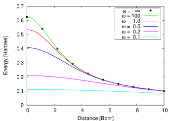
Figure 1: The integral $\gamma^{\text{lr}}_{AB}$ as a function of the inter-atomic distance for different values of the range-separation parameter $\omega$ [bohr^-1]. The decay constants are $\tau_{A}=\tau_{B}=2.0$ bohr^-1. The single dots correspond to the function $\gamma$ given in [2].

As shown in the appendix, this six dimensional integral can be reduced to an efficient one dimensional numerical quadrature:

$$\gamma^{\text{lr}}_{AB}=\frac{2\tau_{A}^{4}\tau_{B}^{4}}{\pi R_{AB}}\int_{0}^{\infty}\frac{\sin(qR_{AB})}{q(q^{2}+\tau_{A}^{2})^{2}(q^{2}+\tau_{B}^{2})^{2}}e^{-q^{2}/4\omega^{2}}\,dq,$$ (42)

where the decay constants $\tau_{A}$ have already been fixed in the treatment of the $\gamma^{\text{fr}}_{AB}$ term. Figure (1) depicts $\gamma^{\text{lr}}_{AB}$ for various values of the range-separation parameter $\omega$. In the limit of $\omega$ going to infinity, the integral needs to reduce to the mentioned original form of $\gamma$ given in [2], because the error function tends to one in this limit. The results show that this is indeed the case.

It should also be mentioned that conventional hybrid functionals involving a fraction of exact exchange may also be realized in the present framework. As an example, Eqs. (33,40,41) with $\omega\to\infty$ give rise to the full Hartree-Fock exchange potential which might be multiplied with an appropriate constant factor. Concurrently, the short range exchange in Eqs. (33,36,4.2) has to be replaced by a conventional full range exchange density functional that is properly weighted.

Concerning the Mulliken approximation which leads to matrix elements in Eqs. (36,40), it should be noted that it completely neglects on-site exchange integrals, which can be restored as describe in Ref. [10]. Here it is worth to point out that within the range-separated formalism, these on-site exchange integrals are expected to much smaller (for $\omega$ small) than in the case of HF or pure hybrid functionals.

5 Total energy and repulsive potential

Considering the results of the previous sections, the total energy of the range-separated DFTB scheme may be summarized as follows:

$$E_{\text{tot}}=\sum_{\mu\nu}\left(H_{\mu\nu}^{\text{(0)}}P_{\mu\nu}+\frac{1}{2}H_{\mu\nu}^{\text{(1)}}\Delta P_{\mu\nu}\right)+E_{\text{rep}},$$ (43)

where we introduced the abbreviation $E_{\text{rep}}$ for an energy contribution that depends solely on the reference density and may hence be precomputed:

$$E_{\text{rep}} = -\frac{1}{2}\sum_{\mu\nu}\left(v^{\text{H}}_{\mu\nu}[\rho_{0}]+v^{\text{xlr}}_{\mu\nu}[\gamma_{0}]\right)P^{0}_{\mu\nu}+E_{\text{NN}}$$ (44)

$$+E_{\text{xsr+c}}[\rho_{0}]-\sum_{\mu\nu}v^{\text{xsr+c}}_{\mu\nu}[\rho_{0}]P^{0}_{\mu\nu}.$$

In the standard DFTB approach the corresponding term is approximated by a sum of short range pair potentials $E_{\text{rep}}=\sum_{AB}V_{AB}(R_{AB})$, which are derived from first principles DFT calculations [48, 2]. A similar approach is possible also in the present context. The additional term in Eq. (44) stemming from the long range exchange is strictly pairwise and decays as the wave function overlap between two centers. From a practical point of view the direct evaluation of $E_{\text{rep}}$ might turn out to be more convenient, since each choice of the range-separation parameter $\omega$ necessitates the construction of new pair potentials.

6 Summary and outlook

In the last sections we derived the theory for a DFTB formalism with range-separated exchange-correlation functionals. It is found that the changes with respect to the original scheme are modest and marginal code modifications are required for the implementation. In order to generate the zero order Hamiltonian and on-site two electron integrals, however, a first principles DFT code featuring range separated functionals needs to be available. Importantly, the computational cost of the scheme grows with respect to the original DFTB, but does not reach the formal scaling of $N^{4}$ for Hartree-Fock based methods. This is due to the integral approximations applied, which allow to evaluate the terms in Eq. (3) with cubic scaling. Hence the diagonalization of the Hamiltonian remains the computational bottleneck.

The presented formalism is also suitable for an straightforward extension of the TD-DFTB [7] approach. The introduction of the long-range term in Eq. 40 will allow to correctly describe charge-transfer excitations [35, 36, 37].

So far we did not discuss the proper choice of the range separation parameter $\omega$. One of the drawbacks of range separated DFT is the system dependence of this parameter: different classes of molecules or even different classes of electronic excitations on the same molecule may require different values of $\omega$ to achieve accurate results [49]. To our knowledge, a criterion for the optimal choice of $\omega$, based on first principles is still lacking. In this regard, the recent work of Baer and coworkers [27] provides an elegant expedient. Here $\omega$ is tuned on a system per system basis to match known conditions for the exact functional (e.g., the ionization potential being equal to the highest occupied orbital energy), escaping the need for an empirical fit to a large training set of molecules. A similar route seems to be promising for the present approximate scheme. In general, the proposed range separated DFTB method could be useful to efficiently scan a large range of parameter values. The optimal value could then be employed in subsequent first principles calculations.

We hope that the presented theory enlarges the applicability of the DFTB method to cases where even local or semi-local first principles DFT approaches face considerable problems The implementation of the formalism is currently under way.

7 Appendix

In section (4.2) the following integral was introduced

$$\gamma^{\text{lr}}_{AB}=\iint F_{A}(\vec{r}_{1})\frac{\text{erf}\left(\omega r_{12}\right)}{r_{12}}F_{B}(\vec{r}_{2})\,d\vec{r}_{1}d\vec{r}_{2},$$ (45)

where

$$F_{A}({\bf r})=\frac{\tau_{A}^{3}}{8\pi}\exp\left(-\tau_{A}|{\bf r}-{\bf R_{A}}|\right),$$ (46)

which we attempt to evaluate in Fourier space. Defining

$$f({\bf q})=\int f({\bf r})e^{i{\bf q}{\bf r}}d{\bf r},$$ (47)

inserting into Eq. (45) twice the identity

$$\delta({\bf r}-{\bf r^{\prime}})=\frac{1}{(2\pi)^{3}}\int e^{i({\bf r}-{\bf r^{\prime}}){\bf k}}d{\bf k},$$ (48)

and integrating out all spatial coordinates, the remaining integrand is easily seen to factorize into a product of Fourier transforms

$$\gamma^{lr}_{AB}=\frac{1}{(2\pi)^{3}}\int F_{A}(-{\bf q})\left(\int\frac{\text{erf}(\omega r)}{r}e^{i{\bf q}{\bf r}}d{\bf r}\right)F_{B}({\bf q})d{\bf q}.$$ (49)

The Fourier transforms of the Slater orbitals $F_{A}$ are known analytically [50]

$$F_{A}({\bf q})=\frac{8\pi\tau_{A}}{(q^{2}+\tau_{A}^{2})^{2}}e^{i{\bf q}{\bf R}_{A}},$$ (50)

and the transform of the long range kernel may be deduced from the transform of the pure $1/r$ kernel given by $4\pi/q^{2}$ and the integral

$$\int_{0}^{\infty}\left[1-\text{erf}(ax)\right]\sin bx=\frac{1}{b}\left(1-e^{-\frac{b^{2}}{4a^{2}}}\right)$$

$$\forall a>0,\,b>0,$$ (51)

given in [51] as formula 6.311. We thus obtain

$$\int\frac{\text{erf}(\omega r)}{r}e^{i{\bf q}{\bf r}}d{\bf r}=\frac{4\pi}{q^{2}}e^{-q^{2}/4\omega^{2}},$$ (52)

and after integration over the angular degrees of freedom in Eq. (49), the end result

$$\gamma^{\text{lr}}_{AB}=\frac{2\tau_{A}^{4}\tau_{B}^{4}}{\pi R_{AB}}\int_{0}^{\infty}\frac{\sin(qR_{AB})}{q(q^{2}+\tau_{A}^{2})^{2}(q^{2}+\tau_{B}^{2})^{2}}e^{-q^{2}/4\omega^{2}}\,dq.$$ (53)

We are especially thankful to Julien Toulouse (UPMC Paris) for fruitful discussions with respect to this study. T.A.N. would like to thank Thomas Frauenheim for continuous support over the last years. Financial aid by the German Science Foundation (DFG, SPP 1243) is also greatly acknowledged.

References

- [1] G. Seifert, H. Eschrig, W. Bieger, Z. Phys. Chem. (Leipzig) 267 (1986) 529.
- [2] M. Elstner, D. Porezag, G. Jungnickel, J. Elsner, M. Haugk, T. Frauenheim, S. Suhai, G. Seifert, Self-consistent-charge density-functional tight-binding method for simulations of complex materials properties, Phys. Rev. B 58 (11) (1998) 7260–7268.
- [3] C. Köhler, G. Seifert, U. Gerstmann, M. Elstner, H. Overhof, T. Frauenheim, Approximate density-functional calculations of spin densities in large molecular systems and complex solids, Phys. Chem. Chem. Phys. 3 (23) (2001) 5109–5114.
- [4] C. Köhler, T. Frauenheim, B. Hourahine, G. Seifert, M. Sternberg, Treatment of collinear and noncollinear electron spin within an approximate density functional based method, J. Phys. Chem. A 111 (26) (2007) 5622–5629.
- [5] M. Elstner, P. Hobza, T. Frauenheim, S. Suhai, E. Kaxiras, Hydrogen bonding and stacking interactions of nucleic acid base pairs: A density-functional-theory based treatment, J. Chem. Phys. 114 (2001) 5149.
- [6] A. Di Carlo, A. Pecchia, L. Latessa, T. Frauenheim, G. Seifert, Introducing Molecular Electronics, Springer, 2005, pp. 153–184.
- [7] T. A. Niehaus, S. Suhai, F. Della Sala, P. Lugli, M. Elstner, G. Seifert, T. Frauenheim, Tight-binding approach to time-dependent density-functional response theory, Phys. Rev. B 63 (8) (2001) 085108.
- [8] T. A. Niehaus, D. Heringer, B. Torralva, T. Frauenheim, Importance of electronic self-consistency in the tddft based treatment of nonadiabatic molecular dynamics, Eur. Phys. J. D 35 (3) (2005) 467–477.
- [9] T. A. Niehaus, Approximate time-dependent density functional theory, J. Mol. Struct.: THEOCHEM 914 (2009) 38.
- [10] T. A. Niehaus, M. Rohlfing, F. Della Sala, A. Di Carlo, T. Frauenheim, Quasiparticle energies for large molecules: A tight-binding-based green’s-function approach, Phys. Rev. A 71 (2) (2005) 022508.
- [11] A. J. Cohen, P. Mori-Sanchez, W. Yang, Insights into current limitations of density functional theory, Science 321 (2008) 792.
- [12] C.-O. Almbladh, U. von Barth, Exact results for the charge and spin densities, exchange-correlation potentials, and density-functional eigenvalues, Phys. Rev. B. 31 (1985) 3231.
- [13] F. Della Sala, A. Görling, Asymptotic behavior of the kohn-sham exchange potential, Phys. Rev. Lett. 89 (2002) 033003.
- [14] J. Chai, M. Head-Gordon, Systematic optimization of long-range corrected hybrid density functionals, J. Chem. Phys. 128 (2008) 084106.
- [15] T. A. Niehaus, A. Di Carlo, T. Frauenheim, Effect of self-consistency and electron correlation on the spatial extension of bipolaronic defects, Organic Electronics 5 (4) (2004) 167–174.
- [16] J. B. Neaton, M. S. Hybertsen, S. G. Louie, Renormalization of molecular electronic levels at metal-molecule interfaces, Phys. Rev. Lett. 97 (21) (2006) 216405.
- [17] E. Fabiano, M. Piacenza, S. D’Agostino, F. Della Sala, Towards an accurate description of the electronic properties of the biphenylthiol/gold interface: The role of exact exchange, J. Chem. Phys. 131 (23) (2009) 234101. doi:10.1063/1.3271393.
- [18] A. Dreuw, M. Head-Gordon, Failure of time-dependent density functional theory for long-range charge-transfer excited states: The zincbacteriochlorin-bacteriochlorin and bacteriochlorophyll-spheroidene complexes, J. Am. Chem. Soc. 126 (12) (2004) 4007–4016.
- [19] M. Wanko, M. Garavelli, F. Bernardi, T. A. Niehaus, T. Frauenheim, M. Elstner, A global investigation of excited state surfaces within time-dependent density-functional response theory, J. Chem. Phys. 120 (4) (2004) 1674–1692.
- [20] C. Toher, A. Filippetti, S. Sanvito, K. Burke, Self-interaction errors in density-functional calculations of electronic transport, Phys. Rev. Lett. 95 (14) (2005) 146402. doi:10.1103/PhysRevLett.95.146402.
- [21] S. H. Ke, H. U. Baranger, W. Yang, Role of the exchange-correlation potential in ab initio electron transport calculations, J. Chem. Phys. 126 (2007) 201102.
- [22] J. A. P. P. M. W. Gill, R. D. Adamson and, Coulomb-attenuated exchange energy density functionals, Mol. Phys 88 (1996) 1005.
- [23] A. Savin, Recent developments and applications of modern density functional theory, Elsevier, 1996, p. 327???357.
- [24] T. Leininger, H. Stoll, H.-J. Werner, A. Savin, Combining long-range configuration interaction with short-range density functionals, Chem. Phys. Lett. 275 (1997) 151.
- [25] T. Yanai, D. P. Tew, N. C. Handy, A new hybrid exchange???correlation functional using the coulomb-attenuating method (cam-b3lyp), Chem. Phys. Lett. 393 (2004) 51.
- [26] H. Iikura, T. Tsuneda, T. Yanai, K. Hirao, A long-range correction scheme for generalized-gradient-approximation exchange functionals, J. Chem. Phys. 115 (2001) 3540.
- [27] R. Baer, E. Livshits, U. Salzner, Tuned range-separated hybrids in density functional theory, Annu. Rev. Phys. Chem. 61 (2010) 85–109.
- [28] A. D. Becke, Density-functional thermochemistry. iii. the role of exact exchange, J. Chem. Phys. 98 (1993) 5648.
- [29] J. Heyd, G. Scuseria, M. Ernzerhof, Hybrid functionals based on a screened coulomb potential, J. Chem. Phys. 118 (2003) 8207.
- [30] J. Heyd, G. Scuseria, M. Ernzerhof, Erratum:“hybrid functionals based on a screened coulomb potential”[j. chem. phys. 118, 8207 (2003)], J. Chem. Phys. 124 (21) (2006) 9906.
- [31] T. Henderson, J. Paier, G. Scuseria, Accurate treatment of solids with the hse screened hybrid, physica status solidi (b) 248 (2010) 767.
- [32] I. Gerber, J. Ángyán, M. Marsman, G. Kresse, Range separated hybrid density functional with long-range hartree-fock exchange applied to solids, The Journal of Chemical Physics 127 (2007) 054101.
- [33] A. Seidl, A. Görling, P. Vogl, J. A. Majewski, M. Levy, Generalized kohn-sham schemes and the band-gap problem, Phys. Rev. B 53 (7) (1996) 3764–3774. doi:10.1103/PhysRevB.53.3764.
- [34] O. Vydrov, G. Scuseria, Assessment of a long-range corrected hybrid functional, The Journal of Chemical Physics 125 (2006) 234109.
- [35] Y. Tawada, T. Tsuneda, S. Yanagisawa, T. Yanai, K. Hirao, A long-range-corrected time-dependent density functional theory, J. Chem. Phys. 120 (2004) 8425.
- [36] T. Stein, L. Kronik, R. Baer, Reliable prediction of charge transfer excitations in molecular complexes using time-dependent density functional theory, Journal of the American Chemical Society 131 (8) (2009) 2818–2820. arXiv:http://pubs.acs.org/doi/pdf/10.1021/ja8087482, doi:10.1021/ja8087482.
- [37] B. M. Wong, M. Piacenza, F. D. Sala, Absorption and fluorescence properties of oligothiophene biomarkers from long-range-corrected time-dependent density functional theory, Phys. Chem. Chem. Phys. 11 (2009) 4498–4508. doi:10.1039/B901743G.
- [38] J. Toulouse, F. m. c. Colonna, A. Savin, Long-range˘short-range separation of the electron-electron interaction in density-functional theory, Phys. Rev. A 70 (2004) 062505. doi:10.1103/PhysRevA.70.062505.
- [39] J. G. Ángyán, I. C. Gerber, A. Savin, J. Toulouse, van der waals forces in density functional theory: Perturbational long-range electron-interaction corrections, Phys. Rev. A 72 (2005) 012510. doi:10.1103/PhysRevA.72.012510.
- [40] J. Toulouse, A. Savin, H. Flad, Short-range exchange-correlation energy of a uniform electron gas with modified electron–electron interaction, Int. J. Quantum Chem. 100 (6) (2004) 1047–1056.
- [41] T. Henderson, B. Janesko, G. Scuseria, Generalized gradient approximation model exchange holes for range-separated hybrids, J. Chem. Phys. 128 (2008) 194105.
- [42] D. Porezag, T. Frauenheim, T. Köhler, G. Seifert, R. Kaschner, Construction of tight-binding-like potentials on the basis of density-functional theory: Application to carbon, Phys. Rev. B 51 (19) (1995) 12947–12957.
- [43] T. Frauenheim, G. Seifert, M. Elstner, T. Niehaus, C. Kohler, M. Amkreutz, M. Sternberg, Z. Hajnal, A. Di Carlo, S. Suhai, Atomistic simulations of complex materials: ground-state and excited-state properties, Journal Of Physics-Condensed Matter 14 (11) (2002) 3015–3047.
- [44] J. C. Slater, G. F. Koster, Simplified lcao method for the periodic potential problem, Phys. Rev. 94 (6) (1954) 1498–1524.
- [45] F. Harris, Analytic evaluation of two-center sto electron repulsion integrals via ellipsoidal expansion, International Journal Of Quantum Chemistry 88 (6) (2002) 701–734.
- [46] J. Budziński, S. Prajsnar, Neumann expansion of the interelectronic distance function for integer powers. i. general formula, The Journal of Chemical Physics 101 (1994) 10783.
- [47] T. A. Niehaus, R. Lopez, J. F. Rico, Efficient evaluation of the fourier transform over products of slater-type orbitals on different centers, J. Phys. A: Math. Theor. 41 (2008) 485205.
- [48] W. Foulkes, R. Haydock, Tight-binding models and density-functional theory, Physical Review B 39 (17) (1989) 12520.
- [49] M. Rohrdanz, J. Herbert, Simultaneous benchmarking of ground-and excited-state properties with long-range-corrected density functional theory, The Journal of Chemical Physics 129 (2008) 034107.
- [50] D. Belkić, H. Taylor, A unified formula for the fourier transform of slater-type orbitals, Phys. Scr. 39 (1989) 226.
- [51] I. Gradsteyn, I. M. Ryzhik, Table of Integrals, Series, and Products, Academic, New York, 1965.