Broadband spectroscopy using two Suzaku observations of the HMXB GX 301$-$2

Abstract

We present the analysis of two Suzaku observations of GX 301$-$2 at two orbital phases after the periastron passage. Variations in the column density of the line-of-sight absorber are observed, consistent with accretion from a clumpy wind. In addition to a CRSF, multiple fluorescence emission lines were detected in both observations. The variations in the pulse profiles and the CRSF throughout the pulse phase have a signature of a magnetic dipole field. Using a simple dipole model we calculated the expected magnetic field values for different pulse phases and were able to extract a set of geometrical angles, loosely constraining the dipole geometry in the neutron star. From the variation of the CRSF width and energy, we found a geometrical solution for the dipole, making the inclination consistent with previously published values.

1. Introduction

The High Mass X-ray Binary (HMXB) system GX 301$-$2 was discovered in 1969 April during a balloon experiment (Lewin et al., 1971; McClintock, Ricker & Lewin, 1971). The system consists of an accreting neutron star (NS) fed by the surrounding stellar wind of the B type emission line companion Wray 977 (Jones, Chetin & Liller, 1974). A recent luminosity estimate derived from atmospheric models puts its distance at $\sim 3$ kpc (Kaper, van der Meer & Najarro, 2006), the value utilized in this paper. The orbital period was established to be $\sim 41$ days (White, Mason & Sanford, 1978) using Ariel 5 observations and was refined with the Burst And Transient Source Experiment (BATSE) to $\sim 41.5$ days with an eccentricity of $\sim 0.46$ (Koh et al., 1997). Doroshenko et al. (2010a) discussed a possible orbital evolution and determined an orbital period of $41.482\pm 0.001$ d, assuming no change in orbital period. Kaper, van der Meer & Najarro (2006) determined that the mass of the companion was in the range $39\,M_{\odot}<M<53\,M_{\odot}$ and the radius of Wray 977 was $\mbox{R}_{*}\sim$62 $\mbox{R}_{\odot}$, obtained by fitting atmosphere models.

The X-ray flux is highly variable throughout an individual binary orbit but follows a distinct pattern when averaged over multiple orbits (see Figure 1). Shortly before the periastron passage, the X-ray luminosity increases drastically in the energy band above $\sim 5$ keV, as seen in Rossi X-ray Timing Explorer (RXTE)/ All Sky Monitor (ASM) data (Leahy, 2002). The NS passes closest to the companion at a distance of $\sim 0.1\mbox{R}_{*}$ (Pravdo et al., 1995). Shortly after the periastron passage, $\phi_{\text{orb}}\sim 0.2$, the X-ray luminosity dips for a short period of time. Leahy (2002) demonstrated that neither a simple spherical wind model nor a circumstellar disk model around Wray 977 are sufficient to describe the observed variations in the folded RXTE/ASM data. An additional stream component is able to account for the sudden increase in X-ray luminosity, as the NS passes trough the stream shortly before periastron and accretes more material. This model also explains a slightly higher X-ray luminosity around $\phi_{\text{orb}}\sim 0.5$, when the NS passes through the accretion stream a second time.

Figure 1.— RXTE/ASM 1.5$-$12 keV light curve folded with the orbital period of 41.48 days. The two lines indicate the times of the orbital phase when the Suzaku observations were performed. The profile shows the strong flux increase during the pre-periastrion flare at orbital phase $\sim 0.9$. For clarity, two binary orbits are shown.

Pulsations with a period of $\sim 700$ s were discovered in the Ariel-5 observations (White et al., 1976), making GX 301$-$2 one of the slowest known pulsars. The pulse period has varied drastically throughout the last $\sim 20$ years (Pravdo & Ghosh, 2001; Evangelista et al., 2010). Prior to 1984, the pulse period stayed relatively constant at 695 s$-$700 s and then spun up between 1985 and 1990 to $\sim 675$ s. From 1993 until the beginning of 2008, the change in the spin reversed again, showing a decline. Fermi/Galactic Burst Monitor (GBM) data have revealed that GX 301$-$2 experienced another spin reversal and briefly spun-up with the pulse period decreasing from $\sim 687$ s to $\sim 681$ s between May 2008 and October 2010. Since October 2010, the pulse period has shown only small variations around $\sim 681$ s.

Most recently, Göğüş, Kreykenbohm & Belloni (2011) discovered a peculiar 1 ks dip in the luminosity of GX 301$-$2, where the pulsations disappeared for one spin cycle during the dip. Several such dips have been previously observed in Vela X-1 (Kreykenbohm et al., 1999, 2008), where it is assumed that the accretion on the NS was interrupted for a short period of time.

The pulse phase average spectrum of GX 301$-$2 is described using a power law with a high energy cutoff. The continuum does not show a strong variation in the intrinsic parameters ($\Gamma,E_{\text{cut}}$, and $E_{\text{fold}}$) throughout the orbit (Mukherjee & Paul, 2004), as seen in two data sets from RXTE, taken in 1996 and 2000, sampling most phases of the binary orbit. One of the major characteristics of the X-ray spectrum of GX 301$-$2 is the high and strongly variable column density of its line-of-sight absorber throughout the orbit, indicative of a clumpy stellar wind ($N_{\text{H}}=10^{22}-10^{24}$ cm^-2). In addition to the high column density, a very bright Fe K$\alpha$ emission line can be observed. This line has shown a strong correlation with the observed luminosity, indicating that the line is produced by local clumpy matter surrounding the neutron star (Mukherjee & Paul, 2004). Kreykenbohm et al. (2004) used the RXTE data set from 2000 to perform phase resolved spectroscopy and showed that an absorbed and partially covered pulsar continuum (power law with Fermi-Dirac cutoff) as well as a reflected and absorbed pulsar continuum were consistent with the data.

A cyclotron resonance scattering feature (CRSF) at $\sim 35$ keV was first discovered with Ginga (Mihara, 1995). Orlandini et al. (2000) found systematic deviations from a power law continuum at $\sim 20$ and $\sim 40$ keV in BeppoSAX, where the former could not be confirmed as a CRSF due to the proximity of the continuum cutoff. Kreykenbohm et al. (2004) excluded the existence of a CRSF at $\sim 20$ keV and showed that the CRSF centroid energy varies between 30–38 keV over the pulse rotation of the NS. Furthermore, they showed that the CRSF centroid energy and width are correlated.

We report on two observations of GX 301$-$2 performed with the Suzaku satellite in mid 2008 and early 2009. This paper is structured as follows: Section 2 discusses the observations and data reduction. Section 3 shows the phase averaged results. Section 4 discusses the pulse profiles and phase resolved spectra. Sections 5 and 6 discuss the results and conclusions, respectively.

2. Observation and Data Reduction

Suzaku observed GX 301$-$2 on 2008 August 25 with an exposure time of $\sim 10$ ks (ObsID 403044010; hereafter Obs. 1). The observation was cut short by a set of target of opportunity observations and was continued on 2009 January 5, acquiring an additional $\sim 60$ ks exposure time (ObsID 403044020; Obs. 2). Both main instruments, the X-ray Imaging Spectrometer (XIS; Mitsuda et al., 2007) and the Hard X-ray Detector (HXD; Takahashi et al., 2007) were used in these observations. The two observations correspond to orbital phases of 0.19 (Obs. 1) and 0.38 (Obs. 2), where Obs. 1 falls into the lowest flux part of the binary orbit (see Figure 1). The $2-10$ keV absorbed flux was $1.6\times 10^{-10}$ erg cm^-2 s^-1 for Obs. 1 and $\sim 8\times 10^{-10}$ erg cm^-2 s^-1 for Obs. 2 (see Table 1 for details). Both observations were performed using the HXD nominal pointing to enhance the sensitivity of the HXD detectors.

The XIS detectors consist of two front illuminated (FI) CCDs XIS 0 and 3, and one back illuminated (BI) CCD, XIS 1. All three instruments are sensitive between $\sim 0.5$ keV and $\sim 11$ keV, although the two FI cameras have a higher sensitivity above $\sim 2$ keV, and the BI chip is more sensitive below $\sim 2$ keV. To minimize possible pile-up, the XIS instruments were operated with the 1/4 window option with a readout time of 2 s. Data were taken in both $3\times 3$ and $5\times 5$ editing modes, which were extracted individually with the Suzaku FTOOLS version 16 as part of HEASOFT 6.9. The unfiltered XIS data were reprocessed with the most recent calibration files available and then screened with the standard selection criteria as described by the Suzaku ABC guide. The response matrices (RMFs) and effective areas (ARFs) were weighted according to the exposure times of the different editing modes. The XIS data were then grouped with the number of channels per energy bin corresponding to the half width half maximum of the spectral resolution, i.e. grouped by 8, 12, 14, 16, 18, 20, and 22 channels starting at 0.5, 1, 2, 3, 4, 5, 6, and 7 keV, respectively (M. A. Nowak, 2010, private communication). The XIS spectral data were used in the energy range of $2-10$ keV for reasons described below.

The HXD consists of two non-imaging instruments: the PIN silicon diodes (sensitive between 12–60 keV) and the GSO/BGO phoswich counters (sensitive above $\sim 30$ keV). To determine the PIN background, the Suzaku HXD team provides the tuned PIN Non X-ray Background (NXB) for each individual observation. In addition, the cosmic X-ray Background (CXB) was simulated following the example in the ABC guide and both backgrounds were added together. The PIN data were grouped by a factor of 5 below and by a factor of 10 above 50 keV for Obs. 1. In Obs. 2 the channels were grouped by 3 throughout the whole energy range. GSO data were extracted and binned following the Suzaku ABC guide. The PIN data energy range of 15–60 keV and the GSO data energy range of $50-90$ keV were used for the phase averaged analysis. Due to the short exposure times, no GSO data were extracted in Obs. 1 and in the phase resolved analysis of Obs. 2.

2.1. XIS Responses

GX 301$-$2 is a source with very large and highly variable photoelectric absorption in the line of sight as well as a very strong Fe K$\alpha$ emission line. For spectral modeling, the calculated responses of the XIS detectors showed a ‘leakage’ emission level (Matsumoto et al., 2006), which stemmed from the instrument characteristics. That is, a small fraction of an event charge cloud is registered at energies below the peak energy, creating a ’low energy tail’ in the spectrum. This ‘tail’ is about three orders of magnitude weaker than the intensity of the peak count rate of the measured photon. The response to the Fe line is therefore described as a Gaussian plus a constant at lower energies, approximately three orders of magnitude below the peak value and extending to below 1 keV. Due to the strong Fe K$\alpha$ line and the very strong absorption in this source, the constant level response of the Fe line extends above the measured flux below 2 keV. This results in significant residuals below $\sim 2$ keV, which seem to be stronger for the BI spectrum then for that of the FI CCD. Figure 2 shows the phase averaged spectrum from the second observation of GX 301$-$2 and the best fit models using the HEASOFT generated XIS responses as detailed in section 3.

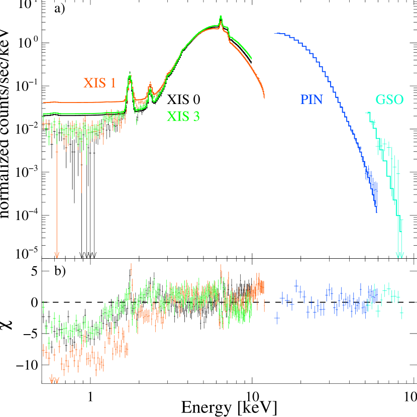
Figure 2.— (a) Best fit models of the Suzaku GX 301$-$2 second observation for the 3 individual XIS instruments, and the two HXD instruments. At lower energies, one clearly sees the constant level in the modeled flux discussed in the text. (b) shows that the residuals below $\sim 2$ keV are very pronounced.

Together with the Suzaku Guest Observer Facility (GOF), which provided for us an experimental response parameter file where the ‘low energy tail’ is ignored, we studied this behavior in more detail. This new response for all three instruments was applied to the individual XIS spectra. Due to the fact that the new response completely excluded the missing ‘tail’, we now observed an excess of the data with respect to the model below $\sim 2\,$keV. The introduction of additional power law and/or black body components could improve the fits at lower energies. Due to the fact that the true level of the tail is not known, these additional components cannot be interpreted physically, and we decided to use the original response matrix and confine the selected XIS energy range to above 2 keV.

3. Phase averaged spectrum

3.1. Spectral modeling

Phase averaged broad band spectra in the 2–60 keV (Obs. 1) and 2–90 keV (Obs. 2) energy ranges were obtained. From the technical description of the XIS instruments, it is known that small discrepancies, e.g., in fitted power law slope, have been observed between FI and BI XIS instruments. A difference of $\sim 0.05$ in the power law index has been observed in calibration data and was also observed here. When modeling the FI and BI instruments with a common power law index, the residuals of the BI instrument show a systematic deviation. However, only the FI or BI instruments could be modeled together with the HXD instruments. Due to this fact and the higher sensitivity of the FI XIS instruments above 2 keV, we concentrated our discussion on the results obtained with the two FI instruments. Each data set, FI and BI, was modeled individually with the HXD data to compare the differences in the continuum. We found that when using the FI and BI instruments individually with the HXD instruments, in both observations the best fit spectral values are consistent with each other within error bars, indicating that the usage of the HXD reduced the observed discrepancies in the power law parameters.

The continuum model for pulsars can so far only be modeled with empirical models, consisting of a powerlaw with a cutoff at higher energies, which is typical for this kind of source (Coburn, 2001). Three empirical models are widely used: the simple high energy cutoff (highecut) and the Fermi-Dirac cutoff (fdcut, Tanaka, 1986) both are used in combination with a simple power law component. In addition, the negative-positive exponential powerlaw model NPEX (Mihara, 1995) is a slightly more complicated model including the power law component. For the data analyzed in this work, the best results have been obtained with the fdcut model:

$$I_{\text{cont}}=A_{\text{PL}}\frac{E^{-\Gamma}}{\text{exp}(E-E_{\text{cut}}/E_{\text{fold}})+1},$$ (1)

where $A_{\text{PL}}$ is the normalization at 1 keV, $E_{\text{cut}}$ is the cutoff energy, and $E_{\text{fold}}$ is the folding energy of the Fermi-Dirac cutoff. For the Obs. 1 and Obs. 2 FI data sets the best fit $\chi^{2}$’s were 260 and 542 with 245 and 267 degrees of freedom (dof), respectively (see Figure 3 and 4). Replacing the smoother Fermi-Dirac cutoff with the highecut model in Obs. 2,resulted in slightly worse residuals ($\Delta\chi^{2}\approx 15$) compared to the best fit results of the FD-cutoff model (Figure 3 d) and an emission line-like residual at $\sim 35$ keV, which is most likely due to the sharp break of the power law at the cutoff energy in this model. In comparison, the NPEX model shows even worse residuals ($\Delta\chi^{2}\approx 200$) and only results in reasonable fits when the exponential curvature at higher energies is independent in the partially and fully covered component.

The best fit cutoff energy is very close to that of the observed CRSF feature (see below) and these two parameters are rather strongly correlated (see Figure 5). To avoid a degeneracy of the CRSF values due to a changing cutoff energy, $E_{\text{cut}}$ was frozen in all the fits to the best fit value from the Obs. 2 FI spectrum (29.2 keV).

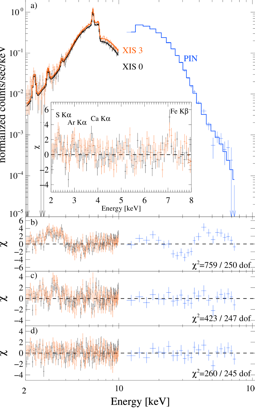
Figure 3.— Data and best fit model for Obs. 1. a) shows the data and the best fit model. The inset shows the residual for the different emission lines observed in XIS data, where the Fe K$\alpha$ line is already included in the model. b) shows the best fit residuals without partial covering and the CRSF. c) has only the CRSF added, and d) has both componenst included.

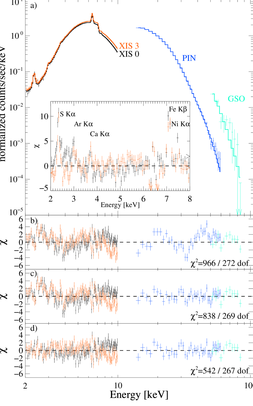
Figure 4.— Same as Figure 3 for Obs. 2. In this case b) shows the residuals without partial covering and the CRSF, c) has only the CRSF added and d) has both components included.

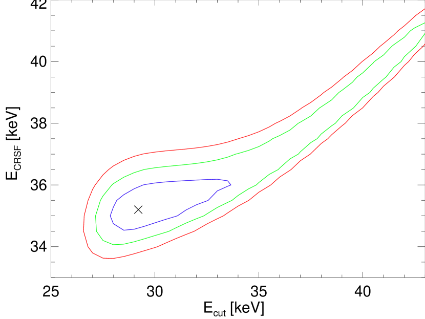
Figure 5.— Contour plots of $E_{\text{CRSF}}$ vs $E_{\text{cut}}$. The different contours indicate the 1, 2, and 3 sigma contours for the FI spectrum of Obs. 2. The X indicates the best fit values for both parameters: $E_{\text{cut}}=29.2$ keV and $E_{\text{CRSF}}=35.2$ keV.

Previous observations of GX 301$-$2 indicated the existence of clumps in the stellar wind (Kreykenbohm et al., 2004; Mukherjee & Paul, 2004), which were modeled using partial covering absorption in addition to fully covered photoelectric absorption of the smooth stellar wind. In the present analysis, the low energy portion of the spectrum also required a partial covering component (Figure 3b and 4b), which was modeled using the TBnew model (Wilms et al., 2011, in prep.), an updated version of the existing TBabs model (Wilms, Allen & McCray, 2000). In addition, a non-relativistic, optically-thin Compton scattering component cabs was included, as is necessary for column densities $N_{\text{H}}>5\times 10^{22}$ cm^-2, where the plasma becomes Compton thick and part of the emission is scattered out of the line of sight. The $N_{\text{H}}$ values from TBabs and from the cabs component were set equal and treated as one model component for the smooth stellar wind ($N_{\text{H,1}}$ = TBabs1*cabs1) and a second component for the clumpy partial coverer ($N_{\text{H,2}}$ = TBabs2*cabs2). The $N_{\text{H,1}}$ and $N_{\text{H,2}}$ column densities were left independent of each other. For spectral fitting the abundances of Wilms, Allen & McCray (2000) and the cross-sections (Verner et al., 1996) were used in all data sets.

Both observations show residuals to the continuum in the $35-40$ keV energy range, which we interpret as the previously observed CRSF (Mihara, 1995; Kreykenbohm et al., 2004). Modeling these residuals with an absorption line with a Gaussian optical depth (gabs) improved the residuals significantly in both observations (see Figures 3 and 4). The best fit values of $E_{\text{CRSF}}=42.5^{+3.2}_{-6.0}$ keV and $35.2^{+1.4}_{-0.9}$ keV for Obs. 1 and Obs. 2, respectively, are consistent within 90% confidence intervals. The widths of the CRSFs, $\sigma_{\text{CRSF}}=9.5^{+1.6}_{-2.8}$ keV (Obs. 1) and $7.8^{+1.1}_{-0.9}$ keV (Obs. 2), are also consistent within errors. An increase of $\sigma_{\text{CRSF}}$ with higher centroid energy, as previously observed in RXTE data (Kreykenbohm et al., 2004), could not be detected, although the best fit values hint at such a behavior. Table 1 shows the best fit values for the continuum with a gabs CRSF line where the given errors are 90% confidence values. To calculate the significance of the CRSF in the first and weaker observation, the null hypothesis approach was applied, where 10,000 spectra were created with Monte Carlo simulations using the best fit parameters without the CRSF. Gaussian uncertainties were used for the individual model parameter. Each model was fitted with and without the CRSF line to compare how much an inclusion of the line actually improves the fit. In $\sim 99.6\%$ of all fits, no CRSF feature were observed with a larger optical depth than the observed lower limits of $\tau=10.3$, making the existence of the feature significant with $\sigma\sim 3$. Including the CRSF in the real data, the best fit improved by a $\Delta\chi^{2}=100$. A similar improvement of $\chi^{2}$ was only observed in $\sim 0.1\%$ ($\sigma\sim 3.3$) of the simulated spectra, concluding that the observed line in the first observation is indeed real. For the second observation, the line was even more pronounced, where the exclusion of the CRSF increased the $\chi^{2}$ by $\sim 200$.

Table 1Phase averaged spectral parameters with the GABS model component for best fit spectrum

Parameter	403044010 (10ks)		403044020 (60ks)
	FI	BI	FI	BI
$N_{\text{H,1}}[10^{22}$ cm-2]	$16.6^{+3.5}_{-3.3}$	16.6 (frozen)	$20.9^{+3.5}_{-3.3}$	20.9 (frozen)
Abund Ca	1.55 (frozen)	1.55 (frozen)	$1.55^{+0.39}_{-0.18}$	$1.98^{+0.41}_{-0.49}$
Abund Fe	1.17 (frozen)	1.17 (frozen)	$1.17^{+0.04}_{-0.03}$	$1.04^{+0.03}_{-0.04}$
$N_{\text{H,2}}[10^{22}$ cm-2]	$76.9^{+3.9}_{-3.1}$	76.9 (frozen)	$28.4^{+1.0}_{-1.0}$	28.4 (frozen)
$\Gamma$	$0.83^{+0.08}_{-0.06}$	$0.82^{+0.09}_{-0.08}$	$0.96^{+0.06}_{-0.04}$	$0.98^{+0.03}_{-0.03}$
$A_{\text{PL,1}}$ $[10^{-3}]^{1}$ fully covered	$1.68^{+0.67}_{-0.50}$	$1.38^{+0.20}_{-0.20}$	$1.1^{+1.1}_{-0.5}$	$4.70^{+0.91}_{-0.79}$
$A_{\text{PL,2}}$ $[10^{-3}]^{1}$ part. covered	$92.5^{+16.1}_{-10.0}$	$90.0^{+16.2}_{-8.1}$	$215.5^{+25.1}_{-8.9}$	$266.4^{+17.9}_{-15.5}$
$E_{\text{cut}}$ [keV]	29.2 (frozen)	29.2 (frozen)	$29.2^{+13.5}_{-2.1}$	29.2 (frozen)
$E_{\text{fold}}$ [keV]	$10.3^{+3.1}_{-3.0}$	$8.3^{+2.0}_{-1.4}$	$5.7^{+0.4}_{-2.5}$	$5.6^{+0.2}_{-0.2}$
$E_{\text{CRSF}}$ [keV]	$42.5^{+3.2}_{-6.0}$	$39.7^{+3.7}_{-3.9}$	$35.2^{+1.4}_{-0.9}$	$34.9^{+0.9}_{-0.5}$
$\sigma_{\text{CRSF}}$ [keV]	$9.5^{+1.6}_{-2.8}$	$8.6^{+2.0}_{-2.1}$	$7.8^{+1.1}_{-0.9}$	$7.4^{+0.5}_{-0.5}$
$\tau_{\text{CRSF}}$	$29.3^{+17.7}_{-19.0}$	$18.9^{+14.8}_{-9.7}$	$12.0^{+37.7}_{-4.5}$	$10.6^{+1.8}_{-1.4}$
$E_{\text{S~{}K}\alpha}$ [keV]	$2.33^{+0.01}_{-0.02}$	$2.31^{+0.03}_{-0.03}$	$2.33^{+0.01}_{-0.01}$	$2.34^{+0.01}_{-0.01}$
$I_{\text{S~{}K}\alpha}[10^{-5}]^{2}$	$2.34^{+0.61}_{-0.64}$	$2.44^{+0.96}_{-0.89}$	$5.36^{+0.50}_{-0.50}$	$4.24^{+0.68}_{-0.67}$
EQW${}_{\text{S~{}K}\alpha}^{3}$ [eV]	$860^{+1534}_{-585}$	$1109^{+1313}_{-947}$	$671^{+491}_{-172}$	$965^{+612}_{-445}$
$E_{\text{Ar~{}K}\alpha}$ [keV]	$2.96^{+0.03}_{-0.03}$	$3.02^{+0.06}_{-0.05}$	$3.00^{+0.01}_{-0.02}$	$3.04^{+0.02}_{-0.02}$
$I_{\text{Ar~{}K}\alpha}[10^{-5}]^{2}$	$1.72^{+0.62}_{-0.69}$	$1.00^{+0.94}_{-0.48}$	$2.74^{+0.55}_{-0.54}$	$4.53^{+0.94}_{-0.88}$
EQW${}_{\text{Ar~{}K}\alpha}^{3}$ [eV]	$179^{+502}_{-164}$	$110^{+308}_{-110}$	$38^{+29}_{-21}$	$64^{+38}_{-37}$
$E_{\text{Ca~{}K}\alpha}$ [keV]	$3.73^{+0.05}_{-0.04}$	$3.76^{+0.07}_{-0.06}$	$3.70^{+0.02}_{-0.01}$	$3.71^{+0.03}_{-0.03}$
$I_{\text{Ca~{}K}\alpha}[10^{-5}]^{2}$	$1.71^{+0.77}_{-0.83}$	$2.45^{+1.33}_{-1.35}$	$4.72^{+0.95}_{-0.99}$	$4.95^{+1.68}_{-1.71}$
EQW${}_{\text{Ca~{}K}\alpha}^{3}$ [eV]	$69^{+140}_{-69}$	$100^{+154}_{-100}$	$14^{+10}_{-8}$	$14^{+14}_{-14}$
$E_{\text{Fe~{}K}\alpha}$ [keV]	$6.399^{+0.007}_{-0.006}$	$6.410^{+0.010}_{-0.010}$	$6.409^{+0.003}_{-0.001}$	$6.424^{+0.003}_{-0.002}$
$\sigma_{\text{Fe~{}K}\alpha}$ [eV]	$13^{+22}_{-2}$	$<31$	$<5$	$<7$
$I_{\text{Fe~{}K}\alpha}[10^{-4}]^{2}$	$7.16^{+0.36}_{-0.22}$	$6.96^{+0.63}_{-0.63}$	$19.20^{+0.29}_{-0.30}$	$22.9^{+0.61}_{-0.58}$
EQW${}_{\text{Fe~{}K}\alpha}^{3}$ [eV]	$241^{+53}_{-35}$	$230^{+58}_{-52}$	$133^{+27}_{-4}$	$142^{+10}_{-10}$
$E_{\text{Fe~{}K}\beta}$ [keV]	$7.06^{+0.03}_{-0.03}$	$7.04^{+0.04}_{-0.04}$	$7.09^{+0.01}_{-0.01}$	$7.09^{+0.02}_{-0.02}$
$I_{\text{Fe~{}K}\beta}[10^{-4}]^{2}$	$1.19^{+0.29}_{-0.35}$	$1.54^{+0.59}_{-0.60}$	$2.65^{+0.27}_{-0.25}$	$4.50^{+0.53}_{-0.56}$
EQW${}_{\text{Fe~{}K}\beta}^{3}$ [eV]	$43^{+33}_{-29}$	$56^{+53}_{-51}$	$21^{+7}_{-5}$	$32^{+9}_{-10}$
$E_{\text{Ni~{}K}\alpha}$ [keV]	$-$	$-$	$7.46^{+0.02}_{-0.02}$	$7.51^{+0.11}_{-0.06}$
$I_{\text{Ni~{}K}\alpha}[10^{-4}]^{2}$	$-$	$-$	$1.57^{+0.25}_{-0.25}$	$0.67^{+0.62}_{-0.62}$
EQW${}_{\text{Ni~{}K}\alpha}^{3}$ [eV]	$-$	$-$	$15^{+9}_{-7}$	$5.7^{+13.4}_{-5.7}$
Flux${}_{2-10\,\text{keV}}^{4}$ absorb.	$1.61^{+0.04}_{-0.15}$	$1.63^{+0.03}_{-0.07}$	$7.98^{+0.00}_{-1.42}$	$9.04^{+0.04}_{-0.06}$
Flux${}_{2-10\,\text{keV}}^{4}$ unabsorb.	$16.3^{+2.0}_{-1.1}$	$16.0^{+0.8}_{-0.7}$	$31.8^{+1.3}_{-0.2}$	$35.9^{+1.0}_{-0.4}$
$C_{\text{XIS3}}/C_{\text{PIN}}/C_{\text{GSO}}^{5}$	$0.93^{+0.02}_{-0.02}/1.18^{+0.04}_{-0.04}$ / –	–/ $1.12^{+0.07}_{-0.06}$ / –	$0.951^{+0.003}_{-0.003}/1.31^{+0.02}_{-0.02}/1.39^{+0.12}_{-0.12}$	– / $1.17^{+0.02}_{-0.02}/1.27^{+0.11}_{-0.11}$
$\chi^{2}$/dof	260 / 245	145 / 130	542 / 267	328 / 150
(1)Units are ph keV-1 cm-2 s-1, (2) Units are ph cm-2 s-1, (3) Values of EQWs are determined relative to the abs. continuum,
(4) Absorbed and unabsorbed flux units are $[10^{-10}$ erg sec-1 cm${}^{-2}]$, (5) Values of $C$ are with respect to XIS 0 for the FI fits and XIS 1 for the BI fits.

The CRSF can alternatively be described with the Lorenzian shaped cyclabs XSPEC model (Mihara et al., 1990). Cyclabs is described by the centroid energy $E_{\text{CRSF}}$, the width $\sigma_{\text{CRSF}}$, and the resonance depth $\tau_{\text{CRSF}}$, similar to the gabs parameters. The best fit continuum parameters are consistent with the best fit values determined with the gabs component. The cutoff energy with a best fit value of $E_{\text{cut}}=31.2^{+5.1}_{-2.9}$ keV is consistent with the value obtained with the gabs model. The observed centroid energies of $E_{\text{CRSF}}=35.0^{+3.0}_{-2.3}$ keV and $31.6^{+1.0}_{-0.5}$ keV are of the order of $10-20\%$ lower than the energies obtained with the gabs model. This discrepancy stems from a different calculation of the line centroid energy and is described in detail in Nakajima, Mihara & Makishima (2010). The width $\sigma_{\text{CRSF}}=11.2^{+3.8}_{-3.0}$ keV and $12.3^{+1.7}_{-1.3}$ keV for Obs. 1 and Obs. 2, respectively, is bigger than with the gabs model. The $\chi^{2}$ / dof values of 260 / 245 and 548 / 267 for the two observations using the cyclabs model and thus were not a better fit when compared to the gabs model. For the final discussion we use the values determined by the gabs model.

Several emission features were observed in the residuals of the fits in both observations and were subsequentially modeled with Gaussian emission lines (see Figures 3 and 4, inlay). The width of each line was set equal to that of the Fe K$\alpha$ emission line, while the intensities were left to vary independently. Energies were loosely constrained around the expected values of neutral material to avoid runaway of the line energies.

A constant (const) was applied, taking small instrumental differences in the overall flux normalization into account. The constant was fixed at 1 for XIS 0 and was left free for the other instruments. $C_{\text{XIS3}}$, $C_{\text{PIN}}$ and $C_{\text{GSO}}$ in Table 1 are the cross calibration constants with respect to XIS 0 for FI fits and with respect to XIS 1 for the BI fits.

The final model had the form: const*$N_{\text{H,1}}$ (PL1+ $N_{\text{H,2}}$*PL2)* fdcut*gabs+ $6\times$Gaussians, where the power law indices of PL1 and PL2 are set to be equal to each other. The individual power law normalizations were independent and were used to calculate the fraction of the partial covering.

Table 1 summarizes the best fit values for both observations and for the individual FI / BI data sets. For the interpretation we will concentrate on the FI data for both observations, for reasons mentioned above.

3.2. Spectral results

The best fit spectral parameters were generally consistent with previous observations, with the exception of the cutoff energy. With a value of $29.2^{+13.5}_{-2.1}$ keV, $E_{\text{cut}}$ was significantly higher than the $\sim 20$ keV value measured in previous RXTE (Mukherjee & Paul, 2004) and BeppoSAX (La Barbera et al., 2005) observations, although these observations used slightly different spectral models for the cutoff energy. Kreykenbohm et al. (2004) used also the here applied Fermi–Dirac cutoff, resulting in cutoff energies of $10-15$ keV. The folding energy for Obs. 1, $E_{\text{fold}}=10.3^{+3.1}_{-3.0}$ keV, is consistent with values obtained for a similar orbital phase with BeppoSAX (La Barbera et al., 2005). In Obs. 2, the value of $E_{\text{fold}}=5.7^{+0.4}_{-2.5}$ keV is consistent with the RXTE data for the pre-periastron flare and the periastron passage (Kreykenbohm et al., 2004).

The observed column densities for the absorption due to the smooth stellar wind ($N_{\text{H,1}}$) were consistent between both observations. A larger difference could be observed in the column density associated with the absorption due to the clumped wind ($N_{\text{H,2}}$), where the best fit value of Obs. 1 is almost a factor three larger than that of Obs. 2. In addition to the H column density in the TBnew model, the relative Ca and Fe abundances were also left independent in Obs. 2. The best fit values are measured from the Ca and Fe K edges at $4.1$ keV and $7.1$ keV, respectively, and were slightly higher than solar abundances: $1.55^{+0.39}_{-0.18}$ for Ca and $1.17^{+0.04}_{-0.03}$ for Fe. For the first observation, the Ca and Fe abundances could not be well constrained and were fixed to 1.55 for Ca and 1.17 for Fe.

The partial covering fractions can be calculated from the measured normalization values of the two power law components, $A_{\text{PL1}}$ and $A_{\text{PL2}}$:

$$\text{Cvr. Frac.}=\frac{A_{\text{PL2}}}{A_{\text{PL1}}+A_{\text{PL2}}}.$$ (2)

The factor is almost unity in both observations due to the dominance of the $A_{\text{PL2}}$ value. Similar large covering fractions have been observed in XMM-Newton data (Fürst et al., 2011b) and in the RXTE data (Mukherjee & Paul, 2004), indicating that the covering fraction does not change significantly for different parts of the orbit. The spectrum softened slightly from $\Gamma=0.83^{+0.08}_{-0.06}$ for Obs. 1 to $0.96^{+0.06}_{-0.04}$ for Obs. 2.

The Fe K$\alpha$ line was detected at $6.409^{+0.003}_{-0.001}$ keV (Obs. 2), which is, given the instrumental gain systematics, consistent with neutral Fe. In addition, the following lines have also been observed in both observations: S K$\alpha$ line, Ar K$\alpha$ line, Ca K$\alpha$ line, Fe K$\beta$ line, and the Ni K$\alpha$ line, all with energies consistent with neutral material (e.g. Kaastra & Mewe, 1993). Note that the Ni K$\alpha$ line was not detected in the fainter first observation. The observed line intensities are summarized in table 1 with 90% confidence errors. The values are consistent between the FI and BI instruments. The widths of the lines were set to be equal to the Fe K$\alpha$ width within each observation, which was found to be $13^{+22}_{-2}$ eV for Obs. 1 and had an upper limit of 5 eV in Obs. 2 (FI values). The Compton shoulder to the Fe K$\alpha$ line, as observed by the Chandra observatory (Watanabe et al., 2003), was not significantly detected in either observation. The observation of Watanabe et al. (2003) was performed in the pre-periastron phase, where the luminosity was higher than in the two Suzaku observations. A Compton shoulder has also been observed with XMM-Newton in data taken during another pre-periastron flare (Fürst et al., 2011b).

4. Phase resolved analysis

Barycentric and binary corrected light curves for different energy bands were extracted for both observations using the orbital parameters from Koh et al. (1997) with an updated orbital period and periastron time $t_{0}$ determined by Doroshenko et al. (2010a). Due to the strong variability of the pulse period on short time scales, individually determined pulse periods were used for each observation. An accurate pulse period could be established for Obs. 2, but not for Obs. 1 due to its short duration of 10 ks. For the second observation the calculated pulse period had a value of $P=685.4\pm 0.9$ s. The Fermi/GBM instrument measures the pulse period of GX 301$-$2 on a regular basis, resulting in values of $P=687.28$ s for Obs. 1 and $P=685.75$ s for Obs. 2 (Finger, 2011, priv. comm). To create the pulse profiles, the Fermi/GBM-provided pulse periods and epoch times for each observation were used.

We studied the energy dependent pulse profiles for Obs. 1 and Obs. 2. Both pulse profiles are very similar, showing a double peak shape where the main peak (P1) is broader below 10 keV. The second peak (P2) stays rather constant in width, but increases its relative intensity toward higher energies. As an example, the pulse profile for Obs. 2 in different energy bands is shown in Figure 6. Comparing these pulse profiles with previous RXTE and BeppoSAX data showed that the general shape is consistent through all parts of the orbit.

Figure 6.— Pulse profiles for different energy bands for Obs. 2. The two peaks are indicated in the top panel. The bottom pannel shows the selection of phase bins which were used for phase resolved spectroscopy.

The data of the longer Obs. 2 were divided into 10 equally spaced phase bins and individual spectra were extracted for the XIS and PIN instruments. Figure 6 shows the individual phase bins in the lowest panel. This division resulted in an exposure time in each phase bin of $\sim 5-6$ ks for each individual instrument. No GSO data were used in this analysis due to the reduced exposure time per phase bin. For spectral analysis, the phase averaged model was applied to all phase bins, resulting in best fit values summarized in Table 2, as well as Figure 7. Again the cutoff energy was frozen to the phase averaged value of 29.2 keV to avoid the previously discussed degeneracy with $E_{\text{CRSF}}$.

Table 2Phase resolved spectral parameter from Obs. 2 for FI data. Same model as phase averaged data.

Parameter	PB1	PB2	PB3	PB4	PB5	PB6	PB7	PB8	PB9	PB10
$N_{\text{H,1}}[10^{22}$/cm2]	$19.2_{-7.7}^{+10.2}$	$20.0_{-6.4}^{+7.9}$	$36.1_{-7.4}^{+4.6}$	$20.2_{-20.2}^{+23.6}$	$32.4_{-11.3}^{+8.3}$	$22.8_{-7.3}^{+7.9}$	$25.3_{-4.7}^{+4.4}$	$12.2_{-4.6}^{+6.5}$	$21.4_{-7.3}^{+7.9}$	$24.6_{-5.5}^{+5.4}$
$N_{\text{H,2}}[10^{22}$/cm2]	$32.6_{-1.9}^{+5.0}$	$30.9_{-5.4}^{+4.9}$	$21.3_{-4.5}^{+13.8}$	$25.0_{-20.6}^{+21.0}$	$18.7_{-3.6}^{+9.3}$	$26.7_{-4.1}^{+5.0}$	$32.7_{-2.8}^{+4.1}$	$35.2_{-2.8}^{+4.0}$	$29.5_{-3.9}^{+3.9}$	$31.6_{-2.8}^{+2.6}$
$\Gamma$	$1.22_{-0.11}^{+0.08}$	$1.30_{-0.04}^{+0.04}$	$0.93_{-0.04}^{+0.04}$	$0.91_{-0.04}^{+0.03}$	$1.20_{-0.04}^{+0.04}$	$1.07_{-0.22}^{+0.10}$	$0.74_{-0.05}^{+0.05}$	$0.56_{-0.04}^{+0.04}$	$0.67_{-0.05}^{+0.05}$	$1.15_{-0.06}^{+0.06}$
$A_{\text{PL,1}}[10^{-2}]^{1}$ ful. cov.	$0.97_{-0.70}^{+3.28}$	$1.35_{-0.90}^{+3.13}$	$10.12_{-7.27}^{+8.47}$	$0.29_{-0.28}^{+25.73}$	$8.69_{-7.55}^{+24.37}$	$1.92_{-1.44}^{+4.56}$	$2.03_{-1.00}^{+1.53}$	$0.16_{-0.27}^{+0.09}$	$0.83_{-0.57}^{+1.74}$	$2.36_{-1.33}^{+2.62}$
$A_{\text{PL,2}}[10^{-2}]^{1}$ par. cov.	$24.4_{-3.4}^{+4.1}$	$44.8_{-4.3}^{+4.9}$	$17.4_{-8.0}^{+6.6}$	$27.4_{-25.9}^{+2.2}$	$41.1_{-22.5}^{+77.1}$	$27.7_{-4.3}^{+3.9}$	$10.8_{-2.0}^{+2.0}$	$10.6_{-1.0}^{+1.0}$	$11.3_{1.4}^{+1.4}$	$19.3_{-2.7}^{+3.0}$
$E_{\text{fold}}$ [keV]	$7.4_{-2.3}^{+14.1}$	$6.13_{-0.35}^{+0.38}$	$5.6_{-0.3}^{+0.4}$	$5.5_{-0.4}^{+0.5}$	$5.9_{-0.6}^{+0.7}$	$4.1_{-0.9}^{+5.0}$	$4.5_{-0.6}^{+0.8}$	$5.0_{-0.4}^{+0.5}$	$4.4_{-0.3}^{+0.3}$	$5.0_{-0.3}^{+0.4}$
$E_{\text{CRSF}}$ [keV]	$38.7_{-5.7}^{+9.3}$	$29.8_{-1.2}^{+1.6}$	$32.1_{-1.4}^{+1.9}$	$34.6_{-2.3}^{+3.1}$	$38.0_{-2.4}^{+2.8}$	$38.3_{-8.2}^{+22.9}$	$35.4_{-3.0}^{+4.1}$	$35.7_{-1.5}^{+1.9}$	$31.1_{-1.0}^{+1.4}$	$27.5_{-0.8}^{+1.1}$
$\sigma_{\text{CRSF}}$ [keV]	$10.3_{-2.1}^{+3.7}$	$5.1_{-1.1}^{+1.7}$	$6.4_{-0.9}^{+1.2}$	$7.3_{-1.1}^{+1.4}$	$6.3_{-1.1}^{+1.3}$	$15.1_{-6.0}^{+15.0}$	$8.4_{-1.2}^{+1.6}$	$8.1_{-0.7}^{+0.9}$	$6.7_{-0.7}^{+0.9}$	$4.2_{-0.8}^{+1.1}$
$\tau_{\text{CRSF}}$	$33.4_{-16.7}^{+75.1}$	$3.5_{-0.9}^{+1.5}$	$6.7_{-1.5}^{+2.4}$	$8.4_{-2.4}^{+4.7}$	$8.3_{-3.4}^{+6.0}$	$30.5_{-19.0}^{+30.0}$	$17.0_{-5.2}^{+10.3}$	$21.8_{-3.8}^{+6.0}$	$11.4_{-1.9}^{+2.8}$	$3.9_{-0.9}^{+1.2}$
$I_{\text{Fe~{}K}\alpha}[10^{-3}]^{2}$	$1.97_{-0.09}^{+0.09}$	$1.82_{-0.10}^{+0.10}$	$1.86_{-0.08}^{+0.14}$	$1.89_{-0.07}^{+0.13}$	$1.72_{-0.08}^{+0.09}$	$1.76_{-0.11}^{+0.12}$	$1.87_{-0.11}^{+0.12}$	$2.16_{-0.11}^{+0.11}$	$2.11_{-0.11}^{+0.11}$	$2.07_{-0.10}^{+0.10}$
Flux${}_{2-10\,\text{keV}}^{3}$	$4.93^{+0.03}_{-0.08}$	$7.77^{+0.08}_{-0.16}$	$10.03^{+4.42}_{-0.61}$	$11.27^{+0.39}_{-3.37}$	$10.93^{+4.37}_{-0.90}$	$7.76^{+7.04}_{-3.52}$	$6.56^{+0.05}_{-0.62}$	$8.47^{+0.17}_{-0.20}$	$7.62^{+0.10}_{-0.22}$	$4.89^{+0.05}_{-0.16}$
C${}_{\text{XIS3}}$/C${}_{\text{PIN}}^{4}$	0.94 / 1.15	0.94 / 1.15	0.95 / 1.19	0.94 / 1.21	0.94 / 1.21	0.94 / 1.19	0.95 / 1.16	0.95 / 1.14	0.94 / 1.10	0.94 / 1.11
$\chi^{2}$/dof	233 / 243	288 / 243	353 / 243	312 / 243	253 /243	303 / 243	283 / 243	292 / 243	264 / 243	247 / 243
$\chi^{2}$/dof no CRSF	241 / 246	307 / 246	391 / 246	341 / 246	273 / 246	305 / 246	291 / 246	344 / 246	297 / 246	270 / 246
(1) Units are ph keV-1 cm-2 s-1, (2) Units are ph cm-2 s-1, (3) Units are $10^{-10}$ erg cm-2 sec-1 , (4) Values of $C$ are with respect to XIS 0 for the FI fits.

Figure 7.— Phase resolved spectral parameters for Obs. 2. Top panel shows the $20-40$ keV pulse profile, where the individual phase bins are numbered. Units of power law normalization are ph keV^-1 cm^-2 s^-1. The intensity of the Fe line is units of ph cm^-2 s^-1. For clarity, two pulses are shown.

The two absorbing components, $N_{\text{H,1}}$ from the smooth stellar wind and $N_{\text{H,2}}$ from the partial coverer vary between 20 and 40$\times 10^{22}$ cm^-2, but show an anti-correlated trend throughout the first peak. Although the error bars are rather big, one can see an indication that $N_{\text{H,1}}$ follows the flux in P1, whereas the $N_{\text{H,2}}$ value dips at the same time.

In contrast to Kreykenbohm et al. (2004), the power law index $\Gamma$ is varying strongly throughout the pulse. The values are 0.9–1.3 throughout the first peak and drop suddenly to 0.6–0.8 for the second peak (Figure 7). Measuring the second peak to be significantly harder than the first peak supports the behavior seen in the pulse profile, where the intensity of P2 increases at higher energies, becoming similar to the intensity in P1. Power law normalizations are relatively small and badly constrained for the first power law component. The partially covered power law normalization seems to follow the flux, showing a higher value throughout the first peak. The folding energy does not vary significantly throughout the orbit and shows values between 5 and 6 keV (not shown in Figure 7)

The CRSF energy varies between 30–40 keV, similar to the values observed in the RXTE data (Kreykenbohm et al., 2004). Table 2 shows that the addition of the CRSF in the individual spectra improved the $\chi^{2}$ for most of the phase bins, except in phase bin 6, which falls in the gap between both P1 and P2. Phase bins 1 and 7, also minima in the pulse profile, only show a small improvement in the best fit when the CRSF was included. The CRSF energy is not very well constrained in phase bins 1 and 6 due to the lack of sufficient statistics. For the geometrical discussion below, these two phase bins are ignored. In all other phase bins the addition of the CRSF improves the fit. The energy changes very smoothly throughout the pulse and does not follow explicitly the observed flux in each phase bin. The CRSF energy increases during the main peak and reaches the maximum at the falling flank of P1. During P2 the CRSF energy decreases until it reaches a minimum at the dip between P2 and P1.

To estimate the significance of the CRSF in the phase resolved analysis, again the null hypothesis method was applied in two out of the 8 remaining phase bins, which are good representatives of all data points. Phase bin 2 is a good example for a shallow CRSF, whereas phase bin 5 is an example for a phase bin with a higher flux. Similarly as with the phase averaged data, 10,000 spectra were simulated and modeled without and with the CRSF. The interpretation of the observed feature as being due to stochastic fluctuations with a depth similar to the observed values could be ruled out with a probability of over $99\%$ ($\sigma\sim 3$) in both phase bins. This leads to the conclusion that the CRSF can be observed with sufficient significance to allow the interpretation below.

5. Discussion

5.1. Phase averaged continuum

In both observations very strong absorption can be observed. $N_{\text{H,1}}$, which is the absorption due to the smooth stellar wind, is consistent within both observations. $N_{\text{H,2}}$, the absorption from the partial coverer, is significantly stronger in the first observation, establishing the existence of an additional component in the line of sight. Leahy & Kostka (2008) used RXTE/ASM and PCA data to show that a stellar wind and a stream model component can describe the observed count rate throughout the orbit and that the increase of the column density at orbital phase $\sim 0.2$ is mainly due to the stream component. The findings in both Suzaku observations are supportive of this theoretical picture.

GX 301$-$2 shows very strong luminosity variability on very short time scales (Kreykenbohm et al., 2004; Fürst et al., 2011b), where the column density increases to up to 50% in periods of lower activity. Both RXTE and XMM-Newton data showed a much higher column density in the pre-periastron flare than in the two data points observed with Suzaku. One possible explanation is that the wind is indeed so variable and clumpy that these variations are just not properly predictable, especially in times of high activity, such as the pre-periastron flare. Leahy & Kostka (2008) investigated RXTE/PCA $N_{\text{H}}$ values of the absorbed component from archival observations for different parts of the orbit and found no increased column density in the pre-periastron flare. Observations throughout one full binary orbit could help to understand the variations in $N_{\text{H}}$ on time scales of days.

The observed luminosity dependence of the power law index $\Gamma$ and the folding energy is similar to other sources, such as V0332+53 (Mowlavi et al., 2006) and 4U0115+63 (Tsygankov et al., 2007). The power law index $\Gamma$ shows a hardening for the first observation, whereas the folding energy $E_{\text{fold}}$ is slightly higher when compared to Obs. 2. Soong et al. (1990) observed the $E_{\text{fold}}$ variation in Her X-1 phase resolved HEAO-1 data and concluded that the parameter is dependent on the viewing angle of the accretion column and can be used to describe the plasma temperature of the system. In the case of GX 301$-$2 the smaller $E_{\text{fold}}$ value in Obs. 2 could indicate a lower plasma temperature which can be interpreted that the X-ray emission region is further up in the accretion column (Basko & Sunyaev, 1976) (see also Section 5.2).

The softening of the power law index $\Gamma$ with increased luminosity is also in agreement with the basic model of the accretion column that the plasma temperature decreases with increased height. With increased luminosity, the rate of accreted material would increase and the amount of soft photons created by the lateral walls of the relatively taller column would increase, leading to a softer spectrum, as is observed.

For the second observation the abundances for Fe and Ca were left independent and a slight overabundance was observed. Taking into consideration that the abundances used in Wilms, Allen & McCray (2000) are derived from the interstellar medium (ISM) a small overabundance from an evolved star may be expected.

5.2. Variations in the CRSF parameters

In both observations the CRSF was clearly observed and the gabs absorption component improved the overall fit significantly. Strong magnetic fields ($B\sim 10^{12}$ G) exist close to the NS magnetic poles, where photons at energies close to the Landau levels are resonantly scattered from the line of sight and result in an absorption line-like feature in the spectrum. This feature provides a direct method to measure the magnetic field strength close to the NS surface, where the fundamental centroid energy can be described as

$$E_{\text{CRSF}}=11.6\text{\,keV}\times\frac{1}{1+z}\times\frac{B}{10^{12}\text{\,G}}$$ (3)

where $z$ is the gravitational redshift at the scattering site, with $z\approx 0.3$ for typical NS. Using the $E_{\text{CRSF}}$ values obtained in the phase averaged spectra, the calculated magnetic field has a strength of $4.76^{+0.36}_{-0.67}\times 10^{12}$ G (Obs. 1) and $4.10^{+0.15}_{-0.10}\times 10^{12}$ G (Obs. 2) which is consistent within errors for both observations.

The CRSF parameters are consistent with previous results using RXTE data and are lower than the observed BeppoSAX (La Barbera et al., 2005) and INTEGRAL (Doroshenko et al., 2010b) values of $45-50$ keV. These observations were obtained during pre-periastron outburst, where the luminosity of the source is much higher than in the two Suzaku observations presented in this paper. A luminosity dependence of the phase-averaged CRSF centroid energy is observed in multiple other sources, where an anti-correlation between CRSF and luminosity was observed in V 0332+53 and 4U 0115+63 (Tsygankov et al., 2006; Mihara et al., 2007), and a positive correlation was observed in Her X-1 (Staubert et al., 2007). Klochkov et al. (2011) have confirmed, from pulse to pulse variability studies, such correlations for V 0332+53, 4U 0115+63 and Her X-1, and also found an anti-correlation for A 0535+26. Although the CRSF values are consistent with a single value in both Suzaku observations, a hint of an anti-correlation can be seen in the data. Compared with the BeppoSAX and INTEGRAL data, the CRSF centroid energy might have a positive correlation. Parallel to the CRSF-luminosity correlation, Klochkov et al. (2011) also observed in pulse to pulse data of four sources that the power law index $\Gamma$ shows an opposite luminosity dependence than the $E_{\text{CRSF}}$. In the Suzaku observations discussed here, $\Gamma$ is observed to soften with increased luminosity, another indication that a possible negative CRSF-luminosity correlation exists.

The two opposite scenarios seem to depend on the luminosity, i.e., if the observed luminosity is below or above a critical luminosity (CL) which can be derived from the Eddington luminosity of a system (Becker & Wolff, 2007). The CL is of order $\sim 10^{37}$ erg s^-1, but depends also on the accretion geometry (spherical or disc) as well as the height and diameter of the accretion column.

Above the CL, the infalling proton density becomes so large that the protons begin to interact and decelerate, creating a radiation pressure dominated shock region above the magnetic pole. This region of increased density is most likely the region where the CRSF is created (Basko & Sunyaev, 1973). With increasing luminosity, the shock region moves higher up in the accretion column, where a smaller local magnetic field value results in a lower observed CRSF centroid energy, as is observed in V 0332+53 or 4U 0115+63. The observed CRSF-luminosity dependence as well as the $\Gamma$-luminosity dependence in GX 301$-$2 is very similar to the scenario described here.

Below the CL, the accreting matter slows down via hydrodynamical shock, ‘Coulomb friction’ or nuclear collision (Basko & Sunyaev, 1973; Braun & Yahel, 1984). With increasing accretion rate, the luminosity increases and the deceleration region is pushed closer to the NS surface, where the magnetic fields are higher. This would result in a positive CRSF-luminosity correlation, as observed in Her X-1 and A 0535+26.

With a distance of 3 kpc, the intrinsic unabsorbed $2-10$ keV luminosity of $\sim 2\times 10^{35}$ erg s^-1 is significantly below the typical CL of $\sim 10^{37}$ erg s^-1. Although it has been observed that sources with similar luminosities can show the opposite correlation (Klochkov et al., 2011) due to individual critical luminosity values, the large luminosity difference compared to CL puts this source in the same regime as Her X-1 and A 0535+26 and at odds with the notion of a well-defined CL. The observed variation in $\Gamma$ and possibly in $E_{\text{CRSF}}$ would then stem from another mechanism.

5.3. Emission lines

The existence of multiple fluorescence emission lines, especially at lower energies, where the absorption is very dominant, indicates that the source of the emission originates from a region where the column density is not very large, i.e. the outer layers of the stellar wind in our line of sight (Fürst et al., 2011b). If the emission lines would be embedded deeper in the stellar wind, the lines, especially at lower energies would have to be significantly stronger, to be detected at all. On the other hand, if the line emitting region is in the outer layers of the wind, the incident soft X-ray flux would be drastically reduced, making the equivalent width very large, as observed in the low energy emission lines (Table 1). A possible explanation would be that the emission region is very large for the lines, and maybe spread over the entire surface of the stellar wind.

The most dominant line emission stems from the Fe K$\alpha$ transition at $6.4$ keV. The observed energies in both observations are consistent with the emission in neutral material. The ratio of the intensities of Fe K$\beta$/Fe K$\alpha$ for both observations, $0.16^{+0.05}_{-0.04}$ for Obs. 1 and $0.14^{+0.01}_{-0.01}$ for Obs. 2, is consistent with the fluorescing material being neutral or only slightly ionized (Kaastra & Mewe, 1993). The equivalent widths (EQW) of the two Fe K$\alpha$ lines show that the intensity relative to the continuum is reduced by a factor of $\sim 2$ in the second observation. Based on emission line widths, Endo et al. (2002) estimated in ASCA data that the Fe emission originates within $10^{10}$ cm of the continuum emission source. Fürst et al. (2011b) use XMM-Newton pulse by pulse observations to observe a correlation with increased flux of the source, showing that the Fe emission region is not far from the X-ray source. In the Suzaku observation, however, the Fe K$\alpha$ line flux does not directly follow the observed luminosity. The increase in absorbed $2-10$ keV luminosity is a factor of $\sim 5$, whereas the increase in the fluorescence line intensities is only $2-3$. This difference in intensity change indicates that the distance between continuum and fluorescence emission lines is large, especially when compared to the proposed $\sim 0.3$ lt-s from Endo et al. (2002). In the 6 months’ time between the two observations, however, the overall emission geometry could have changed, accounting for the difference in the fluorescence intensities. If the emission originates from a confined region in the stellar wind, observations taken during two different orbital phases would each yield a different distance to this region.

In addition to the strong Fe K$\alpha$ line, many other emission lines are observed in the XIS spectra in both observations. The observed intensities of these lines show the same behavior, where the flux for the second observation is $\sim 50\%$ or less compared to the first observation, although the observed uncertainties for the different lines, especially for S K$\alpha$ and Ar K$\alpha$, are very large. Furthermore, the S K$\alpha$ line falls into an energy regime where calibration uncertainties have been previously observed (e.g., Suchy et al., 2011), so that a detailed analysis is not possible at this time.

5.4. Pulse profiles

Historically, GX 301$-$2 shows very strong pulse to pulse variations and an intensive flaring behavior on very short time scales (Kreykenbohm et al., 2004; Fürst et al., 2011b), e.g., throughout the pre-periastron flare. The observations obtained here do not show such flaring behavior, and only show the regular pulsation throughout the observation. A pulse period could only be established for Obs. 2 of the Suzaku data, which was consistent with Fermi/GBM data. With the GBM pulse period for the first observation, pulse profiles for both observations could be produced for different energy bands. The two peaked pulse profiles show a similar behavior for both observations, where the second peak is getting strong at higher energies. This behavior is in contrast to many similar sources, such as 4U 0115+63 (Tsygankov et al., 2007), V 0332+53 (Tsygankov et al., 2006), 4U 1909+07 (Fürst et al., 2011a), and 1A1118$-$61 (Suchy et al., 2011), where the pulse profile turns into a single peak profile at higher energies. A reduction in the intensity of the second pulse has also been observed in BeppoSAX data for different parts of the orbit (La Barbera et al., 2005).

5.5. Geometrical constraints using a simple dipole model

The phase resolved analysis of the second observation showed strong variations in several spectral parameters throughout the pulse profile. As previously observed by Kreykenbohm et al. (2004), the CRSF centroid energy varies by $\sim 30\%$ where the highest energy is detected at the peak and the falling flank of P1. Such behavior has been observed in multiple other sources, e.g., Vela X-1 (La Barbera et al., 2003), 4U 0352+309 (Coburn, 2001), and Her X-1 (Klochkov et al., 2008). A model for the CRSF variations is based upon the change in the viewing angle throughout the pulse and thus different heights of the accretion column are probed, yielding a different local magnetic field observed for each phase bin.

A simple approach to derive a possible geometry for the neutron star and the magnetic field uses the variation in the observed magnetic field throughout the pulse phase. In this case the very smooth and sinusoidal variation (Figure 8) can be modeled as a simple dipole where the total magnetic moment $\mu$ is calculated from the phase averaged CRSF energy value.

The variation of the CRSF energy is then fitted by changing the geometrical angles of the system until a best fit converges. Appendix A discusses the model in detail, introducing the three free parameters: $\Theta$, the viewing angle between line of sight and the NS spin axis, the inclination angle $\alpha$ of the magnetic moment with respect to the spin axis, and the angle $\beta$, indicating the ’lag’ of the $B$-field plane with respect to the ephemeris, i.e., the observed shift in pulse phase (see also Figure 9) The best fit values for $\beta$ were either $-4.6^{\circ}$ or $175.4^{\circ}$, depending on the starting values of the fit (see Appendix A), where the latter value is equivalent to the former when the dipole polarity is flipped. $\alpha$ and $\Theta$ angles showed a very strong interdependence, and the best fit $\Theta/\alpha$ pairs were: $-14.6^{\circ}/67^{\circ}$, $14.6^{\circ}/113^{\circ}$, $67^{\circ}/-14.6^{\circ}$, and $113^{\circ}/14.6^{\circ}$. All best fit values have a $\chi^{2}\approx 4$ with 7 dof. These pairs do show a degeneracy of $0\pm 14.6^{\circ}$ and $90\pm 23^{\circ}$, which can be explained with a geometrical symmetry, when calculating the magnetic field for each individual phase bin. The first and last two pairs can be each treated as the same geometry, rotated by 180 degrees. Figure 8 shows the calculated magnetic field values from the CRSF centroid energies and the theoretical values for $B$ from the best fit angles for a simple dipole model with $\Theta=67^{\circ}$, $\alpha=-14.6^{\circ}$ and $\beta=-4.6^{\circ}$.

Figure 8.— Calculated phase resolved magnetic fields from the CRSF energy and the best fit for a simple magnetic dipole model.

The phase resolved energy and width of the CRSF show a strong correlation, where the width varies in phase with the CRSF energy (Figure. 7). Kreykenbohm et al. (2004) observed a similar correlation, where the magnetic pole was observed under different viewing angles $\Phi$, where $\Phi$ is the angle between the line of sight and the magnetic axis. Meszaros & Nagel (1985) showed that the anisotropic velocity field of the electrons in the accretion column leads to a fractional line width of:

$$\frac{\sigma_{\text{CRSF}}}{E_{\text{CRSF}}}\approx\sqrt{8\text{ln}2\frac{kT_{\text{e}}}{m_{\text{e}}c^{2}}}|\text{cos}\Phi|=k|\text{cos}\Phi|.$$ (4)

The $\sigma_{\text{CRSF}}/E_{\text{CRSF}}$ ratios vary in the 0.16 – 0.24 range, corresponding to variations of $\pm 20\%$ throughout the pulse phase. The two outliers with large errors in phase bins 1 and 6 were ignored. The variation of $\Phi$ can be estimated as $\Theta-\alpha$ and $\Theta+\alpha$ throughout one pulse phase, where the magnetic pole rotates around the NS spin axis, tilted by $\Theta$ with respect to the line of sight.

Using the average ratio of 0.2, we calculated the values of $k$ for the two geometries with $\Theta=-14.6^{\circ}$ ($k=0.21$) and $\Theta=67^{\circ}$ ($k=0.51$). For each geometry, we used the variation of the $\sigma_{\text{CRSF}}/E_{\text{CRSF}}$ ratio ($\pm 0.04$) to calculate the variation in $\Phi$, resulting in values of $\Phi=15^{\circ}\pm 25^{\circ}$ and $\Phi=67^{\circ}\pm 5^{\circ}$. These variations are smaller then the values expected from the the geometrical discussion, but show a similar behavior, where the variation of the angle is larger for the smaller value of $\Phi$. From Equation 4, we were also able to estimate a possible plasma temperature for the two geometries from the calculated values of $k$. The plasma temperature of $kT\sim 4$ keV for $\Theta=15^{\circ}$ is very similar to the observed folding energy $E_{\text{fold}}$, which is an indication of the plasma temperature (Burderi et al., 2000, and references therein). The value of $kT\sim 24$ keV for the $\Theta=67^{\circ}$ geometry is much larger and is not consistent with the observed $E_{\text{fold}}$. Assuming that the NS spin axis is aligned with the inclination of the binary system, a value of $\Theta=15^{\circ}$ would put the inclination at $i\sim 75^{\circ}$, a value which is only marginally above the upper limit of $72^{\circ}$, as determined by Kaper, van der Meer & Najarro (2006).

The strong Fe line was detected in all 10 phase bins. The measured line flux did not change significantly throughout the pulse phase, while the $2-10$ keV flux varied by more than a factor of 2. From this we conclude that the distance to the Fe fluorescence region is greater than $\sim 700$ lt-s ($\sim 2\times 10^{13}$ cm), from the NS. This is in conflict with the conclusion of Endo et al. (2002) that the emission region must be closer than $10^{10}$ cm from the NS, based upon the width of the emission lines measured by ASCA. Their assumption is that the emission region is close to the NS and that the material free falls onto the NS surface, encountering much faster velocities, which caused the observed broadening of the lines. The smaller measured Fe K$\alpha$ line width in the phase averaged spectra is more consistent with the assumption that the line broadening is due to the terminal velocity of $300-400$ km of the line driven wind (Parkes et al., 1980).

6. Summary

We presented results of two Suzaku observations of GX 301$-$2 taken shortly after the periastron passage. The spectra were modeled with a partially and fully covered power law with a Fermi-Dirac cutoff and a CRSF at $\sim 35$ keV. The column density of the smooth stellar component only marginally changed and the clumpy wind component significantly changed between both observations. Flux dependencies of the CRSF and $\Gamma$ were not significant, but do hint at similar correlations such as those observed in V 0332+53 and 4U 0115+63, although the observed luminosity is significantly below the calculated critical luminosity of this system. They are in the realm where one might expect the energy of the CRSF to decrease with decreasing flux. The variations in the pulse profiles and the CRSF throughout the pulse phase have a signature of a dipole magnetic field. Using a simple dipole model we calculated the expected magnetic field values for different pulse phases and were able to extract a set of geometrical angles, loosely constraining the dipole geometry in the NS. Model constraints derived using the observed ratio of $\sigma_{\text{CRSF}}$ to $E_{\text{CRSF}}$, together with calculated plasma temperatures, favor a solution wherein the spin axis is tilted $\sim 15^{\circ}$ to our line of sight.

Appendix A A. Geometrical dipole model

The variability of the CRSF energy throughout the pulse phase can be used to understand the geometry of the neutron star. We assume a simple dipole magnetic field around a spherical neutron star, however we want to emphasize that these assumptions are very rudimentary, and effects such as the displacement of the dipole field from the neutron star center are not taken into account here.

The total magnetic moment $\mu$ of the neutron star can be calculated with:

$$\langle\mu\rangle=B\cdot R_{\text{NS}}^{3}\langle\sqrt{1+3\text{cos}^{2}\Phi}\rangle=6.776\times 10^{30}\,\text{G cm}^{3}$$ (A1)

using the average magnetic field from the phase averaged CRSF centroid energy ($B=4.1\times 10^{12}$ G) and a typical neutron star radius of $R_{\text{NS}}=10$ km. The value of the last part, including the azimuthal angle $\Phi$ of the magnetic pole was estimated to the average value of 1.54.

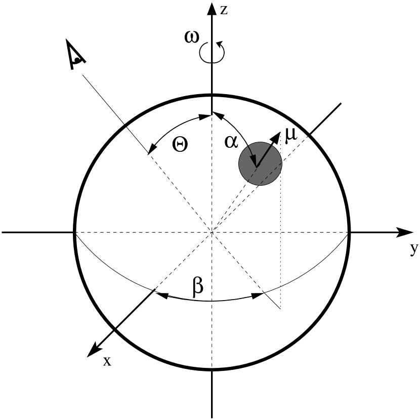
Figure 9.— Schematic view of the dipole model, indicating the different angles used to calculate the CRSF energy variation.$\beta$ is the angle between the projection of the magnetic moment in the x-y-plane and the ephemeris (x-axis) .The eye indicates the line of sight towards us.

The total average magnetic moment is divided into three components based on the cartesian coordinate system in Figure 9:

$$\mathbb{m}=\mu\begin{pmatrix}\text{sin}(\alpha)\text{cos}(\beta)\\ \text{sin}(\alpha)\text{sin}(\beta)\\ \text{sin}(\beta)\end{pmatrix}$$ (A2)

where $\alpha$ is the angle between the dipole field and the spin axis and $\beta$ is the rotation angle from the ephemeris, i.e. the x-axis. Next, the vector $\mathbb{n}$ was calculated for each individual phase bin $\phi$ used in the phase resolved analysis.

$$\mathbb{n}=\begin{pmatrix}\text{sin}(\Theta)\text{cos}(\phi)\\ \text{sin}(\Theta)\text{sin}(\phi)\\ \text{sin}(\phi)\end{pmatrix}$$ (A3)

The individual components of $\mathbb{n}$ are the projections of each phase bin on the three axes, as seen from the line of sight of the observer. The angle $\Theta$ corresponds to the angle between the line of sight and the spin axis. For each of the individual phase bins, the magnetic field was calculated using the position vector $\mathbb{n}$ indicating the position of the magnetic pole and the vector $\mathbb{m}$, which indicates the magnetic moment:

$$B_{\text{phase}}=\frac{3\cdot\mathbb{n}\left|\mathbb{m}\cdot\mathbb{n}\right|}{\left|\mathbb{n}\right|^{5}}-\frac{\mathbb{m}}{\left|\mathbb{n}\right|^{3}}$$ (A4)

The calculated magnetic field values were then fitted to the measured magnetic field, varying the three angles $\Theta$, $\alpha$, and $\beta$ until the best fit converged. To avoid wrong solutions due to local minima, the starting parameter of all three angles were varied in steps of $10^{\circ}$ before the fit was started. The best fit solutions resulted in the values that are discussed in detail in section 5.5.

References

- Basko & Sunyaev (1973) Basko, M. M., & Sunyaev, R. A., 1973, Ap&SS, 23, 117
- Basko & Sunyaev (1976) Basko, M. M., & Sunyaev, R. A., 1976, MNRAS, 175, 395
- Becker & Wolff (2007) Becker, P. A., & Wolff, M. T., 2007, Astrophys. J., 654, 435
- Braun & Yahel (1984) Braun, A., & Yahel, R. Z., 1984, ApJ, 278, 349
- Burderi et al. (2000) Burderi, L., Di Salvo, T., Robba, N. R., La Barbera, A., & Guainazzi, M., 2000, ApJ, 530, 429
- Coburn (2001) Coburn, W., 2001, Ph.D. thesis, UC San Diego
- Doroshenko et al. (2010a) Doroshenko, V., Santangelo, A., Suleimanov, V., Kreykenbohm, I., Staubert, R., Ferrigno, C., & Klochkov, D., 2010a, A&A, 515, A10
- Doroshenko et al. (2010b) Doroshenko, V., Suchy, S., Santangelo, A., Staubert, R., Kreykenbohm, I., Rothschild, R., Pottschmidt, K., & Wilms, J., 2010b, A&A, 515, L1
- Endo et al. (2002) Endo, T., Ishida, M., Masai, K., Kunieda, H., Inoue, H., & Nagase, F., 2002, ApJ, 574, 879
- Evangelista et al. (2010) Evangelista, Y., et al., 2010, ApJ, 708, 1663
- Fürst et al. (2011a) Fürst, F., Kreykenbohm, I., Suchy, S., Barragán, L., Wilms, J., Rothschild, R. E., & Pottschmidt, K., 2011a, A&A, 525, A73
- Fürst et al. (2011b) Fürst, F., Suchy, S., Kreykenbohm, I., Barragán, L., Wilms, J., Rothschild, R. E., & Pottschmidt, K., 2011b, A&A, in prep
- Göğüş, Kreykenbohm & Belloni (2011) Göğüş, E., Kreykenbohm, I., & Belloni, T. M., 2011, A&A, 525, L6+
- Jones, Chetin & Liller (1974) Jones, C. A., Chetin, T., & Liller, W., 1974, ApJ, 190, L1
- Kaastra & Mewe (1993) Kaastra, J. S., & Mewe, R., 1993, A&AS, 97, 443
- Kaper, van der Meer & Najarro (2006) Kaper, L., van der Meer, A., & Najarro, F., 2006, A&A, 457, 595
- Klochkov et al. (2008) Klochkov, D., et al., 2008, A&A, 482, 907
- Klochkov et al. (2011) Klochkov, D., Staubert, R., Santangelo, A., Rothschild, R. E., & Ferrigno, C., 2011, A&A, submitted
- Koh et al. (1997) Koh, D. T., et al., 1997, ApJ, 479, 933
- Kreykenbohm et al. (1999) Kreykenbohm, I., Kretschmar, P., Wilms, J., Staubert, R., Kendziorra, E., Gruber, D. E., Heindl, W. A., & Rothschild, R. E., 1999, A&A, 341, 141
- Kreykenbohm et al. (2004) Kreykenbohm, I., Wilms, J., Coburn, W., Kuster, M., Rothschild, R. E., Heindl, W. A., Kretschmar, P., & Staubert, R., 2004, A&A, 427, 975
- Kreykenbohm et al. (2008) Kreykenbohm, I., et al., 2008, A&A, 492, 511
- La Barbera et al. (2003) La Barbera, A., Santangelo, A., Orlandini, M., & Segreto, A., 2003, A&A, 400, 993
- La Barbera et al. (2005) La Barbera, A., Segreto, A., Santangelo, A., Kreykenbohm, I., & Orlandini, M., 2005, A&A, 438, 617
- Leahy (2002) Leahy, D. A., 2002, A&A, 391, 219
- Leahy & Kostka (2008) Leahy, D. A., & Kostka, M., 2008, MNRAS, 384, 747
- Lewin et al. (1971) Lewin, W. H. G., McClintock, J. E., Ryckman, S. G., & Smith, W. B., 1971, ApJ, 166, L69
- Matsumoto et al. (2006) Matsumoto, H., et al., 2006, in Society of Photo-Optical Instrumentation Engineers, Proc. SPIE, Vol. 6266
- McClintock, Ricker & Lewin (1971) McClintock, J. E., Ricker, G. R., & Lewin, W. H. G., 1971, ApJ, 166, L73
- Meszaros & Nagel (1985) Meszaros, P., & Nagel, W., 1985, ApJ, 299, 138
- Mihara (1995) Mihara, T., 1995, Ph.D. thesis, Univ. of Tokyo
- Mihara et al. (1990) Mihara, T., Makishima, K., Ohashi, T., Sakao, T., & Tashiro, M., 1990, Nature, 346, 250
- Mihara et al. (2007) Mihara, T., et al., 2007, Prog. Theor. Phys. Suppl., 169, 191
- Mitsuda et al. (2007) Mitsuda, K., et al., 2007, PASJ, 59, 1
- Mowlavi et al. (2006) Mowlavi, N., et al., 2006, A&A, 451, 187
- Mukherjee & Paul (2004) Mukherjee, U., & Paul, B., 2004, A&A, 427, 567
- Nakajima, Mihara & Makishima (2010) Nakajima, M., Mihara, T., & Makishima, K., 2010, ApJ, 710, 1755
- Orlandini et al. (2000) Orlandini, M., dal Fiume, D., Frontera, F., Oosterbroek, T., Parmar, A. N., Santangelo, A., & Segreto, A., 2000, Advances in Space Research, 25, 417
- Parkes et al. (1980) Parkes, G. E. and Culhane, J. L. and Mason, K. O. and Murdin, P. G., 1980, MNRAS, 454, 872
- Pravdo et al. (1995) Pravdo, S. H., Day, C. S. R., Angelini, L., Harmon, B. A., Yoshida, A., & Saraswat, P., 1995, ApJ, 191, 547
- Pravdo & Ghosh (2001) Pravdo, S. H., & Ghosh, P., 2001, ApJ, 554, 383
- Soong et al. (1990) Soong, Y., Gruber, D. E., Peterson, L. E., & Rothschild, R. E., 1990, ApJ, 348, 641
- Staubert et al. (2007) Staubert, R., Shakura, N. I., Postnov, K., Wilms, J., Rothschild, R. E., Coburn, W., Rodina, L., & Klochkov, D., 2007, A&A, 465, L25
- Suchy et al. (2011) Suchy, S., et al., 2011, ApJ, 733, 15
- Takahashi et al. (2007) Takahashi, T., et al., 2007, PASJ, 59, 35
- Tanaka (1986) Tanaka, Y., 1986, in Radiation Hydrodynamics in Stars and Compact Objects, ed. D. Mihalas & K.-H. A. Winkler, IAU Colloq. series 89, Vol. 255, 198
- Tsygankov et al. (2006) Tsygankov, S. S., Lutovinov, A. A., Churazov, E. M., & Sunyaev, R. A., 2006, MNRAS, 371, 19
- Tsygankov et al. (2007) Tsygankov, S. S., Lutovinov, A. A., Churazov, E. M., & Sunyaev, R. A., 2007, Astron. Lett., 33, 368
- Verner et al. (1996) Verner, D. A., Ferland, G. J., Korista, K. T., & Yakovlev, D. G., 1996, ApJ, 465, 487
- Watanabe et al. (2003) Watanabe, S., et al., 2003, ApJ, 597, L37
- White et al. (1976) White, N. E., Mason, K. O., Huckle, H. E., Charles, P. A., & Sanford, P. W., 1976, ApJ, 209, L119
- White, Mason & Sanford (1978) White, N. E., Mason, K. O., & Sanford, P. W., 1978, MNRAS, 184, 67P
- Wilms, Allen & McCray (2000) Wilms, J., Allen, A., & McCray, R., 2000, ApJ, 542, 914