Abstract

We find polarization modes of gravitational waves in topologically massive and new massive gravities by using the Newman-Penrose formalism where the null real tetrad is necessary to specify gravitational waves. The number of polarization modes is two for the new massive gravity and one for the topologically massive gravity, which is consistent with the metric-perturbation approach.

PACS numbers:

Typeset Using LaTeX

1 Introduction

Einstein gravity has been known to have no propagating degrees of freedom in three dimensions. Massive generalizations of the Einstein gravity may allow propagating degrees of freedom. Topologically massive gravity (TMG) is the famous gravity theory obtained by including a gravitational Chern–Simons term (gCS) with coupling $\mu$ [1, 2]. Since the gCS term is odd under parity, the theory shows a single massive propagating degree of freedom of a given helicity, whereas the other helicity mode remains massless. The model was extended by adding a cosmological constant $\Lambda=-1/\ell^{2}$ to the topologically massive gravity [3]. Then, the single massive field could be realized as a massive scalar $\varphi=z^{3/2}h_{zz}$ when employing the Poincare coordinates $x^{\pm}$ and $z$ covering the AdS₃ spacetimes [4]. It was shown that the massive graviton having negative-energy disappears at the chiral point of $\mu\ell=1$ by Lee-Song-Strominger in Ref. [5]. Furthermore, this cosmological topological massive gravity at the chiral point may be described by the logarithmic conformal field theory  [6, 7]. Importantly, the Lee-Song-Strominger work has indicated that the “third-order” Einstein equation turned out to be the “first-order” equation for a massive graviton when choosing the transverse-traceless gauge for metric tensor.

On the other hand, Bergshoeff, Hohm, and Townsend have recently proposed another massive generalization of the Einstein gravity by adding a specific quadratic curvature term to the Einstein-Hilbert action [8, 9]. This term was designed to reproduce the ghost-free Fierz-Pauli action for a massive propagating graviton in the linearized approximation, whereas it differs from the Fierz-Pauli term when considering the non-linear terms. This gravity theory became known as new massive gravity (NMG). Unlike the TMG, the NMG preserves parity. As a result, the gravitons acquire the same mass for both helicity states, indicating two massive propagating degrees of freedom. Considering TMG together with NMG leads to mass-splitting between helicity states.

So far, we have considered only the conventional metric-perturbation approach to three-dimensional massive gravities. Hence, we do not know explicitly what are polarization modes of gravitational waves (GW) in TMG and NMG. Since two massive theories belong to higher curvature gravity, we need to introduce the Newman-Penrose formalism [10] where the null real tetrad is necessary to specify polarization modes of GW, as the four-dimensional massive gravity requires null complex tetrad to specify six independent polarization modes of $\{\Phi_{2},\Psi_{3},\Psi_{4},\Phi_{22}\}$ [11]. Here $\Psi_{3}$ and $\Psi_{4}$ are complex, and analyzing the rotational behavior of the set shows the respective helicity values $s=\{0,\pm 1,\pm 2,0\}$. It was suggested that the observations of the GW will be done in the near future, and the corresponding determination of all possible states of polarization would be a very powerful test to rule out the present studied alternative theories of gravity.

In this work, we will find the polarization modes of gravitational waves arisen from the TMG and NMG by employing the the Newman-Penrose formalism in three dimensions. Even though these theories are not four-dimensional gravity theory, they will provide a prototype of polarization states. This work will be important to see how massive modes with different polarizations propagate in the three-dimensional Minkowski spacetimes. Since higher-order Einstein equation becomes lower-order equation when using the linearized Ricci tensor $R^{L}_{\mu\nu}$ instead of metric tensor $h_{\mu\nu}$, this work will provide another approach in addition to the conventional metric-perturbation theory.

2 Null real triad formalism in three dimensions

Let us first introduce a triad [12, 13] of real vectors $\{{\bf k},\bf{n},\bf{m}\}$ which are related to the Cartesian tetrad vectors $\{{\bf e}_{t},{\bf e}_{x},{\bf e}_{z}\}$ in three dimensions with metric signature $(-,+,+)$ as

$${\bf k}=\frac{1}{\sqrt{2}}({\bf e}_{t}+{\bf e}_{z}),~{}~{}{\bf n}=\frac{1}{\sqrt{2}}({\bf e}_{t}-{\bf e}_{z}),~{}~{}{\bf m}={\bf e}_{x},$$ (2.1)

where they satisfy the relations

$$-{\bf k}\cdot{\bf n}={\bf m}^{2}=1,~{}~{}~{}{\bf k}\cdot{\bf m}={\bf n}\cdot{\bf m}={\bf k}^{2}={\bf n}^{2}=0.$$ (2.2)

Note that a tensor ${\bf T}$ can be written as

$$T_{abc...}=T_{\mu\nu\rho...}a^{\mu}b^{\nu}c^{\rho_{...}},$$ (2.3)

where $(a,b,c,...)$ run over $({\bf k},\bf{n},\bf{m})$ and $(\mu,\nu,\rho,...)$ run over $(t,~{}x,~{}z)$. It is well-known that the Weyl tensor vanishes identically in three dimensions. Therefore, the Riemann tensor with six independent components can be decomposed into the Ricci tensor and Ricci scalar as

$$R_{\rho\sigma\mu\nu}=2\Big{(}g_{\rho[\mu}R_{\nu]\sigma}-g_{\sigma[\mu}R_{\nu]\rho}\Big{)}-Rg_{\rho[\mu}g_{\nu]\sigma}.$$ (2.4)

On the other hand, by using the formalism of real two-component spinors [13], the Ricci spinor $\Phi_{ABCD}$ can be expressed in terms of the Ricci tensor as

$$\Phi_{00} \equiv \Phi_{0000}=\frac{1}{2}R_{\mu\nu}k^{\mu}k^{\nu},$$

$$\Phi_{22} \equiv \Phi_{1111}=\frac{1}{2}R_{\mu\nu}n^{\mu}n^{\nu},$$

$$\Phi_{10} \equiv \Phi_{1000}=\frac{1}{2\sqrt{2}}R_{\mu\nu}m^{\mu}k^{\nu},$$

$$\Phi_{12} \equiv \Phi_{1011}=\frac{1}{2\sqrt{2}}R_{\mu\nu}m^{\mu}n^{\nu},$$

$$\Phi_{11} \equiv \Phi_{0011}=\frac{1}{6}\left(R_{\mu\nu}m^{\mu}m^{\nu}+R_{\mu\nu}n^{\mu}k^{\nu}\right).$$ (2.5)

Eardley et al.[11] have shown that polarization states of the GW in four dimensions can be given by six independent components of the Riemann tensor. They assumed that the GW are weak and take nearly plane waves propagating in the $+z$ direction. Accordingly, the GW have six independent modes which correspond to six independent Riemann tensor of the Newman-Penrose tetrad. Following the Eardley et al. approach, we consider the plane GW propagating in the $+z$ direction, which means that all quantities have the forms of $(t-z)$ only. This is equivalent to gauge-fixing (for example, transverse gauge) in the metric-perturbation approach. In this case, it is shown that the Riemann tensor satisfies the following relation

$$\partial_{p}R_{abcd}=0,$$ (2.6)

where $(a,b,c,d$) run over in $({\bf k},\bf{n},\bf{m})$ and $(p,q)$ run over $(\bf{k},{\bf m})$. Introducing a metric perturbation of $g_{\mu\nu}=\eta_{\mu\nu}+h_{\mu\nu}$ and the linearized Riemann tensor $R_{abcd}^{L}(h)$, the Bianchi identity can be written as

$$\nabla_{[n}R_{pq]ab}=0\Rightarrow\partial_{[n}R_{pq]ab}^{L} = \frac{1}{3}\left(\partial_{n}R_{pqab}^{L}+\partial_{p}R_{qnab}^{L}+\partial_{q}R_{npab}^{L}\right)$$ (2.7)

$$= \frac{1}{3}\partial_{n}R_{pqab}^{L}=0.$$

In deriving the second line, we have used the relation (2.6). Consequently, from Eq. (2.7), we have

$$R_{pqab}^{L}(h)={\rm const.},$$ (2.8)

which implies that the independent components of the Riemann tensor are given by three of $R_{pnqn}^{L}$ as

$$R_{knkn}^{L}(h),~{}~{}~{}R_{knmn}^{L}(h),~{}~{}~{}R_{mnmn}^{L}(h).$$ (2.9)

It is noted that three components (2.9) can be reexpressed in terms of the Ricci tensor in $\{{\bf k,n,m}\}$ basis like

$$R_{kn}^{L}(h),~{}~{}~{}~{}~{}R_{mn}^{L}(h),~{}~{}~{}~{}~{}R_{nn}^{L}(h)$$ (2.10)

which correspond to $\Phi_{11},~{}\Phi_{12},$ and $\Phi_{22}$ in (2.5), respectively.

Finally, we again point out that in three dimensions, the maximum number of polarization modes for GW is three of $R_{kn}^{L},~{}R_{mn}^{L}~{},$ and $R_{nn}^{L}$ (see Figure 1). In the next section we will investigate these modes by considering three gravity theories.

3 Massive gravities

We mention that the procedure of determining the number of the independent component of the Riemann tensor was done by choosing the plane wave solution to the vacuum linearized Einstein equation. This implies that the observer is far from GW sources, which means that it is enough to solve the vacuum linearized Einstein equation. In order to find polarization modes, we introduce three theories of the Einstein gravity, NMG and TMG. Before finding polarization modes from three theories, we wish to mention the three dimensional Fierz-Pauli (FP) massive equations which will be used to define the spin 2 in Sec.3.3 and 3.4.

3.1 FP massive equations

It is well known that the FP massive equations for a symmetric rank-$s$ tensor field describe the massive modes of helicity $\pm s$ with mass $m$. In three-dimensional Minkowski spacetimes, the FP massive equations are given by [14]

$$[{\cal D}(m){\cal D}(-m)]_{~{}\mu_{1}}^{\rho}\phi_{\rho\mu_{2}\cdots\mu_{s}}=0,~{}~{}~{}~{}\eta^{\mu\nu}\phi_{\mu\nu\rho_{1}\cdots\rho_{s-2}}=0.$$ (3.1)

Here the operator

$${\cal D}(m)_{\mu}^{\nu}=\frac{1}{2}\Big{[}\delta_{\mu}^{\nu}-\frac{1}{m}\epsilon_{\mu}^{~{}\rho\nu}\partial_{\rho}\Big{]}$$ (3.2)

is an on-shell projection operator as

$${\cal D}^{2}(m)\phi={\cal D}(m)\phi$$ (3.3)

if $\phi$ satisfies (3.1). In particular, if one considers the generalized massive gravity of NMG + gCS term, the parity-violating FP equations takes the form

$$[{\cal D}(m_{+}){\cal D}(-m_{-})]_{~{}\mu_{1}}^{\rho}\phi_{\rho\mu_{2}\cdots\mu_{s}}=0,~{}~{}~{}~{}\eta^{\mu\nu}\phi_{\mu\nu\rho_{1}\cdots\rho_{s-2}}=0$$ (3.4)

for two independent masses $m_{\pm}$. These equations show that one mode of helicity $s$ with mass $m_{+}$ and the other of helicity $-s$ with mass $m_{-}$ propagate. In this case, the second-order dynamical equation leads to

$$\left(\Box-m^{2}\right)\phi_{\mu_{1}\cdots\mu_{s}}=\tilde{\mu}\epsilon_{\mu_{1}}^{~{}~{}\rho\nu}\partial_{\rho}\phi_{\nu\mu_{2}\cdots\mu_{s}}$$ (3.5)

with

$$m^{2}=m_{+}m_{-},~{}~{}\tilde{\mu}\equiv m_{-}-m_{+}.$$ (3.6)

In the limit of $m_{-}\to\infty$ for fixed $m_{+}$, the helicity $-s$ mode decouples and thus, a single mode of helicity $s$ and mass $m_{+}$ is described by the first-order equation

$${\cal D}(\mu)_{~{}\mu_{1}}^{\rho}\phi_{\rho\mu_{2}\cdots\mu_{s}}=0,~{}~{}~{}~{}\eta^{\mu\nu}\phi_{\mu\nu\rho_{1}\cdots\rho_{s-2}}=0,$$ (3.7)

where $\mu=m^{2}/\tilde{\mu}$. Let us confine ourselves to spin 2, and consider the self-dual spin 2 model with field equation

$${\cal D}(\mu)^{\rho}_{~{}\mu}\phi_{\rho\nu}=0,~{}~{}\eta^{\mu\nu}\phi_{\mu\nu}=0$$ (3.8)

and the subsidiary condition $\partial^{\mu}\phi_{\mu\nu}=0$. The general solution is given by

$$\phi_{\mu\nu}={\cal G}^{\rho\sigma}_{\mu\nu}h_{\rho\sigma}\equiv G^{\rm L}_{\mu\nu},~{}~{}{\cal G}^{\rho\sigma}_{\mu\nu}=-\frac{1}{2}\epsilon_{(\mu}^{~{}~{}\eta\rho}\epsilon_{\nu)}^{~{}~{}\tau\sigma}\partial_{\eta}\partial_{\tau}$$ (3.9)

for some second-rank tensor $h_{\mu\nu}$. Here $G^{L}_{\mu\nu}$ is the linearized Einstein tensor for the metric perturbation of $g_{\mu\nu}=\eta_{\mu\nu}+h_{\mu\nu}$. Then, the self-dual field equation of (3.8) becomes

$${\cal D}(\mu)^{\rho}_{~{}\mu}G^{L}_{\rho\nu}=0,~{}~{}\eta^{\mu\nu}G^{L}_{\mu\nu}=0$$ (3.10)

which implies the linearized Einstein equation for the TMG. This confirms the equivalence of the linearized TMG to the self-dual spin 2 theory in three dimensions.

Similarly, we check that the FP massive equation

$$[{\cal D}(m){\cal D}(-m)]_{~{}\mu}^{\rho}\phi_{\rho\nu}=0,~{}~{}~{}~{}\eta^{\mu\nu}\phi_{\mu\nu}=0$$ (3.11)

is equivalent to the linearized equations for the NMG

$$[{\cal D}(m){\cal D}(-m)]_{~{}\mu}^{\rho}G^{L}_{\rho\nu}=0,~{}~{}R^{L}=0.$$ (3.12)

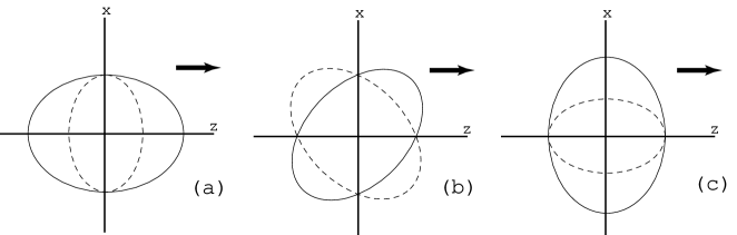
Figure 1: Three polarization modes of weak, plane GW permitted in three-dimensional massive gravity. The displacement shows that each mode induces on a sphere of test particles, i.e., $(a):~{}\Phi_{11}=\frac{1}{6}R_{kn}=\frac{1}{6}R_{ztzt},~{}(b):~{}\Phi_{12}=\frac{1}{2\sqrt{2}}R_{mn}=\frac{1}{2}R_{xtzt},~{}(c):~{}\Phi_{22}=~{}\frac{1}{2}R_{nn}=R_{xtxt}$. In this figure all waves are propagating in the $+z$ direction.

3.2 Einstein gravity

The Einstein-Hilbert action with a matter term is given by

$$S_{EH}=\frac{1}{16\pi G}\int d^{3}x\sqrt{-g}R+S_{m},$$ (3.13)

which yields the Einstein equation

$$G_{\mu\nu}=8\pi GT_{\mu\nu},~{}~{}~{}G_{\mu\nu}=R_{\mu\nu}-\frac{R}{2}g_{\mu\nu}.$$ (3.14)

In the case of $T_{\mu\nu}=0$, we obtain $R_{\mu\nu}=0$. Considering the metric perturbation of $g_{\mu\nu}=\eta_{\mu\nu}+h_{\mu\nu}$, the linearized equation becomes

$$R_{\mu\nu}^{L}(h)=0.$$ (3.15)

Using the relation (2.3) between $(\mu,\nu,\rho,...)$ and $(a,b,c,...)$, one shows that $R_{\mu\nu}^{L}=0$ correspond to

$$R_{kn}^{L}=R_{mn}^{L}=R_{nn}^{L}=0\to\Phi_{11}=\Phi_{12}=\Phi_{22}=0.$$ (3.16)

This indicates that there is no propagating mode of the GW in Einstein gravity. However, the result is nothing new because the linearized second-order equation for $h_{\mu\nu}$ implies no graviton in three dimensions [15]. We would like to mention that the Newman-Penrose approach confirms the result of the metric-perturbation approach.

3.3 NMG

In NMG [16] proposed by Bergshoeff, Hohm, and Townsend, the action is given by

$$S_{\rm NMG}=\frac{1}{\kappa^{2}}\int d^{3}x\sqrt{-g}\Big{(}-R+\alpha R^{2}+\beta R_{\mu\nu}R^{\mu\nu}\Big{)},$$ (3.17)

where the constant $\kappa$ has the mass dimension $[\kappa]=-1/2$, and $\alpha$ and $\beta$ are dimensionless constants satisfying the important relation of $\alpha=-3\beta/8$ which kills the spin-0 mode (scalar graviton). The wrong sign in the Einstein-Hilbert term is necessary to avoid the ghost. From the action (3.17), the equation of motion for the metric can be derived as

$$G_{\mu\nu}-\alpha\Big{[}2RG_{\mu\nu}+2g_{\mu\nu}\nabla_{\gamma}\nabla^{\gamma}R-2\nabla_{\mu}\nabla_{\nu}R\Big{]}$$

$$-\beta\Big{[}-\frac{1}{2}g_{\mu\nu}R_{\rho\sigma}R^{\rho\sigma}+2R_{\mu\rho\nu\sigma}R^{\rho\sigma}+\nabla_{\gamma}\nabla^{\gamma}R_{\mu\nu}+\frac{1}{2}g_{\mu\nu}\nabla_{\gamma}\nabla^{\gamma}R-\nabla_{\mu}\nabla_{\nu}R\Big{]}=0.$$ (3.18)

Considering the metric perturbation $g_{\mu\nu}=\eta_{\mu\nu}+h_{\mu\nu}$, the linearized equation takes the form

$$\square R_{\mu\nu}^{L}-\frac{1}{\beta}R_{\mu\nu}^{L}=0,~{}~{}\square=\partial_{\gamma}\partial^{\gamma}$$ (3.19)

which is interpreted as the second-order equation for $R^{L}_{\mu\nu}$. This means that the fourth-order equation for $h_{\mu\nu}$ could be interpreted as the second-order equation for $R^{L}_{\mu\nu}(h)=-\frac{1}{2}\square h^{TT}_{\mu\nu}$ with transverse-traceless (TT) gauge. In deriving this, we have used the perturbation equation for the trace of Eq.(3.3) like

$$R^{L}=0$$ (3.20)

together with $8\alpha+3\beta=0$. It is important to note that Eq.(3.19) is exactly the same with the second-order dynamical equation (3.5) with $m_{+}=m_{-}=m$ when replacing $\phi_{\mu\nu}\Leftrightarrow R_{\mu\nu}^{L}$ and $m\Leftrightarrow\frac{1}{\sqrt{\beta}}$. This implies that Eq.(3.19) describes the massive modes of helicity $\pm 2$ with mass $1/\sqrt{\beta}$.

Furthermore, the solution to Eq.(3.19) is given by

$$R_{\mu\nu}^{L}=M_{\mu\nu}e^{ip\cdot x},$$ (3.21)

where $p^{2}=-1/\beta$ and $M_{\mu\nu}$ is a constant symmetric tensor which satisfies to the following conditions:

$$M^{\mu}_{\mu}=0,~{}~{}~{}p^{\mu}M_{\mu\nu}=0.$$ (3.22)

From (2.3) and the Ricci scalar in $\{{\bf k,n,m}\}$ basis, we find that Eqs.(3.20) and (3.21) correspond to

$$R_{kn}^{L}=0~{}~{}~{}{\rm and}~{}~{}~{}R_{mn}^{L}\neq 0,~{}~{}R_{nn}^{L}\neq 0,$$ (3.23)

respectively. This shows that the number of polarization modes of GW in the NMG is two of $R_{mn}^{L}\to\Phi_{12}$ and $R_{nn}^{L}\to\Phi_{22}$. Interestingly, as was shown in [16], two propagating modes appear in the NMG. It is worth noting that in our approach, $R_{kn}^{L}=0$ implies that there is no ghost-like massive mode of zero helicity because of $R_{kn}^{L}=R^{L}=0$. In addition, $R_{mn}^{L}$ and $R_{nn}^{L}$ correspond to the TT  metric-perturbation theory. Their two polarization modes are depicted in $(b)$ and $(c)$ of Fig. 1.

On the other hand, we may consider the general case of $8\alpha+3\beta\neq 0$. In this case, instead of Eqs.(3.19) and (3.20), we obtain

$$R_{\mu\nu}^{L}-\beta\square R_{\mu\nu}^{L}+(2\alpha+\beta)\partial_{\mu}\partial_{\nu}R^{L}+(2\alpha+\beta)\eta_{\mu\nu}\square R^{L} = 0,$$ (3.24)

$$(8\alpha+3\beta)\square R^{L}+R^{L} = 0.$$ (3.25)

The solutions for the above equations are obtained by

$$R^{L}=R_{0}e^{iq\cdot x},~{}~{}~{}R_{\mu\nu}^{L}=N_{\mu\nu}e^{iq\cdot x},$$ (3.26)

where $q^{2}=1/(8\alpha+3\beta)$ and $N_{\mu\nu}$ is a constant symmetric tensor given by

$$N_{\mu\nu}=\frac{8\alpha+3\beta}{4}\left(q_{\mu}q_{\nu}-\frac{\eta_{\mu\nu}}{8\alpha+3\beta}\right)R_{0}.$$ (3.27)

We see that in $\{{\bf k,n,m}\}$ basis, the solution (3.26) corresponds to

$$R_{kn}^{L}\neq 0,~{}~{}~{}~{}~{}R_{mn}^{L}\neq 0,~{}~{}~{}~{}~{}R_{nn}^{L}\neq 0,$$ (3.28)

which mean that there exist three independent polarization modes ($\Phi_{11},\Phi_{12},\Phi_{22}$) in the NMG with $8\alpha+3\beta\neq 0$. Their three polarization modes are depicted in $(a)$, $(b)$, and $(c)$ of Fig. 1.

3.4 TMG

The TMG was first proposed by Deser, Jackiw, and Templeton [17, 18] in the aim of making the massive gravity theory in three dimensions. The TMG action takes the form

$$S_{TMG}=-\frac{1}{\kappa^{2}}\int d^{3}x\sqrt{-g}R-\frac{1}{\mu\kappa^{2}}S_{CS},$$ (3.29)

where $\mu$ is the gCS coupling constant and $S_{CS}$ is the gCS term,

$$S_{CS}=\frac{1}{2}\int d^{3}x\sqrt{-g}\epsilon^{\lambda\mu\nu}\Gamma_{\lambda\sigma}^{\rho}\Big{(}\partial_{\mu}\Gamma_{\rho\nu}^{\sigma}+\frac{2}{3}\Gamma_{\mu\tau}^{\sigma}\Gamma_{\nu\rho}^{\tau}\Big{)}.$$ (3.30)

The wrong sign in the Einstein-Hilbert term is necessary to avoid the ghost. Varying the action (3.29) with respect to the metric yields

$$G_{\mu\nu}+\frac{1}{\mu}C_{\mu\nu}=0,$$ (3.31)

where $C_{\mu\nu}$ is the Cotton tensor defined by

$$C_{\mu\nu}\equiv\epsilon_{\mu}^{~{}\alpha\beta}\nabla_{\alpha}\left(R_{\beta\nu}-\frac{1}{4}g_{\beta\nu}R\right).$$ (3.32)

One finds that taking the trace of Eq.(3.31) leads to $R=0$. Substituting $R=0$ into Eq.(3.31), the linearized equation can be written by

$$R_{\mu\nu}^{L}=-\frac{1}{\mu}\eta_{\mu\rho}\epsilon^{\rho\alpha\beta}\partial_{\alpha}R_{\beta\nu}^{L}$$ (3.33)

which leads to (3.10) when replacing $\mu$ by $-\mu$. Importantly, we point out that Eq.(3.33) is the third-order equation for $h_{\mu\nu}$, whereas it is regarded as the first-order equation for $R^{L}_{\mu\nu}=-\frac{1}{2}\square h_{\mu\nu}^{TT}$. It is interesting to note that Eq.(3.33) is equivalent to the self-dual model with (3.8) when replacing $\phi_{\mu\nu}\Leftrightarrow R_{\mu\nu}^{L}$ and $\mu\Leftrightarrow-\mu$. Apparently, from Eq. (3.33) and $R^{L}=0$, we expect that the independent components of the Riemann tensor is two of $R_{mn}^{L}$ and $R_{nn}^{L}$, as was shown in the NMG. However, we have to check whether $R_{mn}^{L}$ and $R_{nn}^{L}$ are truly independent components even though we do not know the exact solution. To this end, we note that there are mixing between components of the Ricci tensor in Eq.(3.33) because of the Livi-Civita tensor $\epsilon^{\rho\alpha\beta}$. From the $(t,t),~{}(t,z),$ and $(z,z)$ components of Eq.(3.33), we obtain one first-order equation (see Appendix for details):

$$\partial_{x}\Big{(}R_{tt}^{L}+2R_{tz}^{L}+R_{zz}^{L}\Big{)}-\mu\Big{(}R_{tt}^{L}+2R_{tz}^{L}+R_{zz}^{L}\Big{)}=(\partial_{t}+\partial_{z})\Big{(}R_{tx}^{L}+R_{xz}^{L}\Big{)},$$ (3.34)

which implies that $R_{tt}^{L}+2R_{tz}^{L}+R_{zz}^{L}$ and $R_{tx}^{L}+R_{xz}^{L}$ are not independent. Using the $\{{\bf k,n,m}\}$ basis, this indicates that $R_{mn}^{L}$ and $R_{nn}^{L}$ are not independent because $R_{mn}^{L}=-\left(R_{tx}^{L}+R_{xz}^{L}\right)/\sqrt{2}$ and $R_{nn}^{L}=\left(R_{tt}^{L}+2R_{tz}^{L}+R_{zz}^{L}\right)/2$.

Finally, we conclude that there exists one independent mode of GW in the TMG. If one chooses the positive gCS coupling with $\mu>0$, its mode is $R_{nn}^{L}=\Phi_{22}$, while for $\mu<0$, its mode is $R_{mn}^{L}=\Phi_{12}$ or vice versa.

4 Discussions

We have found polarization modes of gravitational waves in topologically massive and new massive gravities by using the Newman-Penrose formalism. As was shown in Fig. 1, the number of polarization modes is two [$(b)$ and $(c)$] for the new massive gravity and one [$(b)$ or $(c)$] for the topologically massive gravity. In order to obtain the explicit mode shape, we note that the linearized equation is equivalent to the FP massive equations which define the massive spin 2 field in three dimensions. Then, using the Newman-Penrose formalism, we obtain all polarization modes of NMG and TMG. As far as we know, this work firstly shows what kind of massive modes are propagating in the three-dimensional Minkowski spacetimes.

Some people have considered the TMG and the NMG as toy models of quantum gravity because they are free from the tachyon and ghosts in the metric-perturbation approach. Furthermore, it was shown that the NMG is free from the non-linear ghost (Boulware-Deser ghost) to any order beyond the decoupling limit [19]. It shows really that the NMG represents a completely consistent ghost free theory of a fully interacting massive graviton in three dimensions [20]. It was claimed that this theory is renormalizable [21]. On the contrary, this theory seems not be renormalizable because the scalar graviton killed by choosing $\alpha=-3\beta/8$ is necessary to achieve the renormalizability [22]. Actually, the unitarity and renormalizability exclude to each other [23]. At this stage, we do not have any definite answer to the renormalizability of the NMG.

On the other hand, the relevant quantity to specify polarization modes is not the metric tensor $h_{\mu\nu}$ but the linearized Ricci tensor $R^{L}_{\mu\nu}$ (equivalently, the linearized Einstein tensor $G^{L}_{\mu\nu}$ with $R^{L}=0$). If one considers $R^{L}_{\mu\nu}$ as the physical quantity, the fourth-order linearized Einstein equation for $h_{\mu\nu}$ reduces to the second-order equation for $R^{L}_{\mu\nu}$, which is exactly the self-dual field equation of the FP massive equation. The latter defines the spin of massive modes. In this sense, the NMG and TMG are considered as models of truly massive gravity in three dimensions. These two theories reflect how the lower-dimensional gravity could be realized only as massive gravity theory because the Einstein gravity is trivial in three dimensions. The only and nontrivial way to provide the spin 2 field is to use the linearized Ricci tensor through the Newman-Penrose formalism. Hence, the TMG becomes the first-order theory and the NMG is the second-order theory, even though they of TMG and NMG are third- and fourth-order theory in the metric-perturbation approach.

Acknowledgments

This work was supported by the National Research Foundation of Korea (NRF) grant funded by the Korea government (MEST) through the Center for Quantum Spacetime (CQUeST) of Sogang University with Grant No.2005-0049409. Y. Myung was partly supported by the National Research Foundation of Korea (NRF) grant funded by the Korea government (MEST) (No.2011-0027293).

Appendix: The linearized perturbation equations in the TMG

The explicit forms of linearized equation (3.33) are given by

$$R_{tt}^{L} = \frac{1}{\mu}\left(\partial_{x}R_{zt}^{L}-\partial_{z}R_{xt}^{L}\right)$$

$$R_{tx}^{L} = \frac{1}{\mu}\left(\partial_{x}R_{zx}^{L}-\partial_{z}R_{xx}^{L}\right)~{}~{}{\rm or}~{}~{}\frac{1}{\mu}\left(\partial_{x}R_{zt}^{L}-\partial_{z}R_{xt}^{L}\right)$$

$$R_{tz}^{L} = \frac{1}{\mu}\left(\partial_{x}R_{zz}^{L}-\partial_{z}R_{xz}^{L}\right)~{}~{}{\rm or}~{}~{}\frac{1}{\mu}\left(\partial_{x}R_{tt}^{L}-\partial_{t}R_{xt}^{L}\right)$$

$$R_{xx}^{L} = \frac{1}{\mu}\left(\partial_{t}R_{zx}^{L}-\partial_{z}R_{xt}^{L}\right)$$

$$R_{xz}^{L} = \frac{1}{\mu}\left(\partial_{t}R_{zz}^{L}-\partial_{z}R_{tz}^{L}\right)~{}~{}{\rm or}~{}~{}\frac{1}{\mu}\left(\partial_{x}R_{tx}^{L}-\partial_{t}R_{xx}^{L}\right)$$

$$R_{zz}^{L} = \frac{1}{\mu}\left(\partial_{x}R_{tz}^{L}-\partial_{t}R_{xz}^{L}\right)$$

where $\epsilon^{txz}=1$ and the second terms of the r.h.s. in $R_{tx}^{L},~{}R_{tz}^{L},$ and $R_{xz}^{L}$ come from the Bianchi identity of $\partial^{\mu}\left(R_{\mu\nu}^{L}-\eta_{\mu\nu}R^{L}/2\right)=0$.

References

- [1] S. Deser, R. Jackiw and S. Templeton, Phys. Rev. Lett. 48, 975 (1982).
- [2] S. Deser, R. Jackiw and S. Templeton, Annals Phys. 140, 372 (1982) [Erratum-ibid. 185, 406 (1988)] [Annals Phys. 281, 409 (2000)].
- [3] S. Deser, in Quantum Theory of Gravity, edited by S.M. Christensen (Adam Hilger, London, 1984).
- [4] S. Carlip, S. Deser, A. Waldron and D. K. Wise, Class. Quant. Grav. 26, 075008 (2009) [arXiv:0803.3998 [hep-th]].
- [5] W. Li, W. Song and A. Strominger, JHEP 0804, 082 (2008) [arXiv:0801.4566 [hep-th]].
- [6] D. Grumiller and N. Johansson, JHEP 0807, 134 (2008) [arXiv:0805.2610 [hep-th]].
- [7] Y. S. Myung, Phys. Lett. B 670, 220 (2008) [arXiv:0808.1942 [hep-th]].
- [8] E. A. Bergshoeff, O. Hohm and P. K. Townsend, Phys. Rev. Lett. 102, 201301 (2009) [arXiv:0901.1766 [hep-th]].
- [9] E. A. Bergshoeff, O. Hohm and P. K. Townsend, Phys. Rev. D 79, 124042 (2009) [arXiv:0905.1259 [hep-th]].
- [10] E. Newman and R. Penrose, J. Math. Phys. 3, 566 (1962).
- [11] D. M. Eardley, D. L. Lee, A. P. Lightman, Phys. Rev. D8, 3308-3321 (1973).
- [12] G. S. Hall, T. Morgan and Z. Perjes, Gen. Rel. Grav. 19, 1137 (1987).
- [13] F. C. Sousa, J. B. Fonseca, C. Romero, Class. Quant. Grav. 25, 035007 (2008) [arXiv:0705.0758 [gr-qc]].
- [14] E. A. Bergshoeff, O. Hohm and P. K. Townsend, Annals Phys. 325, 1118 (2010) [arXiv:0911.3061 [hep-th]].
- [15] S. Deser, R. Jackiw, G. ’t Hooft, Annals Phys. 152, 220 (1984).
- [16] E. A. Bergshoeff, O. Hohm, P. K. Townsend, Phys. Rev. Lett. 102, 201301 (2009) [arXiv:0901.1766 [hep-th]].
- [17] S. Deser, R. Jackiw, S. Templeton, Phys. Rev. Lett. 48, 975-978 (1982).
- [18] S. Deser, R. Jackiw, S. Templeton, Annals Phys. 140, 372-411 (1982).
- [19] C. de Rham, G. Gabadadze, D. Pirtskhalava, A. J. Tolley and I. Yavin, JHEP 1106, 028 (2011) [arXiv:1103.1351 [hep-th]].
- [20] K. Hinterbichler, arXiv:1105.3735 [hep-th].
- [21] I. Oda, JHEP 0905, 064 (2009) [arXiv:0904.2833 [hep-th]].
- [22] K. S. Stelle, Phys. Rev. D 16, 953 (1977).
- [23] E. A. Bergshoeff, O. Hohm, P. K. Townsend, Cosmology, the Quantum Vacuum and Zeta Functions: A Workshop with a Celebration of Emilio Elizalde’s Sixtieth Birthday 2010, Bellaterra, Barcelona, Spain.