Prospect for Charge Current Neutrino Interactions Measurements at the CERN-PS

The NESSiE Collaboration

P. Bernardini^8,7, A. Bertolin¹⁰, C. Bozza¹³, R. Brugnera^11,10, A. Cecchetti⁵, S. Cecchini³, G. Collazuol^11,10, F. Dal Corso¹⁰, I. De Mitri^8,7 M. De Serio¹, D. Di Ferdinando³, U. Dore¹², S. Dusini¹⁰, P. Fabbricatore⁶, C. Fanin¹⁰, R. A. Fini¹, A. Garfagnini^11,10, G. Grella¹³, U. Kose¹⁰, M. Laveder^11,10, P. Loverre¹², A. Longhin⁵, G. Marsella^9,7 G. Mancarella^8,7 G. Mandrioli³, N. Mauri⁵, E. Medinaceli^11,10, M. Mezzetto¹⁰,
M. T. Muciaccia^2,1, D. Orecchini⁵, A. Paoloni⁵, A. Pastore^2,1, L. Patrizii³, M. Pozzato^4,3, R. Rescigno¹³, G. Rosa¹², S. Simone^2,1, M. Sioli^4,3, G. Sirri³, M. Spurio^4,3, L. Stanco^10,a, S. Stellacci¹³, A. Surdo⁷, M. Tenti^4,3, and V. Togo³.

1. INFN-Bari, 70126 Bari, Italy
2. Dipartimento di Fisica dell’Università di Bari, 70126 Bari, Italy
3. INFN-Bologna, 40127 Bologna, Italy
4. Dipartimento di Fisica dell’Università di Bologna, 40127 Bologna, Italy
5. Laboratori Nazionali di Frascati dell’INFN, 00044 Frascati (Roma), Italy
6. INFN-Genova, 16146 Genova, Italy
7. INFN-Lecce, 70126 Lecce, Italy
8. Dipartimento di Fisica dell’Università del Salento, 73100 Lecce, Italy
9. Dipartimento di Ingegneria dell’Innovazione dell Università del Salento, 73100 Lecce, Italy
10. INFN-Padova, 35131 Padova, Italy
11. Dipartimento di Fisica dell’Università di Padova, 35131 Padova, Italy
12. Dipartimento di Fisica dell’Università di Roma “La Sapienza” and INFN, 00185 Roma, Italy
13. Dipartimento di Fisica dell’Università di Salerno and INFN, 84084 Fisciano, Salerno, Italy
a  Contact Person

1 Introduction

Tensions in several phenomenological models grew with experimental results on neutrino/antineutrino oscillations at Short-Baseline (SBL) and with the recent, carefully recomputed, antineutrino fluxes from nuclear reactors. At a refurbished SBL CERN-PS facility an experiment aimed to address the open issues has been proposed [1], based on the technology of imaging in ultra-pure cryogenic Liquid Argon (LAr).

Motivated by this scenario a detailed study of the physics case was performed. We tackled specific physics models and we optimized the neutrino beam through a full simulation. Experimental aspects not fully covered by the LAr detection, i.e. the measurements of the lepton charge on event-by-event basis and their energy over a wide range, were also investigated. Indeed the muon leptons from Charged Current (CC) (anti-)neutrino interactions play an important role in disentangling different phenomenological scenarios provided their charge state is determined. Also, the study of muon appearance/disappearance can benefit of the large statistics of CC muon events from the primary neutrino beam.

Results of our study are reported in detail in this proposal. We aim to design, construct and install two Spectrometers at “NEAR” and “FAR” sites of the SBL CERN-PS, compatible with the already proposed LAr detectors. Profiting of the large mass of the two Spectrometers their stand-alone performances have also been exploited.

Some important practical constraints were assumed in order to draft the proposal on a conservative, manageable basis, and maintain it sustainable in terms of time-scale and cost. Well known technologies were considered as well as re-using parts of existing detectors (should they become available; if not it would imply an increase of the costs with no additional delay).

The momentum and charge state measurements of muons in a wide energy range, from few hundreds $MeV$ to several $GeV$, over a $>\ 50\ m^{2}$ surface, is an extremely challenging task if constrained by a 10 (and not 100) millions € budget for construction and installation. Running costs have to be kept at low level, too.

The experiment is identified throughout the proposal with the acronym NESSiE (Neutrino Experiment with SpectrometerS in Europe).

In the next Section the relevant physics pleas for the Spectrometer proposal are summarized. In Section 3 an extensive discussion of the physics case and the possible phenomenological models are described. In Section 4 details of a complete new simulation of the beam fluxes and horn designs are reported to work out a realistic situation and to be possibly used as contribution to the eventual design study group. In Section 5 the choice and design of the Spectrometers are discussed. After a brief reminder of the details of the Monte Carlo simulation for neutrino events (Section 6) the obtained physics performances are outlined in Section 7. Sections 8 and  9 deal with the technical definition of the mechanical structure and electrical setting-up for the magnets. Sections 10 and  11 show the use of possible detectors either with a coarse resolution ($\sim$1 $cm$) or with a boosted one ($\sim$1 $mm$). Section 12 debates about background levels to be taken into account for the data taking, described in Section 13. The last two sections report about CERN setting-up, schedule and costs. Finally conclusions are recapped.

2 Aims and Landmarks

The main physics topic of a new SLB CERN-PS experiment is to confirm or reject the so called neutrino anomalies and in case of a positive signal fully exploit the new physics connected with sterile neutrinos. The reported anomalies are the $\overline{\nu}_{\mu}\rightarrow\overline{\nu}_{e}$ transitions observed by LSND [2], the $\nu_{e}$ disappearance claimed by the Gallium source experiments for the Gallium solar neutrino reactions [3] and the $\overline{\nu}_{e}$ disappearance of reactor antineutrinos [4].

If such anomalies are not connected with new physics the LAr plus Spectrometer experiments will report null signal in the $\nu_{e}$ and $\overline{\nu}_{e}$ spectra, both in the absolute flux and energy shape, ruling out the anomalies at exceeding $\sigma$’s. In fact as in some sterile neutrino models, discussed in the following, cancellations occur between $\nu_{e}$ ($\overline{\nu}_{e}$) appearance, via $\overline{\nu}_{\mu}\rightarrow\overline{\nu}_{e}$ transitions and $\nu_{e}$ ($\overline{\nu}_{e}$) disappearance, a null result in the $\nu_{e}$ sector by LAr experiments would not be sufficient to fully exclude sterile neutrino models. In this case it will be crucial to precisely measure $\nu_{\mu}$ disappearance since it would be impossible for any model to fit both null results in the $\nu_{e}$ and the $\nu_{\mu}$ sectors.

We note that the best limit available so far on $\nu_{\mu}$ disappearance in the $\Delta m^{2}$ range under study, published by CDHS [5], is based on the analysis of 3300 events at the Far detector, corresponding to just one day of data taking of the experiment we propose.

We therefore clinch that in case of null signal the conjunct experiments will be able to rule out all the existing anomalies as connected to the presence of sterile neutrinos.

If instead the anomalies are really hints of the existence of sterile neutrinos the experiments will be able to:

• provide a direct signature of non-sterile neutrinos through the detection of Neutral Current (NC) disappearance. In fact while CC disappearance may occur via active neutrino oscillations, NC disappearance can only occur when active neutrinos oscillate to sterile ones. It goes without saying that NC disappearance should be at the same rate of $\nu_{\mu}$ charged current disappearance rate as measured by a spectrometer

  .

• Characterize the sterile neutrino model, namely to determine:

  • all the parameters of 3+1 models (3 parameters: $U_{4e}$, $U_{4\mu}$, $\Delta m^{2}_{14}$) or 3+2 models (7 parameters: $U_{4e}$, $U_{4\mu}$, $\Delta m^{2}_{14}$, $U_{5e}$, $U_{5\mu}$, $\Delta m^{2}_{15}$, $\Delta_{s}$);

  • the number of steriles from the number of $\Delta m^{2}$ needed to fit the data that will correspond to $\nu_{\mu}\rightarrow\nu_{e}$, $\overline{\nu}_{\mu}\rightarrow\overline{\nu}_{e}$ appearances and $\nu_{\mu}$ disappearance. Furthermore any manifestation of CP violation will be an evidence of at least 2 sterile neutrinos participating to oscillations.

  • CP violation in the sterile sector from the comparison of $\nu_{\mu}\rightarrow\nu_{e}$ and $\overline{\nu}_{\mu}\rightarrow\overline{\nu}_{e}$ transitions.

Therefore in case sterile neutrinos indeed exist the experiments will fully exploit the very rich and exciting physics information related to them.

From this concise discussion that will be more extensively addressed in the following, it clearly appears that a spectrometer capable of measuring the muon momenta would complement the LAr experiment by allowing to:

• measure $\nu_{\mu}$ disappearance in the entire available momentum range. This is a key information in rejecting/observing the anomalies over the whole expected parameter space of sterile neutrino oscillations;

• measure the neutrino flux at the Near detector, in the full muon momentum range, which is decisive to keep the systematic errors at the lowest possible values.

The measurement of the sign of the muon charge would furthermore enable to:

• separate $\nu_{\mu}$ from $\overline{\nu}_{\mu}$ in the antineutrino beam where the $\nu_{\mu}$ contamination is relevant. Such a measure is crucial for a firm observation of any difference between $\nu_{\mu}\rightarrow\nu_{e}$ and $\overline{\nu}_{\mu}\rightarrow\overline{\nu}_{e}$ transitions, a possible signature of CP violation;

• and finally reduce the data taking period by a concurrent collection of both $\nu_{\mu}$ and $\overline{\nu}_{\mu}$ events.

3 Physics

3.1 Introduction

The recent re-computation of antineutrino fluxes from nuclear reactors [4] leds to the so called “reactor neutrino anomaly” [6, 7], i.e. a $\sim$ 3% deficit of the reactor antineutrino rates measured at short baselines by past reactor experiments, reinforcing the case of sterile neutrinos.

The latest fits of cosmological parameters are in favor of a number of neutrinos above 3 (see e.g. [8]), provided that masses of extra neutrinos are below $\sim$1 $eV/c^{2}$ [9].

Besides reactor antineutrinos [7, 10] and cosmology, sterile neutrinos were invoked to explain results from beam dump experiments, LSND [2], accelerator neutrinos (and antineutrinos) as measured by the MiniBooNE experiment [11, 12] and source calibration data of the Gallium solar neutrino experiments [3]. Global fits to neutrino oscillation data [13] are performed by adding just one sterile neutrino to the three active, “3+1” models, or adding two sterile neutrinos, “3+2”. The latter models (see Fig. 1) provide a reasonable good fit to the data. In particular “3+2” models can introduce CP violation in the sterile sector, explaining the discrepancy between the $\overline{\nu}_{e}$ appearance detected by the LSND and the lack of $\nu_{e}$ appearance as reported by MiniBooNE. “3+1” models cannot introduce CP violation and when compared to “3+2” they are disfavored at 97.2% C.L. according to [13]. A way-out to improve the goodness of fit of the “3+1” model is to introduce the CPT violation [14].

Global fits do not provide a clear unique solution emerging from the data. Furthermore it should be noted that tension still exists between appearance and disappearance data [13]; for this reason even “3+2” global fits are not fully satisfactory.

In this Section we set the physics case of an accelerator neutrino experiment aiming at being the conclusive one on this topic. We recall the capabilities of a LAr detector and we focus on the physics opportunities that a spectrometer could add to a liquid argon target. We first discuss measures like the LSND/MiniBooNE evidence of $\overline{\nu}_{\mu}\rightarrow\overline{\nu}_{e}$ transitions and the $\nu_{e}$, $\overline{\nu}_{e}$ disappearances, as well as measures like $\nu_{\mu}$, $\overline{\nu}_{\mu}$ disappearances. Then the possible signatures of sterile neutrinos, including NC disappearance, will be addressed and eventually the predictions based on some models will be exploited.

It is worth noting that, should the anomalies be confirmed, a short-baseline accelerator neutrino experiment would have an outstanding set of discoveries in its hands, namely:

• the discovery of a new type of particles, the sterile neutrinos, interacting only via the gravitational force;

• the proof that at least two sterile neutrinos exist;

• the proof that the oscillations between active and sterile neutrinos violate CP.

3.2 $\overline{\nu}_{\mu}\rightarrow\overline{\nu}_{e}$ oscillations

The detection of $\overline{\nu}_{\mu}\rightarrow\overline{\nu}_{e}$ oscillations has been claimed by the LSND [2] and the MiniBooNE [12] experiments. The two results may be in agreement with each other. The KARMEN experiment  [15], which did not report any evidence of these transitions, limited the LSND signal parameter space. Furthermore MiniBooNE did not confirm the result in the neutrino sector [11].

A spectrometer would add very little to the detection of electrons corresponding to the signature of $\overline{\nu}_{\mu}\rightarrow\overline{\nu}_{e}$ transitions, which can be very well measured by a Liquid Argon detector. Indeed the Icarus Collaboration already reported in their previous proposal [1] an excellent sensitivity to such transitions.

Nevertheless a spectrometer can play a fundamental role in the determination of $\overline{\nu}_{\mu}\rightarrow\overline{\nu}_{e}$ transitions by measuring the muon charges. That corresponds to a notable constraint: in the negative focussed beam, as discussed in Sect. 4, the rate of $\nu_{\mu}$ interactions is a sizable fraction of $\overline{\nu}_{\mu}$ interactions. It turns out that it is mandatory to disentangle $\nu_{\mu}$ and $\overline{\nu}_{\mu}$ rates, possibly on an event-by-event basis, at the Near detector, in order to reduce the systematic errors associated with the prediction of the $\nu_{\mu}$ and $\overline{\nu}_{\mu}$ fluxes in the Far detector.

Considering that the Icarus detector would collect the LSND statistics in about 10 days, it is evident that its sensitivity will be dominated by systematic errors and the information added by the Spectrometers looks very important, if not strictly mandatory to keep them as small as possible.

3.3 $\nu_{\mu}$ and $\overline{\nu}_{\mu}$ disappearance

No experiment has so far reported evidence of $\nu_{\mu}$ or $\overline{\nu}_{\mu}$ disappearance in the allowed $\Delta m^{2}$ region for sterile neutrinos. The limits set by CDHS [5], MiniBooNE [16] and atmospheric neutrino experiments [17] are among the most severe constraints on sterile neutrino oscillations.

We stress here that the CDHS limit is based upon the analysis of 3300 neutrino events collected in the Far detector of a two-site detection setup at the CERN-PS neutrino beam. Such number of events corresponds to the statistics collected by our experiment in just one day’s data taking.

An improved measurement of $\nu_{\mu}$ ($\overline{\nu}_{\mu}$) disappearance could severely challenge the sterile global fits in case of null result or provide a spectacular confirmation in case of signal observation.

The $\nu_{\mu}$ and $\overline{\nu}_{\mu}$ transitions are the main physics topics that a Spectrometer experiment could address. The measurement of $\nu_{\mu}$ and $\overline{\nu}_{\mu}$ spectra at the Near detector in the full momentum range is mandatory to constrain systematic errors (the $\nu_{\mu}$ and $\overline{\nu}_{\mu}$ flux ratios at the Near and Far detectors are expected to be different, as discussed in Sect. 4).

In Sect. 7 the computed sensitivity of a spectrometer in measuring $\nu_{\mu}$ and $\overline{\nu}_{\mu}$ disappearance is also discussed. It is important to note that with just 3 years’ running with the negative focussing beam the experiment could improve the existing limits on $\nu_{\mu}$ disappearance and provide a measurement of $\overline{\nu}_{\mu}$ disappearance, so far never performed in the sterile $\Delta m^{2}$ region.

3.4 NC disappearance

Sterile neutrinos come into play to accommodate the anomalies in a global phenomenological framework by introducing a fourth light neutrino. Since the number of active neutrinos is limited to three by the measurement of the $Z_{0}$ width [18], additional light neutrinos cannot have electroweak couplings (sterile neutrinos).

The detection of $\nu_{\mu}$ ($\overline{\nu}_{\mu}$) disappearance would be extremely important since it would also open the door to a sensitive search for the disappearance of NC events, which is a direct signature of the existence of sterile neutrinos. Indeed none of the anomalies reported so far can be interpreted as a direct manifestation of sterile neutrinos.

For instance $\nu_{\mu}$ may oscillate to $\nu_{\tau}$ that cannot produce the associated $\tau$ lepton being under threshold for the CC interaction at the energies of the beam.

Instead NC interactions can “disappear” only if active neutrinos oscillate to sterile neutrinos. NC events, either $\nu_{e}$ or $\nu_{\mu}$, can be efficiently detected by the Liquid Argon detector. However the transition rate measured with NC events has to agree with the $\nu_{\mu}$ CC disappearance rate once the $\nu_{\mu}\rightarrow\nu_{\tau}$   and $\nu_{\mu}\rightarrow\nu_{e}$ contributions have been subtracted (these rates are anyway small at the L/E values of the present beam configuration). Indeed the NC disappearance is better measured by the double ratio:

$$\frac{\frac{NC}{CC}_{Near}}{\frac{NC}{CC}_{Far}}$$ (1)

The double ratio is the most robust experimental quantity to detect NC disappearance, once $CC_{Near}$ and $CC_{Far}$ are precisely measured thanks to the Spectrometers, at the Near and Far locations, via the disentanglement of $\nu_{\mu}$ and $\overline{\nu}_{\mu}$ contributions.

3.5 Modelization

Anomalies and computed sensitivities were (and are) usually addressed with empirical two neutrino oscillation formulas. Recently, the interest in sterile neutrinos has been greatly reinforced because, after the appearance of the reactor antineutrino anomaly [4], the LSND/MiniBooNE anomaly and the Gallium source anomaly can be accommodated together with all other existing measurements of neutrino oscillations in a single model which incorporates two sterile neutrinos [13]. While this model can provide a good overall $\chi^{2}$ by fitting existing data, tension still exists between appearance and disappearance oscillation results.

As introduced in Sect. 3.1 the main physics reason why the “3+2” models provide a better overall fit with respect to the “3+1” models is that they settle the experimental conflict between the $\overline{\nu}_{\mu}\rightarrow\overline{\nu}_{e}$ signal as detected by LSND and the lack of $\nu_{\mu}\rightarrow\nu_{e}$ oscillations as reported by MiniBooNE thanks to the introduction of CP violation that requires at least two sterile neutrinos.

In the following, the discovery potential of a LAr+NESSiE experiment will be discussed in the context of “3+2” models by selecting their best fit points in the parameter space. For completeness the “3+1” models will also be considered.

3.5.1 “3+2” neutrino oscillations model

In a short-baseline (SBL) accelerator experiment, where $\Delta m^{2}_{21}\approx\Delta m^{2}_{31}\approx 0$, the relevant $\nu_{e}$ appearance probability is given by [19]:

$$P_{\nu_{\mu}\to\nu_{e}}=4\,|U_{e4}|^{2}|U_{\mu 4}|^{2}\,\sin^{2}\phi_{41}+4\,|U_{e5}|^{2}|U_{\mu 5}|^{2}\,\sin^{2}\phi_{51}\\ +8\,|U_{e4}U_{\mu 4}U_{e5}U_{\mu 5}|\,\sin\phi_{41}\sin\phi_{51}\cos(\phi_{54}-\delta)\,,$$ (2)

with the definitions

$$\phi_{ij}\equiv\frac{\Delta m^{2}_{ij}L}{4E}\,,\qquad\delta\equiv\arg\left(U_{e4}^{*}U_{\mu 4}U_{e5}U_{\mu 5}^{*}\right)\,.$$ (3)

where symbols have the usual meaning. Eq. (2) holds for neutrinos; for antineutrinos one has to replace $\delta\to-\delta$.

The survival probability in the same SBL approximation is given by

$$P_{\nu_{\alpha}\to\nu_{\alpha}}=1-4\left(1-\sum_{i=4,5}|U_{\alpha i}|^{2}\right)\sum_{i=4,5}|U_{\alpha i}|^{2}\,\sin^{2}\phi_{i1}-4\,|U_{\alpha 4}|^{2}|U_{\alpha 5}|^{2}\,\sin^{2}\phi_{54}$$ (4)

where $\phi_{ij}$ is given in Eq. (3).

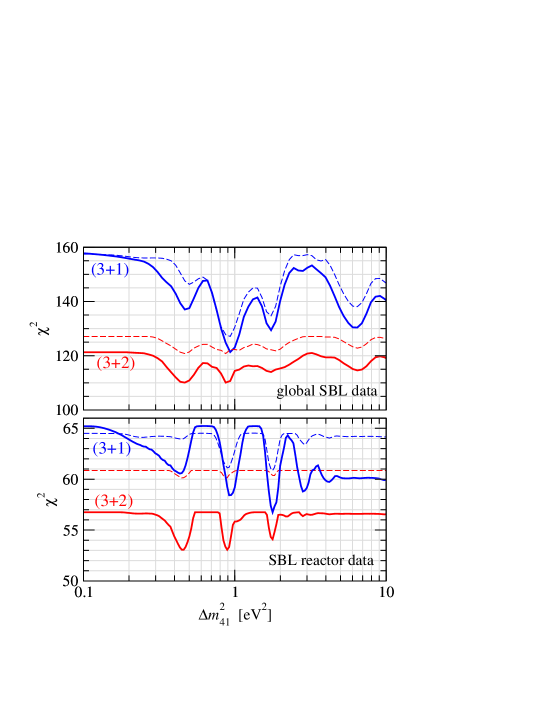
Figure 1: $\chi^{2}$ from global SBL data (upper panel) and from SBL reactor data alone (lower panel) for the 3+1 (blue) and 3+2 (red) scenarios. Dashed curves were computed using the old reactor antineutrino flux prediction [20], solid curves are for the new one [4]. All undisplayed parameters are minimized over. The total number of data points is 137 (84) for the global (reactor) analysis.

The $\chi^{2}$ of the ”3+2” model fit to the SBL oscillation data is shown in Fig. 1. It appears that there is more than one solution for the oscillation parameters. In the following, the four best fits indicated in [13] plus the best fit point of the preliminary updated analysis by Karagiorgi et al. [21] and the best fit by Giunti-Laveder [24] are considered (see Tab. 1).

	$\Delta m^{2}_{41}$	$|U_{e4}|$	$|U_{\mu 4}|$	$\Delta m^{2}_{51}$	$|U_{e5}|$	$|U_{\mu 5}|$	$\delta/\pi$	$\chi^{2}$/dof
1)	0.47	0.128	0.165	0.87	0.1380	0.148	1.64	$110.4/130$
2)	0.47	0.117	0.201	1.70	0.1150	0.101	1.39	$114.4/130$
3)	1.00	0.133	0.162	1.60	0.151	0.078	1.48	$114.4/130$
4)	0.90	0.123	0.163	6.30	0.135	0.091	1.67	$115.0/130$
5)	0.92	0.14	0.14	26.60	0.077	0.15	1.7	182.6/192
6)	0.90	0.158	0.152	1.61	0.130	0.078	1.51	91.6/100

Table 1: Parameter values and $\chi^{2}$ at the global best fit points for the four best “3+2” fit points of [13], table entries 1-4, the best fit of Karagiorgi et al. [21], entry (5); ($\Delta m^{2}$’s in eV²) and the best fit by Giunti-Laveder [24], entry (6).

3.6 Probabilities at the Far detector

The oscillation probabilities $P(\nu_{\mu}\rightarrow\nu_{e})$, $P(\nu_{e}\rightarrow\nu_{e})$ and $P(\nu_{\mu}\rightarrow\nu_{\mu})$ are computed at a distance of 850 m from the proton target for the six best values reported in Tab. 1 (see Fig. 2). Many interesting features occur within the interplay of appearance/disappearance either for $\nu_{\mu}$ or $\nu_{e}$ sectors, the most exquisite distinctiveness being that the scenario may be rather complicate. Therefore to disentangle that scenario we will need the best measurements of $\nu_{\mu}$ and $\nu_{e}$ as well as $\overline{\nu}_{\mu}$ and $\overline{\nu}_{e}$ in the widest available energy range.

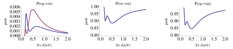
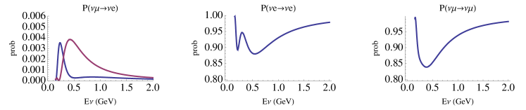
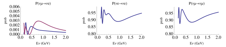
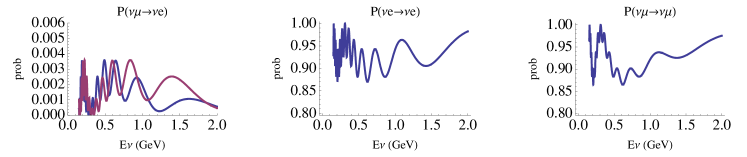
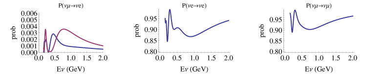
Figure 2: Oscillation probabilities computed at a baseline of 850 m for the four best fit points of “3+2”  [13], the best fit of [21] and the best fit of [24]. $P(\nu_{\mu}\rightarrow\nu_{e})$ on the left (neutrinos in blue, antineutrinos in magenta), $P(\nu_{e}\rightarrow\nu_{e})$ at center and $P(\nu_{\mu}\rightarrow\nu_{\mu})$ on the right.

In any case we like to underline some attractive outcomes from these probability computations, primarily for the “3+2” models:

• in the electron sector competition occurs between $\nu_{e}$ disappearance and $\nu_{e}$ appearance through the $\nu_{\mu}\rightarrow\nu_{e}$ transitions. This is the tricky way by which “3+2” may cancel out $\nu_{e}$ appearance in MiniBooNE.

• The different results in $\nu_{e}$ and $\overline{\nu}_{e}$ by MiniBooNE may be explained by the behavior of the $\overline{\nu}_{\mu}\rightarrow\overline{\nu}_{e}$ transitions which take into account the CP violation introduced by the “3+2” models.

• A low energy $\nu_{e}$ excess emerges. The peak is entirely due to the interference term of Eq. 2 and it would be a signature of the existence of not one, but two sterile neutrinos.
  It should be noted that the MiniBooNE low energy excess detected in the neutrino run can be accommodated by the “3+2” models. However when disappearance data are also considered the peak of the interference term does not fit anymore the measure [13].

• A sizable $\nu_{\mu}$ disappearance probability as large as 15% at the oscillation maximum is predicted below 1$\div$2 GeV, depending on the different best fits.

3.7 Neutrino Rates at the Far detector

Neutrino interaction rates are computed using the neutrino flux discussed in Sect. 4, the GENIE [25] cross sections and the above-mentioned probabilities. Event rates are normalized to 2 years’ run of the positive focussing neutrino beam, with 30 kW proton beam power, and 3 years’ run of negative focussing neutrino beam. A neutrino efficiency of 100% is considered, while energy resolution effects and systematic errors are not included in the plots.

By considering the six test points of Tab. 1 event rate spectra are displayed in Fig. 3 for $\nu_{e}$. Results without oscillations, with $\nu_{e}$ disappearance only and with both $\nu_{e}$ disappearance and appearance, generated by $\nu_{\mu}\rightarrow\nu_{e}$ transitions, are shown.

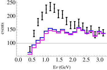
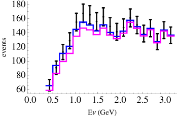
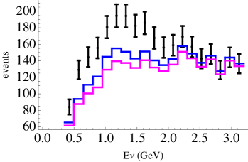
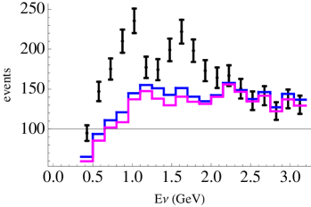
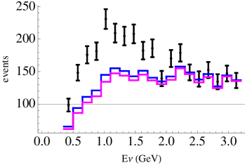
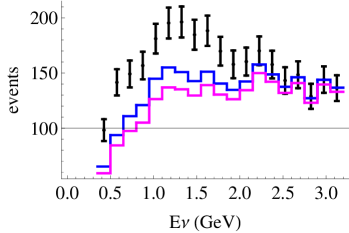
Figure 3: Electron neutrino spectra for the six test points described in the text. Blue lines corresponds to no oscillations, magenta to disappearance only, black points with statistical error bars corresponds to disappearance plus appearance events.

The number of expected $\nu_{\mu}$ events are displayed in Fig. 4, while event rates in the energy range $0.2\;GeV<E_{\nu}<2\;GeV$ are reported in Tab. 2 and Tab. 3, for $\nu_{\mu}$ and $\nu_{e}$, respectively. The integral effect is not negligible (up to 6%) and the distinctive spectral signature is clearly detectable.

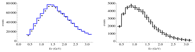
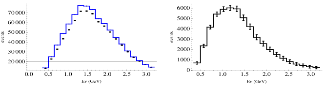
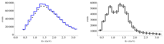
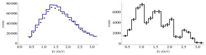
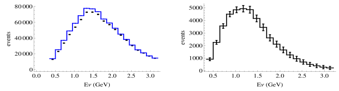
Figure 4: $\nu_{\mu}$ event rates (left) where blue lines correspond to no-oscillation and black points with statistical error bars (not visible) include disappearance. Difference between rates estimated with and without oscillation (right). The six rows refer to the test points discussed in the text.

Fit point	No-Osc.	Disappearance
1)	605792	569060
2)	605792	576102
3)	605792	560108
4)	605792	564136
5)	605792	554629
6)	605792	567584

Table 2: $\nu_{\mu}$ events computed for $0.2\;<E_{\nu}<2\;\rm{GeV}$ and two years’ run at 30 kW, for the 6 test points described in the text.

Fit point	No-Osc.	Disapp.	Disapp. + App.
1)	1424	1349	2065
2)	1424	1342	1512
3)	1424	1306	1788
4)	1424	1326	2018
5)	1424	1349	1977
6)	1424	1283	1835

Table 3: $\nu_{e}$ events with $0.3\;<E_{\nu}<2\;\rm{GeV}$ computed for two years’ run at 30 kW, for the 6 test points described in the text.

3.8 Antineutrino Rates at the Far detector

If CPT holds, data taken with antineutrino beams should provide identical $\nu_{e}$ and $\nu_{\mu}$ disappearance rates. If CP is violated, as predicted by all the “3+2” best fit points, $\overline{\nu}_{e}$ appearance rate results to be rather high and the signal could not be missed. As an example we display in Table 4 event rates as predicted by the “3+2” best fit and in Figure 5 the corresponding signal plots.

Section 7 quantitatively discusses the possibility of measuring both $\nu_{\mu}$ and $\overline{\nu}_{\mu}$ disappearance rates with the NESSiE Spectrometer in the antineutrino run.

events	No-Osc.	Disappearance	Disapp. + App.
$\nu_{e}$ (0.3-2 GeV)	1134	1078	1475
$\nu_{\mu}$ (0.3-2 GeV)	312439	290791

Table 4: Event numbers in antineutrino mode, best fit (1), 3 years’ of data taking

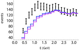
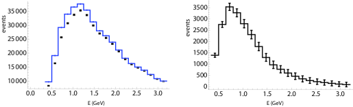
Figure 5: Left panel: $\nu_{e}$ +$\overline{\nu}_{e}$ events in the antineutrino beam, computed for the first test point of Table 1, blue line corresponds to non-oscillated events, magenta line to disappearance only and points with errors correspond to oscillated events. Central panel: $\nu_{\mu}$ +$\overline{\nu}_{\mu}$ events, blue line corresponds to non-oscillated events, points with errors (not visible) to oscillated events. Right panel: $\nu_{\mu}$ +$\overline{\nu}_{\mu}$ events are shown as expected minus measured.

3.8.1 “3+1” neutrino oscillations model

In the so called “3+1” model the flavor neutrino basis includes three active neutrinos $\nu_{e}$, $\nu_{\mu}$, $\nu_{\tau}$ and a sterile neutrino $\nu_{s}$. The effective flavor transition and survival probabilities in short-baseline (SBL) experiments are given using the standard notation by

$$\hbox{}P_{\hbox to0.0pt{\kern-2.5pt$\overset{\scriptscriptstyle(-)}{\phantom{\nu}}$\hss}{{\nu}_{\alpha}}\to\hbox to0.0pt{\kern-2.5pt$\overset{\scriptscriptstyle(-)}{\phantom{\nu}}$\hss}{{\nu}_{\beta}}}^{\text{SBL}}=\sin^{2}2\vartheta_{\alpha\beta}\sin^{2}\left(\frac{\Delta{m}^{2}_{41}L}{4E}\right)\qquad(\alpha\neq\beta)\,,$$ (5)

$$\hbox{}P_{\hbox to0.0pt{\kern-2.5pt$\overset{\scriptscriptstyle(-)}{\phantom{\nu}}$\hss}{{\nu}_{\alpha}}\to\hbox to0.0pt{\kern-2.5pt$\overset{\scriptscriptstyle(-)}{\phantom{\nu}}$\hss}{{\nu}_{\alpha}}}^{\text{SBL}}=1-\sin^{2}2\vartheta_{\alpha\alpha}\sin^{2}\left(\frac{\Delta{m}^{2}_{41}L}{4E}\right)\,,$$ (6)

for $\alpha,\beta=e,\mu,\tau,s$, with

$$\hbox{}\sin^{2}2\vartheta_{\alpha\beta}=4|U_{\alpha 4}|^{2}|U_{\beta 4}|^{2}\,,$$ (7)

$$\hbox{}\sin^{2}2\vartheta_{\alpha\alpha}=4|U_{\alpha 4}|^{2}\left(1-|U_{\alpha 4}|^{2}\right)\,.$$ (8)

The key features of this model are:

1. All effective SBL oscillation probabilities depend only on the absolute value of the largest squared-mass difference $\Delta{m}^{2}_{41}$.

2. All oscillation channels are open, each one with its own oscillation amplitude.

3. The oscillation amplitudes depend only on the absolute values of the elements in the fourth column of the mixing matrix, i.e. on three real numbers with sum less than unity, since the unitarity of the mixing matrix implies $\sum_{\alpha}|U_{\alpha 4}|^{2}=1$

4. CP violation cannot be observed in SBL oscillation experiments, even if the mixing matrix contains CP-violation phases. In other words, neutrinos and antineutrinos have the same effective SBL oscillation probabilities.

The global fit of all data in “3+1” scheme yields the best-fit values of the oscillation parameters listed in Tab. 5.

	3+1
$\chi^{2}_{\text{min}}$	$100.2$
NDF	$104$
GoF	$59\%$
$\Delta{m}^{2}_{41}\,[\text{eV}^{2}]$	$0.89$
$|U_{e4}|^{2}$	$0.025$
$|U_{\mu 4}|^{2}$	$0.023$
$\Delta\chi^{2}_{\text{PG}}$	$24.1$
$\text{NDF}_{\text{PG}}$	$2$
PGoF	$6\times 10^{-6}$

Table 5: Values of $\chi^{2}$, number of degrees of freedom (NDF), goodness-of-fit (GoF) and best-fit values of the mixing parameters obtained in 3+1 fits of short-baseline oscillation data. The last three lines give the results of the parameter goodness-of-fit test, $\Delta\chi^{2}_{\text{PG}}$, number of degrees of freedom ($\text{NDF}_{\text{PG}}$) and parameter goodness-of-fit (PGoF).

Figures 6 and 7 show the allowed regions in the $\sin^{2}2\vartheta_{e\mu}$–$\Delta{m}^{2}_{41}$, $\sin^{2}2\vartheta_{ee}$–$\Delta{m}^{2}_{41}$ and $\sin^{2}2\vartheta_{\mu\mu}$–$\Delta{m}^{2}_{41}$ planes, respectively, together with the marginal $\Delta\chi^{2}$’s for $\Delta{m}^{2}_{41}$, $\sin^{2}2\vartheta_{e\mu}$, $\sin^{2}2\vartheta_{ee}$ and $\sin^{2}2\vartheta_{\mu\mu}$.

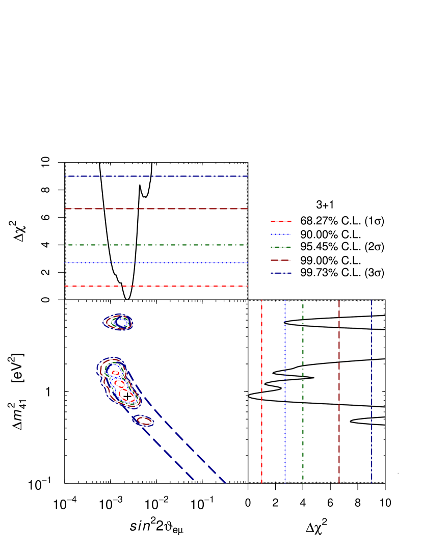
Figure 6: Allowed regions in the $\sin^{2}2\vartheta_{e\mu}$–$\Delta{m}^{2}_{41}$ plane and marginal $\Delta\chi^{2}$’s for $\sin^{2}2\vartheta_{e\mu}$ and $\Delta{m}^{2}_{41}$ obtained from the global fit of all the considered data in 3+1 schemes. The best-fit point corresponding to $\chi^{2}_{\text{min}}$ is indicated by a cross. The isolated dark-blue dash-dotted contours enclose the regions allowed at $3\sigma$ by the analysis of appearance data (the $\bar{\nu}_{\mu}\to\bar{\nu}_{e}$ data of the LSND, KARMEN and MiniBooNE experiments and the $\nu_{\mu}\to\nu_{e}$ data of the NOMAD [26] and MiniBooNE experiments).

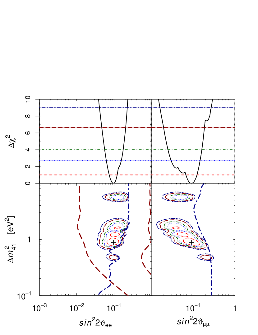
Figure 7: Allowed regions in the $\sin^{2}2\vartheta_{ee}$–$\Delta{m}^{2}_{41}$ and $\sin^{2}2\vartheta_{\mu\mu}$–$\Delta{m}^{2}_{41}$ planes and marginal $\Delta\chi^{2}$’s for $\sin^{2}2\vartheta_{ee}$ and $\sin^{2}2\vartheta_{\mu\mu}$ obtained from the global fit of all the considered data in 3+1 schemes. The best-fit point corresponding to $\chi^{2}_{\text{min}}$ is indicated by a cross. The line types and color have the same meaning as in Fig. 6. The isolated dark-blue dash-dotted lines are the $3\sigma$ exclusion curves obtained from reactor neutrino data in the left plot and from CDHS and atmospheric neutrino data in the right plot. The isolated dark-red long-dashed lines delimit the region allowed at 99% C.L. by the Gallium anomaly.

The proposed NESSiE experiment aims at exploring these regions.

3.9 3+1 and CPT violation model

The only implementation among 3+1 models able to fit global data is the 3+1 and CPT violation model of Giunti-Laveder [3, 14]. The model was inspired by the analysis of the electron neutrino data of the Gallium radioactive source experiments and the electron antineutrino data of the Bugey [22] and Chooz [23] reactor experiments in terms of neutrino oscillations allowing for a CPT-violating difference of the squared-masses and mixings of neutrinos and antineutrinos.

It was found that the discrepancy between the disappearance of electron neutrinos indicated by the data of the Gallium radioactive source experiments and the limits on the disappearance of electron antineutrinos given by the data of reactor experiments reveal a positive CPT-violating asymmetry of the effective neutrino and antineutrino mixing angles. If there is a violation of the CPT symmetry, it is possible that the effective parameters governing neutrino and antineutrino oscillations are different. From a phenomenological point of view, it is interesting to consider the neutrino and antineutrino sectors independently, especially in view of the experimental tests considered in this proposal.

The parameters of the model are reported in Tab. 6.

$\Delta m^{2}_{41}$	$|U_{e4}|$	$|U_{\mu 4}|$	$\overline{\Delta m}^{2}_{41}$	$|\overline{U}_{e4}|$	$|\overline{U}_{\mu 4}|$
1.92	0.275	0.0	0.47	0.068	0.886

Table 6: Best fit parameters of the 3+1 and CPT violation model

In this scenario, neutrinos undergo $\nu_{e}\rightarrow\nu_{e}$ transitions only, see Fig. 8, while antineutrinos have a much richer phenomenology [28, 29].

The $\nu_{e}$ spectra computed for two years’ run at 30 kW are reported in Fig. 9. According to 3+1 and CPT violation model $\nu_{e}$ disappearance should be clearly detectable 1127 events detected against a prediction of 1424 for $0.3<E_{\nu}<2$ GeV (Tab. 7).

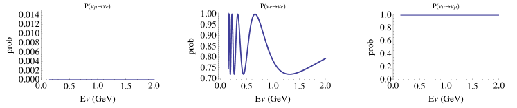
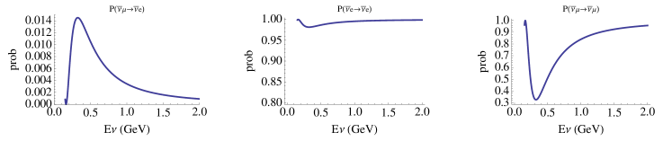
Figure 8: Oscillation probabilities computed for the 3+1 and CPT violation model. $P(\nu_{\mu}\rightarrow\nu_{\mu})$ and $P(\nu_{\mu}\rightarrow\nu_{e})$ are not displayed because they are predicted to be null by the model.

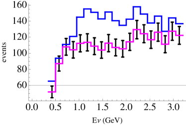
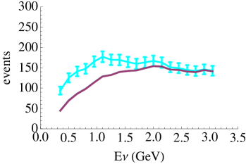
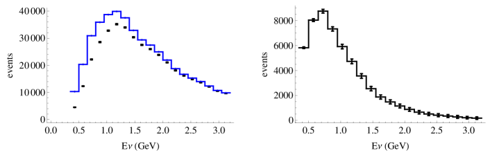
Figure 9: Top panel: $\nu_{e}$ event rates in the negative focussing beam (left) and $\overline{\nu}_{e}$ event rates in the positive focussing beam (right) computed assuming the 3+1 and CPT violation model. Non-oscillated rates are displayed as a blue histogram. Bottom panel: $\overline{\nu}_{\mu}$ event rates in the positive focussing beam: on the right absolute event rates computed with (point with errors) and without (blue histogram) oscillations following the 3+1 and CPT violation model; on the left the difference between expected and measured events is shown.

events		No-Osc.	Disapp.	Disapp. + App.
$\nu$ mode	$\nu_{e}$ (0.3-2 GeV)	1424	1127	1127
$\overline{\nu}$ mode	$\nu_{e}$ (0.3-2 GeV)	1260	1254	1699
$\overline{\nu}$ mode	$\nu_{\mu}$ (0.3-2 GeV)	329328	277335

Table 7: Events expectation for the 3+1 and CPT violation model

4 The Neutrino Beam

The NESSiE detector is planned for exposure to the CERN-PS neutrino beam-line, originally used by the BEBC/PS180 collaboration [30] and re-considered later by the I216/P311 [31] proposal. The baseline setup used by BEBC/PS180 consisted in a 80 cm long, 6 mm diameter beryllium-oxide target followed by a single pulsed magnetic horn operated at 120 kA. The PS can deliver 3 $\cdot$ 10¹³ protons per cycle at 19.2 GeV kinetic energy in the form of 8 bunches of about 60 ns in a window of 2.1 $\mu s$, integrating about 1.25 $\cdot$ 10²⁰ protons on target (p.o.t.)/year under reasonable assumptions. The existing decay tunnel, which has a cross section of 3.5 $\times$ 2.8 m² for the first 25 m of length and 5.0 $\times$ 2.8 m² for the remaining 20 m, is followed by a 4 m thick iron shield and 65 m of earth. With respect to the original configuration, the target and the horn must be redesigned and reconstructed due to the present level of radioactivity while the proton beam line magnets and supplies could be recovered (see Sect. 4.3).

4.1 Beam simulation

The BEBC/PS180 fluxes were reproduced by I216/P311 in their Letter of Intent [32] using a simulation based on GEANT3 and GFLUKA. The comparison was updated using a simulation adapted from the one used for the CNGS beam for their proposal [31]. For this memorandum a GEANT4 and FLUKA [33] based simulation has been developed to profit of a modern programming framework and to investigate possible improvements in the beam performance.

The generation of proton-target interactions is done with FLUKA-2008 while GEANT4 is used for tracking in the magnetic field and the materials and for the treatment of meson decays. The simulation program, thoroughly described in [34], has been modified to take finite-distance effects into account, which are particularly important due to the short baselines involved (127 and 885 $m$ measured from the target to the beginning of the LAr detector). Neutrinos crossing the LAr and Spectrometer volumes are directly scored using a full simulation avoiding any weighting approach. A sample of $10^{7}$ simulated p.o.t. was produced and has been used in the following.

In order to benchmark the GEANT4 simulation the existing setup used for the BEBC/PS180 experiment has been reproduced [35]. The layout of the considered volumes is shown in Fig. 10.

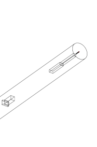
Figure 10: Layout of the focussing system and Near detector station in the GEANT4 simulation.

The spectrum shape of the $\nu_{\mu}$ is in good agreement with that calculated by the I216/P311 experiment whereas the obtained normalization is instead 27% lower (Fig. 11). Investigations are ongoing to understand this difference, in particular the implementation of the geometry and the hadro-production models are under checking. The flux reduction resulting from negative-focussing, which amounts to about 40%, is well reproduced.

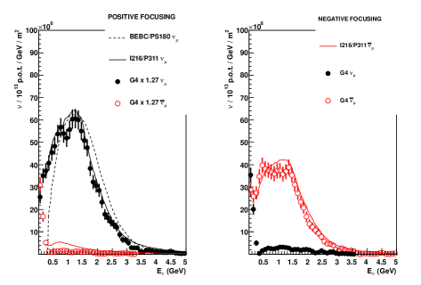
Figure 11: Comparison of the present simulation (dots) with those of BEBC (dashed line) and I216/P311 (continuous line) for positive-focussing mode (left) and negative-focussing mode (right). G4 stands for the new simulation obtained with GEANT4 which introduces a 1.27 reduction factor with respect to the old simulation. Fluxes are referred a distance of 825 $m$ from the target (BEBC site). The target starts at 35 $cm$ upstream of the BEBC/PS180 horn, which is operated at 120 kA.

Neutrino fluxes at the Far and Near Spectrometers in positive and negative-focussing are shown in Fig. 12. Accounting for the Spectrometer geometries and locations we obtain a ratio $\nu$/p.o.t. of about $10^{-2}$ in the Near station and a further reduction of a factor of about 20 in the Far location. The fractions of ($\nu_{\mu}$, $\bar{\nu}_{\mu}$, $\nu_{e}$, $\bar{\nu}_{e}$) in the Near Spectrometer are (92.3, 6.6, 0.87, 0.26)% in positive-focussing mode and (12.2, 86.6, 0.49, 0.75)% in negative-focussing mode. In the Far detector numbers are very close to the previous ones. The electron neutrino contamination is in agreeement with the estimates of I216/P311.

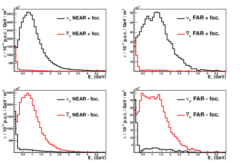
Figure 12: $\nu_{\mu}$ fluxes (black) and $\bar{\nu}_{\mu}$ fluxes (red) at the Near (left column) and Far (right column) Spectrometers in positive-focussing (upper row) and negative-focussing (lower row) modes.

The energy dependence of the electron and wrong-sign muon contamination is shown in Fig. 13. It can be noticed that the $\nu_{e}$ contamination in the energy region between 500 $MeV$ and 1 $GeV$ is very low, approaching a minimum of 0.4%, to the benefit of the $\nu_{e}$ appearance search. The contamination of $\bar{\nu}_{\mu}$ in the $\nu_{\mu}$ beam is quite significant especially at high energy where the spectrometer charge separation becomes thus very important.

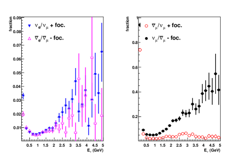
Figure 13: Left: $\nu_{e}/\nu_{\mu}$ ratio in positive-focussing mode and $\bar{\nu}_{e}/\bar{\nu}_{\mu}$ ratio in negative-focussing mode in the Near Spectrometer as a function of the neutrino energy. Right: $\bar{\nu}_{\mu}/\nu_{\mu}$ ratio in positive-focussing mode and $\nu_{\mu}/\bar{\nu}_{\mu}$ ratio in negative-focussing mode in the Near Spectrometer as a function of the neutrino energy.

In particular, after folding the spectrum with the CC cross section (Fig. 14), one can see that the negative-focussing beam at high energy yields a comparable mixture of $\mu^{-}$ and $\mu^{+}$. The Spectrometer charge separation allows studying the behavior of both CP states at the same time.

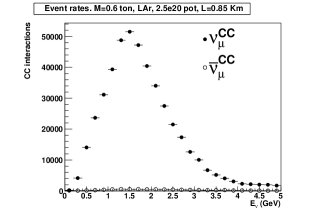
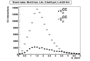
Figure 14: Comparison of $\nu_{\mu}^{CC}$ and $\bar{\nu}_{\mu}^{CC}$ event rates for the positive (left) and negative-focussing (right) beams.

The distribution of the impact points of the $\nu_{\mu}$ in the Near Spectrometer is shown in the upper left plot of Fig. 15. The center of the beam is displaced in the bottom direction of 1 m and the radial beam profile can be well fitted with a Gaussian having a $\sigma$ of about 4 m (Fig. 15 upper right and lower left plots)

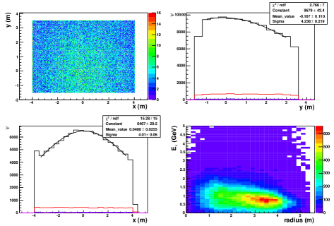
Figure 15: Up left. Distribution of the neutrino impact points in the transverse plane, $X$ vs $Y$. Up right: $X$ projection. Bottom left: $Y$ projection. The black histogram represents the $\nu_{\mu}$, the red histogram the $\bar{\nu}_{\mu}$. Bottom right: $E_{\nu_{\mu}}$ vs $\sqrt{X^{2}+Y^{2}}$. Results refer to positive-focussing mode.

The spectrum of $\nu_{\mu}$ at the Near detector peaks at lower energies due to the fact that many interacting neutrinos are off-axis and then tend to have a lower mean energy (Fig 16, left). Nevertheless, restricting to the central region, i.e. the region that subtends an angle similar to that of the Far detector, the shapes tend to get closer. This selection allows smaller corrections in the Near/Far ratio thus decreasing the systematics. The correlation between the energy and the radius of the neutrino impact point is shown the lower right plot of Fig. 15. The shape of the $\nu_{e}$ spectrum on the other hand is more similar in the Near and Far locations (Fig 16, right) due to the predominantly 3-body decay origin.

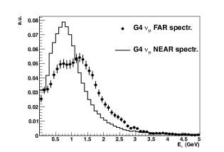
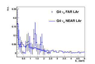
Figure 16: Comparison of the $\nu_{\mu}$ (left) and $\nu_{e}$ (right) fluxes in the Near and Far LAr detector in positive-focussing mode. G4 stands for the new simulation obtained with GEANT4 which introduces a 1.27 reduction factor with respect to the old simulation.

4.2 New horn designs

By keeping the basic geometry of the beam (size of the target and horn hall, decay tunnel, shielding) unchanged, studies of several modified horns and targets in addition to the BEBC original setup are undergoing, an optimized design of new and possibly improved beam optics being pursued. Our aim is to move towards a high intensity $\nu_{\mu}$ flux in order to reduce the statistical errors, peaking at $\langle E_{\nu_{\mu}}\rangle\sim$ 1 GeV to match the $\Delta m^{2}\sim 1$ eV² region. For the reduction of systematics in the $\nu_{\mu}\to\nu_{e}$ appearance channel the high energy tail above $\sim$ 2.5 GeV should be reduced to suppress $\pi^{0}$ production and the intrinsic $\nu_{e}$ contamination should be kept small.

Preliminary studies performed with bi-parabolic horns à la NuMI [36] indicate room for improvement. In particular in the last decades the feasibility of horns pulsed at high currents of order 300 kA has been demonstrated. The fluxes obtained with a new bi-parabolic horn pulsed at 246 kA, are shown in Fig. 17. An overall flux gain is obtained, particularly at low energy. This would be particularly useful to extend the sensitivity towards smaller $\Delta m^{2}$.

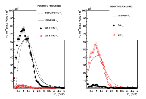
Figure 17: New horn fluxes compared to BEBC and I216/P311. The meaning of the symbols is as in Fig. 11, in particular G4 stands for the new simulation obtained with GEANT4 which introduces a 1.27 reduction factor with respect to the old simulation.

Since the interval of the interesting $\Delta m^{2}$ regions is large it would be desirable to get a configuration capable of scanning different neutrino energy regions thus adapting to the physics indications coming from the data taking. Despite the fact that the overall features of the neutrino beam are dictated by the proton energy, an effective way for varying the mean energy consists in using a tunable target-horn distance.

While keeping the shape of the original horn unchanged, a scan in the scatter plane (current ($i$) vs target longitudinal position ($z_{targ}$)) was performed to study the effects of the fluxes in terms of $\nu_{\mu}$ normalization, energy distribution and contaminations. Results are shown in Fig. 18 for positive-focussing at the Far location. Plots show how the integral $\nu_{\mu}$ flux is increased going to higher currents; pushing the target upstream (downstream) corresponds to decrease (increase) the $\bar{\nu}_{\mu}$ contamination and to probe the high(low)-energy region. Two configurations yielding very different spectra are shown in Fig. 19. It is interesting to notice that these fluxes are obtained using the same current of 300 kA just varying the position for the target.

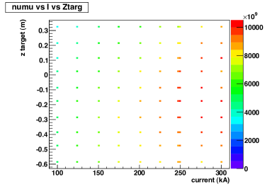
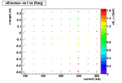
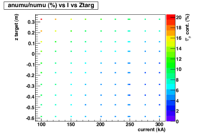
Figure 18: Dependence of the integral $\nu_{\mu}$ flux (top), the $\nu_{\mu}$ mean energy (middle) and the $\bar{\nu_{\mu}}$ contamination (bottom) from ($I$, $z_{targ}$) with a test bi-parabolic horn. Results are shown for positive-focussing at the Far location.

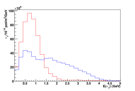
Figure 19: Two extreme low (red) and high-energy (blue) configuration fluxes arising from the scan in the ($I$, $z_{targ}$) plane. The current is 300 kA and the position of the beginning of the target with respect to the beginning of the horn is +32 and -58 cm respectively. The fluxes refer to a distance of 825 m.

4.3 Beam reactivation

Preliminary evaluations for a renovated TT7 PS neutrino beam line have been already completed at CERN [37]. The TT7 transfer line, the target chamber and the decay tunnel are in good shape and available for the installation of the proton beam line, target and magnetic horn. The main dipoles, quadrupoles, correction dipoles and possibly the transformer for the magnetic horn can be recuperated, reducing significantly the cost and time schedule. The target and secondary beam focussing design can profit of the CNGS experience as well as monitoring systems, primary beam steering and target alignment [38].

The study dating back to 1999 [31] estimated the time required to be approximately 2 years for a total cost of about 4.2 MSF detailed as follows:

• power converters of TT1 and TT7 magnets: consolidation and lower level electronics (1.1 MSF);

• civil engineering, mostly new housing for converters (0.5 MSF);

• removal of 400 m³ radioactive waste material in TT7, provisions and installations for radiation protections, access control ($<$ 0.5 MSF);

• beam line installation, vacuum chamber, general mechanics (0.4 MSF);

• beam monitoring instrumentation (0.4 MSF);

• new target and horn (0.4 MSF);

• new pillars and platform in the Near experimental hall (50 KSF).

5 Spectrometer Design Studies

The main purpose of a spectrometer placed downstream of the target section is to provide charge and momentum reconstruction of muons escaping from LAr detection. This choice would provide a double benefit with respect to a LAr detector running in stand-alone mode. Firstly a precise muon momentum reconstruction would allow a good kinematical closure of CC events occurred in LAr in particular in the high energy tail where the muon momentum resolution is poorer. Secondly muon charge separation would allow us to disentangle $\nu_{\mu}$ and $\bar{\nu}_{\mu}$ disappearance channels in particular in the negative-focussing option where wrong-sign contamination is larger. This would allow tackling CP and CPT violating scenarios in an unambiguous way.

In addition, a proper mass-granularity combination would allow a coarse reconstruction of $\nu_{\mu}^{CC}$ events occurring within the Spectrometer itself and provide a way to use the Spectrometer in stand-alone mode, too.

We characterize the detector by evaluating the physics performances in terms of CC disappearance and the sensitiveness to ($\Delta m^{2},\sin^{2}2\theta$) values predicted by the models described in Sect. 3. We recall that with a suitable detector the old CDHS $\nu_{\mu}$ disappearance limit will be tested in just one day of data taking.

Moreover we assumed some “a priori” constraints by defining a realistic, conservative, relatively inexpensive apparatus.

5.1 Magnetic field in Iron

A magnetized iron spectrometer was chosen as baseline option. Its design was such to match the required sensitivity of the experiment with respect to the sterile neutrino models of Sect. 3. The basic parameters to be tuned are the transverse width, the longitudinal dimensions, the iron slab thickness and the tracking detector resolution. The transverse and longitudinal dimensions constrain the detector acceptance and hence the detectable number of events which are directly related to the $|U_{\mu 4}|$ and $|\overline{U}_{\mu 4}|$ mixing parameters (see in particular Table 1 of Sect. 3). On the other hand the target segmentation sets bounds on muon momentum and charge reconstruction and are directly related to $\Delta m^{2}_{41}$ and $\overline{\Delta m}^{2}_{41}$.

The transverse width has to be large enough in order to maximize the detection of muons escaping from LAr. Monte Carlo simulation has shown that a transverse size matching the LAr acceptance ($\sim 8\times 5$ m² in the Far site (FD) provides a good performance while still keeping the detector size at a feasible level (doubling the dimensions would improve the sensitivity to $|U_{\mu 4}|$ by 5%).

Fig. 20 shows the muon impact point distribution along the $x$ axis at FD.

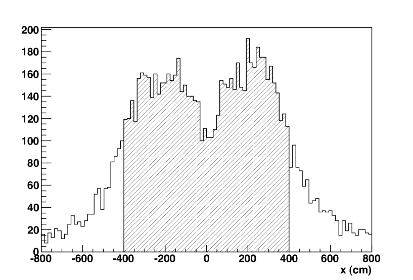
Figure 20: Distribution of muon impact points along the $x$ axis, at the Far site (FD). The dip at the center of the distribution and the sharp tails on the sides are due to the convolution with the LAr detector acceptance. The shaded area corresponds to the 78% of the total one.

Due to the relatively low energy spectrum of the PS neutrino beam the Spectrometer longitudinal size has to be large enough in order to allow energy measurement by range in a wide energy interval (see later on in this Section). Simulations have shown that 2 m of Iron contain $\sim$90% of muons in positive-focussing ($\sim$85% in negative-focussing). 5 cm thick iron slabs would allow a spectrum bin size of $\sim$60$\div$100 MeV/$\sqrt{12}\simeq 20\div 30$ MeV for perpendicularly impinging muons. Momentum reconstruction for passing-through muons ($E_{\mu}>3$ GeV/c) can be performed exploiting the track bending in the magnetic field. A detector resolution of $\sim$1 cm provides a $\sigma_{p}/p$ resolution ranging from 20% at 3 GeV/c up to 30% at 10 GeV/c (see Fig. 21).

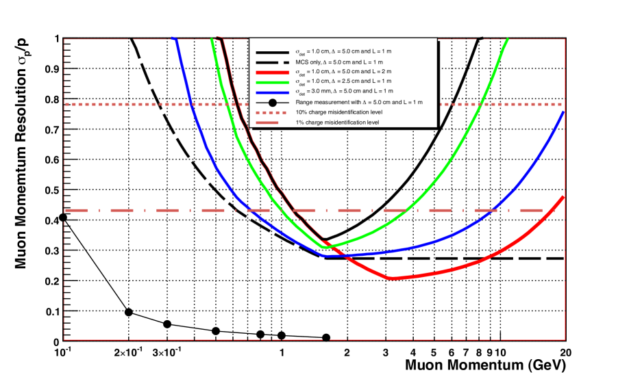
Figure 21: Muon momentum resolution as calculated for several Spectrometer configurations, with a magnetic field $B=1.5\ T$.

Muon charge assignment is performed measuring the direction of track curvature. The experimental sensitivity to $\Delta m^{2}$ scales linearly with the neutrino energy, $E_{\nu}$, and only with $\sqrt[4]{N_{events}}$. Therefore the possibility to explore CPT-violating $\nu_{\mu}$ disappearance at $\Delta m^{2}$ values below $\sim$1 eV² in a baseline of $\sim 850$ m relies on the capability to identify the muon charge with good accuracy down to $E_{\nu}$ of about few hundreds of MeV and even lower if we consider the muon residual energy reaching the Spectrometer (see Fig. 22). However in this momentum region one has to cope with the severe limits imposed by Multiple Scattering in iron which completely dominates the charge identification capability.

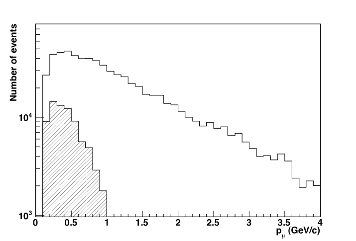
Figure 22: Energy spectrum of $\mu^{+}$ intercepted by the Spectrometer in the FD in negative-focussing for 3.75 p.o.t. The shaded region is the subsample of muons from events such that 1.27 $\times$ 1 eV${}^{2}\times L/E_{\bar{\nu}}>\pi/2$.

Since for stopping muons the path-length $L$ in the $B\cdot L$ product is fixed by range $B$ has to be as large as possible ($B\simeq 1.5$ T in iron). Once the magnetic field is fixed the momentum resolution $\sigma_{p}/p$ and the charge mis-identification $\eta$ (defined as the fraction of muon tracks whose charge is wrongly assigned) are limited at low energies by Multiple Coulomb Scattering (MCS). In order to understand qualitatively this behavior let us define $\eta$ as the fraction of muon tracks whose charge is wrongly assigned. $\eta$ is related - in the Gaussian approximation of the Moliere distribution- to the momentum resolution by

$$\eta=\frac{1}{2}\textrm{erfc}\left[{\frac{1}{\sqrt{2}(\sigma_{p}/p)}}\right]$$ (9)

where erfc is the complementary error function. The capability to separate charge-conjugated oscillation patterns depends on the available statistics and on the value of $\eta$: the lower the number of events the lower $\eta$ has to be in order to assess a separation at a given significance level. For instance neglecting systematic and statistical uncertainties on $\eta$ a $\nu/\bar{\nu}$ separation at 10% level would require $\eta\simeq 30\%$ in energy bins with 10000 events and $\eta\simeq 5\%$ with 1000 events.

The momentum resolution (or equivalently $\eta$) is the combination of two terms, the first one related to MCS and the other to measurement errors:

$$\frac{\sigma_{p}}{p}=\sqrt{\left(\frac{\sigma_{p}}{p}\right)_{MCS}^{2}+\left(\frac{\sigma_{p}}{p}\right)_{res}^{2}}$$ (10)

The two terms can be calculated e.g. for the case of uniform detector spacing as in [39, 40, 41]. The first term is almost independent of the number of measurement points along the trajectory and it is expressed as

$$\left(\frac{\sigma_{p}}{p}\right)_{MCS}\simeq 27\%\left(\frac{1.5\textrm{T}}{B}\right)\left(\frac{1\textrm{m}}{L}\right)^{1/2}$$ (11)

where L is the muon path-length in iron and is actually limited by the muon range and the spectrometer size at low and high momenta respectively. This term sets the lower irreducible limit that can be obtained by a measurement of this kind (note that $\eta\simeq 5\%$ roughly corresponds to $\sigma_{p}/p\simeq 50\%$).

The second term depends on the detector resolution and on the number of measurements (or equivalently on the iron slab thickness, $\Delta$) and, in principle, can be decreased by changing the detector sampling and/or space resolution. In this case, for $L>>5\Delta$,

$$\left(\frac{\sigma_{p}}{p}\right)_{res}\simeq 13\%\left(\frac{p}{1\textrm{GeV/c}}\right)\left(\frac{\Delta}{5\textrm{cm}}\right)^{1/2}\left(\frac{1\textrm{m}}{L}\right)^{5/2}\left(\frac{1.5\textrm{T}}{B}\right)\left(\frac{\sigma_{det}}{1\textrm{cm}}\right)$$ (12)

with the same considerations on $L$ as for equation 11.

Curves reported in Fig. 21 and Fig. 23 show the momentum resolution and the $\eta$ dependence on the muon momentum for various choices of $\Delta$ and $\sigma_{det}$ (for orthogonally impinging muons). It is apparent that at best a mis-identification $\eta$ below 5% can be obtained only for muons with momenta above $\simeq$ 500 MeV/c.

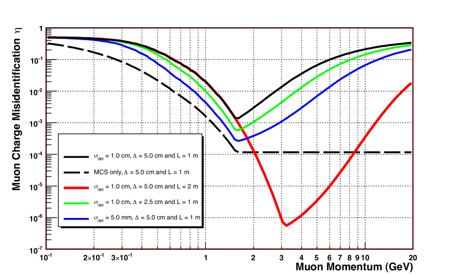
Figure 23: Muon charge mis-identification $\eta$ as calculated for several Spectrometer configurations, with a magnetic field $B=1.5\ T$.

An option to improve charge identification capability below 500 MeV is to equip the Spectrometer with a magnetic field in air just in front of the first iron slab. This possibility is discussed in the next Section.

From now on we will assume as baseline option for the FD site a dipolar magnetic Spectrometer made of two arms separated by 1 $m$ air gap. Each arm consists of 21 iron slabs 585$\times$875 cm² wide and 5 cm thick interleaved with 2 cm gaps hosting 20 Resistive Plate Chambers (RPC) detectors with $\sim$1 cm tracking resolution. The Near detector (ND) Spectrometer is a downsized replica of the FD one, the only difference being in fact the transverse dimensions (351.5$\times$625 cm²).

A calculation of the magnetic field map was performed with the COMSOL code [42]. Fig. 24 shows the distribution of the magnetic field in the 21+21 iron layers (for convenience we show in the figure the entire magnetic system, i.e. in iron and in air, the latter to be discussed later on in the Section). The fringe field is $70\div 100\leavevmode\nobreak\ G$ at $10\leavevmode\nobreak\ cm$ distance from the iron slab edge (Fig. 25).

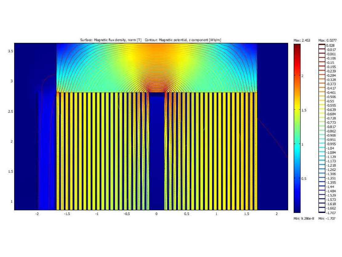
Figure 24: Simulated magnetic field distribution in the Iron Spectrometer (yellow regions) and in the air volume (light blue region on the left side, see Sect. 5.2). The horizontal axis is in meters; the color bar is in Tesla. The iron field is generated by two coils wrapped around the top and bottom iron flux return (only the upper coil is shown in the figure).

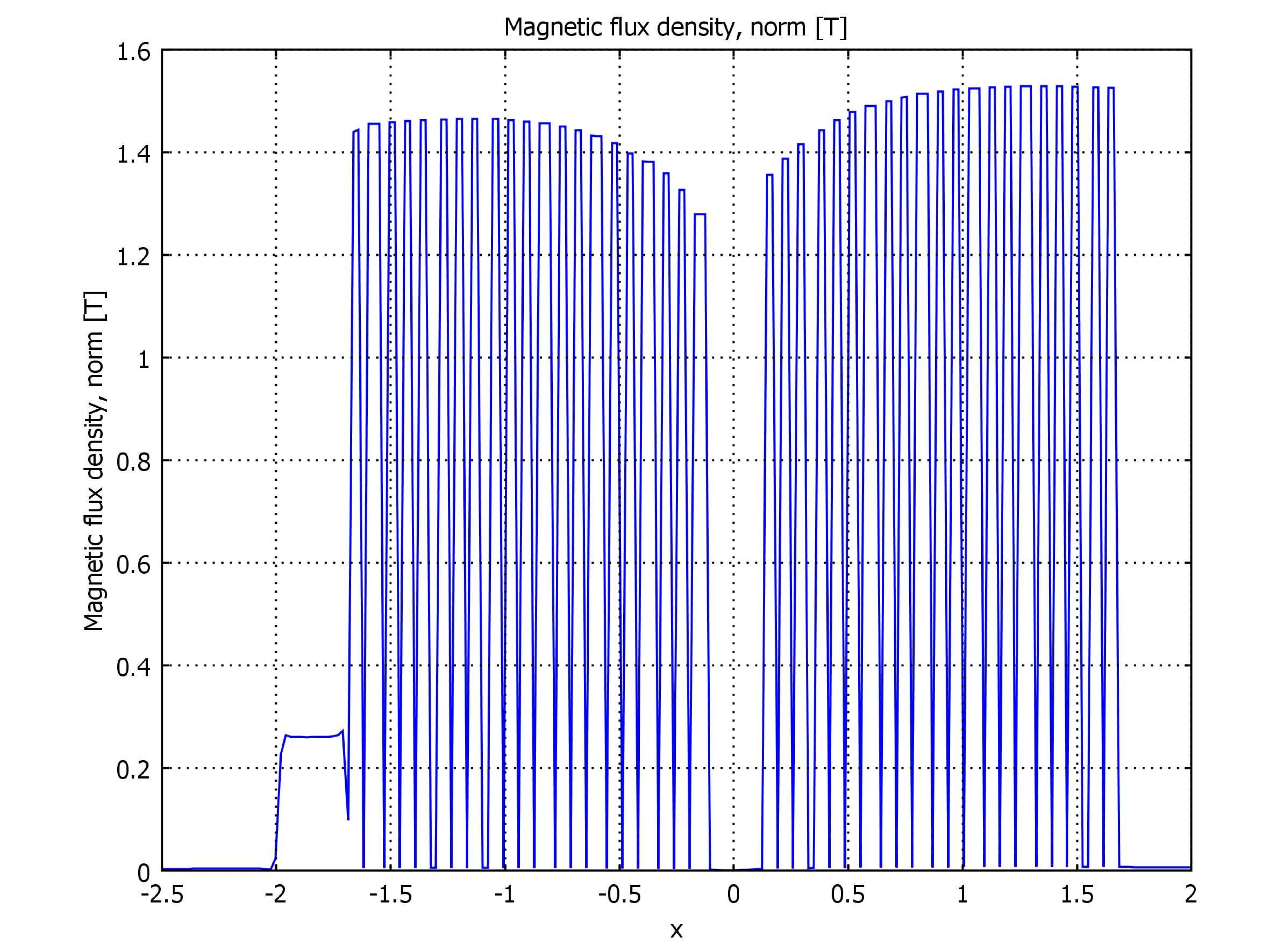
Figure 25: Magnetic field distribution in the 21+21 iron slabs and in the air volume upstream of the first iron slab. The vertical axis indicates the magnetic field in Tesla.

The simulation was performed assuming two symmetric coils wrapped around the top and bottom flux return path (following the same concept applied in the OPERA magnet [45]). The turns (36) are made of aluminum bars $27\times 19\leavevmode\nobreak\ mm^{2}$ with inner water cooling. The current density is $3\leavevmode\nobreak\ A/mm^{2}$ for a total current of $1255\leavevmode\nobreak\ A$. The total resistance is $39\leavevmode\nobreak\ mOhm$ per coil, the voltage is $49\leavevmode\nobreak\ V$ and the power $61\leavevmode\nobreak\ kW$. The conductor cross section can be increased to reduce the power dissipation.

5.2 Magnetic field in Air

For low momentum muons the effect of Multiple Scattering in iron is comparable to the magnetic bending and therefore the charge mis-identification increases (see Fig.  23) For muon momenta $<1\ GeV/c$ the charge measurement can be performed by means of a magnetic field in air. In Fig. 26 the displacement expected in the bending plane is shown for muons crossing a magnetized air volume of $30\ cm$ depth. A uniform magnetic field oriented along the $y$ axis (the bending plane is the $z,x$ one) is assumed. In the left plot the shift is shown as a function of the muon momentum for some values of the magnetic field in the $0.1-0.4$ $T$ range. In the right panel the spatial displacement in the bending plane estimated for muons of $0.5\ GeV$ in a magnetic field of $0.3\ T$ as a function of the incoming angles is plotted.

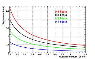
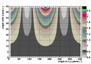
Figure 26: Left: Spatial displacement of muon trajectory in the bending plane as a function of their momentum after crossing an air magnetic field volume of $30\ cm$ thickness. Different field values in the 0.1-0.4 T range are considered. The incoming muon direction is perpendicular to the detector planes. Right: the displacement of $0.5\ GeV$ muon tracks in the $x,z$ view ($B=0.3\ T$) as a function of the initial muon angle (the color bar scale is in $cm$).

A simulation of the magnetic field in air was realized based on a coil wound on a large conductor ($54\leavevmode\nobreak\ mm\times\leavevmode\nobreak\ 19\leavevmode\nobreak\ mm$) with 170 turns distributed along the spectrometer height. A uniform magnetic field of $0.25\leavevmode\nobreak\ T$ along the $y$ axis is obtained with a coil current density of $8\leavevmode\nobreak\ A/mm^{2}$ (Fig. 24, $7000\leavevmode\nobreak\ A$ current). The fringe field at $10\leavevmode\nobreak\ cm$ distance from the edge (Fig 27) is $70\div 200\leavevmode\nobreak\ G$. The total resistance is $0.1\leavevmode\nobreak\ \Omega$, the voltage is $700\leavevmode\nobreak\ V$ and the power $4.9\leavevmode\nobreak\ MW$. This set of parameters shall be intended as preliminary and needs to be optimized for reducing the electrical power and for splitting the single large coil into a number of smaller (in height) and more manageable coils.

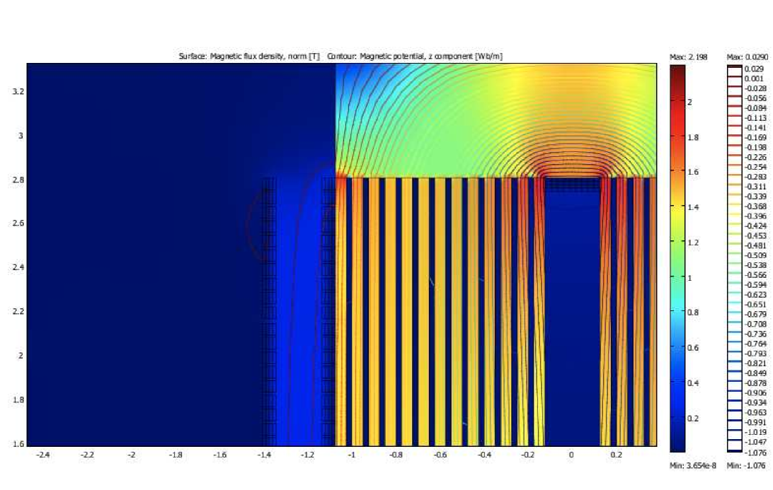
Figure 27: Simulated magnetic field distribution in the Iron Spectrometer (yellow regions) and in the air volume (light blue region on the left side). The horizontal axis is in meters. The color bar scale is in Tesla. The vertical pairs of coils used to generate the field in air are shown (on the left of the picture).

As discussed in Sec. 11 charge measurement for low momentum muons can be performed by designing a precision tracker detector of $\sim 1\ mm$ spatial resolution installed in the $z,x$ plane. The reconstruction in the $z,y$ view would be not required since the momentum could be measured by the muon range in the Iron Spectrometer.

6 Monte Carlo Detector Simulation and Reconstruction

The present proposal has been extensively developed using full-detail programming and up-to-date packages to obtain precise understanding of acceptances, resolutions and physics output. Although not all possible options have been studied, a rather exhaustive list of different magnet configurations and detector designs has been adopted as benchmark for further studies once the detector structure will be finalized.

6.1 Simulation

The aim of the simulation of the apparatus is to help the design studies reported here to understand the main features of the proposed experiment. The simulated detector consists of a ND and FD part, both made of an Liquid Argon target followed by a magnetic Spectrometer. The relative position and the dimensions of the LAr target have been kept fixed with respect to the Spectrometer for all the studies described below.

Muon neutrino and antineutrino fluxes for positive and negative beam polarity were assumed as those reported in the LAr proposal [1] since the beam analysis was still in progress. In the simulation the beam has 1 $mrad$ tilt with respect to the horizontal. For the time being no angular dependence of the neutrino fluxes has been considered. For the future we plan to take profit of the full simulation of the secondary beam line reported in the previous Sect. 4 in order to improve the simulation of the neutrino beam at both the Near and Far detector positions.

Neutrino interactions are generated in the Argon target using GENIE [25] with standard parameters and including all interaction processes (QEL, RES, DIS, NC). In additions, neutrino interactions have been generated in iron to explore the capability of the Spectrometer to reconstruct self-contained events taking advantage of its additional mass.

The propagation in the detector is implemented with either GEANT3 or FLUKA and the geometry of the detectors is described using the ROOT geometry package. The main features of the geometry implemented in the simulation are briefly described below.

The ND LAr target has dimensions $352.8\times 362.5\times 910$ $cm^{3}$ and a total mass of 162 $t$. The target is surrounded by about 1 $m$ thick light material standing for the dead material of the cryostat. The basic Spectrometer is an instrumented dipolar magnet made of two magnetized iron walls producing a field of 1.5 T intensity in the tracking region; field lines are vertical and have opposite directions in the two walls whereas track bending occurs on the horizontal plane. The thickness of the iron planes is at present envisaged to be 5 cm. Planes of bakelite RPC’s are interleaved with the iron slabs of each wall to measure the range of stopping particles and to track penetrating muons. The Spectrometer is equipped with 20 planes of 3 rows, each consisting of 2 RPC’s. At present, additional high precision Drift Tube detectors are not simulated.

The FD target consists of 2 LAr volumes each with dimensions $352.8\times 362.5\times 1820$ $cm^{3}$. The total LAr mass is 648 $t$. The FD Spectrometer is assumed to be similar to the one for the ND (20 planes each with 5 rows and 3 columns of RPC’s).

The response of the Liquid Argon detector has been sketched by sampling the position of the charged particle with 0.5 cm resolution. For the RPC’s we assume digital read-out using 2.5 $cm$ strip width and a position resolution of about 1 $cm$.

6.2 Reconstruction

A framework based on standard tools (ROOT, C++) has been developed for the reconstruction in both the Near and Far detectors.

The reference frame is defined to have the Z-axis along the beam direction, Y perpendicular to the floor pointing upwards and X completing a right-handed frame. Event reconstruction is performed separately in the two projected views XZ (bending plane) and YZ (vertical plane).

A simple track model is adopted to describe the shape of the trajectory of tracks travelling through the detector. The model is based on the standard choice of parameters used in forward geometry (i.e. intercepts, slopes, particle momentum, particle charge, … ). The reconstruction strategy is optimized to follow a single long track (the muon escaping from the neutrino-interaction region) along the Z-axis.

The reconstruction is performed in the usual two steps: Pattern Recognition (Track finding) and Track Fitting.

The task of the Pattern Recognition is to group hits into tracks. Taking into account that most of neutrino interactions generated in the LAr target have just one track reaching the Spectrometer (the muon) and assuming a read-out capable of avoiding event overlap, we postponed the development of a dedicated algorithm For the time being all the hits of the events are associated to a single track.

The Track Fitting has to compute the best possible estimate of the track parameters according to the track model. A parabolic fit is performed in the XZ plane (bending) whereas a linear fit is used for YZ plane (vertical). Particle charge and momentum are determined from the track sagitta measured in the bending plane; the track fit is corrected for material interactions (Multiple Scattering and energy loss). Each spectrometer arm provides an independent measurement of charge/momentum. A better estimation of momentum is obtained by range for muons stopping inside the Spectrometer. The implementation of a track fitting algorithm based on a Kalman filter is eventually foreseen.

7 Physics performances

In this section we address the physics performance of the FD and ND Spectrometers with and without the B field in air option.

We studied the performance of the Spectrometer using the Monte Carlo simulation detailed in the previous section. In particular we report on the negative-focussing option which is the most promising for our purposes. We have generated $10^{6}$ $\nu_{\mu}$ (NC+CC) events and $10^{6}$ $\bar{\nu}_{\mu}$ (NC+CC) events according to spectra shown in the right panel of Fig. 14. Neutrino vertices were generated within the LAr volume and each outgoing particle from the vertex was propagated in the LAr $+$ Spectrometer geometry. Each event was classified into one of the following category:

1. Fully contained events. These are events in which the neutrino vertex is contained the LAr fiducial volume and the muon track stops in the LAr fiducial volume. We considered events with a muon track escaping from the vertex at least 20 cm long.

2. Partially contained in LAr not reaching the Spectrometer. These are events with the neutrino vertex within the LAr fiducial volume and the muon track which escapes from the LAr fiducial volume which do not intercept the Spectrometer. In this case we require a muon track at least 200 cm long in order to reconstruct the muon momentum with a good momentum resolution by MCS in LAr.

3. Partially contained in LAr reaching the Spectrometer. These are events with the neutrino vertex within the LAr fiducial volume and the muon track which escapes from the LAr fiducial volume which do intercept the Spectrometer. In this case we accept also muon track shorter than 200 cm in LAr since the muon momentum information are recovered with the Spectrometer.

The last sample is further subdivided into events with a muons stopping in the Spectrometer and events passing through the whole Spectrometer (or escaping from the side). In the first case the muon momentum is reconstructed by range, in the second case by magnetic bending. The muon charge sign is always reconstructed by magnetic bending, in the air field or in the magnetized iron according to the muon energy.

Figg. 28 and  29 report the fraction of each event topology in the negative-focussing option in the Near and Far detector, respectively.

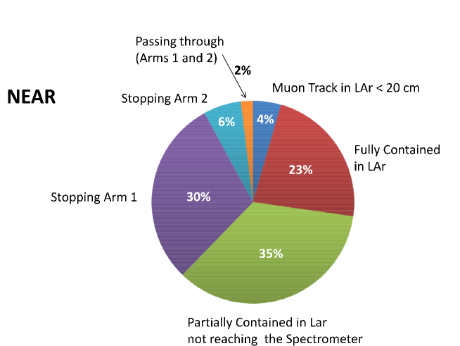
Figure 28: Fraction of events collected at the Near site by the LAr and the Spectrometer detetctors. The different topologies are detailed in the text.

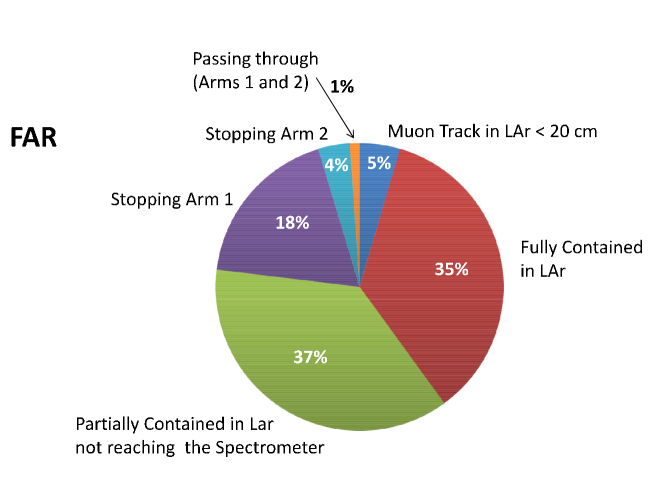
Figure 29: Fraction of events collected at the Near site by the LAr and the Spectrometer deetctors. The different topologies are detailed in the text.

In Fig. 30 we show the Spectrometer performance in terms of momentum reconstruction. In the figure the separate contributions of stopping muon, passing through going muons and low energy muons are displayed. The total muon momentum at the neutrino vertex is computed adding the contribution of the energy lost in LAr.

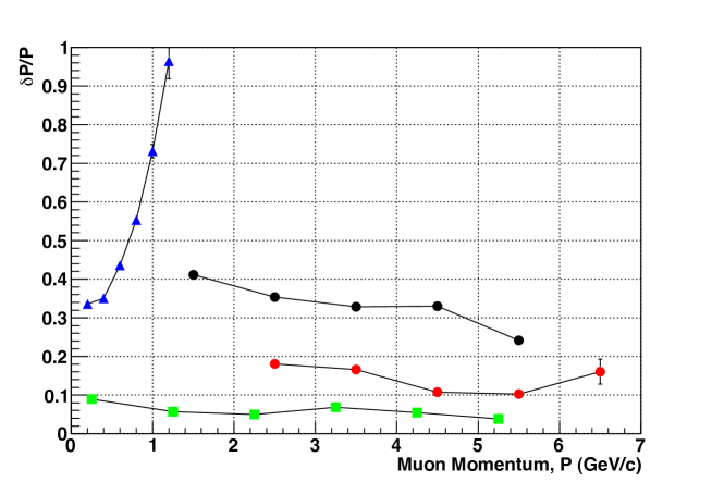
Figure 30: The obtained momentum resolution percentage including all the selection, efficiency and reconstruction procedures as described in the text. The blue dots correspond to the measure performed by the magnetic field in air, the red (black) dots correspond to what can be achieved by using the slope algorithm in the magnetic field in iron with the two (one) arms. The achievable resolution with the dE/dX range corresponds to the green dots.

In Fig. 31 we show the Spectrometer performance in terms of charge sign reconstruction. In the figure the separate contribution of muon bending in the air magnet and in the magnetized iron are shown.

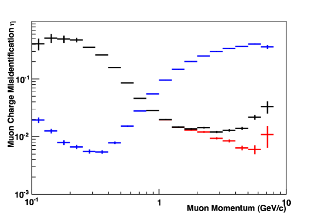
Figure 31: The obtained charge mis-identification percentage including all the selection, efficiency and reconstruction procedures as described in the text. The blue dots correspond to the measure performed by the magnetic field in air, the red (black) dots correspond to the magnetic field in iron with the two (one) arms.

Once the muon momentum is computed, the neutrino energy is estimated according to the event topology. For QE events the two-body kinematics allow a precise reconstruction of the incident neutrino energy from the measured momentum and direction of the outgoing muon:

$$E_{\nu}^{\rm rec}=\frac{1}{2}\frac{(M_{p}^{2}-m^{2}_{\mu})+2E_{\mu}(M_{n}-V)-(M_{n}-V)^{2}}{-E_{\mu}+(M_{n}-V)+p_{\mu}\cos{\theta_{\mu}}}$$ (13)

where $M_{p}$, $M_{n}$, $m_{\mu}$, $E_{\mu}$, $p_{\mu}$, $\cos{\theta_{\mu}}$ $V$ are the proton, neutron, muon masses, muon energy, momentum and angle with respect to the incoming neutrino direction and the LAr nuclear potential, set at 27 MeV, respectively. For non-QE events the neutrino energy is reconstructed adding up the muon energy to the energy of hadronic system, with a gaussian smearing $\sigma_{E}/E=0.3/\sqrt{E}$

A two-flavor sensitivity plot was computed assuming $\nu_{\mu}$ disappearance and a $\Delta\chi^{2}$ approach. We compared the FD measured neutrino spectrum with the non-oscillated spectrum derived from the ND data. We assumed a 5% overall systematic uncertainties on the absolute normalization derived from the ND spectrum. Fig. 32 shows the 90% C.L. sensitivity curve for the negative-focussing option assuming 3.5$\times$10⁶ pot with the iron magnet (the achievable exclusion limits by including also the magnet in air, are in progress).

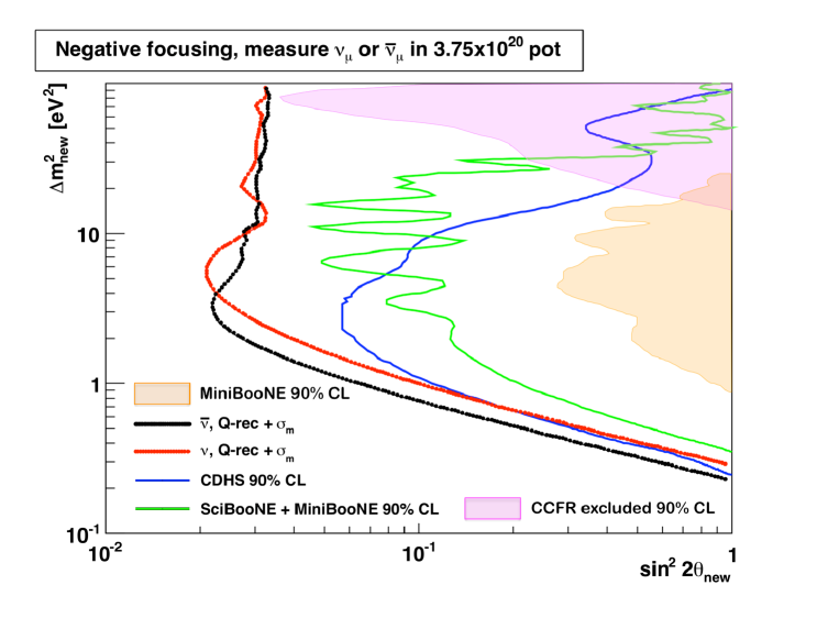
Figure 32: The sensitivity plot (t 90% C.L.) for the negative-focussing option assuming 3.5$\times$10⁶ pot with and without the air magnet option. Black (red) line: $\overline{\nu}_{\mu}$ ($\nu_{\mu}$)exclusion limit. Note that the contribution of the magnetic field in air to the sensitivity has not being included, yet. Blue (green) line: old (recent) exclusion limits on $\nu_{\mu}$ from previous (CDHS) and recent ([43])measurements.The two filled areas correspond to the present exclusion limits on the $\overline{\nu}_{\mu}$ from CCFR ([44] and MiniBooNE [16] experiments (at 90% C.L.).

The study of the possible physics performances of the Spectrometers with respect to the neutrino interactions inside the iron is in progress.

8 Mechanical Structure

The two OPERA iron dipole magnets [45] can be taken as an example for the design of NESSiE Spectrometers. They are made of two vertical walls with rectangular cross section and of the top and bottom flux return yokes, as shown in Fig. 33. Each wall is composed of 12 layers of iron slabs 5 cm thick, separated by 11 gaps, 2 cm thick, hosting RPC detectors.

The iron layers are made of 7 vertical slabs, for a total area of $(8.75\times 8.2)\mbox{m}^{2}$. Including the top and bottom return yokes, the total height of the magnet is about 10 m and its length along the beam 2.85 m. The magnet weight is around 1 $Kton$.

The slabs, the top and the bottom yokes are held together by means of screws, while more screws (about $1/\mbox{m}^{2}$) are used to keep slabs straight with spacers to ensure the thickness uniformity of the gaps hosting the detectors.

The Spectrometers are magnetized by coils located at the top and bottom return yokes, as shown in Fig. 33.

The installation of each magnet was performed according to the following time sequence:

• bottom yoke installation;

• internal support structure construction;

• iron/RPC layers installation (one plane in each arm at the time in order to keep the structure balanced);

• top yoke installation;

• removal of the internal structure.

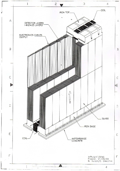
Figure 33: OPERA magnet scheme.

For the NESSIE experiment a very similar setup should be used to profit of the available detectors which have been designed to obtain the maximum acceptance coverage and the strip signal configuration. The different geometrical requirements for NESSiE corresponds to an equal width (7 vertical slabs) and a smaller total height (5 rows of RPC’s instead of 7) for the Far Spectrometer. The ND will instead be constructed with 5 vertical slabs of 3.4 m high. For the OPERA experiment a total of 336 slabs, (1.25*8.2) $m^{2}$ wide, were employed. Such slabs can be cut into the shape needed for the present baseline NESSiE configuration, but a new production will also be needed. The top and bottom returns must be redesigned and the copper coils modified accordingly.

9 Magnet Power Supplies and Slow Controls

The following description is based on the past experiences with the OPERA iron magnets (see [45] and references therein). Similar applications are foreseen for the present Proposal, with minor changes due to the magnetic field in air not present in OPERA and the thicker magnet.

9.1 Power Supply features

The magnetomotive force to produce the B field is provided by DC power supplies, located on the top of the magnet. They are single-quadrant AC$\rightarrow$DC devices providing a maximum current of 1700 A and a maximum voltage of 20 V. As a single-quadrant power supply can not change continuously the sign of the voltage, the sign of the current is reversed by ramping down the power supply and inverting the load polarity through a motorized breaker. The power supplies are connected to the driving coil wound in the return yokes of the magnet by means of short flexible cables.

Ancillary systems

• Coil: The coil is made of $100\times 20mm^{2}$ copper (type Cu-ETP UNI 5649-711) bars. The segments are connected through bolts after polishing and gold-plating of the contact surface. Each coil has 20 turns in the upper return yoke connected in series to 20 more turns in the bottom yoke. The two halves are linked by vertical bars running along the arm. Rexilon supports provide spacing and insulation of the bars.

• Water cooling: Water heat exchangers are positioned between these supports and the bars while the vertical sections of the coil are surrounded by protective plates to avoid accidental contacts. More than 160 junctions have been made for each coil and the quality of such contacts was tested measuring the overall coil resistance during mounting. Cooling ensures an operating temperature of the RPC detectors lower than 20⁰ C.

Current status of the two OPERA power supplies

Even if the 1^rst power supply stops with a monthly frequency the 2^nd power supply is instead working without troubles. Altogether the overall downtime of the two OPERA magnets is about 0.1%.

A similar framework is foreseen for the NESSiE proposal. Both the Far and the Near magnets will need a single power supply each.

9.2 Monitored quantities for every magnet

Here is the list of the foreseen values to be monitored:

• continuous measurement of the magnetic field strength by Hall probes or pickup coils at magnet ramp down (not routinely done in OPERA)

• electrical quantities:

  1. current: check for maximum / minimum range

  2. voltage: check for maximum / minimum range

  3. ground leakage current: check for maximum range (not automatically done in OPERA, via web cam or onsite check)

• temperatures and cooling:

  1. coil temperatures: check for maximum range

  2. cooling water input temperature: check for maximum / minimum range

  3. cooling water output temperature: check for maximum / minimum range

  4. cooling water pressure, cooling water flux: check for maximum / minimum values (not automatically done in OPERA, via web cam or onsite check).

9.3 Slow Control

The slow control system of the Spectrometer will be developed to master all the hardware related: the magnet power supplies, the active detectors and all the ancillary systems.

According to the experience acquired for the OPERA experiment [46] the system is organized in tasks and data structures developed to acquire in short time the status of the detector parameters which are important for a safe and optimal detector running.

The slow control should provide a set of tools which automatize specific detector operation (for instance ramping up of the detector High Voltage before the start of a physics run) and lets people on shift control the different components during data taking.

Finally, the slow control has to generate alarm messages in case of a component failure and react promptly, without human intervention, to preserve the detector from possible damages. As an example the RPC High Voltages have to be ramped down in case of any failure of the gas system.

A possible structure of the slow control can be organized as follows:

• one databases is the heart of the system; it is used to store both the slow control data and the detector configurations.

• the acquisition task is performed by a pool of clients, each serving a dedicated hardware component. The clients are distributed on various Linux machines and store the acquired data on the database.

• the hardware settings are stored in the database and served through a dynamic web server to all the clients as XML files. A configuration manager gives the possibility to view and modify the hardware settings through a Web interface.

• a supervisor process, the Alarm Manager, which retrieves fresh data from the database, and is able to generate warnings or error messages in case of detector malfunctioning.

• the system is integrated by a Web Server which allows controlling the global status of data taking, the status of the various components, and to view the latest alarms.

10 Detectors for the Iron Magnets

The Near and Far Spectrometers of NESSiE will be instrumented with large area detectors, ND and FD respectively, for precision tracking of muon paths allowing for high momentum resolution and charge identification capability. According to Fig. 26 a resolution of the order of $1\ mm$ is needed for the low momentum muons crossing the magnetic field in air. A resolution of about $1\ cm$ is instead enough for the large mass detectors that we plan to use within the iron slabs of the Spectrometers. In this Section we focus on the latter whilst several different options will be described in the next Section for the high resolution detectors which have to be used in the “air” part.

Suitable active detectors for the ND and FD Iron Spectrometers are the RPC - gas detectors widely used in high energy and astroparticle experiments [47] - because:

• they can cover large areas;

• are relatively simple detectors in terms of construction, flexibility in operation and use;

• their cost is cheaper than other other large area tracking systems;

• they have excellent time resolution;

• and large counting rate power (in specific operational modes).

Furthermore a large part of the units to be used are already available. In fact by considering the remainders of the OPERA RPC production, about $1500\ m^{2}$ of RPC’s can be used.

10.1 RPC’s detectors

We plan to use standard bakelite RPC : two electrodes made of 2 mm plastic laminate kept 2 mm apart by polycarbonate spacers, of 1 cm diameter, in a 10 cm lattice configuration. The electrodes will have high volume resistivity ($10^{11}-10^{13}\Omega$ cm). Double coordinate read-out is obtained by copper strip panels. The strip pitch can be between 2 and 3.5 cm in order to limit the number of read-out channels over a large area. An optimization of the strip size and orientation (horizontal, vertical and tilted ones) is required in order to define the best performances of the Spectrometer (track reconstruction resolution and reduction of ghost hits). RPC’s are commonly used in streamer mode operation with a digital read-out as described in the following.

10.2 Ancillary systems

For the operation of the RPC’s in the Spectrometer, ancillary systems are needed, namely:

• a Gas distribution system;

• a High Voltage system with current monitoring performed by dedicated nano-amperometers designed by the Electronics Workshop of LNF.

• monitoring of several environmental/operational parameters (RPC temperatures, gas pressure and relative humidity).

10.3 The Gas system

Since the overall rate (either correlated or uncorrelated) is estimated to be low (see Sect. 12), standard gas mixtures for streamer operation can be used, like for instance the one employed in the OPERA RPC’s, composed of Ar/tetrafluorethane/isobutane and sulfur-hexafluouride in the volume ratios: 75.4/20/4/0.6.

Different gas mixtures can be further investigated and an optimization is advisable in view of the DAQ system adopted (digital versus analog read-out) and the safety regulations in the experimental halls. OPERA RPC’s are flushed with an open flow system at 1500 l/h corresponding to 5 refills/day. The installation of a recirculating system could also be considered, if the gas flow has to be increased to prevent detector aging.

10.4 The Tracking Detectors for the Near and Far Spectrometers

The design and evaluation of the requirements for the two detectors are base on the RPC’s developed for the OPERA experiment at LNGS. Each of its unit of RPC owns dimensions of $2904\times 1128\ mm^{2}$.

The Near Spectrometer will have a magnetic field in air followed by a calorimeter of interleaved planes of iron and RPC. In the ND RPC’s will be arranged in planes of 2 columns and 3 rows for a total exposed surface of about 20 m². A total of 40 planes will instrument the Spectrometer and a total of 720 $m^{2}$ of detectors are thus required. Taking into account the RPC dimensions, this number corresponds to 240 units.

The Far Detector design will be very similar to the one conceived one for the magnetized Iron Spectrometers of the OPERA experiment. The detector will consist of units arranged in 3 columns and 5 rows to form planes of about 50 $m^{2}$. As for the Far magnet 40 planes of detectors will be interleaved with iron absorbers for a total of about 1800 $m^{2}$ (600 units).

10.5 Production and QC tests

OPERA RPC’s, before the installation, underwent a full chain of quality control tests serialized in the following steps:

• mechanical tests (gap gas tightness and spacers adhesion);

• electrical tests;

• efficiency measurement with cosmic rays and intrinsic noise determination.

The setup, still partially available at Gran Sasso INFN Laboratories, was able to validate about 100 m² of RPC’s per week.

10.6 Costs

Plastic laminate can be produced in Italy by Pulicelli, a company located near Pavia (the company is currently producing material for the CMS RPC upgrade system). The cost of plastic laminate is about 30 €/$m^{2}$. The RPC chamber assembly can be done in Italy by the renovated General Tecnica company with an estimated cost of about 300 €/$m^{2}$. The overall cost of a complete new RPC production is foreseen in about 1.5 M€.

As for the read-out strips, the costs for 5000 m² is around 500 K€.

11 Detectors for the Air Magnet

The air-core magnet (Sec. 5.2) will be used for the charge identification of low momentum muons which requires precise measurements of the muon path. A (4$+$4)-layers tracker was simulated (see left plot in Fig. 34) assuming a $0.25\ T$ magnetic field of in between. Track reconstruction is required only in the bending plane (XZ). The identification of the muon charge is optimized looking at the change of the track slope before and after the magnetic field. Different detector resolutions were simulated (see right plot in Fig. 34) and a resolution of the order of $1\ mm$ results as the proper choice.

Several detector options for such precise measurements are briefly discussed in the following. More detailed MC simulations and eventual test-beams will be crucial to test the capability of the different detectors to reach the required performances. The final choice on these precision trackers will depend also on the cost, on the reliability and on the possibility of re-using parts from previous experiments.

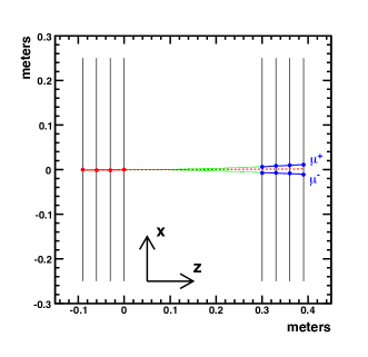
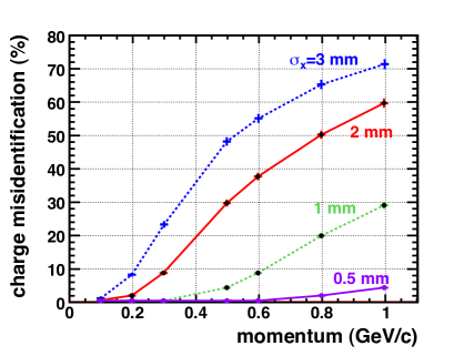
Figure 34: Left: Display of a simulated event with momentum $p=500\ MeV/c$ in the air-core magnet. Right: the charge mis-identification percentage as a function of the muon momentum for different detector resolutions (incoming muons perpendicular to the detector plane). The slope difference was used to measure the charge.

11.1 Drift tubes (OPERA-like)

In the OPERA experiment the High Precision Trackers (HPT’s) are mainly devoted to muon identification and charge measurement. HPT’s are drift chambers (aluminum tubes each with a central sense wire) arranged in fourfold layers in order to avoid ambiguities in the track reconstruction and to enhance the acceptance (see example in Fig. 35). In order to simplify the calibration procedures the wires have been located by using cover plates and the wire position is decoupled from the position of the tube. Thus a wire position accuracy has been achieved with a tolerance of $0.1\ mm$. In this configuration and assuming negligible inefficiency, the spatial single tube resolution (rms) has been measured to be better than $0.3\ mm$.

The main features of these gas devices are mechanical robustness, absence of glue to retain the gas quality, signal quality guaranteed by a Faraday cage. In the OPERA detector the HPT’s are grouped in modules and the layers are staggered to optimize the acceptance and to minimize the left/right ambiguities. The tubes are filled with a gas mixture ($80\%\ Ar$, $20\%\ CO_{2}$) and run at a pressure of $1005\ mbar$. TDC units with a Least Significant Bit of $1.5\ ns$ are used to measure the drift time (the time spectrum ranges up to $1.6\ \mu s$ and TDC’s cover a double range).

The large size ($8\times 8\ m^{2}$) has been the main challenge in designing the OPERA detector, with vertical tubes of $\sim 8\ m$. The HPT size is not a problem in designing the NESSiE vertical precise trackers because $3\ m$ and $5\ m$ (vertical dimensions) are enough for Near and Far detectors, respectively, and the reduced size could allow the complete re-use of the OPERA HPT’s.

Figure 35: Four layers of staggered drift tubes allow reconstructing the track without ambiguities.

11.2 RPC’s with analog read-out

Resistive Plate Chambers (RPC’s) are gas detectors [47] widely used in high energy and astroparticle experiments. A single gas-filled gap delimited by bakelite resistive electrodes is the simplest set-up commonly used in streamer mode and digital read-out. We already introduced them in Sect. 10.1. The most relevant features are the excellent time resolution and the high rate capability. Also the position resolution is very good, in particular conditions the centroid of the induced charge profile was determined [48] with a FWHM resolution of $\sim 0.12\ mm$. In the case of the NESSiE experiment such resolution is not necessary and simpler and cheaper set-up can be used.

The analog read-out of RPC has been implemented in the last years [49] or variously proposed. With this technique by reading the total amount of charge induced on the strips detailed information can be obtained on the streamer charge distribution across the strips and better estimate of the track across the detector is thus achieved than in the digital case. The charge profile can be approximated by a Gaussian shape whose width ($\sim 5\ mm$) does not depend on the gas mixture and operating high voltage, unlike the total charge which is strongly dependent on them (see Fig. 36).

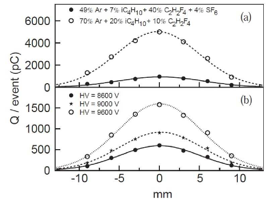
Figure 36: Charge profile (normalized per event) observed with RPC working in streamer mode: (a) for various gas mixtures at nominal running HV, (b) for different high voltages with the gas mixture ($49\%Ar+7\%iC_{4}H_{10}+40\%C_{2}H_{2}F_{4}+4\%SF_{6}$) foreseen for the ALICE detector. The curves are Gaussian fits of the data. The standard deviation of these distributions is about $5\ mm$ in all cases [51].

A few $mm$ resolution in the charge position determination is obtained by choosing an adequate strip size. Also the dynamic range is improved, allowing the detection of particles at a density of the order of $1000\ particles/m^{2}$.

11.3 RPC’s with digital read-out in avalanche regime

Another possibility is to operate the RPC’s in avalanche mode: the incoming particles release primary charges followed by Townsend avalanches in the gas gap.

The bidimensional measurement of the avalanche position with $mm$-accuracy has been verified in single-gap chambers [52]. As in avalanche regime the charge cluster size results to be smaller by some order of magnitude with respect to the streamer mode operation (it depends on HV and gas mixture), it is possible to achieve better space resolution by using smaller digital strips. A higher rate capability is also attainable due to the lower amount of charge delivered in the avalanche. The response of standard $2\ mm$ gap RPC’s in streamer mode can not be higher than $3\ MHz/m^{2}$, while in avalanche mode it can attain $30\ MHz/m^{2}$.

It is also possible to use the RPC in saturated avalanche mode. The advantage is to have a lower charge signal than in streamer mode but still high enough to remove the need for a pre-amplifier. Analog read-out with an optimized strip size guarantees an adequate position resolution.

Anyway the avalanche mode has the inconvenient of being more sensitive to temperature and pressure variability due to the lower amount of charge produced.

Finally, regarding the possibility to get high precision position measurement with RPC’s at a sustainable cost, a new procedure has been developed to determine the charge position by timing measurements. Precision in the sub-millimeter range has been reached [53]. The method is based on the read out of the signal propagating in the graphite. The graphite electrode, coupled to the ground reference of the detector read-out panels, is a distributed capacitance-resistance system (see Fig. 37). The occurrence of a discharge in the gas produces a point-like perturbation of the steady potential distribution of the system. The time behaviour of the perturbation can be described, in the approximation of infinite electrode size, by a two-dimensional Gaussian distribution with time dependent variance and amplitude. The distance is related to the time (of the maximum) by a quadratic relation which can be used to measure the position from the time measurement. The sharpness of the maximum is strongly dependent on the distance. A distribution with a FWHM of $0.8\ mm$ has been reached.

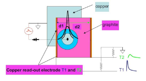
Figure 37: Pick-up scheme in the graphite electrode. From [53].

12 Backgrounds

Assuming neutrino fluxes as described in Sect. 4 around 10-15 events per spill are expected in the Near Detector, a spill being 2.1 $\mu s$ long within a cycle of 1.2 $sec$. For the Far Detector the rate of events is reduced by about a factor of 20.

The possible background rates are analyzed assuming a tracking system with single-gap RPC’s. We distinguish the uncorrelated background due to detector noise and local radioactivity (dark counting rate) and the correlated background due to cosmic rays.

12.1 Uncorrelated background

The dark counting rate depends on detector features and ambient radioactivity. A typical value for RPC as measured at sea level is $300\ Hz/m^{2}$. Therefore the expected rate per plane is $\lambda_{N}=300\ Hz/m^{2}\times(3\times 6\ m^{2})\simeq 5.4\ kHz$ on the Near Spectrometer and $\lambda_{F}=300\ Hz/m^{2}\times(5\times 9\ m^{2})\simeq 13.5\ kHz$ on the Far Spectrometer. Assuming a read-out time window of $10\ \mu s$ we expect 0.05 (0.14) hits per RPC plane per event on the Near (Far) detector. The number of fired strips will depend on the strip width (in OPERA with $2.6$ and $3.5\ cm$ strip-wide the typical cluster size is $\sim 1.5$ strips).

The requirement of three-contiguous-planes coincidence in the beam-spill time (tipically $2\ \mu s$) makes the dark noise contribution to the trigger rate negligible (see last column in Tab. 8).

12.2 Cosmic Ray background

The contribution of Cosmic Rays (CR) to the plane-by-plane background is similar to that discussed in the previous Section, but CR events yield long tracks that constitute a potentially more dangerous correlated background.

Assuming a trigger majority of at least 3 fired planes a cosmic particle can trigger the data-taking when it has enough energy to cross 2 iron slabs ($2\times 5\ cm$). The CR flux at sea level is essentially due to muons (hard component of Extensive Air Showers) and these particles can trigger the data-taking when their momentum exceeds $250\ MeV/c$. Then the integrated vertical flux of muons is $J=97\ Hz/m^{2}/sr$ at sea level [54].

The integrated vertical flux of the soft component (electrons and positrons) can be represented by $J(>E)=0.22\ E^{-1.45}\ [Hz/m^{2}/sr]$, where $E$ is in $GeV$. Taking into account this contribution and minor ones due to hadrons, $J=100\ Hz/m^{2}/sr$ will be used in the following calculations as integrated vertical CR flux at sea level.

In the conservative hypothesis that the CR ray flux is isotropic above the horizon and equal to the vertical flux, the total rate $\lambda_{RC}$ on a detector shaped as a fully efficient box is

$$\lambda_{RC}=\frac{\pi}{2}S_{tot}J$$

where $S_{tot}$ is the surface of the detector. The expected number of CR events in a time window of $2\ \mu s$ (the beam-spill time) is reported in Tab. 8. They scale with the time window $T$ (by a factor $T/2\ \mu s$). The data in Tab. 8 conservatively ignore that more detailed trigger conditions allow a significant reduction of the background.

	Dimensions	Surface	Total Iron Mass	CR events	Dark noise ev.
	($m\times m\times m$)	($m^{2}$)	($ton$)	in $2\ \mu s$	in $2\ \mu s$
Near	$6\times 3\times 5$	126	364	$4\times 10^{-2}$	$2\times 10^{-4}$
Far	$9\times 5\times 5$	230	846	$7\times 10^{-2}$	$3\times 10^{-3}$

Table 8: Dimensions and surfaces of the detectors, iron masses and estimated background events (CR and dark noise) for the Near and Far Spectrometers.

13 Read-out, Trigger and DAQ

13.1 DAQ overview

The aim of the DAQ is to read the signals produced by the electronic detectors and to create a database of detected events. We recall in Table 9 the characteristics of the CERN PS primary proton beam. These are important inputs to define properly the data acquisition and flow.

Table 9: Characteristics of the PS primary proton beam.

	PS Parasitic	PS Dedicated
Proton beam momentum	20 GeV	20 GeV
Protons per pulse	$2.6\times 10^{13}$	$3\times 10^{13}$
Number of bunches	7	8
Bunch length (4 sigmas)	65 ns	65 ns
Bunch spacing	262 ns	262 ns
Burst length	1.8 $\mu$s	2.1 $\mu$s
Maximum repetition rate	1.2 s	1.2 s
Beam energy	84 kJ	96 kJ
Average beam power	70 kW	80 kW

The foreseen DAQ architecture is composed of three stages:

• the front end electronics close to the detector (FEB)

• the read-out interface which together with the trigger board control the read-out of the FEB

• the Event Building which reconstructs events using standard workstations.

The whole event reconstruction is based on the time correlation of the channels, which depends on the accuracy of the electronic channels time stamping. A time resolution in the range $5\div 10\ ns$ is sufficient to correctly associate the different hits to the corresponding events. A common time reference with respect to the PS extraction time is used to time-stamp the data and to correlate the events recorded by the Spectrometer to the data recorded in LAr.

13.2 Data Flow

The Far detector is designed with 15 RPC/plane $\times$ 20 planes/arm times 2 arms for a total of 600 RPC detectors, 3 $m^{2}$ each. The Near detector is designed with 6 RPC/plane $\times$ 20 planes/arm times 2 arms for a total of 240 RPC’s.

Assuming a strip size of 2.6 cm along Y and 3.5 cm along X for the Far detector each plane will be equipped with $32\times 5=160$ horizontal strips plus $112\times 3=336$ vertical strips for a total number of about 500 electronic channels per plane. The total number of channels is therefore about 20,000. For the Near detector the number of electronic channels will be about 300 per plane. The total number of channels is about 12,000.

Given the expected background rate due to the RPC single rate and the counts due to cosmic ray within the beam spill reported in Sect. 12, the expected data rate is dominated by the beam related events. With a maximum PS beam intensity of $3\times 10^{13}\leavevmode\nobreak\ \mbox{p.o.t.}$ about 10 to 20 events are expected in the Near detector. Assuming four hit strips per plane and at most $16\leavevmode\nobreak\ byte$ of data per hit (channel address, signal and time) the size of the event after zero suppression is expected to be $1\leavevmode\nobreak\ kbyte$.

13.3 Front-End Electronics

The role of the electronic read-out is to discriminate the signals coming from the RPC’s strips and to record the signals above threshold. The start-of-burst signal will be used as a trigger and discriminated signals will thus be recorded during the whole burst duration. A time-stamp with a resolution of $5\div 10\leavevmode\nobreak\ ns$ will allow associating hits belonging to the same events.

The electronic read-out of the RPC’s could be developed according to the same design scheme adopted for the OPERA experiment, where they are operated in streamer mode and read-out by means of twisted pair cables; these are in turn connected to special interconnection boards allowing the front-end electronics to be placed far from the detector. The Front-end Boards (FEB) collect signals from RPC’s strips and deliver them to a Controller Board (CB) acting as an interface to the DAQ system.

About 32,000 channels will be used to read-out 2,500 $m^{2}$ of RPC detectors with pickup strips of $2.5\ cm$ pitch in the vertical direction (orthogonal to the bending plane) and $3.5\ cm$ pitch in the horizontal direction (tracking without bending). Each FEB board will collect signals from 64 strips providing discrimination, time stamping and local buffering sized to store up to 40 events per burst. The local buffer will be read-out from the CB, during the inter-spill time, lasting 1.2 $s$. Serial FEB data transfer to the CB will occur at a clock of 10 MHz, taking a few hundred microseconds. A new ASIC front-end chip will be designed to assign the time-stamp to each event and make it possible to record multiple events in the same burst. The possibility to have a double electronic chain, digital and analog, for each channel will be considered. In the ASIC project a 10-bit ADC with a multiplexing and sample-and-hold system allowing for the analog read-out could be added. The design of this new ASIC chip can be provided by the INFN electronics CAD service.

The cost estimation, based on a production of 2,500 16-channel chips, amounts to 30 €/chip. The production cost of 700 Front-End Boards, including additional components and assembly, has been estimated to be about 50 €/board. The production of 100 VME Controller-Board has been estimated to be 300 €/board. Additional costs: cables and connectors 20 K€, low voltage power supply 20 K€, crates 30 K€. The total cost of the RPC’s read-out electronics has been estimated to be 210 K€, taking into account 32000 digital channels plus some contingency.

13.4 DAQ

The acquisition for each detector (FD/ND) is composed by Front-End Boards (about 5 FEB per plane), Trigger Boards, Controller Boards (1 CB per plane) and the Event Builder. In order to acquire with a rate of 10 to 20 events/spill (each spill is 2.1 $\mu s$ long), Front-End Boards should provide a pipeline system to save all the data of a spill, provide a FAST_OR signal for trigger purposes of granularity in the range between 8 and 32 strips and perform the zero suppression. The possibility of a digital or analog read-out must be envisaged. The start of the pipeline should be given by the start of the spill and the time resolution should be in the range 5 - 10 $ns$.

The Trigger Boards should process the FAST_OR signals from the Front-End Boards and provide an external trigger condition to the Front-End Boards. This signal could also be used as an external trigger for the High Precision Tracker read-out ($t_{0}$ signal for the TDC). A Trigger Bus should be implemented for the distribution of the trigger. Given the expected overall rate (beam events, cosmic, single rate) and due to the Front-End Boards buffer a trigger signal based only on the beam spill could be envisaged.

The Controller Boards should read-out the signals from the Front-End Boards and propagate them to the Event Building which is receiving data from the Spectrometer and the High Precision Tracker systems. The Event Building is using standard network protocols.

Data read-out and Event Building should be performed in the time between two spills ($\sim 1.2s$). The Event Builder should be based on standard commercial workstation. Data spying and monitoring process will also be implemented at this level.
The correlation between Spectrometer and LAr data is achieved using a common clock signal to time-stamp the events. Data merging is performed offline at the reconstruction level.

14 CERN Logistics

The two experimental halls identified in the LAr proposal (see Sect. 3 of [1]) to host the Near and Far detectors, B181 and B191, respectively, are well suited for the two Spectrometers too. The two halls have been chosen to be in the line of the PS neutrino beam and to fit the size of the detectors. Some discussion is undergoing with CERN for the use of the chosen pit in hall B181, already exploited by some servicing. As the pit would not actually fit both the LAr and the Spectrometer detectors and some excavation works will be anyhow needed, a different solution is in addition under study. A new pit in a new hall in front or behind B181 may be constructed.

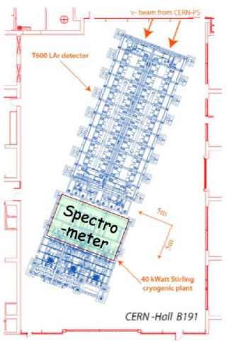
Figure 38: The general layout of the Hall B-191 at CERN that is supposed to host the Far detectors, LAr and Spectrometer. The Spectrometer is placed behind the LAr tanks and overlays the cryogenic plant, which has to be moved e.g. on the right side. The direction of the neutrino beam is also indicated on the top of the picture.

For the Far site (see Fig. 38) the Spectrometer detector can easily be allocated behind the two Icarus tanks in case the cryogenic equipment be allocated laterally. The total weight for the magnet will exceed 1 K$ton$, on an extension of less than 40 $m^{2}$. Therefore the floor has to be eventually adapted. As described in Sect. 8 the installation of the magnets has to follow a precise time sequence which has to be compatible with the LAr installation and contemporary allow for the closest positioning of Spectrometer and LAr. Detailed engineering studies will take care of this subject.

15 Schedule and Costs

The choice of performing a design study that is reliable under several aspects led to make conservative, well controlled and realistic options. In particular the choice to use detectors like the RPC ones and the development of dipole magnets which had, at least partly, already been constructed and are in use, allows us to keep under control both the time schedule and the costs.

With respect to the schedule, which is reported in Tab. 10, it should be underlined that is based on the deep experience acquired with the OPERA Spectrometers, built up from 2005 to 2006 under critical conditions.

Year(portion)	Action
2012	Design optimization
1rst half 2013	Define tenders/contracts
	Setting up Detectors Test-stands
2nd half 2013	Mechanical Structure construction
	Detector production
	Start Detector test
	Magnet (Air) preparation
1rst half 2014	Start Magnet installation
	Start detectors installation
2nd half 2014	End installation

Table 10: Tentative time schedule for the 2012-2014 years which will include the final optimization of the detectors, their construction and installation at CERN.

With respect to the cost estimate, the expenses needed for the major items are reported in Tab. 11.

Item	Cost (in M €)
Far
Magnet	2.5
Detectors	1.0
Strips	0.5
Data Acquisition	1.0
Near
Magnet	2.0
Detectors	0.5
Strips	0.3
Data Acquisition	0.5
Total	8.3

Table 11: Estimate of the costs of the major items.

The partial re-use of systems developed for the OPERA experiment may be envisaged in case that experiment would not need them anymore at the time of the construction. We note that the OPERA Spectrometers have been fully funded by INFN, except the Precision Trackers, which is therefore committed to their dismantling and entitled to possibly re-use as well. To this respect, it is clear that e.g. the iron raw material will be available sooner or later to INFN which may then take it into account for company arrangements.

16 Conclusions

Existing anomalies in the neutrino sector may hint to the existence of one or more additional sterile neutrino families. We performed a detailed study of the physics case in order to set a Short-Baseline experiment at a refurbished CERN-PS neutrino beam, able to either prove or reject the existence of sterile neutrinos.

The already submitted proposal based on the technology of imaging in ultra-pure cryogenic Liquid Argon (LAr) may suffer from some experimental limitations which we deem critical: the measurement of the muon charge on event-by-event basis extended to the lowest achievable energy range would be mandatory. Indeed the muon leptons from Charged Current (CC) (anti)-neutrino interactions play an important role in disentangling different phenomenological scenarios, provided their charge state is determined. Since CC muon events induced by the primary beam would be very abundant, a search based on muon appearance-disappearance will benefit of large statistics.

The best option in terms of physics reach and funding constraints is provided by two Spectrometers based on dipoles magnets mostly in iron, at the Near and Far sites (located at 127 and 850 $m$ from the CERN PS neutrino beam, respectively), to be placed behind the LAr detectors.

In order to measure the momentum and identify charge with high sensitivity in an extended energy range (from few hundred $MeV$ to above 5 $GeV$) we complement the iron-core dipole by a magnetic field in air in a limited region just in front.

The selected detectors, mainly Resistive Plate Chambers, would exploit well known technologies and make it possible to re-use part of existing ones (should they become available; if not, it would imply an increase of the costs with no additional delay).

The Near and Far Spectrometers by complementing the capabilities of the LAr detectors will fully exploit the very rich and exciting physics information in case sterile neutrinos indeed exist. In fact the Spectrometers by measuring the momentum and identifying the charge of the muons will provide valuable information in:

• measuring $\nu_{\mu}$ disappearance in the full momentum range which is a key ingredient in rejecting the anomalies or measuring the whole parameter space of oscillations involving sterile neutrino;

• measuring the neutrino flux in the Near detector, in the full muon momentum range, which is quite relevant to keep the systematic errors low.

The measurement of the muon charge will furthermore provide valuable information in:

• separating $\nu_{\mu}$ from $\overline{\nu}_{\mu}$ in the antineutrino beam where the $\nu_{\mu}$ contamination is quite important. This measurement is critical to fully exploit the experimental capability of measuring a difference between $\nu_{\mu}\rightarrow\nu_{e}$ and $\overline{\nu}_{\mu}\rightarrow\overline{\nu}_{e}$ difference in view of a possible signature of CP violation.

Results of our study are reported in detail in this proposal where our experiment is identified with the acronym NESSiE (Neutrino Experiment with SpectrometerS in Europe).

References

- [1] LAr Proposal SPSC-M-773, submitted on March 9th 2011.
- [2] LSND Collaboration, A. Aguilar et al., “Evidence for Neutrino Oscillations from the Observation of Anti-Neutrino(electron) Appearance in a Anti-Neutrino(muon) Beam”, Phys. Rev. D64, 112007 (2001), hep-ex/0104049.
- [3] C. Giunti, M. Laveder, “Statistical Significance of the Gallium Anomaly” Phys. Rev. C83, 065504 (2011) arXiv:1006.3244.
- [4] T. Mueller et al., “Improved Predictions of Reactor Anti-Neutrino Spectra”, Phys. Rev. C , 1101.2663 (2011).
- [5] CDHS Collaboration, F. Dydak et al., “A Search for Oscillations in the range 0.390 ”, Phys. Lett. B134, 281 (1984).
- [6] C. Giunti and M. Laveder, “Short-Baseline Electron Neutrino Disappearance, Tritium Beta Decay and Neutrinoless Double-Beta Decay”, Phys. Rev. D82, 053005, (2010) arXiv:1005.4599.
- [7] G. Mention et al., “The Reactor Anti-Neutrino Anomaly”, (2011) hep-ex/arXiv:1101.2755.
- [8] G. Mangano, A. Melchiorri, O. Mena, G. Miele, and A. Slosar, “Present bounds on the Relativistic Energy Density in the Universe from Cosmological Observables”, JCAP 0703, 006 (2007), astro-ph/0612150.
- [9] A. Melchiorrri, “Sterile neutrino constraint from cosmology”, Talk at Beyond3nu, LNGS, 3-4/05/2011, see slide # 23.
- [10] C. Giunti and M. Laveder, “VSBL Electron Neutrino Disappearance”, Phys. Rev. D80, 013005, 0902.1992 (2009).
- [11] MiniBooNE Collaboration, A. Aguilar-Arevalo et al., “A Search for Electron Neutrino Appearance at the eV2 scale”, Phys. Rev. Lett. 98, 231801 (2007), arXiv:0704.1500.
- [12] MiniBooNE Collaboration, A. Aguilar-Arevalo et al., “A Search for Electron Anti-Neutrino Appearance at the Delta m**2 1-eV**2 Scale”, Phys. Rev. Lett. 103, 111801 (2009), arXiv:0904.1958.
- [13] J. Kopp, M. Maltoni, and T. Schwetz, “Are there Sterile Neutrinos at the eV scale?”, arXiv:1103.4570, (2011).
- [14] C. Giunti and M. Laveder, “Hint of CPT Violation in Short-Baseline Electron Neutrino Disappearance”, Phys. Rev. D82, 113009 (2010), arXiv:1008.4750.
- [15] KARMEN Collaboration, B. Armbruster et al., “Upper limits for Neutrino Oscillations from Muon Decay at rest”, Phys. Rev. D65 112001, (2002), hep-ex/0203021.
- [16] MiniBooNE Collaboration, A. Aguilar-Arevalo et al., “A Search for Muon Neutrino and Anti-Neutrino Disappearance in MiniBooNE”, Phys. Rev. Lett. 103, 061802 (2009).
- [17] M. Maltoni, T. Schwetz and J.W.F. Valle, “Cornering (3+1) Sterile Neutrino Schemes”, Phys.Lett. B518 252 (2001), hep-ph/0107150.
- [18] LEP Collaboration (ALEPH, DELPHI, L3, OPAL), Alexander, G. and others, “Electroweak Parameters of the Resonance and the Standard Model”, Phys. Lett., B276, 247 (1992).
- [19] M. Maltoni and T. Schwetz, “Sterile Neutrino Oscillations after first MiniBooNE results”, Phys. Rev. D76, 093005 (2007), 0705.0107.
- [20] K. Schreckenbach, G. Colvin, W. Gelletly, and F. Von Feilitzsch, “Determination of the Anti-Neutrino Spectrum from U-235 Thermal Neutron Fission Products up to 9.5-MeV”, Phys.Lett. B160, 325 (1985).
- [21] G. Karagiorgi, Talk at Laguna Meeting of 03/04/2011.
-
[22]
BUGEY Collaboration, Y. Declais, H. De Kerret, B. Lefievre, M. Obolensky and A. Etenko et al.,
“Study of Reactor Anti-Neutrino Interaction with proton at Bugey nuclear power plant”,
Phys. Lett. B338 383 (1994).
Y. Declais, J. Favier, A. Metref, H. Pessard and B. Achkar et al., “Search for Neutrino Oscillations at 15-meters, 40-meters, and 95-meters from a nuclear power reactor at Bugey”, Nucl. Phys. B434 503 (1995). - [23] CHOOZ Collaboration, M. Apollonio et al, “Search for Neutrino Oscillations on a Long Base-Line at the CHOOZ nuclear power station”, Eur. Phys. J. C27, 331 (2003), hep-ex/0301017.
- [24] Giunti, C. and Laveder, M., “3+1 and 3+2 Sterile Neutrino Fits”, arXiv:1107.1452 (hep-ph), 2011.
- [25] C.Andreopoulos et al., “The GENIE Neutrino Monte Carlo Generator, Nucl. Instrum. Meth. A614, 87 (2010).
- [26] NOMAD Collaboration, P. Astier et al., “Search for Oscillations in the NOMAD Experiment”, Phys. Lett. B570 19 (2003), hep-ex/0306037.
- [27] E. K. .Akhmedov, T. Schwetz, “New MiniBooNE Results and non-standard Neutrino Interactions”, Nucl. Phys. Proc. Suppl. 217 217 (2011).
- [28] C. Giunti, M. Laveder, “Short-Baseline Oscillations”, Phys. Rev. D82 093016 (2010), arXiv:1010.1395.
- [29] C. Giunti, M. Laveder, “Large Short-Baseline Disappearance”, Phys. Rev. D83 053006 (2001) arXiv:1012.0267.
-
[30]
M. Baldo-Ceolin et al., CERN/PSCC/80-130, PSCC/P33, 30-10-1980;
C. Angelini et al. [PS180 Coll.], Phys. Lett. B179 307 (1986). - [31] M. Guler et al. (I216/P311 Proposal) 1999, “Search for Oscillation at the CERN PS”, Tech. Rep. CERN-SPSC/99-26, SPSC/P311.
- [32] I216/P311 LoI, CERN/SPSC/97-21.
- [33] G. Battistoni et al., “The FLUKA code: Description and Benchmarking”, AIP Conf. Proc. 896, 31 (2007).
- [34] A. Longhin. “A new Design for the SPL-Fréjus Super-Beam”, arXiv:1106.1096.
- [35] R. Santacesaria, private communication.
- [36] K. Anderson et al., FERMILAB-DESIGN-1998-01(1998).
- [37] http://info-psnf.web.cern.ch/info-PSNF/Presentations.
- [38] E. Gschwendtner, “The CNGS, Operation and Perspectives”, CERN, presentation at SBNW11, 12-14 May 2011, Fermilab.
- [39] W.T. Scott, “Correlated Probabilities in Multiple Scattering”, Phys. Rev. 76 212 (1949).
- [40] R.L. Gluckstern, “Uncertainties in Track Momentum and Direction due to Multiple Scattering and Measurement Errors”, Nucl. Instr. and Meth. 24 381 (1963).
- [41] W. Innes, “Some Formulas for Estimating Tracking Error”, Nucl. Instr. and Meth. in Phys. Res. A 238 (1993).
- [42] COMSOL is a commercial product, see www.comsol.com
- [43] MiniBooNE-SciBooNe Collaborations, K. B.M. Mahn et al., “Dual Baseline Search for Muon Neutrino Disappearance at ”, arXiv:1106.5685 [hep-ex], submitted to PRL (2011).
- [44] CCFR Collaboration, I. E. Stockdale and A. Bodek, F. Borcherding, N. Giokaris, K. Lang, K. et al, “Limits on Muon Neutrino Oscillations in the Mass Range ”, Phys.Rev.Lett. 52 1384 (1984).
- [45] The OPERA collaboration, “The OPERA experiment in the CERN to Gran Sasso neutrino beam”, JINST 4 4018 (2009).
- [46] A. Bergnoli et al., ‘The OPERA Spectrometer Slow Control System”, IEEE Trans. Nucl. Sci. 55 349 (2008).
-
[47]
R. Santonico, R. Cardarelli, “Development of Resistive Plate Counters”, Nucl. Instr. and Meth. A187 377 (1981).
R. Santonico, R. Cardarelli, “Development of Resistive Plate Counters”, Nucl. Instr. and Meth. A263 20 (1988). - [48] E. Ceron Zeballos et al, “Resistive Plate Chambers with secondary electron emitters and Microstrip Readout”, Nucl. Instr. and Meth. A392 150 (1997).
- [49] G. Aielli et al (ARGO-YBJ Collaboration), “Calibration of the RPC charge readout in the ARGO-YBJ experiment”, Nucl. Instr. and Meth. A (2010), doi:10.1016/j.nima.2010.09.066.
- [50] D. Autiero et al, “Design and Prototype Tests of the RPC system for the OPERA spectrometers”, RPC 2001 Workshop, Coimbra, November 2001.
- [51] R. Arnaldi et al., “Performances of a Prototype for the ALICE Muon Trigger at LHC”, Nucl. Instr. and Meth. A490 51 (2002).
-
[52]
A. Blanco et al, RPC 2001 Workshop, Coimbra, November 2001.
A. Blanco et al, “Development of Large Area and of Position-sensitive timing RPCs”, Nucl. Instr. and Meth. A478 170 (2002). - [53] R. Cardarelli et al, “Track Resolution in the RPC chamber”, Nucl. Instr. and Meth. A572 170 (2007).
- [54] P.K.F. Grieder ”Cosmic Rays at Earth”, Elsevier (Amsterdam, 2011).