Modelling sources of ecological fallacy within a revised Brown and Payne model of voting transitions

Abstract

We present a model of voting behaviour based on a version of aggregated overdispersed multinomial distributions; relative to a similar model by Brown and Payne (1986), our model is based on more realistic assumptions and free from certain shortcomings of the previous model. We show that, within this model, it is possible to test for certain confounding effects due to observable covariates measured at the aggregate level; such effects, if ignored, might cause substantial bias in the estimated relation between voting decisions in two close in time elections, a phenomenon known as Ecological Fallacy. An application to a referendum following an election for the major in the town of Milan, which was interpreted as a defeat for the Berlusconi gouvernment, is used as an illustration.

Keywords: Ecological inference, Voting behaviour, split-ticket voting

1 Introduction

In its simplest form, ecological inference aims to draw conclusions about the joint distribution of a pair of variables measured on subjects belonging to a given population, from data aggregated within geographic units, see for instance Greiner and Quinn (2009). These procedures are also known as ecological regression in the simpler context where a linear regression model is assumed to holds at the individual level as in Gelman et al (2001). The fact that the strength and even the direction of the dependence at the aggregated level may be substantially different from that at the individual level, a phenomenon known as Ecological Fallacy, is well known since Robinson (1950). The conceptual advantages of deriving a model for the aggregated data from a well specified model at the individual level has been emphasized by Guthrie and Sheppard (2001), see also the additional references they provide. They describe in details a collection of fictitious examples that illustrate the problems that can arise by neglecting the effects of aggregation. The bayesian model of Wakefield (2004) for the case of data in the form of a $2\times 2$ table and that by Greiner and Quinn (2009) for the general $r\times c$ case may be seen as well specified models at the level of individuals which, among other things, help to clarify the sources of biasses that may be introduced by aggregation.

King (1997) and Glynn and Wakefield (2010), among others, have discussed application of ecological inference to assess the effect of race on voting behaviour. The model by Brown and Payne (1986), which we will discuss in more detail below, is also a model of voting behaviour specified at the level of individuals. Estimates of voting transitions between two successive elections are relevant to political scientists who may want to know if, for instance, the victory of a candidate was due to her/his ability to attract voters who abstained in the previous election or to strategic vote by supporters of a minor candidate who wanted to prevent the main opponent from wining (see for instance Alvarez et al., 2006). Estimation of voting transitions is a natural field of application of ecological inference because the data on the number of votes cast on each option recorded at the level of polling stations are freely available in most European countries. On the other hand, survey data where voters are asked what they did in the two last elections, in addition to being expensive to collect, are biased because voters may not tell the truth or refuse to respond; in addition, non voters would be difficult to include .

The approach to likelihood inference on voting transitions presented in this paper build on the work of Forcina and Marchetti (2011) and is an attempt to improve the model of Brown and Payne (1986) by assuming a different structure of over-dispersion which we believe provides a more realistic model of voting behaviour and, in addition, removes a technical problem related to the central limit approximation of the likelihood. In section 2 we describe the nature of electoral data, recall Brown and Payne (1986) model, formulate our proposal and discuss, briefly, likelihood based versus Bayesian inference in this context. In section 3 we examine certain possible sources of ecological biases in the context of voting transitions that can be embedded, and thus estimated, within our model; we also report the results of a small simulation study documenting the performance of the estimation method in such contexts. In section 4 we discuss an application to a recent election in the city of Milan, Italy.

2 Models of voting behaviour

To introduce the subject, it may be useful to review briefly the formulation of Goodman (1953). Suppose that the region of interest is divided into $k$ polling stations; let $X$, $Y$ denote, respectively, the choices made in two successive elections and

$$P(j;i,s)=pr(Y=j\mid X=i,S=s),\quad j=1,\dots c,i=1,\dots,r,s=1,\dots k$$

the probability that a voter in polling station $s$ chooses option $j$ in the latest election, having chosen $i$ in the previous one. Suppose we assume that

1. transition probabilities do not depend on the polling station, that is $P(j;i,s)=P(j;i)$;

2. voters decide independently of one another.

Let $\mbox{\boldmath$n$}_{s}$ = $(n_{1s},\dots,n_{rs})^{\prime}$ denote the vector containing the number of votes for each option at the earlier election in polling station $s$ and $\mbox{\boldmath$y$}_{is}$ = $(y_{1is},\dots,y_{cis})^{\prime}$ the number of votes for the options available at the latest election among voters in polling station $s$ who had chosen option $i$ in the earlier election. If $\mbox{\boldmath$y$}_{is}$ was observable, the above assumptions imply that

$$\mbox{\boldmath$y$}_{is}\sim Multinomial(n_{is},\mbox{\boldmath$p$}_{i}),$$

where $\mbox{\boldmath$p$}_{i}$ = $(P(1;i),\dots,P(c;i))^{\prime}$. These data could be arranged in a two way contingency table within each polling station with the voting options of the earlier and latest election arranged by row and column respectively; however, only the row and column marginals $\mbox{\boldmath$n$}_{s}$ and $\mbox{\boldmath$y$}_{s}$ = $\sum_{i}\mbox{\boldmath$y$}_{is}$ are available. By taking expectations within each multinomial, it follows that $\mbox{E }(\mbox{\boldmath$y$}_{s}\mid\mbox{\boldmath$p$}_{1},\dots,\mbox{\boldmath$p$}_{r})$ = $\sum_{i}n_{is}\mbox{\boldmath$p$}_{i}$, hence the transition probability may be estimated by linear regression. To do so, we need to remove the last entry from each $\mbox{\boldmath$y$}_{s}$ to account for the fixed row totals and stack the resulting vector of frequencies one below the other. This provides $k(c-1)$, observations to estimate the $r(c-1)$ parameters; thus the model is identified when $r\leq k$.

Though linear regression provides unbiased estimates of transition probabilities under the assumption of multinomial distribution, these are inefficient because the covariance structure is ignored; in addition, estimated transition probabilities may not lay between 0 and 1, in which case adjustments are required.

2.1 The aggregated compound multinomial model

The contribution of Brown and Payne (1986) may be seen as a substantial improvement both in the formulation and in the method of estimation relative to the previous model. They start by assuming that the behaviour of individuals, like in the Bayesian models to be discussed below, is determined by vectors of transition probabilities $\mbox{\boldmath$p$}_{is}$ which are specific to each polling station; however, to make the model identified, they assume that variability across polling stations which is not accounted by covariates is random, more precisely

$$\mbox{\boldmath$p$}_{is}\sim Dirichlet(\mbox{\boldmath$\pi$}_{i},\theta_{i}),$$

where $\mbox{E }(\mbox{\boldmath$p$}_{is})$ = $\mbox{\boldmath$\pi$}_{i}$ and $\mbox{Var }(\mbox{\boldmath$p$}_{is})$ = $\theta_{i}[{\rm diag}(\mbox{\boldmath$\pi$}_{i})-\mbox{\boldmath$\pi$}_{i}\mbox{\boldmath$\pi$}_{i}^{\prime}]$. This random effect model is equivalent to assume that the behaviour of the $n_{is}$ voters living within the boundaries of the same polling station, who made the same choice in the previous election, are correlated, probably because they share similar local features which are, usually, unobserved.

Brown and Payne also worked out the full likelihood; parameterized with the logits of the expected transition probabilities and those of over-dispersion

$$\lambda_{ij}=\log\frac{\pi_{ij}}{\pi_{ic}},\>\tau_{i}=\log\frac{\theta_{i}}{1-\theta_{i}},\>i=1,\dots,r,j=1,\dots,c-1.$$

Because the likelihood involves the sum of a product of multinomials and is very hard to compute, unless the row totals in $\mbox{\boldmath$n$}_{s}$ are very small, they suggested a central limit approximation. Maximum likelihood estimates are computed by maximizing the approximate likelihood with respect to the parameters which, in the simplest case of no covariates, are $\lambda_{ij}$ and $\tau_{i}$ parameters and the transition probabilities are obtained by the reconstruction formulas

$$\hat{\pi}_{ij}=\frac{\exp(\hat{\lambda}_{ij})}{1+\sum_{1}^{c-1}\exp(\hat{\lambda}_{ij})},\>\hat{\pi}_{ic}=1-\sum_{1}^{c-1}\hat{\pi}_{ij}.$$

The logit link used in the model insures that the estimated transition probabilities are strictly positive and sum to 1. In addition, it provides a natural framework for modelling the effect of covaruates measured at the level of polling stations; this is discussed in detail below. Forcina and Marchetti (1989) proposed some minor extension of the model and gave more details on computation of the score vector and information matrix.

2.2 The new model

One problem with the above model is that the compound multinomial, that is the distribution obtained by integrating out the $\mbox{\boldmath$p$}_{is}$, has a variance function of the form

$$\mbox{Var }(\mbox{\boldmath$y$}_{is}\mid\theta_{i},\mbox{\boldmath$\pi$}_{i})=n_{is}[1+\theta_{i}(n_{is}-1)][{\rm diag}(\mbox{\boldmath$\pi$}_{i})-\mbox{\boldmath$\pi$}_{i}\mbox{\boldmath$\pi$}_{i}^{\prime}]$$

which is quadratic in the sample size. Intuitively, under the assumed model each $\mbox{\boldmath$y$}_{is}$ is affected by a single draw from a Dirichelet, irrespective of the sample size; because of this the central limit approximation is likely to be inaccurate. On a more substantive ground, it seems more realistic to assume that voters interact with each other within smaller circles whose size can vary at random and should not increase with the sample size. With this in mind, Forcina and Marchetti (2011) propose the following assumptions for modelling over-dispersion:

• voting behaviour in the latest election of voters of party $i$ in the earlier election who live in local unit $s$ is homogenous within small clusters and is determined by a vector of transition probabilities which is specific to cluster $h$ within polling station $s$, these probabilities are denoted $\mbox{\boldmath$p$}_{ish}$ and we assume that

  $$\mbox{\boldmath$p$}_{ish}\sim Dirichlet(\mbox{\boldmath$\pi$}_{i},\theta_{i});$$

• the sizes of the clusters, within which voters of party $i$ in polling station $s$ split, follows a Multinomial$(n_{is},\mbox{\boldmath$1$}(C_{is}/n_{is}))$, where $C_{is}$ is the average cluster size; note that this implies that clusters are, on average, of the same size.

In the Appendix we show that, under these assumptions

$$\mbox{Var }(\mbox{\boldmath$y$}_{is}\mid\theta_{i},\mbox{\boldmath$\pi$}_{i},C_{is})=n_{is}\left[1+\theta_{i}C_{is}\frac{n_{is}-1}{n_{is}}\right][{\rm diag}(\mbox{\boldmath$\pi$}_{i})-\mbox{\boldmath$\pi$}_{i}\mbox{\boldmath$\pi$}_{i}^{\prime}].$$ (1)

This expression is linear in the sample sizes $n_{is}$ for fixed $C_{is}$, the average cluster size which should be reasonably small. Because $C_{is}$ and $\theta_{i}$ are not identifiable simultaneously, we propose to assume that $C_{is}$ = $C$ is constant and known and then to perform a sensitivity analysis to assess the effect of different choices for $C$. Our sensitivity analysis indicates that changing the value of $C$ has no detectable effect on the estimates of transition probabilities and only a minor effect on the estimate of $\theta_{i}$.

Under the normal approximation, the likelihood depends on the parameters that determine the transition probabilities $\pi_{ij}$ on the logit scale and on the over-dispersion parameters $\theta_{i}$ which is also parameterized on the logit scale. The log-likelihood can be maximized by a Fisher scoring algorithm, this requires computing the score vector and the expected information matrix. At convergence, the information matrix may be used to compute asymptotic standard errors by a first order approximation. Because these calculations are rather tedious and the tools required are essentially the same outlined by Brown and Payne (1986), they will be made available as supplementary material.

2.3 Bayesian versus Likelihood inference

The point of view taken in this paper is that Bayesian or likelihood based inferences should be assessed on their own grounds and may be both valid. The likelihood assumed in the Bayesian models proposed by Wakefield (2004) for the $2\times 2$ case and by Greiner and Quinn (2009) for the general $r\times c$ case is identical to the ones assumed here and in the Brown and Payne model. However, the quantities of interest are usually different: in the Bayesian approach one obtains the posterior distribution of the cell frequencies in each local units conditionally on the observed margins. Instead, likelihood inference aims at estimating the transition probabilities $\mbox{\boldmath$\pi$}_{i}$, $i=1,\dots r$ for the whole area, in additiona to regression coefficients if covariates are available. An obvious property of the Bayesian estimates of cell frequencies is that they are always consistent with the rows and columns totals, a property whose importance has, perhaps, been overemphasized in the work of G. King, see for instance King (1997). Estimates of transition probabilities at the level of local units or for the whole population may then be easily computed if of interest.

An advantage of the likelihood approach is that its results are not dependent on the choice of an appropriate hierarchical prior. Greiner and Quinn (2009), among others, have investigated the sensitivity of the results to the prior specifications. From a non-Bayesian point of view, the estimated transition probabilities need not be exactly consistent with the marginal frequencies: the objective of inference is to estimate the parameters that determine the assumed generating mechanism, not the actual number of transitions. On the other hand, the problem of estimating cell frequencies conditionally to the observed marginals and the estimated parameters, can be framed as the problem of computing the expected value of a multivariate extended hypergeometric distribution, see Bartolucci et al (2001), section 3.3. An early attempt to solve this problem is due to Firth (1982) who was trying to implement an EM algorithm for ecological inference. Though there is no closed form expression for computing this expectation, good approximations may be provided by the iterative proportional fitting algorithm or by a normal approximation of the extended hypergeometric.

3 Ecological bias and the effect of covariates

The nature of the ecological fallacy and its relation with the Simpson’s paradox is clearly explained by Wakefield (2004), section 3.3, in the context of dichotomous variables. A general discussion may be based on directed acyclic graphs (DAGs) with a causal interpretation; within this framework, the direct effect of $X$ on $Y$ is determined by the transition probabilities. In Fig. 1 below, the dependence of $Y$ on $X$ can be recovered without bias from aggregated data only in the causal model on the left, where $Y\mbox{$\>\perp\perp$ }S\mid X$ like in the basic Goodman model. The result follows from the fact that the conditional probabilities $P(Y=j\mid X=i)$ are the unknowns in the system of linear equations that can be be derived from the DAG

$$P(Y=j\mid S=s)=\sum_{i}P(Y=j\mid X=i)P(X=i\mid S=s);$$

this system has a unique solution if the equations are consistent and, like for the Goodman model, $r\leq k$. The other two graphs to the right characterize contexts where ecological fallacy is possible, essentially because $X$ and $Y$ have a common ”cause” inducing confounding. When this happens, data on the joint distribution of $X,\>Y$ and the confounder is necessary to obtain an unbiased estimate of the effect of $X$ on $Y$; this follows, for instance, by applying the do operator in Pearl (1995).

Figure 1: Three types of causal DAGs, only the first on the left cannot lead to ecological fallacy.

The second DAG of Figure 1 assumes that the nature of the local units affects voting decisions in both elections; this may happen, for instance, when there are areas with a strong tradition of right (or left) wing affiliation: it is likely that those who voted a given party in the previous election may behave differently depending on whether or not they live in areas where that party has a strong local roots. This context is similar the one described by Guthrie and Sheppard (2001) where $X$ denotes the event of being protestant and $Y$ that of committing suicide: a simple ecological regression indicated positive association leading to the conclusion that suicide was more common among protestants. A more detailed analysis revealed that living in an area with a protestant majority caused distress among catholic residents leading to a greater number of suicides among catholics. In the last DAG on the right, local features affect a variable $V$ which has an influence on the results in the last elections. For instance, $V$ might be the party voted at an even earlier election or the age group of the voter.

A special case of the second DAG above is when the proportion of voters with a given value of $X$ may be used as a covariate to control for confounding. Chambers and Steel (2001) explain why, within a linear regression model like Goodman’s, this additional effect would not be identifiable. Our model, as well as Brown and Payne’s logistic model, is free from this problem because the dependence of the transition probabilities on $X$ is not linear on the logistic scale. The model depicted in the third DAG is more problematic because to model the distribution of $Y\mid X,V$, observations on the marginal distributions of $(S,X,V)$ and $S,Y$ would be required. A model where we use the proportion of voters for a given options of $V$ as a covariate might help removing bias only in very special circumstances. Suppose, for instance, that $V$ is the choice made in a previous election of a different kind; it might be that the local units with a larger proportion of voters for party $V=v$ in that election are those where the party has a larger number of militants and stronger roots, a feature which might affect the behaviour of local voters. However, this model is structurally different from a model where we assume that, for instance, those who voted party $v$ in two previous elections are more likely to vote it again relative to those who voted it only in the previous election. To estimate such a model by ecological inference, data on the joint distribution of $V,\>X$ in each polling station wold be required.

Whenever confounding may be controlled, at least approximately, bythe introduction of appropriate covariates as described above, these may be inserted in the logistic link function; for instance, for a single covariate $V$, let

$$\log(\pi_{sij}/\pi_{sic})=\alpha_{ij}+\beta_{ij}v_{s},$$ (2)

where $\alpha_{ij}$ denotes the baseline logit and $v_{s}$ is a known function of the frequency distribution of $V$ in polling station $s$. Note that, when inserting a single covariate into a model of vote transitions, unless some restriction on the $\beta_{ij}$ is imposed, $r(c-1)$ additional parameters are required. More parsimonious models involving covariates may be constructed by assuming, as we do in the application, that a given covariate affects only a given cell so that all the $\beta_{ij}$ are 0 except one.

3.1 A simulation study

The model described in Section 2 may be seen as a data generating mechanism that can be implemented to produce electoral data from a given probability distribution. We first use this device to show how a specified amount of confounding may distort the linearity of regression predicted in the Goodman model and then to assess the performance of our estimation algorithm when the effect of confounding can be modelled by the inclusion of covariates. Generation of artificial electoral data are based on the following steps:

• use a uniform within preassigned bounds to sample the number of voters and the probabilities of voting for the available parties in the first election in each polling station and then a multinomial to obtain the actual number of votes in the latest election;

• for $s=1,\dots k$ and $i=1,\dots,r$, the number of clusters is set equal to the integer part of $n_{is}/C$, where $C$ is the average cluster size, the sizes of these clusters are sampled from a multinomial with uniform probabilities;

• the actual transition probabilities within each cluster are sampled from a Dirichelet whose expected values may depend on covariates; these probabilities are used to sample the actual number of votes for the options available in the second election within each cluster; the final results in the second election are obtained by summing across clusters and parties.

For simplicity, we assumed that only two options were available in both elections. In (2) let $\alpha_{11}=\log(.7/.3)$, $\alpha_{21}=\log(.2/.8)$ and $v_{s}$ = $x_{s}-\sum_{s}v_{s}/k$, where $x_{s}$ = $\log(n_{s1}/n_{s2})$, that is, the only available covariate is the centered logits of the results in the first election. Consider three alternative models: (i) no confounding, that is $\beta_{11}=\beta_{21}=0$, (ii) concordant effects with $\beta_{11}=1$, $\beta_{21}=0.5$, (iii) discordant effects with $\beta_{11}=-1$, $\beta_{21}=0.5$. Data for 200 polling stations having between 600 and 800 voters were generated with $\theta_{1}=\theta_{2}=0.1$; the proportion of votes for party 1 in both elections are plotted in Fig. 2. The results of an ecological regression which neglected confounding would fit a regression line to the observed points: in (i) the observed points follow the true regression line; under (ii) the observed regression line is much steeper, leading to over estimate the association between $X$ and $Y$; under (iii) the observed relation is non linear and the overall association appears slightly negative, leading to a substantial underestimation of the true association.

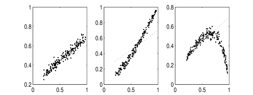
Figure 2: Simulated proportions of voters for party 1 in the first (X) and the second (Y) election for no confounding, concordant and discordant effects; dashed line is the expected relation under no confounding.

Under the discordant model and the settings described above, 1000 samples were generated and, for each sample, the maximum likelihood estimates under the correct model were computed. To see how the properties of the estimates changed with the sample size, estimates were computed also for the case where the number of voters per polling stations were between 2400 and 3200. Estimates of the bias on each parameter are given in Table 1 below: they are small and seem to decrease with sample size. Only for the overdispersion parameter, the bias is a little more substantial. Ratios between the average standard errors of the estimates computed from the information matrix and those estimated from the sample variances are given in the same table: the fact that the ratios are smaller than 1 indicates that standard errors computed from the information matrix underestimate slightly sample variability and the effect decreases with the sample size. Again the performance is worst relative to $\tau$.

Table 1: Sample bias and ratios of standard errors based on information matrix and sample variances

Sample size		$\alpha_{11}$	$\alpha_{21}$	$\tau$	$\beta_{11}$	$\beta_{21}$
600-800	Bias	-0.0202	0.0312	-0.1006	0.0054	0.0118
2400-3200	Bias	-0.0038	0.0069	-0.0744	0.0011	0.0028
600-800	Ratios of s.e.	0.9654	0.9616	0.9140	0.9656	0.9641
2400-3200	Ratios of s.e.	0.9943	0.9985	0.9330	0.9939	0.9906

The proportion of sample estimates with an absolute error that exceeds given thresholds taken from the normal distribution are displayed in Table 2: when the sample size is smaller the distribution of the sample estimates for most parameters appear to have heavier tails relative to the normal.

Table 2: Proportion of sample estimates whose absolute error exceeds $z\hat{\sigma}$

$z$	1.2815	1.6449	1.9600	2.576		1.2815	1.6449	1.9600	2.576
$\alpha_{11}$	0.1660	0.0960	0.0500	0.0200		0.1960	0.0920	0.0470	0.0140
$\alpha_{21}$	0.1780	0.1040	0.0510	0.0150		0.2010	0.0910	0.0490	0.0120
$\tau$	0.1890	0.1090	0.0540	0.0140		0.1860	0.1020	0.0570	0.0160
$\beta_{11}$	0.1800	0.0850	0.0540	0.0190		0.1880	0.0920	0.0450	0.0100
$\alpha_{21}$	0.1950	0.1070	0.0560	0.0140		0.1950	0.0980	0.0490	0.0160

4 An application

In May 15th 2011 in the city of Milan there was an election for the mayor and party representatives in the city council followed on the 29th by a run-off ballot between the previous mayor Mrs Moratti supported by the Mr Berlusconi’s gouverning coalition and Mr Pisapia supported by most parties from the left. A national referendum promoted by the opposition party Italia dei Valori (IdV) was held on June 12th to cancel several laws passed by the gouvernment. One of these laws allowed the Prime Minister, who is under trial under several accusations, to claim that the duties of his office prevented him from attending the Courts, thus postponing a decision at his will. In this application we study the behaviour of voters at the Referendum on this particular issue relative to their behaviour at the run-off ballot: Berlusconi and his supporters had campaigned for not going to vote at the referendum because, if less than 50% went to vote, the result of the referendum would be irrelevant. Lega Nord (LN), which belongs to the gouverning coalition, was much less motivated in supporting Berlusconi on this specific issue relative to voters of Partito delle Liberta’ (PdL), Berlusconi’s own party. It is likely that some of the supporters of the center opposition party Unione di Centro (UdC), who abstained at the run-off feeling that Pisapia was much to the left, decided to vote with the left parties at the referendum.

The municipality of Milan has about 990 thousands voters; after excluding the few atypical polling stations like hospitals, we could use data from 1159 polling stations. As covariates we used the centered logits of the proportion of votes cast on May 15the for the following options: (i) Pdl, (ii) (LN), (iii) UdC, (iv) (IdV), (v) abstain and blank ballots (NoV). The estimated transition matrix with standard errors, averaged across polling stations, are given on the left-hand side of Table 3 and the estimated effects of covariates are on the right-hand side of the same table. As expected, a large proportion of those who supported Pisapia voted ”yes” at the Referendum which was also supported by almost 30% of voters who had abstained at the run-off. Even more interesting is that over 22% of those who had supported Moratti did not follow Berlusconi’s recommendations and went to vote at the Referendum, Estimates of the regression parameters, which are all highly significant is briefly discussed below. Note that, whenever we assume that a covariate affects the residual category of NoV, the actual sign of the regression parameter which is estimated from the induced effect on the other voting options, is reversed.

Table 3: Average estimated transitions from Ballot to Referendum and covariates effects

Transition Probabilities					Regression estimates
	Yes	No	NoV		Covariate	$\hat{\beta}$	s.e.($\beta$)
Moratti	0.1388	0.0858	0.7754		LN on Yes $\mid$ Moratti	0,3311	0,1061
s.s.	0.0208	0.0068	0.0219		UdC on Yes$\mid$ Pisapia	0.0810	0,0282
Pisapia	0.9380	0.0000	0.0620		NoV on Yes-No $\mid$ NoV	-0.7326	0,0692
s.e.	0.0140	0.0000	0.0140		PdL on Yes-No $\mid$ Moratti	-0.3996	0,0637
NoV	0.2938	0.0428	0.6633		IdV on Yes-No $\mid$ Pisapia	0.4167	0.078
s.e.	0.0211	0.0061	0.0223

• the proportion of those who voted ”yes” at the Referendum, having supported Moratti at the Ballot, increases in polling stations with a larger proportion of voters for LN; this indicates that these voters were reluctant to follow Berlusconi on this issue;

• the proportion of those who abstained at the Referendum, having supported Moratti at the Ballot, increased in polling stations with a larger proportion of voters for PdL; this indicates that PdL supporters tended to obey the recommendation of their party;

• the proportion of those who voted ”yes” at the Referendum, having abstained at the Ballot, increased in polling stations with a larger proportion of voters for UdC as expected;

• the proportion of those who abstained at the Referendum, having abstained at the Ballot, increased in polling stations with a larger proportion of abstainers; this indicates that there is a structural proportion of voters who abstain most of the time;

• the proportion of those who abstained at the Referendum, having supported Pisapia at the Ballot, decreased in polling stations with a larger proportion of voters for IdV; this is consistent with the fact that these voters were the most militant on the issue.

References

- Alvarez et al. (2006) Alvarez. M.R.. Boehmke F.J.. Nagler J.. 2006. Strategic voting in British elections. Electoral Studies. 25. 1–19.
- Bartolucci et al (2001) Bartolucci. F.. Forcina. A.& Dardanoni. V. (2001) Positive quandrant dependence and marginal modelling in two-way tables with ordered margins. Journal of the American Statistical Association. 96. 1497–1505.
- Brown and Payne (1986) Brown. P.& Payne. C. (1986) Aggregate data. ecological regression and voting transitions. Journal of the American Statistical Association. 81. 453–460.
- Chambers and Steel (2001) Chambers. R.L.. Steel. D.G. (2001(. Simple methods for ecological inference in tables. Journal of the Royal Statist. Soc. A. 164. 175–192.
- Firth (1982) Firth. D. (1982). Estimation of voter transition matrices from election data. PhD Thesis. Dept. of Mathematics. Imperial College. London SW7.
- Forcina and Marchetti (1989) Forcina. A.. Marchetti. G.M. (2011). Modelling transition probabilities in the analysis of aggregate data. Statistical Modelling, Decarli, A., Francis, B. J., Gilchrist, R., Seber, G. U. H. (Eds.) Springer Verlag.
- Forcina and Marchetti (2011) Forcina. A.. Marchetti. G.M. (2011). The Brown and Payne model of voter transition revisited. New Perspectives in Statistical Modelling and Data Analysis. Ingrassia. S.. Rocci. R. and Vichi. M. (Eds.). 481–488. Springer. Heidelberg.
- Gelman et al (2001) Gelman. A.. Park. D.K.. Ansolabehere. S.. Price. P.N.. Minnite. L.C. (2001). Models. assumptions and model checking in ecological regressions. Journal of the Royal Statist. Soc. A. 164. 101–118
- Glynn and Wakefield (2010) Glynn. A.N. and Wakefield. J. (2001). Ecological inference in the social sciences. Statistical Methodology. 7. 307–322
- Goodman (1953) Goodman. L. A.. (1953). Ecological regression and the behaviour of individuals. American Sociological Review. 18. 351–367.
- Greiner and Quinn (2009) Greiner. D.J.. Quinn. K.M. (2009). ecological inference: bounds. correlations. flexibility and transparency of assumptions. Journal of the Royal Statist. Soc. A. 172. 67–81.
- Guthrie and Sheppard (2001) Guthrie. K.A.. Sheppard. L. (2001(. Overcoming biases and misconceptions in ecological studies. Journal of the Royal Statist. Soc. A. 164. 141–154.
- King (1997) King. G.. (1997). A Solution to the Ecological Inference Problem: Reconstructing Individual Behavior from Aggregate Data. Princeton University Press. Princeton. NJ.
- King et al. (1999) King. G.. Rosen. O. and Tanner. M. A.. (1999). Binomial-Beta Hierarchical Models for Ecological Inference. Sociological Methods & Research. 28. 61–30.
- King et al. (2004) King. G.. Rosen. O. and Tanner. M. A.. Eds. (2004). Ecological inference. Cambridge University Press. Cambridge.
- Pearl (1995) Pearl. J. (1995(. Causal diagrams for empirical research. Biometrika 82. 669–688 (1995)
- Robinson (1950) Robinson. W.S.. (1950). Ecological correlations and the behaviour of individuals. Ann. Sociol. Rev.. 15. 351–357.
- Wakefield (2004) Wakefield. J.. (2004). Ecological inference for tables. Journal of the Royal Statist. Soc. A. 167. 1–42.