Steady-State Ab Initio Laser Theory for N-level Lasers

Abstract

We show that Steady-state Ab initio Laser Theory (SALT) can be applied to find the stationary multimode lasing properties of an $N$-level laser. This is achieved by mapping the $N$-level rate equations to an effective two-level model of the type solved by the SALT algorithm. This mapping yields excellent agreement with more computationally demanding $N$-level time domain solutions for the steady state.

¹Department of Applied Physics, Yale University, New Haven, CT 06520 ²Department of Electrical Engineering, Princeton University, Princeton, NJ 08544 ^∗Corresponding author: douglas.stone@yale.edu

(140.3430) Laser Theory.

1 Introduction

Semiclassical laser theory, which neglects the quantum fluctuations of the electromagnetic field, is widely used to describe and simulate lasers [1, 2]. In principle, it correctly describes the laser thresholds and frequencies, the spatial pattern of the lasing modes, and the laser output power, including all classical non-linear effects, such as spatial hole-burning, gain saturation, and mode and phase locking. Essentially the theory describes Maxwell’s equations in an open cavity, coupled to the non-linear polarization of the gain medium. The gain polarization can be described using either a classical non-linear oscillator model [3], or a quantum-mechanical model of $N$ atomic levels in which the polarization and level populations obey the equations of motion of the quantum density matrix. The simplest version of the theory, used widely in textbooks, is the two-level Maxwell-Bloch (MB) model [1]; however, most design and characterization simulations of lasers use models with $N=3$ or more levels. In addition, most theoretical solutions for the semiclassical laser equations employ a large number of simplifying assumptions in order to make them analytically tractable, most notably neglecting the openness of the cavity and/or treating only simple one-dimensional (1D) or ring cavities, as well as approximating the non-linear interactions to cubic order. The results are typically not useful for quantitative modeling. Until recently, the only useful way to obtain quantitative results for non-trivial laser structures was to integrate the semiclassical laser equations in space and time. For novel and interesting new laser structures with non-trivial 2D and 3D cavity geometries, such simulations are at the limits of computational feasibility, making it difficult to study a large parameter space or ensemble of designs.

In the past five years a new approach to finding the stationary solutions of the semiclassical laser equations has been developed, known as Steady state Ab initio Laser Theory (SALT)[6, 7, 8, 9]. SALT treats the openness of the cavity exactly, and the multimode non-linear interactions to infinite order (with two approximations, to be discussed below). It is applicable to cavities of arbitrary complexity in 2D and 3D, although we will discuss here only the scalar wave equation coupled to a gain medium. Importantly, this approach eliminates the need to perform a time integration to steady-state, dramatically reducing the computational effort and allowing one to study cavities with high spatial complexity, such as 2D random lasers [8, 10], photonic crystal lasers [11, 12] and chaotic disk microlasers [13, 14].

SALT was originally formulated to solve the steady-state two-level Maxwell-Bloch equations [6, 7] in the standard slowly-varying envelope approximation (SVEA), and an iterative algorithm was developed [7] to solve the resulting SALT equations. Subsequently it was realized that the SVEA afforded no advantage in numerical solutions of the SALT equations, so this approximation was dropped, leading to slightly different SALT equations [14, 15], which were used in all subsequent work [8, 9, 12]. Recently an important generalization of the SALT solution algorithm was developed, improving its performance for laser cavities with complex spatial index variation and inhomogeneous pumping [9]. In its present form, SALT only employs two approximations, the stationary inversion approximation (SIA) and the rotating wave approximation (RWA), which are both well satisfied for most lasers of interest. In Ref. [15], the results of SALT were compared to the full time-dependent solution of the MB equations for a simple 1D cavity in the multimode regime, well above threshold. Excellent agreement was found in the parameter regime for which the SIA holds. This was, to our knowledge, the first demonstration of a frequency-domain method which agrees with exact time-domain methods for above-threshold multimode lasing.

Previous applications of SALT have focused on two-level gain media. In order for SALT to be a useful modeling tool, it is necessary to demonstrate that it can be applied to $N$-level lasers. In the current work, we show analytically that the steady-state equations for an $N$-level laser can be reduced to those for an effective two-level system, and hence solved using the efficient SALT algorithm with essentially the same degree of computational effort. We also explore how this effective two-level system differs from the ordinary two-level laser. Next, we present a numerical comparison between the results of SALT calculations and exact $N$-level finite-difference time-domain (FDTD) calculations, for the same simple 1D laser studied in [15], as well as for a 1D random laser. We note that a similar comparison between SALT and FDTD has been performed for a four-level high-Q single-mode photonic crystal laser in Ref. [12], with good agreement found. Here, we test SALT’s accuracy in treating the more challenging case of multimode lasing in low-Q and random cavities.

2 Effective two-level systems

2.1 Four level system analysis

We illustrate the approach using the semi-classical laser equations [1] for the four-level atomic gain medium shown in Fig. 1:

$$4\pi\ddot{\mathbf{P}}^{+} = c^{2}\nabla^{2}\mathbf{E}^{+}-\varepsilon_{c}(\mathbf{r})\ddot{\mathbf{E}}^{+}$$ (1)

$$\dot{\mathbf{P}}^{+} = -\left(i\omega_{a}+\gamma_{\perp}\right)\mathbf{P}^{+}+\frac{g^{2}}{i\hbar}\mathbf{E}^{+}\left(\rho_{22}-\rho_{11}\right)$$ (2)

$$\dot{\rho}_{33} = \mathcal{P}\left(\rho_{00}-\rho_{33}\right)-\gamma_{23}\rho_{33}$$ (3)

$$\dot{\rho}_{22} = \gamma_{23}\rho_{33}-\gamma_{12}\rho_{22}-\frac{1}{i\hbar}\mathbf{E}^{+}\cdot\left((\mathbf{P}^{+})^{*}-\mathbf{P}^{+}\right)$$ (4)

$$\dot{\rho}_{11} = \gamma_{12}\rho_{22}-\gamma_{01}\rho_{11}+\frac{1}{i\hbar}\mathbf{E}^{+}\cdot\left((\mathbf{P}^{+})^{*}-\mathbf{P}^{+}\right)$$ (5)

$$\dot{\rho}_{00} = \gamma_{01}\rho_{11}-\mathcal{P}\left(\rho_{00}-\rho_{33}\right).$$ (6)

The RWA has already been made, and we have assumed a lasing structure with one or two directions of translational symmetry, so that TM and TE polarizations are conserved and Maxwell’s equations reduce to a scalar Helmholtz equation [16]. $\mathbf{E}^{+}$ and $\mathbf{P}^{+}$ are the positive frequency components of the scalar electric and polarization fields respectively. $\rho_{ii}$ is the population density of level $|i\rangle$, $\omega_{a}$ is the frequency of the gain center, $\gamma_{\perp}$ is the gain width (polarization dephasing rate), $g$ is the dipole matrix element, $\mathcal{P}$ is the pump rate, and $\gamma_{ij}$ is the decay rate from level $|j\rangle$ to level $|i\rangle$. The four levels are labelled from $0-3$ in order of increasing energy (Fig. 1). The polarization equation (2) is obtained from the four-level density matrix equation of motion, assuming that only the level $2\to 1$ transition will be inverted and lase. Often in FDTD calculations a real classical oscillating dipole equation is used to describe the polarization [12]; in Appendix A, we show that this yields essentially the same results, with an appropriate identification of parameters. In the rate equations (3)-(6), the pump is coherently acting between levels $|0\rangle$ and $|3\rangle$.

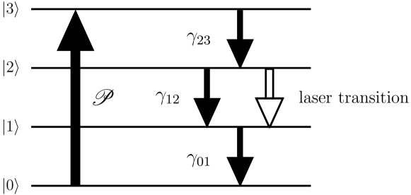
Figure 1: Schematic of a four-level gain medium.

The polarization equation (2) incorporates the inversion $D(x,t)\equiv\rho_{22}(x,t)-\rho_{11}(x,t)$, similar to the polarization equation for a two-level laser. By assuming that the non-lasing populations are stationary, $\dot{\rho}_{00}=\dot{\rho}_{33}=0$, we can show that $D(x,t)$ obeys

$$\dot{D}=-\gamma_{\parallel}^{\prime}(D-D_{0}^{\prime})-\frac{2}{i\hbar}\mathbf{E}^{+}\cdot\left((\mathbf{P}^{+})^{*}-\mathbf{P}^{+}\right),$$ (7)

which is precisely the form of the inversion equation for the two-level medium [1, 18]. The parameters $D_{0}^{\prime}$ and $\gamma_{\parallel}^{\prime}$ serve as an effective equilibrium inversion and inversion relaxation rate respectively, and are given by [14]:

$$\gamma_{\parallel}^{\prime} = 2\gamma_{12}\left(1+\frac{S}{2+\frac{\gamma_{01}}{\mathcal{P}}+2\frac{\gamma_{01}}{\gamma_{23}}}\right)$$ (8)

$$D_{0}^{\prime} = \frac{S\mathcal{P}\,n}{\gamma_{01}+\left(S+2+2\frac{\gamma_{01}}{\gamma_{23}}\right)\mathcal{P}},$$ (9)

where $S=(\gamma_{01}-\gamma_{12})/\gamma_{12}$ and $n=\sum_{i}\rho_{ii}$ is the total density of gain atoms. Eq. (9) for the inversion in the absence of laser emission (which here acts as the effective pump parameter) has been discussed by Siegman [3], while Eq. (8) for the effective relaxation rate has been derived for a special case by Khanin [19]. These expressions have not been used previously to solve the four-level lasing equations in terms of the two-level solutions, as we do here. If we use an incoherent pump, the $\mathcal{P}(\rho_{00}-\rho_{33})$ terms in (3) and (6) would be replaced by $\mathcal{P}\rho_{00}$; the effect of this would be the removal of the factor of $2$ preceding the ratio $\gamma_{01}/\gamma_{23}$ in the denominators of (8) and (9). For typical laser systems, each denominator is dominated by the $\gamma_{01}/\mathcal{P}$ term, so the difference between coherently and incoherently pumping the system is negligible [17].

Given the parameters $\{\gamma_{01},\gamma_{12},\gamma_{23},\mathcal{P}\}$ describing the four-level medium of Fig. 2, we can calculate the effective pump and relaxation rates, and feed those (together with the cavity dielectric function, lasing transition frequency $\omega_{a}$, and gain linewidth $\gamma_{\perp}$) into the SALT algorithm. That will yield the steady-state lasing properties of this four-level laser.

2.2 Arbitrary number of levels

A general $N$-level laser can be treated via an analogous procedure. Suppose we have a gain medium with an arbitrary number of levels, $N$. We assume that there is only a single lasing transition, between two levels which we denote by $|u\rangle$ and $|l\rangle$. The population of each of the $N-2$ non-lasing levels obeys

$$\dot{\rho}_{ii}=\sum_{j}\gamma_{ij}\rho_{jj}-\sum_{j}\gamma_{ji}\rho_{ii}+\gamma_{iu}\rho_{uu}+\gamma_{il}\rho_{ll}-(\gamma_{ui}+\gamma_{li})\rho_{ii},$$ (10)

where the sums are taken over all of the non-lasing states and $\gamma_{ij}$ is the rate at which atoms transition from state $|j\rangle$ to $|i\rangle$ which is either a decay or pump rate depending on the relative energies of the states. In this way, we can incorporate decay and pump processes between any levels. We again assume that $\dot{\rho}_{ii}=0$ for all non-lasing levels. Then

$$\sum_{j}\left[(s_{i}+\gamma_{ui}+\gamma_{li})\delta_{ij}-\gamma_{ij}\right]\rho_{jj}=\gamma_{iu}\rho_{uu}+\gamma_{il}\rho_{ll},$$ (11)

where $s_{i}=\Sigma_{j}\gamma_{ji}$ and $\delta_{ij}$ is the Kronecker delta. The term in brackets on the left hand side corresponds to an $(N-2)\times(N-2)$ matrix, which we denote as $R$. Upon inverting Eq. (11) and substituting it into the equations of motion for the lasing levels, we obtain

$$\gamma_{\parallel}^{\prime}=\frac{B_{l}T_{u}-B_{u}T_{l}}{T_{u}+T_{l}},\qquad\;D_{0}^{\prime}=\frac{B_{u}+B_{l}}{T_{u}+T_{l}}\;\frac{n}{\gamma_{\parallel}^{\prime}},$$ (12)

where

$$T_{u/l} = 1+\sum_{ij}[R^{-1}]_{ij}\,\gamma_{j,u/l}$$ (13)

$$B_{u} = -s_{u}+\sum_{ij}(\gamma_{ui}-\gamma_{li})[R^{-1}]_{ij}\gamma_{ju},$$ (14)

$$B_{l} = s_{l}+\sum_{ij}(\gamma_{ui}-\gamma_{li})[R^{-1}]_{ij}\gamma_{jl}.$$ (15)

The details of this calculation are given in Appendix B.

3 Physical Limits of Interest

Returning to the typical four-level case, we take note of two important physical regimes. The first, the linear regime, is $\gamma_{23}\sim\gamma_{01}\gg\gamma_{12}\gg\mathcal{P}$, for which one recovers the expected behavior that the equilibrium inversion increases linearly with the pump and that $\gamma_{\parallel}^{\prime}$ is a constant:

$$\gamma_{\parallel}^{\prime} \approx 2\gamma_{12},$$ (16)

$$D_{0}^{\prime} \approx \frac{\mathcal{P}}{\gamma_{12}}n.$$ (17)

In this case, varying the equilibrium inversion and the pump strength are essentially equivalent.

The second regime of interest, the non-linear regime, is $\gamma_{23}\sim\gamma_{01}\gg\gamma_{12}\sim\mathcal{P}$, i.e. when the slow decay rate between the lasing levels is on the same order as the pump rate. In this regime, $\gamma_{\parallel}^{\prime}$ increases with increasing pump and $D_{0}^{\prime}$ saturates with increasing pump:

$$\gamma_{\parallel}^{\prime} \approx 2\left(\gamma_{12}+\mathcal{P}\right),$$ (18)

$$D_{0}^{\prime} \approx \frac{1}{1+\frac{\mathcal{P}}{\gamma_{12}}}\left(\frac{\mathcal{P}}{\gamma_{12}}\right)n.$$ (19)

This regime is also interesting from the viewpoint of SALT. As $\gamma_{\parallel}^{\prime}$ increases with $\mathcal{P}$, a laser could satisfy the inequality $\gamma_{\parallel}^{\prime}\ll\gamma_{\perp}$ near threshold, leading to stationary inversion and an accurate solution via SALT, but fail to satisfy the inequality as the pump becomes stronger, leading to a decrease in the accuracy of SALT.

For a system with an arbitrary number of levels, the first regime always occurs at sufficiently small pump values; the second regime is obtainable if electrons in the upper lasing level are relatively long-lived compared to electrons in other levels.

4 Brief Summary of SALT

For completeness we briefly outline SALT. The $E^{+}$ and $P^{+}$ fields are assumed to obey a multi-mode ansatz

$$\begin{aligned} E^{+}(\vec{r},t)&=\sum_{\mu=1}^{M}\Psi_{\mu}(\vec{r})\,e^{-i\omega_{\mu}t},\\ P^{+}(\vec{r},t)&=\sum_{\mu=1}^{M}p_{\mu}(\vec{r})\,e^{-i\omega_{\mu}t},\end{aligned}$$ (20)

where the indices $\mu=1,2,\cdots,M$ label the different lasing modes, and the field and polarization are now explicitly scalar quantities. The total number of modes, $M$, is not given, but increases in unit steps from zero as we increase the pump strength $D_{0}$. The values of $D_{0}$ at which each step occurs are the (interacting) modal thresholds, to be determined self-consistently from the theory. The real numbers $\omega_{\mu}$ are the lasing frequencies of the modes (henceforth $c=1$), which will also be determined self-consistently.

We insert the ansatz (20) into the two-level laser equations, and employ the stationary inversion approximation (SIA) $\dot{D}=0$. The result is a set of coupled nonlinear differential equations, which are the fundamental equations of SALT [9]:

$$\left[\nabla^{2}+\left(\epsilon_{c}(\vec{r})+\frac{\gamma_{\perp}D(\vec{r})}{k_{\mu}-k_{a}+i\gamma_{\perp}}\right)k_{\mu}^{2}\right]\Psi_{\mu}(\vec{r})=0,$$ (21)

$$D(\vec{r})=D_{0}(\vec{r})\,\left[1+\sum_{\nu=1}^{M}\Gamma_{\nu}|\Psi_{\nu}(\vec{r})|^{2}\right]^{-1}.$$ (22)

$\Psi$ and $D$ are now dimensionless, measured in their natural units $E_{c}=\hbar\sqrt{\gamma_{\parallel}\gamma_{\perp}}/(2g)$ and $D_{c}=\hbar\gamma_{\perp}/(4\pi g^{2})$, and $\Gamma_{\nu}\equiv\gamma_{\perp}^{2}/(\gamma_{\perp}^{2}+(\omega_{\nu}-\omega_{a})^{2})$ is the Lorentzian gain curve evaluated at frequency $\omega_{\nu}$. Note that these equations are time-independent; Eq. (21) is a stationary wave equation for the electric field mode $\Psi_{\mu}$, with an effective dielectric function consisting of both the “passive” contribution $\epsilon_{c}(\vec{r})$ and an “active” contribution from the gain medium. The latter is frequency-dependent, and has both a real part and a negative (amplifying) imaginary part. It also includes infinite-order nonlinear “hole-burning” modal interactions, seen in the $|\Psi_{\nu}|^{2}$ dependence of (22). In addition, we make the key requirement that $\Psi_{\mu}$ must be purely out-going outside the cavity; it is this condition that makes the problem non-Hermitian. It is worth noting that the SIA is not needed until at least two modes are above threshold, so (22) is exact for single-mode lasing up to and including the second threshold (aside from the well-obeyed RWA).

These equations are solved efficiently by projecting them onto a complete biorthogonal set of purely outgoing states with external wavevectors, $k_{\mu}$, equal to the lasing frequencies. We refer to these states as the threshold constant flux (TCF) states, because one member of the basis set is always equal to the (non-interacting) threshold lasing mode, leading to very rapid convergence of the basis expansion above threshold [9]. The major computational effort in solving the SALT equations by this approach is in calculating the (linear) TCF states. The SALT solutions are obtained for successive values of the pump increasing from the first threshold; at each step, the coefficients of the lasing modes in the TCF basis are obtained using a standard non-linear solver, with the coefficients from the previous step as an initial guess (which is never far from the correct solution). Unlike FDTD, in the current version of SALT one cannot simply directly solve at a fixed pump value, well above threshold. However, even with this limitation, SALT is much more efficient, and provides substantial physical insight, as we will discuss below.

5 Numerical comparison

To perform a well-controlled comparison between SALT and the four-level laser equations (1)-(6), as well as $N$-level generalizations, we studied 1D microcavity lasers for which the FDTD calculations are tractable and fast enough to generate extensive steady-state data. We first consider the same simple edge emitting uniform-index laser treated in Refs. [6, 7, 15], with a perfect mirror at the origin, active region of length $L$ terminating abruptly in air (see schematic, Fig. 2). The simulations were carried out using standard FDTD for the electromagnetic field, and Crank-Nicholson discretization for the polarization and rate equations based on the method of Bidégaray [20] (in which the polarization and inversion are spatially aligned with the electric field but updated at the same time steps as the magnetic field). The reported modal intensities are calculated by Fourier transforming the electric field at the cavity boundary after the simulation has reached steady state (see §6 for a discussion of the steady-state criterion). The lasing transition frequency $\omega_{a}$ is chosen so that $n_{0}k_{a}L=60$, corresponding to roughly ten wavelengths of radiation within the cavity. Physical quantities are reported in terms of their natural scales, $D_{c}=\hbar\gamma_{\perp}/(4\pi g^{2})$ and $E_{c}=(\hbar/2g)\sqrt{\gamma_{\perp}\gamma_{\parallel}^{\prime}}$. In addition, we take $c=\hbar=1$ and measure rates in dimensionless units, i.e. $\gamma_{\textrm{meas}}=\gamma_{\textrm{real}}L/c$. We note that the parameters chosen accurately reflect those of real microcavities at optical frequencies [12]; the complete set of simulation parameters is given in Appendix D.

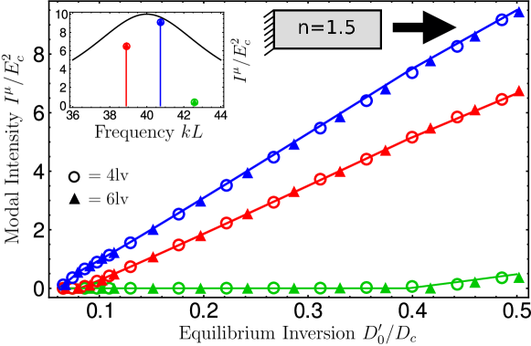
Figure 2: Modal intensities as functions of the normalized equilibrium inversion $D_{0}^{\prime}/D_{c}$ (effective pump) in a 1D microcavity edge emitting laser (schematic inset). The cavity is bounded on one side by a perfect mirror and on the other side by air, and has uniform refractive index $n=1.5$. Solid lines are results obtained by the time-independent SALT method; open circles are results of FDTD simulations with a coherently pumped four-level medium (Fig. 1); solid triangles are results of FDTD simulations with a coherently pumped six-level medium with a lasing transition between $|3\rangle$ and $|1\rangle$. Simulation parameters are given in Appendix D. Both the four-level and six-level media are chosen to satisfy SIA. The dephasing rate is $\gamma_{\perp}=4.0$. The four-level system is in the linear regime described by Eq. (16)-(17). The six-level system is calculated using the formula in the appendix B, but is in the non-linear regime described by Eq. (18)-(19). The spectra at $D_{0}/D_{c}=0.488$, and the gain curve, are shown in the upper left inset.

As shown in Fig. 2, we find close agreement between SALT calculations and FDTD simulations. At a representative pump strength $D_{0}^{\prime}=0.488D_{c}$, the mode intensities produced by SALT differ from those of the four- and six-level FDTD simulations by $\sim 1\%$, while the frequencies differ by $<0.1\%$. The difference in mode frequencies between SALT and FDTD also exists at the first lasing threshold, for which an analytical value can be calculated. There, we find that the FDTD simulation has a $0.2\%$ error in the first mode frequency, while SALT has a $0.08\%$ error; this error arises from the spatial discretization of the cavity employed in both approaches [21]. It is worth emphasizing that SALT treats the non-linearity to infinite order; in the earlier work on the Maxwell-Bloch model [15] it was shown that for this same cavity the common cubic approximation for the non-linearity fails both quantitatively and qualitatively.

These results demonstrate that so long as the system satisfies SIA, the mapping between systems with an arbitrary number of levels to an effective two-level system is nearly exact, and SALT is able to very accurately determine the steady state properties of the cavity. If two cavities, each with an arbitrary number of levels, have the same effective parameters $D_{0}^{\prime}$ and $\gamma_{\parallel}^{\prime}$, and otherwise have the same polarization relaxation rate and atomic transition frequency, the cavities are equivalent from the electromagnetic point of view, and will have identical lasing properties.

The six-level simulations shown in Fig. 2 occupy the non-linear parameter regime of Eq. (18)-(19), i.e. $\gamma_{\parallel}^{\prime}$ is a linear function and $D_{0}^{\prime}$ a non-linear function of $\mathcal{P}$. However, the unscaled modal intensity leaving the cavity is still, to leading order, linear in $\mathcal{P}$. This can be seen by rearranging (22), inserting the expressions for $\gamma_{\parallel}^{\prime}$ and $D_{0}^{\prime}$, and noting that at the end of the cavity the inversion is roughly independent of the pump strength. This result is discussed further in Appendix C.

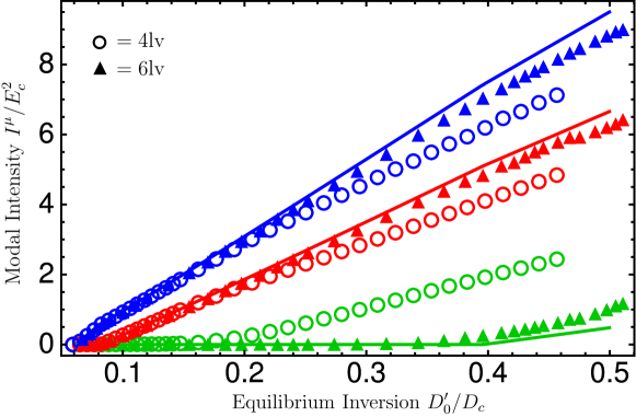
Figure 3: Breakdown of the equivalence between SALT and FDTD when SIA is not valid is shown here in two different ways. Here, modal intensities as a function of the normalized equilibrium inversion $D_{0}^{\prime}/D_{c}$ (effective pump) are shown for a 1D microcavity edge emitting laser with $\gamma_{\perp}=4.0$ and $n=1.5$. Solid lines again represent results obtained from SALT, while open circles represent FDTD simulations of a simple four-level system with $\gamma_{\parallel}^{\prime}=0.1$. Triangles represent FDTD simulations of a six-level system in the non-linear parameter regime in which $\gamma_{\parallel}^{\prime}\sim 0.001$ for $D_{0}^{\prime}\leq 0.1$, and thus satisfying SIA, but $\gamma_{\parallel}^{\prime}\sim 0.01$ for $D_{0}^{\prime}\geq 0.45$, and consequently no longer satisfying SIA.

The mapping between the $N$-level laser and two-level SALT breaks down at large pump strengths, when the condition $\gamma_{\parallel}^{\prime}\ll\gamma_{\perp}$ is violated due to the increase of $\gamma_{\parallel}^{\prime}$ with $\mathcal{P}$. In Ref. [15], following an argument by Haken [18], it was demonstrated that violating this condition causes the SIA for the two-level model to break down. This effect can be seen in the four-level laser data in Fig. 3, where $\gamma_{\parallel}^{\prime}=0.1,\gamma_{\perp}=4.0$ and accuracy is already lost for the third lasing mode. For the six-level data of Fig. 3, which is in the non-linear parameter regime, SIA is satisfied and SALT agrees with the FDTD simulations for small values of the normalized equilibrium inversion; for larger values of $D_{0}^{\prime}$, the SALT and FDTD results begin to diverge.

Finally, to demonstrate that the mapping to an effective two-level model works equally well for a complex laser cavity, Fig. 4 shows a comparison between SALT and FDTD simulations for a four-level gain medium in a 1D random dielectric structure. A number of studies have been published on random lasers using such simulations [22, 23]; SALT provides a much more efficient method for such studies, which often require generating a statistical ensemble of lasers. Here, the passive cavity dielectric function contains $\sim 31$ layers, alternating randomly between regions with refractive indices $n_{1}=1.25$ and $n_{2}=1$. Each random layer was generated according to the formula $d_{1,2}=\langle d_{1,2}\rangle(1+\eta\zeta)$ where $\langle d_{1}\rangle=(1/3)(L/30)$ and $\langle d_{2}\rangle=(2/3)(L/30)$ are the average thicknesses of the layers, $\eta=0.9$ represents the degree of randomness of the cavity, and $\zeta\in[-1,1]$ is a randomly generated number. The gain medium was added uniformly to the entire cavity, and the coherent pump was likewise uniform. The transition frequency was chosen such that $n_{1}k_{a}L=120$, corresponding to roughly $20$ wavelengths inside of the cavity. We find only small discrepancies between the SALT and FDTD results, with $\sim 1.1\%$ difference in the modal intensities. These differences did not vary significantly between different realizations of the random laser.

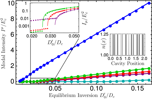
Figure 4: SALT and FDTD results for a 1D random laser. Modal intensities are plotted against the normalized equilibrium inversion $D_{0}^{\prime}/D_{c}$ (effective pump). Solid lines represent SALT results, and circles represent FDTD simulations for a four-level system with $\gamma_{\parallel}^{\prime}=0.001$. The refractive index distribution of the edge emitting random laser is described in the text. The gain medium has $\gamma_{\perp}=4.0$ and is in the regime described by Eq. (16)-(17). Left inset: log-log plot of the indicated region where three modes turn on in close proximity. Right inset: schematic of the cavity structure.

6 Computational efficiency of SALT for N-level systems

In this section we present a set of benchmarks comparing the computational efficiency of SALT to FDTD. SALT calculations enjoy three main advantages over FDTD simulations of the semiclassical laser equations. First and foremost, SALT directly finds the steady-state solutions, so no time integration is involved, which substantially decreases computational effort. Second, SALT unambiguously determines how many modes are lasing at a given pump, whereas it can be difficult to determine, especially for multimode lasing, when an FDTD simulation has reached the steady-state with all modes that will lase “on”. Third, within SALT, with minimal additional computational effort, it is possible to monitor modes which are below threshold via a modified threshold matrix [8], and hence to ascertain if more modes are likely to turn on in some interval of pump. It is important to note that the implementation of SALT used in this study has also not yet been fully optimized. For instance, the implementation of SALT used in this study requires calculating the entire lasing intensity and frequency spectrum starting from the first lasing threshold. However, this is not necessary and it is possible to implement SALT to take an initial guess of the number of modes and their relative intensities and then allow the algorithm to flow to the correct solution as the SALT algorithm has been demonstrated to be rather robust [14]. Thus, while one might assume from Fig. 5 that there would be a crossover pump value, high above threshold, where it would be more efficient to calculate the steady-state solutions using FDTD, this is not necessarily the case.

SALT does have one disadvantage that FDTD does not, assuming the cavity is not in the chaotic regime. The convergence time in FDTD is determined by the longest time scale in the problem, which is the greater of beating period between consecutive modes and the relaxation oscillation time. These time scales are relatively independent of the number of modes lasing in the cavity, so the efficiency is largely independent of the pump in the multimode regime. This is not the case for SALT, as the computational time increases as $N^{2}$ where $N$ is the number of lasing modes. However, as we see in Fig. 5, even a non-optimal implementation of SALT is substantially more efficient than FDTD even when calculating the steady state of a single pump value.

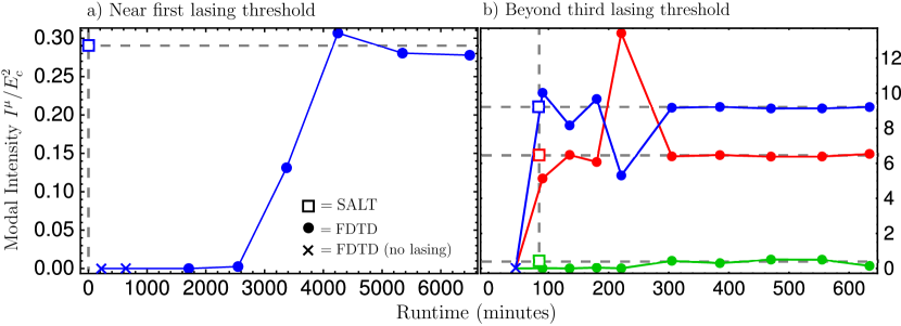
Figure 5: Comparison of SALT and FDTD run-times. Modal intensities are shown as a function of the run-time for SALT (squares) and four-level FDTD simulations (circles), using the parameters of Fig. 2. FDTD simulations that have not begun to lase are marked as crosses. Plot (a) shows data for $D_{0}/D_{c}=0.071$, just above the first lasing threshold. SALT determined the steady-state single modal intensity in under three minutes, while the FDTD required $\sim 5000$ minutes to reach steady state. Plot (b) shows data for $D_{0}/D_{c}=0.486$, well above the third lasing threshold. SALT calculated all data up to and including this pump value in under 90 minutes, whereas FDTD required $>500$ minutes for the first two modes to reach steady-state, with the third mode intensity (green circles) still fluctuating after $5000$ minutes (not shown).

Calculating full modal intensity/frequency curves as a function of the pump strength, such as in Fig. 2, is generally much more efficient using SALT. For example, in order to generate the curves seen in Fig. 2, SALT ran for a little under 2 processor hours. To generate all of the FDTD data for the four level simulations took 267 processor days. If one is attempting to explore a large parameter space of designs or system parameters, SALT may make studies feasible which are simply impractical using FDTD, particularly in more realistic 2D and 3D structures.

As mentioned before, the bulk of the computational effort required for the SALT algorithm, especially in higher dimensions, is in solving for the TCF states. While the difficulty of solving for the TCF states does scale with the dimensionality of the system, one only need solve the associated generalized eigenvalue problem $\sim 100$ (even in higher dimensions) to have a sufficiently complete basis for all pump values, whereas in FDTD one needs to solve an $O(n^{d})$ problem at each of many thousands, if not millions, of time steps. Furthermore, it is likely that switching to a finite element method in higher dimensions is not only possible, but likely to result in increased computational efficiency. Once one has a TCF basis library, using the SALT algorithm to iterate above threshold does not directly scale with the dimensionality of the system. Finally, while current implementations of SALT assume the electric field is perpendicular to the direction of wave propagation, the vectorial generalization of SALT is under investigation.

7 Conclusion

We have found that using stationarity conditions on the non-lasing level populations, the rate equations for an $N$-level laser can be mapped to an effective two-level model, for which the steady-state multimode lasing properties are efficiently solvable using Steady-state Ab initio Laser Theory (SALT). Using this mapping, we found excellent agreement between SALT and FDTD simulations for the modal frequencies, thresholds and above-threshold intensities, in the expected domain of validity. SALT is typically several orders of magnitude more efficient computationally than time domain solution of the laser-rate equations, assuming only steady-state properties are needed.

Appendix A Classical polarization in the laser-rate equations

Throughout this paper, we have used the density matrix equations of motion for the polarization field. However, much of the literature uses the classical oscillating dipole equation, in which the gain atoms are assumed to be dipoles undergoing harmonic oscillations and the quantum density matrix is neglected. This appendix briefly demonstrates that the two models are equivalent, and derives the relevant parameter redefinitions. A more thorough discussion has been given by Boyd [24].

The polarization equation used here,

$$\dot{P}^{+}=-\left(i\omega_{a}+\gamma_{\perp}\right)P^{+}+\frac{g^{2}}{i\hbar}E^{+}\left(\rho_{uu}-\rho_{ll}\right)$$ (23)

is derived from the density matrix equation

$$\dot{\rho}_{ul}=\left(i\omega_{a}+\gamma_{\perp}\right)\rho_{ul}-\frac{i}{\hbar}gE(\rho_{uu}-\rho_{ll})$$ (24)

where $|u\rangle$ and $|l\rangle$ are the upper and lower lasing states, $\rho_{ij}$ is the density matrix element $ij$ and $g_{ul}=g_{lu}=g$ is the coupling constant of the lasing states to the electric field, which allows for the definition $P^{+}=g\rho_{ul}$. Alternatively, following the notation of Boyd [24], we could consider the equation of motion for $M=g\rho_{ul}+\textrm{c.c.}=P^{+}+P^{-}$, which is the expectation value of the dipole moment induced by the applied field, i.e. the classical oscillating dipole field. Thus

$$\dot{M}=g\dot{\rho}_{ul}+\textrm{c.c.}=\left(i\omega_{a}+\gamma_{\perp}\right)\rho_{ul}-\frac{i}{\hbar}gED+\textrm{c.c.},$$ (25)

using (24), and

$$\ddot{M}=\left(-\omega_{a}^{2}+2i\omega_{a}\gamma_{\perp}+\gamma_{\perp}^{2}\right)g\rho_{ul}-\frac{\omega_{a}}{\hbar}g^{2}ED+\textrm{c.c.}.$$ (26)

This can be rewritten as

$$\ddot{M}+2\gamma_{\perp}\dot{M}+\omega_{a}^{2}M=-\gamma_{\perp}^{2}M-\frac{2\omega_{a}g^{2}}{\hbar}ED,$$ (27)

where $D=\rho_{uu}-\rho_{ll}$ is the inversion density of the lasing states. For $\omega_{a}^{2}\gg\gamma_{\perp}^{2}$, we can discard the term $\gamma_{\perp}^{2}M$, resulting in the traditional form of the classical oscillating dipole polarization field equation. This gives the classical coupling constant $\sigma=2\omega_{a}g^{2}/\hbar$ [3].

A similar analysis can used to show that the inversion equation can be rewritten as

$$\dot{D}=-\gamma_{\parallel}(D-D_{0})+\frac{2E}{\hbar\omega_{a}}\dot{M},$$ (28)

which demonstrates how the change in the inversion is dependent upon the classical polarization field. Therefore, so long as $\omega_{a}^{2}\gg\gamma_{\perp}^{2}$, a condition that is usually satisfied, these two formulations of the polarization dynamics are equivalent.

Appendix B Effective two-level parameters from N-level rate equations

This appendix derives the effective equilibrium inversion and relaxation rate for a gain medium with an arbitrary number of levels. We allow decays between any two levels, even if they are not adjacent. We assume there is a single lasing transition, between levels $|u\rangle$ and $|l\rangle$, which need not be adjacent. The rate equation for an arbitrary non-lasing level in the system is

$$\dot{\rho}_{ii}=\sum_{j}\gamma_{ij}\rho_{jj}-\sum_{j}\gamma_{ji}\rho_{ii}+\gamma_{iu}\rho_{uu}+\gamma_{il}\rho_{ll}-(\gamma_{ui}+\gamma_{li})\rho_{ii},$$ (29)

where the summations are taken over all non-lasing levels. Here we do not distinguish between decay rates and pumping rates; $\gamma_{ij}$ is simply interpreted as the rate at which level $|j\rangle$ transitions into level $|i\rangle$, regardless of the energies of those states. If the populations of all the non-lasing transitions are stationary, i.e. $\dot{\rho}_{ii}=0$, then we can rewrite (29) as

$$\sum_{j}R_{ij}\rho_{jj} = \gamma_{iu}\rho_{uu}+\gamma_{il}\rho_{ll},$$ (30)

$$R_{ij} \equiv (s_{i}+\gamma_{ui}+\gamma_{li})\delta_{ij}-\gamma_{ij}.$$ (31)

Here, $s_{i}\equiv\Sigma_{j}\gamma_{ji}$ and $\delta_{ij}$ is the Kronecker delta. Inverting (30) gives

$$\rho_{ii}=\sum_{j}[R^{-1}]_{ij}(\gamma_{ju}\rho_{uu}+\gamma_{jl}\rho_{ll}).$$ (32)

Hence, we can express the total number density of gain atoms as

$$n = \sum_{i}\rho_{ii}+\rho_{uu}+\rho_{ll}$$ (33)

$$= T_{u}\rho_{uu}+T_{l}\rho_{ll}$$ (34)

where

$$T_{u} = 1+\sum_{ij}[R^{-1}]_{ij}\gamma_{ju},$$ (35)

$$T_{l} = 1+\sum_{ij}[R^{-1}]_{ij}\gamma_{jl}.$$ (36)

Noting that $D=\rho_{uu}-\rho_{ll}$, we can write the populations of the lasing states as

$$\rho_{uu} = \frac{n+T_{l}D}{T_{l}+T_{u}},$$ (37)

$$\rho_{ll} = \frac{n-T_{u}D}{T_{l}+T_{u}}.$$ (38)

From the equations of motion for the lasing levels, we have the inversion equation

$$\dot{D}=\dot{\rho}_{uu}-\dot{\rho}_{ll}=\sum_{i}(\gamma_{ui}-\gamma_{li})\rho_{ii}-s_{u}\rho_{uu}+s_{l}\rho_{ll}-\frac{2}{i\hbar}\mathbf{E}^{+}\cdot\left((\mathbf{P}^{+})^{*}-\mathbf{P}^{+}\right),$$ (39)

where $s_{u}=\Sigma_{j}\gamma_{ju}+\gamma_{lu}$ and $s_{l}$ is defined similarly. Inserting (32) into this equation gives

$$\dot{D}=B_{u}\rho_{u,u}+B_{l}\rho_{l,l}-\frac{2}{i\hbar}\mathbf{E}^{+}\cdot\left((\mathbf{P}^{+})^{*}-\mathbf{P}^{+}\right),$$ (40)

where

$$B_{u} \equiv -s_{u}+\sum_{ij}(\gamma_{ui}-\gamma_{li})[R^{-1}]_{ij}\gamma_{ju},$$ (41)

$$B_{l} \equiv s_{l}+\sum_{ij}(\gamma_{ui}-\gamma_{li})[R^{-1}]_{ij}\gamma_{jl}.$$ (42)

Plugging in (37) and (38) now yields the inversion equation in the desired form (7), with

$$\gamma_{\parallel}^{\prime} = \frac{B_{l}T_{u}-B_{u}T_{l}}{T_{u}+T_{l}},$$ (43)

$$D_{0}^{\prime} = \frac{B_{u}+B_{l}}{B_{l}T_{u}-B_{u}T_{l}}n.$$ (44)

Appendix C Inversion as a function of the pump

In this appendix we discuss the surprising result that the unscaled modal intensities of the six-level simulations discussed in Fig. 2 as a function of the pump are approximately linear, as shown in Fig. 6, even though these six-level simulations are in the non-linear parameter regime. In simple treatments of lasers [3] the inversion is assumed to be clamped after the first lasing threshold. However, a more detailed analysis lead to the inclusion of spatial hole-burning effects which forces the inversion in the cavity to change beyond the first lasing threshold in a non-linear manner. This result then, that the unscaled modal intensity is linear in the pump rate, can be understood from the observation that at the end of the cavity, $\vec{r}=L$, all of the lasing modes have a maximum in their fields, and thus the inversion is effectively clamped at this point beyond the first lasing threshold, which can be seen in Fig. 6 (b).

To understand this formally, we begin by rewriting (22) and removing the scaling factors $E_{c}$ and $D_{c}$ gives

$$\frac{2g^{2}}{\hbar^{2}}\sum_{\nu=1}^{N}\Gamma_{\nu}|\Psi_{\nu}(\vec{r})|^{2}=\gamma_{\parallel}^{\prime}\left(\frac{D_{0}^{\prime}}{D(\vec{r})}-1\right).$$ (45)

Substituting in (18) and (19), which are valid for this simulation, gives

$$\frac{g^{2}}{\hbar^{2}}\sum_{\nu=1}^{N}\Gamma_{\nu}|\Psi_{\nu}(\vec{r})|^{2}=\mathcal{P}\left(\frac{N}{D(\vec{r})}-1\right)-\gamma_{12}.$$ (46)

The inversion $D$ is a function of both position and the pump. However, for $\vec{r}=L$ corresponding to the cavity edge, $D$ should be mostly independent of the pump, as at this location every mode is at its maximum intensity and the effect of spatial hole-burning is most pronounced. The FDTD simulation results, shown in Fig. 6, demonstrate that $D$ indeed varies very weakly with $\mathcal{P}$ at the cavity edge.

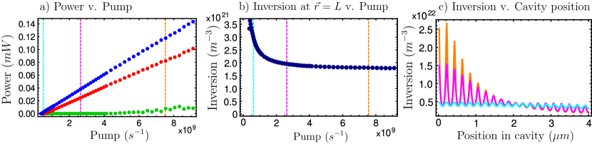
Figure 6: (a) Unscaled modal intensity of the six-level simulations from Fig. 2 as a function of the pump. A cross sectional area of $1\textrm{m}^{2}$ is assumed to calculate the power. (b) Inversion as a function of the pump at the cavity boundary. Dashed lines in plots a and b correspond to the pump values shown in plot c. (c) Inversion as a function of position within the cavity for three different pump values, cyan corresponds with $\mathcal{P}=3.75\times 10^{8}s^{-1}$, magenta with $\mathcal{P}=1.65\times 10^{9}s^{-1}$, and orange with $\mathcal{P}=4.85\times 10^{9}s^{-1}$ to show the evolution of the inversion within the cavity as a function of the pump strength.

Appendix D Simulation constants

In this appendix we list the parameters used in each of the FDTD simulations described above. These constants are matrices, with $\gamma_{ij}$ denoting the decay rate from $|j\rangle$ to $|i\rangle$. These values are given in their dimensionless form, i.e. $\gamma_{\textrm{meas}}=\gamma_{\textrm{real}}L/c$. Unlisted entries are zero. We also note that throughout this paper $|0\rangle$ denotes the ground state, so these matrices are $0$ indexed.

For the four-level simulations in Fig. 2,

$$\gamma_{4\textrm{lv, fig \ref{fig1}}}=\left(\begin{array}[]{cccc}\cdot&0.8&\cdot&\cdot\\ \cdot&\cdot&5\times 10^{-4}&\cdot\\ \cdot&\cdot&\cdot&0.8\\ \cdot&\cdot&\cdot&\cdot\\ \end{array}\right).$$ (47)

The dipole matrix element is $g=2.3\cdot 10^{-12}\textrm{m}^{3/2}$, and the number of gain atoms is $n=5\cdot 10^{23}\textrm{m}^{-3}$. The pump $\mathcal{P}$ was varied between $3\cdot 10^{-6}$ and $3\cdot 10^{-5}$.

Thus, for an optical wavelength of $\lambda=628\textrm{nm}$, the requirement in Fig. 2 that $n_{0}kL=60$ means that $L=4\mu\textrm{m}$. Using this length, the decay rates can be converted to their unit-full values as $\gamma_{\perp}=3\cdot 10^{14}\textrm{s}^{-1}$, $\gamma_{23}=\gamma_{01}=6\cdot 10^{13}\textrm{s}^{-1}$, $\gamma_{12}=3.75\cdot 10^{10}\textrm{s}^{-1}$, and the pump at threshold is $\mathcal{P}=3\cdot 10^{8}\textrm{s}^{-1}$. Similarly, the dipole matrix element also acquires units of inverse time, and can be expressed as $g^{2}/\hbar=3.98\cdot 10^{-9}\textrm{m}^{3}/\textrm{s}$, which corresponds to a coupling constant in the classical oscillating dipole picture of $\sigma=10^{-4}\textrm{C}^{2}/\textrm{kg}$. These constants can be seen to be similar to those used in other studies of optical microcavities [4, 12].

For the six-level simulations in Fig. 2,

$$\gamma_{6\textrm{lv, fig \ref{fig1}}}=\left(\begin{array}[]{cccccc}\cdot&0.8&10^{-5}&10^{-5}&10^{-5}&10^{-5}\\ \cdot&\cdot&0.8&10^{-5}&10^{-5}&10^{-4}\\ \cdot&\cdot&\cdot&5\times 10^{-5}&10^{-5}&10^{-5}\\ \cdot&\cdot&\cdot&\cdot&0.8&10^{-5}\\ \cdot&\cdot&\cdot&\cdot&\cdot&0.8\\ \cdot&\cdot&\cdot&\cdot&\cdot&\cdot\\ \end{array}\right).$$ (48)

Furthermore, $\gamma_{15}=10^{-4}$, and the lasing transition is between levels $|3\rangle$ and $|1\rangle$ (where the ground state is again $|0\rangle$ and the states are numbered in order of increasing energy).

For the four-level simulations in Fig. 3,

$$\gamma_{4\textrm{lv, fig \ref{fig2}}}=\left(\begin{array}[]{cccc}\cdot&0.8&\cdot&\cdot\\ \cdot&\cdot&5\times 10^{-2}&\cdot\\ \cdot&\cdot&\cdot&0.8\\ \cdot&\cdot&\cdot&\cdot\\ \end{array}\right).$$ (49)

For the six-level simulations in Fig. 3,

$$\gamma_{6\textrm{lv, fig \ref{fig2}}}=\left(\begin{array}[]{cccccc}\cdot&0.8&10^{-5}&10^{-5}&10^{-5}&10^{-5}\\ \cdot&\cdot&0.8&10^{-5}&10^{-5}&10^{-4}\\ \cdot&\cdot&\cdot&5\times 10^{-5}&10^{-5}&10^{-5}\\ \cdot&\cdot&\cdot&\cdot&0.8&10^{-5}\\ \cdot&\cdot&\cdot&\cdot&\cdot&0.8\\ \cdot&\cdot&\cdot&\cdot&\cdot&\cdot\\ \end{array}\right).$$ (50)

The four-level simulations of the random cavity in Fig. 4 used the same parameters as the four-level simulations in Fig. 2.

References

- [1] H. Haken, Light: Laser Dynamics Vol. 2 (North-Holland Phys. Publishing, New York, 1985).
- [2] W. E. Lamb, “Theory of an Optical Maser,” Phys. Rev. 134, A1429 (1964).
- [3] A. E. Siegman, Lasers (University Science Books, Mill Valley - California, 1986).
- [4] A. S. Nagra and R. A. York, “FDTD analysis of wave propagation in nonlinear absorbing and gain media,” IEEE Trans. Antennas Propag. 46, 334-340 (1998).
- [5] K. S. Yee, “Numerical solution of the initial boundary value problems involving Maxwell’s equations in isotropic media,” IEEE Trans Antennas Propag. 14, 302-307 (1966).
- [6] H. E. Türeci, A. D. Stone, and B. Collier, “Self-consistent multimode lasing theory for complex or random lasing media,” Phys. Rev. A 74, 043822 (2006).
- [7] H. E. Türeci, A. D. Stone, and L. Ge, “Theory of the spatial structure of nonlinear lasing modes,” Phys. Rev. A 76, 013813 (2007).
- [8] H. E. Türeci, L. Ge, S. Rotter, and A. D. Stone, “Strong interactions in multimode random lasers,” Science 320, 643-646 (2008).
- [9] L. Ge, Y. D. Chong, and A. D. Stone, “Steady-state ab initio laser theory: generalizations and analytic results,” Phys. Rev. A 82, 063824 (2010).
- [10] H. Cao, “Review on the latest developments in random lasers with coherent feedback,” J. Phys. A 38, 10497-10535 (2005).
- [11] O. Painter, R. K. Lee, A. Scherer, A. Yariv, J. D. O’Brien, P. D. Dapkus, and I. Kim, “Two-dimensional photonic band-gap defect mode laser,” Science 284, 1819-1821 (1999).
- [12] S. Chua, Y. D. Chong, A. D. Stone, M Soljac̆ić, and J. Bravo-Abad, “Low-threshold lasing action in photonic crystal slabs enabled by Fano resonances,” Opt. Express 19, 1539 (2011).
- [13] C. Gmachl, F. Capasso, E. E. Narimanov, J. U. Nöckel, A. D. Stone, J. Faist, D. L. Sivco, and A. Y. Cho, “High-power directional emission from microlasers with chaotic resonators,” Science 280, 1556-1564 (1998).
- [14] Li Ge, Yale PhD thesis, 2010.
- [15] L. Ge, R. J. Tandy, A. D. Stone, and H. E. Türeci, “Quantitative verification of ab initio self-consistent laser theory,” Opt. Express 16, 16895 (2008).
- [16] The equations are written for the TM case, the modifications for TE are straightforward.
- [17] The observation that coherent and incoherent pumping are nearly equivalent for most systems, is invalid when the coherent pumping is supplied at a similar frequency to the atomic lasing transition and thus interactions between the lasing field and pumping field must be taken into account.
- [18] H. Fu and H. Haken, “Multifrequency operations in a short-cavity standing-wave laser,” Phys. Rev. A 43, 2446-2454 (1991).
- [19] Y. I. Khanin, Principles of Laser Dynamics (Elsevier, Amsterdam, 1995).
- [20] B. Bidégaray, “Time discretizations for Maxwell-Bloch equations,” Numer. Meth. Partial Differential Equations 19, 284-300 (2003).
- [21] For any 1D cavity which is uniformly pumped the TCF states for solving SALT can also be found using a transfer matrix method which does not require discretizing space. We use a more general TCF solver in the calculations presented here which does discretize space.
- [22] X. Jiang and C. M. Soukoulis, “Time Dependent Theory for Random Lasers,” Phys. Rev. Lett. 85, 70 (2000).
- [23] X. Jiang, S. Feng, C. M. Soukoulis, J. Zi, J. D. Joannopoulos, and H. Cao, “Coupling, competition, and stability of modes in random lasers,” Phys. Rev. B 69, 104202 (2004).
- [24] R. W. Boyd, Nonlinear Optics (Academic Press, New York, 2008).