Roundoff errors in the problem of computing Cauchy principal value integrals

Abstract

We investigate the possibility of fast, accurate and reliable computation of the Cauchy principal value integrals $\mathchoice{{\vbox{\hbox{$\textstyle-$ }}\kern-7.7027pt}}{{\vbox{\hbox{$\scriptstyle-$ }}\kern-5.80164pt}}{{\vbox{\hbox{$\scriptscriptstyle-$ }}\kern-4.67079pt}}{{\vbox{\hbox{$\scriptscriptstyle-$ }}\kern-4.17912pt}}\!\int_{a\vphantom{{}_{0}}}^{b}f(x)(x-\tau)^{-1}dx$ $(a<\tau<b)$ using standard adaptive quadratures. In order to properly control the error tolerance for the adaptive quadrature and to obtain a reliable estimation of the approximation error, we research the possible influence of round-off errors on the computed result. As the numerical experiments confirm, the proposed method can successfully compete with other algorithms for computing such type integrals. Moreover, the presented method is very easy to implement on any system equipped with a reliable adaptive integration subroutine.
Keywords: Cauchy principal value integral, finite Hilbert transform, numerical integration, adaptive quadrature, round-off errors, Maple, Matlab
Mathematics Subject Classification: 65D30, 30E20

1 Introduction

We consider the problem of numerical evaluation of the Cauchy principal value integral

$$I_{a,b,\tau}(f)\,:=\,\mathchoice{{\vbox{\hbox{$\textstyle-$ }}\kern-7.7027pt}}{{\vbox{\hbox{$\scriptstyle-$ }}\kern-5.80164pt}}{{\vbox{\hbox{$\scriptscriptstyle-$ }}\kern-4.67079pt}}{{\vbox{\hbox{$\scriptscriptstyle-$ }}\kern-4.17912pt}}\!\int_{a}^{b}\frac{f(x)}{x-\tau}\hskip 0.86108ptdx\,=\lim\limits_{\mu\to 0^{+}}\bigg{(}\int_{a}^{\tau-\mu}+\int_{\tau+\mu}^{b}\bigg{)}\frac{f(x)}{x-\tau}\hskip 0.86108ptdx,$$ (1.1)

where $\tau\in(a,b)$, and the function $f$ has bounded first derivative. In general, the integral (1.1) exists if $f$ is Hölder continuous (cf. [3, §1.6]). The integrals of this type appear in many practical problems related to aerodynamics, wave propagation or fluid and fracture mechanics, mostly with relation to solving singular integral equations.

A great many papers devoted to the problem of numerical evaluation of the integrals of the form (1.1) have been published so far. Some of them are [4, 8, 13, 16, 17, 21]. A nice survey on the subject, along with a large number of references, is presented in [3, § 2.12.8].

Even though so many algorithms have been known for a quite long time, the subroutines for computing the integrals of the type (1.1) are not commonly available in systems for scientific computations. This is probably because most of the methods assume some properties of the function $f$, e.g. that $f$ is analytic, $f$ is smooth enough, etc. On the other hand, almost every system for scientific computations is equipped with one or more subroutines for automatic computation of the integrals

$$\int_{a}^{b}\psi(x)\hskip 0.86108ptdx\hskip 0.86108pt.$$ (1.2)

These algorithms, usually called adaptive quadratures, can compute the integrals of the form (1.2) for a very wide range of integrands.

The natural question arises: can an adaptive quadrature be successfully used to numerically compute the integral (1.1)? In this paper, we search for the positive answer to that question. Our goal is to provide tools that will allow to use an existing adaptive quadrature to compute accurate approximation to the integral (1.1), and also will help to obtain a reliable error estimation of the computed result. A usual automatic (adaptive) quadrature performs the computations until the error tolerance provided by a user (or the default, fixed one) is met. The numerical value of the Cauchy principal values integral is sometimes quite sensitive to the influence of round-off errors. If a user wishes high accuracy of the approximation, it may be difficult to select a proper error tolerance (if set too small, then the computation time may considerably increase or even the quadrature may fail to deliver reliable approximation). Thus, in the method proposed in this paper, the error tolerance is trimmed at the safe level. In particular, if the tolerance is set to zero, the algorithm is expected to compute the best (or rather near the best, within reasonable limits) possible, approximation to the integral (1.1) for given parameters $f$ and $\tau$.

The next section contains the formulation of, what may be called, the basic form of our algorithm. We apply two known analytical transformations that convert the integral (1.1) into the sum of two nonsingular integrals. In Section 3, we briefly describe the idea of adaptive quadratures. In the subsequent section, we discuss the problem of possible loss of significant digits and the influence of round-off errors on the approximation to a Cauchy principal value integral computed using the formula derived in Section 2. The obtained error estimates are crucial for the efficiency and reliability of the proposed method. As we briefly demonstrate, these estimates can be used to increase reliability of other algorithms for computing integrals of the form (1.1). In Section 5, we present many numerical examples to validate the usefulness of the proposed algorithm. The method is thoroughly tested with three different adaptive quadratures: the built-in adaptive quadrature of the Maple system, the one included in Matlab, and the one presented in [6].

2 Analytical transformations

Without loss of generality, we may restrict our attention to the case $a=-1$ and $b=1$. The computation of the Cauchy principal value integral

$$I_{\tau}(f)\,\equiv\,I_{\tau,-1,1}(f)\,=\,\mathchoice{{\vbox{\hbox{$\textstyle-$ }}\kern-7.7027pt}}{{\vbox{\hbox{$\scriptstyle-$ }}\kern-5.80164pt}}{{\vbox{\hbox{$\scriptscriptstyle-$ }}\kern-4.67079pt}}{{\vbox{\hbox{$\scriptscriptstyle-$ }}\kern-4.17912pt}}\!\int_{-1}^{1}\frac{f(x)}{x-\tau}\hskip 0.86108ptdx$$ (2.1)

may at first seem quite easy, if we observe that by a simple change of variables, setting

$$\delta=\min\{1+\tau,1-\tau\},$$ (2.2)

we obtain

$$\begin{array}[]{l}\displaystyle I{{}_{\tau}}(f)\,=\,\int_{|x-\tau|\geq\delta}\frac{f(x)}{x-\tau}\hskip 0.86108ptdx+\,\mathchoice{{\vbox{\hbox{$\textstyle-$ }}\kern-7.7027pt}}{{\vbox{\hbox{$\scriptstyle-$ }}\kern-5.80164pt}}{{\vbox{\hbox{$\scriptscriptstyle-$ }}\kern-4.67079pt}}{{\vbox{\hbox{$\scriptscriptstyle-$ }}\kern-4.17912pt}}\!\int_{\tau-\delta}^{\tau+\delta}\frac{f(x)}{x-\tau}\hskip 0.86108ptdx\\[15.0694pt] \displaystyle\hphantom{I{{}_{\tau}}(f)}\,=\,\int_{|x-\tau|\geq\delta}\frac{f(x)}{x-\tau}\hskip 0.86108ptdx+\int_{0}^{\delta}\frac{f(\tau+x)-f(\tau-x)}{x}\hskip 0.86108ptdx,\end{array}$$ (2.3)

where we use the convention that $\int_{|x-\tau|\geq\delta}\equiv\int_{\tau+\delta}^{1}$, if $\delta=1+\tau$, and $\int_{|x-\tau|\geq\delta}\equiv\int_{-1}^{\tau-\delta}$, if $\delta=1-\tau$.

The formula (2.3) was applied for the first time by Longman in [13], and it was derived by splitting the function $f$ into the odd and even parts. Both integrals on the right hand side of (2.3) exist in the Riemann sense. We should note that if the function $f$ has bounded first derivative in the neighbourhood of $\tau$, then the second integral is not even singular (unless $f$ has singularities itself).

The first integral on the right hand side of (2.3) was commonly not paid attention to, as it is always a proper one. However, if $|\tau|$ is close to $1$, then this integral is a near-singular one, and standard quadratures may fail when applied directly.

In many algorithms, another transformation of the integral $I_{\tau}(f)$ is used, usually being called subtracting out the singularity. We have

$$\begin{array}[]{l}\displaystyle I{{}_{\tau}}(f)\,=\,\mathchoice{{\vbox{\hbox{$\textstyle-$ }}\kern-7.7027pt}}{{\vbox{\hbox{$\scriptstyle-$ }}\kern-5.80164pt}}{{\vbox{\hbox{$\scriptscriptstyle-$ }}\kern-4.67079pt}}{{\vbox{\hbox{$\scriptscriptstyle-$ }}\kern-4.17912pt}}\!\int_{-1}^{1}\frac{f(\tau)}{x-\tau}\hskip 0.86108ptdx+\int_{-1}^{1}\frac{f(x)-f(\tau)}{x-\tau}\hskip 0.86108ptdx\\[13.77771pt] \displaystyle\hphantom{I{{}_{\tau}}(f)}\,=\,f(\tau)\,\log\frac{1-\tau}{1+\tau}+\int_{-1}^{1}\frac{f(x)-f(\tau)}{x-\tau}\hskip 0.86108ptdx\,.\end{array}$$ (2.4)

A direct application of the above formula is commonly not recommended (see, e.g., [8, 15]) due to possible severe cancellation, if a quadrature node happens to be very close to $\tau$.

The authors, however, have never seen the two above approaches being put together. From (2.3) and (2.4) we immediately obtain

$$I{{}_{\tau}}(f)\,=\,f(\tau)\,\log\frac{1-\tau}{1+\tau}+\int_{|x-\tau|\geq\delta}g(x)\hskip 0.86108ptdx+\int_{0}^{\delta}h(x)\hskip 0.86108ptdx,\vspace{-0.5ex}$$ (2.5)

where

$$g(x)=\frac{f(x)-f(\tau)}{x-\tau}\qquad\,\,\mathrm{and}\qquad\,\,h(x)=\frac{f(\tau+x)-f(\tau-x)}{x}.\vspace{0.3ex}$$ (2.6)

If the function $f$ has bounded first derivative, none of the integrals on the right hand side of (2.5) is singular or near-singular (unless $f$ itself has singularities just outside the interval $[-1,1]$), and, when the first integral of (2.5) is approximated numerically, the distance between $\tau$ and any of the quadrature nodes is never smaller than $\delta$.

It is clear that some loss of significance may occur when computing the values of the function $g$ and $h$ defined above. The influence of the round-off errors on the accuracy of the approximation (2.5) to the integral (2.1) is thoroughly discussed in Section 4.

3 A very short story on adaptive quadratures

The idea and basic rules of adaptive numerical integration (including some examples) is nicely presented in [3, §6] and [20, §5.2 & §5.3]. A very thorough study on the subject, together with the comprehensive history of development of adaptive quadratures, is given in [5].

In general, adaptive quadratures are meant to be able to numerically approximate the integrals of the form (1.2) for the widest possible range of integrands. The only arguments required by an adaptive algorithm are the integrand and the interval endpoints. The algorithm tries to approximate the integral with an error less than some default error tolerance or the error tolerance provided by the user. Many adaptive quadratures also report the estimation of the approximation error.

The most common idea of the adaptive integration algorithm is to split the interval of integration into subintervals of different lengths. The number of the subintervals and their lengths depend on the behaviour of the integrand, and are determined automatically during the computation process. Usually, the approximated value of the integral over a single subinterval is computed using some fixed quadrature rule. Along with the approximation, an error estimation has to be computed, e.g., by the use of another quadrature rule and comparing the results. The computations are terminated, when the estimated global error of the adaptive quadrature is less than a prescribed tolerance.

Suppose that an adaptive integration algorithm is based on the fixed linear quadrature rule

$$Q(\psi)\equiv Q(\psi,0,1)=\sum\limits_{j=0}^{m}B_{j}\hskip 0.86108pt\psi(x_{j})\quad(0\leq x_{0}<x_{1}<\dots<x_{m}\leq 1),$$ (3.1)

which approximates the integral

$$\int_{0}^{1}\psi(x)dx.$$

Then, the final approximation to the integral (1.2) computed by the adaptive quadrature is given by

$$A(\psi,a,b)=\sum\limits_{k=0}^{n-1}Q(\psi,s_{k},s_{k+1})=\sum\limits_{k=0}^{n-1}\sum\limits_{j=0}^{m}B_{kj}\hskip 0.86108pt\psi(x_{kj}),\vspace{-1ex}$$ (3.2)

where

$$B_{kj}=(s_{k+1}-s_{k})B_{j},\qquad x_{kj}=s_{k}+(s_{k+1}-s_{k})x_{j},$$

and

$$a=s_{0}<s_{1}<\dots<s_{n}=b$$

are the automatically determined endpoints of the subintervals $[s_{k},s_{k+1}]$ ($0\leq k<n$,  $n\geq 1$). The values $s_{k}$ ($0\leq k\leq n$) and the integer $n$ depend on $\psi$, $a$, $b$ and the assumed error tolerance.

If the quadrature $Q$ defined in (3.1) has the property $x_{0}=0$, $x_{m}=1$, then it is called the closed type one. If $x_{0}>0$ and $x_{m}<1$, then $Q$ is called the quadrature rule of the open type. In the similar way we shall call the related adaptive quadrature.

When computing the integrals of the form (1.2), adaptive quadratures are much more flexible compared to any fixed quadrature rule. However, it has to be noted that sometimes an adaptive algorithm may fail to compute a reliable approximation. In other words, the algorithm based on (2.5) for computing the integral (2.1) will be, in general, as reliable as the adaptive quadrature used. The problem of reliability of adaptive quadratures was thoroughly discussed in [6] and [7].

Some more information on a specific adaptive quadrature is provided in Section 5, when the given adaptive algorithm is being considered.

Computing the integrals of the form (2.1) by a simple application of the formula (2.5) may not lead to satisfactory results. The numerical values of the Cauchy principal value integrals are, in some cases, very sensitive to round-off errors. Therefore, the possible to achieve accuracy may be considerably limited, when computations are performed in a fixed precision floating point arithmetic. If we set too small error tolerance for the adaptive quadrature, the algorithm may work very long, usually being unable to reach the requested accuracy. Because of the influence of the round-off errors, the error estimation reported by the adaptive algorithm may also be false. Thus, it is very important to have some good tools that would modify the error tolerance, if necessary, and correct the error estimation computed by the adaptive quadrature.

4 Estimating round-off errors

It is quite obvious that even small changes of the values of the function $f$ near the singularity point $\tau$ may considerably change the value of the integral (2.1). Also, when using the formula (2.5), an additional error, due to the computation of values of the functions $g$ and $h$, may appear. In this section, we derive estimates of the round-off errors that will allow to control the performance of an adaptive quadrature, and will provide additional information on the accuracy of the computed approximation to the integral (2.1).

Let us denote by $\varepsilon$ the precision of the arithmetic used, and by $g^{[\varepsilon]}(x)$ and $h^{[\varepsilon]}(x)$ the numerically computed values of the functions $g$ and $h$, defined in (2.6), at the point $x$ (the argument $x$, and also the parameter $\tau$, may not have the exact representation in the floating point arithmetic). For simplicity, we will temporarily assume that the values of the function $f$ in (2.6) are computed exactly. We shall write $a\approx b$, if $a=b\big{(}1+O(\varepsilon)\big{)}$, and $a\hskip 0.86108pt\,{}^{{}_{{}_{{}_{\displaystyle{<}}}}}{}_{{}_{\displaystyle{\sim}}}\,b$, if $a<b$ or $a\approx b$.

Lemma 1.

If we define

$$D_{1,f}=\max_{|x|\leq 1}|f^{\prime}(x)|,$$ (4.1)

then for all $0<|x|\leq\delta$, where $\delta$ is defined in (2.2),

$$|h^{[\varepsilon]}(x)-h(x)|\hskip 0.86108pt\hskip 0.86108pt\,{}^{{}_{{}_{{}_{\displaystyle{<}}}}}{}_{{}_{\displaystyle{\sim}}}\,\,\frac{4\hskip 0.86108pt\varepsilon D_{1,f}}{x}+4\hskip 0.86108pt\varepsilon D_{1,f}.$$ (4.2)

Proof.

We have

$$h^{[\varepsilon]}(x)=\frac{f\big{(}(\tau(1+\gamma_{1})+x(1+\gamma_{2}))(1+\gamma_{3})\big{)}-f\big{(}(\tau(1+\gamma_{1})-x(1+\gamma_{2}))(1+\gamma_{4})\big{)}}{x(1+\gamma_{5})},$$ (4.3)

where $|\gamma_{1}|,|\gamma_{2}|,|\gamma_{3}|,|\gamma_{4}|\leq\varepsilon$ and $|\gamma_{5}|\hskip 0.86108pt\,{}^{{}_{{}_{{}_{\displaystyle{<}}}}}{}_{{}_{\displaystyle{\sim}}}\,2\varepsilon$. Further,

$$(\tau(1+\gamma_{1})+x(1+\gamma_{2}))(1+\gamma_{3})\,=\,\tau+x+\beta$$

for some $\beta$ satisfying

$$|\beta|\,\approx\,\big{|}(\gamma_{1}+\gamma_{3})\tau+(\gamma_{2}+\gamma_{3})x\big{|}\,\leq\,2\varepsilon,$$

as, by definition of $\delta$ given in (2.2), we have $|\tau|+|x|\leq 1$, if $|x|\leq\delta$. This immediately implies that

$$|f\big{(}(\tau(1+\gamma_{1})+x(1+\gamma_{2}))(1+\gamma_{3})\big{)}-f(\tau+x)|\,\leq\,|\beta|D_{1,f}\,\hskip 0.86108pt\,{}^{{}_{{}_{{}_{\displaystyle{<}}}}}{}_{{}_{\displaystyle{\sim}}}\,\,2\hskip 0.86108pt\varepsilon D_{1,f}.$$ (4.4)

Analogously,

$$|f\big{(}(\tau(1+\gamma_{1})-x(1+\gamma_{2}))(1+\gamma_{4})\big{)}-f(\tau-x)|\,\hskip 0.86108pt\,{}^{{}_{{}_{{}_{\displaystyle{<}}}}}{}_{{}_{\displaystyle{\sim}}}\,\,2\varepsilon D_{1,f}.$$ (4.5)

Now, from (4.3), (4.4) and (4.5) we obtain

$$|h^{[\varepsilon]}(x)-h(x)| \,=\,\bigg{|}h^{[\varepsilon]}(x)-\frac{\big{(}f(\tau+x)-f(\tau-x)\big{)}\hskip 0.86108pt(1+\gamma_{5})}{x(1+\gamma_{5})}\bigg{|}$$

$$\,=\,\bigg{|}h^{[\varepsilon]}(x)-\frac{f(\tau+x)-f(\tau-x)}{x(1+\gamma_{5})}-\frac{\gamma_{5}}{1+\gamma_{5}}\cdot\frac{f(\tau+x)-f(\tau-x)}{x}\bigg{|}$$

$$\,\hskip 0.86108pt\,{}^{{}_{{}_{{}_{\displaystyle{<}}}}}{}_{{}_{\displaystyle{\sim}}}\,\,\frac{4\hskip 0.86108pt\varepsilon D_{1,f}}{x}+4\hskip 0.86108pt\varepsilon D_{1,f}.$$

∎

Lemma 2.

If $|x-\tau|\geq 16\varepsilon$, then

$$|g^{[\varepsilon]}(x)-g(x)|\,\hskip 0.86108pt\,{}^{{}_{{}_{{}_{\displaystyle{<}}}}}{}_{{}_{\displaystyle{\sim}}}\,\,\frac{8\hskip 0.86108pt\varepsilon D_{1,f}}{|x-\tau|}.$$ (4.6)

Proof.

Similarly as in (4.3), we have

$$g^{[\varepsilon]}(x)=\frac{f(x(1+\gamma_{1}))-f(\tau(1+\gamma_{2}))}{(x(1+\gamma_{1})-\tau(1+\gamma_{2}))(1+\gamma_{3})},$$ (4.7)

where $|\gamma_{1}|,|\gamma_{2}|\leq\varepsilon$ and $|\gamma_{3}|\hskip 0.86108pt\,{}^{{}_{{}_{{}_{\displaystyle{<}}}}}{}_{{}_{\displaystyle{\sim}}}\,2\varepsilon$. Moreover,

$$(x(1+\gamma_{1})-\tau(1+\gamma_{2}))(1+\gamma_{3})-(x-\tau)\,=\,\beta$$ (4.8)

for some $\beta\approx x\gamma_{1}+\tau\gamma_{2}+(x-\tau)\gamma_{3}$ that satisfies

$$|\beta|\,\hskip 0.86108pt\,{}^{{}_{{}_{{}_{\displaystyle{<}}}}}{}_{{}_{\displaystyle{\sim}}}\,\,\left\{\begin{array}[]{ll}4\varepsilon\hskip 0.86108pt,&\mathrm{if}\quad|x-\tau|\leq 1,\\ 6\varepsilon\hskip 0.86108pt,&\mathrm{otherwise}.\end{array}\right.$$ (4.9)

From (4.8), we immediately obtain, that

$$(x(1+\gamma_{1})-\tau(1+\gamma_{2}))(1+\gamma_{3})\,=\,(x-\tau)\Big{(}1+\frac{\beta}{x-\tau}\Big{)}.$$ (4.10)

In addition, as $|x|,|\tau|\leq 1$, we have

$$|f(x(1+\gamma_{1}))-f(x)|\leq\varepsilon D_{1,f}\quad\mathrm{and}\quad|f(\tau(1+\gamma_{2}))-f(\tau)|\leq\varepsilon D_{1,f},$$

which, together with (4.7), (4.10), (4.9), and $|x-\tau|\geq 16\varepsilon$, gives

$$|g^{[\varepsilon]}(x)-g(x)| \,=\,\Bigg{|}g^{[\varepsilon]}(x)-\frac{f(x)-f(\tau)}{(x-\tau)\Big{(}1+\frac{\beta}{x-\tau}\Big{)}}\Big{(}1+\frac{\beta}{x-\tau}\Big{)}\Bigg{|}$$

$$\,=\,\Bigg{|}g^{[\varepsilon]}(x)-\frac{f(x)-f(\tau)}{(x-\tau)\Big{(}1+\frac{\beta}{x-\tau}\Big{)}}-\frac{\beta\,{\displaystyle\frac{f(x)-f(\tau)}{x-\tau}}}{(x-\tau)\Big{(}1+\frac{\beta}{x-\tau}\Big{)}}\Bigg{|}$$

$$\,\leq\,\frac{2\hskip 0.86108pt\varepsilon D_{1,f}+\beta D_{1,f}}{|x-\tau|\Big{(}1+\frac{\beta}{x-\tau}\Big{)}}\,\hskip 0.86108pt\,{}^{{}_{{}_{{}_{\displaystyle{<}}}}}{}_{{}_{\displaystyle{\sim}}}\,\,\frac{8\hskip 0.86108pt\varepsilon D_{1,f}}{|x-\tau|}.$$

∎

Remark 1.

The round-off error estimates of Lemmas 1 and 2 were obtained under the assumption that $D_{1,f}<\infty$, and they can allow us to derive a global round-off error estimation for the integral (2.1) computed using (2.5), which does not depend on $\tau$. It is easy to verify that the inequalities (4.2) and (4.6) could have been be replaced by more precise and much more complex estimates,

$$|h^{[\varepsilon]}(x)-h(x)|\hskip 0.86108pt\hskip 0.86108pt\,{}^{{}_{{}_{{}_{\displaystyle{<}}}}}{}_{{}_{\displaystyle{\sim}}}\,\,\frac{2\hskip 0.86108pt\varepsilon}{x}\big{(}f^{\prime}(\tau+x)+f^{\prime}(\tau-x)\big{)}\,+\,2\hskip 0.86108pt\varepsilon\big{(}\hat{f}(\tau+x,\tau)+\hat{f}(\tau-x,\tau)\big{)},$$ (4.11)

and

$$|g^{[\varepsilon]}(x)-g(x)|\,\hskip 0.86108pt\,{}^{{}_{{}_{{}_{\displaystyle{<}}}}}{}_{{}_{\displaystyle{\sim}}}\,\left\{\begin{array}[]{ll}\displaystyle\frac{4\hskip 0.86108pt\varepsilon}{3|x-\tau|}\big{(}f^{\prime}(x)+f^{\prime}(\tau)+4\hat{f}(x,\tau)\big{)},&\mathit{if}\quad|x-\tau|\leq 1,\\[10.76385pt] \displaystyle\hphantom{3}\frac{\varepsilon}{|x-\tau|}\big{(}f^{\prime}(x)+f^{\prime}(\tau)+6\hat{f}(x,\tau)\big{)},&\mathit{otherwise},\end{array}\right.\vspace{1ex}$$ (4.12)

respectively, where $\hat{f}(x,y)=(x-y)^{-1}\big{(}f(x)-f(y)\big{)}$, if, e.g., $f^{\prime\prime}$ is bounded in the $2\varepsilon$-neighbourhood of $\hskip 0.86108pt\tau$, $x$, and $\tau\pm x$. The above inequalities, however, appear to lead to no reasonably simple and usable global round-off error estimation. Therefore, in the incoming part of the paper, we shall derive uniform ($\tau$-independent) global theoretical estimates of the influence of the round-off errors, by applying (4.2) and (4.6). Still, in the implementation of the proposed method, we shall make some use of the inequalities (4.11)–(4.12).

In both lemmas we assumed that the values of the function $f$ are computed exactly. In practice, this is obviously not true. However, if the computation of $f(x)$ for every $x\in[-1,1]$ is numerically backward stable, i.e.

$$f^{[\varepsilon]}(x)=f(x(1+\gamma)),$$ (4.13)

where $f^{[\varepsilon]}(x)$ denotes the numerically computed value of $f(x)$, and $|\gamma|\leq\varepsilon K_{1}$ for some small positive $K_{1}$, then all the above results remain true, only the constant factors change. Moreover, regarding the fact that in the proofs of lemmas 1 and 2 we have bounded the errors $|\varepsilon x|$ and $|\varepsilon\tau|$ by $|\varepsilon|$ (as $|x|,|\tau|\leq 1$), we may replace (4.13) with the less restrictive condition,

$$f^{[\varepsilon]}(x)=f(x+\gamma)\qquad(-1\leq x\leq 1),$$

which better reflects the real situations, e.g., if the function $f$ depends on the shifted argument. One may suggest that it is more practical to assume that

$$f^{[\varepsilon]}(x)=f(x+\gamma)(1+\xi)\qquad(-1\leq x\leq 1),$$

where $|\xi|\leq\varepsilon K_{0}$ for some small $K_{0}>0$. In a similar manner as we have proved Lemmas 1 and 2, it can be shown that in the above case the inequalities (4.2) and (4.6) remain true, if the factor $D_{1,f}$ is replaced with

$$D_{f}\,:=\,D_{1,f}+\frac{1}{2}(K_{1}D_{1,f}+K_{0}D_{0,f}),\vspace{-0.5ex}$$ (4.14)

where

$$D_{0,f}=\max_{|x|\leq 1}|f(x)|.$$ (4.15)

4.1 The first approach – cutting of the singularity

From (4.2) and (4.6) we immediately obtain (formally) that

$$\begin{array}[]{rcl}\displaystyle E_{\varepsilon,0}(f)&:=&\displaystyle\bigg{|}\int_{|x-\tau|\geq\delta}\big{(}g^{[\varepsilon]}(x)-g(x)\big{)}\hskip 0.86108ptdx+\int_{0}^{\delta}\big{(}h^{[\varepsilon]}(x)-h(x)\big{)}\hskip 0.86108ptdx\bigg{|}\\[2.15277pt] &\leq&\displaystyle\int_{|x-\tau|\geq\delta}\big{|}g^{[\varepsilon]}(x)-g(x)\big{|}\hskip 0.86108ptdx+\int_{0}^{\delta}\big{|}h^{[\varepsilon]}(x)-h(x)\big{|}\hskip 0.86108ptdx\\[2.15277pt] &\hskip 0.86108pt\,{}^{{}_{{}_{{}_{\displaystyle{<}}}}}{}_{{}_{\displaystyle{\sim}}}&\displaystyle\int_{|x-\tau|\geq\delta}\frac{8\hskip 0.86108pt\varepsilon D_{f}}{|x-\tau|}\hskip 0.86108ptdx\,+\int_{0}^{\delta}\frac{8\hskip 0.86108pt\varepsilon D_{f}}{x}\hskip 0.86108ptdx\,\leq\,8\hskip 0.86108pt\varepsilon D_{f}\int_{-1}^{1}\frac{1}{|x-\tau|}\hskip 0.86108ptdx\,\leq\,16\hskip 0.86108pt\varepsilon D_{f}\int_{0}^{1}\frac{1}{x}\hskip 0.86108ptdx,\vspace{0.5ex}\end{array}$$ (4.16)

which may not look like a promising formula for approximating the cumulative round-off error. Thus, it seems quite natural to replace the integral $\int_{0}^{\delta}h(x)\hskip 0.86108ptdx$ in (2.5) by $\int_{\mu}^{\delta}h(x)\hskip 0.86108ptdx$ for some very small value of $\mu$ ($0<\mu\leq\delta$). In this case, we have

$$E_{\varepsilon,\mu}(f)\,\hskip 0.86108pt\,{}^{{}_{{}_{{}_{\displaystyle{<}}}}}{}_{{}_{\displaystyle{\sim}}}\,\,16\hskip 0.86108pt\varepsilon D_{f}\log(\mu^{-1})\hskip 0.86108pt.$$ (4.17)

By $A(\psi,a,b)$ we shall denote an approximated value of the integral (1.2) computed by some (adaptive) algorithm $A$. We will also define the theoretical approximation error,

$$E_{A}(\psi,a,b)=\bigg{|}\int_{a}^{b}\psi(x)\hskip 0.86108ptdx-A(\psi,a,b)\bigg{|}.$$

Now, from (2.5), (4.17), and $\big{|}\int_{0}^{\mu}h(x)\hskip 0.86108ptdx\hskip 0.86108pt\big{|}\leq 2\mu D_{1,f}$, we obtain

$$I_{\tau}(f)\hskip 0.86108pt=\hskip 0.86108ptf(\tau)\log\frac{1-\tau}{1+\tau}+A(g^{[\varepsilon]},-1,\tau-\delta)+A(g^{[\varepsilon]},\tau+\delta,1)+A(h^{[\varepsilon]},\mu,\delta)+\mathcal{E}_{1},$$ (4.18)

where

$$\begin{array}[]{rcl}\displaystyle|\mathcal{E}_{1}|&\hskip 0.86108pt\,{}^{{}_{{}_{{}_{\displaystyle{<}}}}}{}_{{}_{\displaystyle{\sim}}}&E_{A}(g^{[\varepsilon]},-1,\tau-\delta)+E_{A}(g^{[\varepsilon]},\tau+\delta,1)+E_{A}(h^{[\varepsilon]},\mu,\delta)\\ \displaystyle\hfil&+&16\hskip 0.86108pt\varepsilon D_{f}\log(\mu^{-1})+2\mu D_{1,f}.\end{array}$$ (4.19)

Because we do not design our method to be used with any particular adaptive quadrature, there is no way to know the values of the errors $E_{A}(\cdot,\cdot,\cdot)$ in advance. However, we assume that these errors will be estimated accurately enough by the adaptive algorithm itself at the time the computations are being performed.

The best value of the parameter $\mu$ in (4.19) may be determined in several ways. One could wish to minimize the error

$$\mathcal{E}_{\mu}:=16\hskip 0.86108pt\varepsilon D_{f}\log(\mu^{-1})+2\mu D_{1,f}.$$ (4.20)

Simple computations show that $\mathcal{E}_{\mu}$ reaches its minimum at $\mu=8\hskip 0.86108pt\varepsilon D_{f}D_{1,f}^{-1}$ (provided that $D_{1,f}\neq 0$). From the practical point of view, however, this value of $\mu$ is usually too small. The other reasonable, and our preferred way to determine the proper value of $\mu$ is to split the error more evenly between the last two terms of (4.19). In our implementation, we determine the value of $\mu$ as the solution of the equation

$$16\hskip 0.86108pt\varepsilon\log(\mu^{-1})=2\mu.$$ (4.21)

The above equation is satisfied for $\mu=8\hskip 0.86108pt\varepsilon W(\frac{1}{8}\varepsilon^{-1})$, where $W$ is the Lambert $W$-function (see, e.g., [2]). Subroutines for numerical evaluation of the values of the Lambert $W$-function can be found in almost every system for scientific computations. If $\varepsilon=2^{-d}$, then $8\hskip 0.86108pt\varepsilon W(\frac{1}{8}\varepsilon^{-1})\simeq(5.555d-9.747\log(d)-5.77)\varepsilon$, with the relative error less than $0.14\%$, for every $d\in\{20,21,\dots,2000\}$.

4.2 The second approach – open-type quadratures

If, for approximating the two integrals on the right hand side of (2.5), we use an adaptive quadrature of the open type, then we are guaranteed that $0$ does not belong to the set of nodes of the quadrature $A(h,0,\delta)$. Observe that, instead of (4.18), we may write

$$I_{\tau}(f)\hskip 0.86108pt=\hskip 0.86108ptf(\tau)\,\log\frac{1-\tau}{1+\tau}+A(g^{[\varepsilon]},-1,\tau-\delta)+A(g^{[\varepsilon]},\tau+\delta,1)+A(h^{[\varepsilon]},0,\delta)\hskip 0.86108pt+\hskip 0.86108pt\mathcal{E}_{2}\hskip 0.86108pt,\vspace{-0.5ex}$$ (4.22)

where

$$\begin{array}[]{rcl}\displaystyle|\mathcal{E}_{2}|&\leq&E_{A}(g,-1,\tau-\delta)+E_{A}(g,\tau+\delta,1)+E_{A}(h,0,\delta)\\ \displaystyle\hfil&+&\big{|}\tilde{A}(g^{[\varepsilon]}-g,-1,\tau-\delta)+\tilde{A}(g^{[\varepsilon]}-g,\tau+\delta,1)+\tilde{A}(h^{[\varepsilon]}-h,0,\delta)\big{|}.\end{array}$$ (4.23)

In the above inequality, the symbols $\tilde{A}(\cdot,\cdot,\cdot)$ denote the values of some (in general, arbitrary) linear quadratures of the form (3.2). For example, $\tilde{A}(g^{[\varepsilon]}-g,-1,\tau-\delta)$ is the linear combination of the form (3.2), where the subinterval endpoints $s_{k}$ were determined automatically when running the adaptive quadrature $A(g,-1,\tau-\delta)$. Now, setting

$$\mathcal{E}_{o}\hskip 0.86108pt=\hskip 0.86108pt\tilde{A}(g^{[\varepsilon]}-g,-1,\tau-\delta)+\tilde{A}(g^{[\varepsilon]}-g,\tau+\delta,1)+\tilde{A}(h^{[\varepsilon]}-h,0,\delta),\,\,$$ (4.24)

analogously to (4.16), we may obtain

$$|\mathcal{E}_{o}|\,\hskip 0.86108pt\,{}^{{}_{{}_{{}_{\displaystyle{<}}}}}{}_{{}_{\displaystyle{\sim}}}\,\,16\hskip 0.86108pt\varepsilon D_{f}\hskip 0.86108pt\tilde{A}(\frac{1}{x},0,1).\vspace{-0.5ex}$$ (4.25)

The term $\tilde{A}(x^{-1},0,1)$ is not as pessimistic as the last integral in (4.16), as it is always finite. As we shall show, the value $\tilde{A}(x^{-1},0,1)$ is not much larger than $\log(x_{00}^{-1})$, where $x_{00}$ is the smallest node of $\tilde{A}(x^{-1},0,1)$.

Without loss of generality, we may assume that the quadrature rule $Q$ defined in (3.1) satisfy the obvious condition: $\sum_{j=0}^{m}B_{j}=1$.

Lemma 3.

Assume that a quadrature $Q$ defined in (3.1) is of the open type and let $Q(\psi,a,b)$ denote the quadrature $Q$ applied (after linear transformation) to the interval $[a,b]$, i.e.

$$Q(\psi,a,b)=(b-a)\sum\limits_{j=0}^{m}B_{j}\hskip 0.86108pt\psi\big{(}a+(b-a)x_{j}\big{)}\quad(0<x_{0}<x_{1}<\dots<x_{m}<1).$$

Then, for every $0\leq a<b$ and $c>0$

$$Q(\frac{1}{x},a,b)=Q(\frac{1}{x},ca,cb),\vspace{-0.25ex}$$ (4.26)

and, if $a>0$,

$$\int_{a}^{b}\frac{1}{x}\hskip 0.86108ptdx=\int_{ca}^{cb}\frac{1}{x}\hskip 0.86108ptdx.\vspace{0.5ex}$$

Proof.

The proof is straightforward. ∎

Lemma 4.

For every open type quadrature $Q$ of the form (3.1) there exists a positive constant $C_{Q}$ such that for all $\,0<a<b<1$

$$Q(\frac{1}{x},a,b)\,\leq\,C_{Q}\int_{a}^{b}\frac{1}{x}\hskip 0.86108ptdx.$$

Proof.

Let us define

$$R_{Q}(a,b)=\frac{Q(x^{-1},a,b)}{\int_{a}^{b}x^{-1}dx}.\vspace{0.5ex}$$

From Lemma 3 we immediately obtain that $R_{Q}(a,b)=R_{Q}(ab^{-1},1)$, which further implies:

$$C_{Q}:=\sup_{0<a<b<1}R_{Q}(a,b)=\sup_{0<a<1}R_{Q}(a,1).$$

As $\lim_{a\to 0}R_{Q}(a,1)=0$ and $\lim_{a\to 1}R_{Q}(a,1)=1$, we have $C_{Q}<\infty$. ∎

Theorem 1.

For a linear open type quadrature $Q$ of the form (3.1), let us define

$$D_{Q}=\hskip 0.86108pt\frac{Q(x^{-1},0,1)}{\log(x_{0}^{-1})}.\vspace{-0.5ex}$$

If

$$\tilde{A}(\cdot,0,1)=\sum_{k=0}^{n-1}Q(\cdot,s_{k},s_{k+1})$$

for some $0=s_{0}<s_{1}<\dots<s_{n}=1$ ($n\geq 1$), then

$$\tilde{A}(\frac{1}{x},0,1)\,\leq\,\max\{C_{Q},D_{Q}\}\log(x_{00}^{-1}),$$ (4.27)

where $x_{00}$ is the smallest node of $Q(\cdot,s_{0},s_{1})$.

Proof.

From (4.26), Lemma 4, the definition of $D_{Q}$, and from $x_{00}=x_{0}s_{1}\leq x_{0}<1$, we obtain

$$\tilde{A}(x^{-1},0,1) \,=\,Q(x^{-1},0,s_{1})+\sum_{k=1}^{n-1}Q(x^{-1},s_{k},s_{k+1})$$

$$\,\leq\,Q(x^{-1},0,1)+C_{Q}\int_{s_{1}}^{1}x^{-1}dx\,=\,D_{Q}\log(x_{0}^{-1})+C_{Q}\log(s_{1}^{-1})$$

$$\,=\,D_{Q}\log(x_{0}^{-1})+C_{Q}\big{(}\log(x_{00}^{-1})-\log(x_{0}^{-1})\big{)}$$

$$\,=\,(D_{Q}-C_{Q})\log(x_{0}^{-1})+C_{Q}\log(x_{00}^{-1})$$

$$\,\leq\,\max\{C_{Q},D_{Q}\}\log(x_{00}^{-1}).\vspace{-1ex}$$

∎

Corollary 1.

By (4.24)–(4.25) and (4.27), the inequality (4.23) may be rewritten as

$$|\mathcal{E}_{2}|\,\leq\,E_{A}(g,-1,\tau-\delta)+E_{A}(g,\tau+\delta,1)+E_{A}(h,0,\delta)\,+\,|\mathcal{E}_{o}|,$$ (4.28)

where

$$|\mathcal{E}_{o}|\,\hskip 0.86108pt\,{}^{{}_{{}_{{}_{\displaystyle{<}}}}}{}_{{}_{\displaystyle{\sim}}}\,\,16\hskip 0.86108pt\varepsilon D_{f}\max\{C_{Q},D_{Q}\}\log(x_{00}^{-1}).\vspace{1ex}$$ (4.29)

For any given quadrature rule $Q$, the value of $D_{Q}$ can be immediately obtained by its definition, but there seems to be no general way to compute the constant $C_{Q}$. However, it can be found or estimated very easily for most of important quadrature rules. If the error formula of a quadrature $Q$ is of the form

$$\int_{0}^{1}\psi(x)dx-Q(\psi,0,1)\,=\,\mathcal{W}\psi^{(2k)}(\xi_{\psi})$$

($k\in\mathbb{N}$, $0<\xi_{\psi}<1$, $\mathcal{W}>0$), which is the case, e.g., for all Gauss-Legendre quadratures and the open type Newton-Cotes rules (cf. [3, §2.6-§2.7]), then we immediately obtain that $C_{Q}=1$. For a one point rule

$$Q(\psi,0,1)=\psi(x_{0})\qquad(0<x_{0}<1),$$

we have $C_{Q}=R_{Q}(a,1)$, where $a$ is a solution of the nonlinear equation $(x_{0}-1)a^{2}+(1-2x_{0})a+a\log(a)+x_{0}=0$. If a quadrature $Q$ of the form (3.1) has positive coefficients and satisfies

$$\sum_{j=0}^{k-1}B_{j}<x_{k}<\sum_{j=0}^{k}B_{j}\qquad(0\leq k\leq m),$$

i.e. $Q$ is a linear combination of one point rules, then the value of $C_{Q}$ can be estimated using the most pessimistic term. For example, for the $15$-point Kronrod extension [12] of the $7$-point Gauss-Legendre rule, we have $C_{Q}<1.06<D_{Q}\simeq 1.29$.

4.2.1 The average case

The error estimation (4.29) describes the most pessimistic case, where all round-off errors cumulate in the final approximation. This is very unlikely, and therefore it seems advisable to find some estimation of the arithmetic related errors in the average case. The problem is that neither the values of the coefficients nor the location of the adaptive quadrature nodes in (3.2) are known in advance. Thus, the precise probabilistic analysis could be extremely complicated. However, one can try to apply a simplified model of the influence of round-off errors.

Assume that all coefficients of the quadrature $\tilde{A}$ are equal, and that the quadrature nodes are uniformly distributed, i.e

$$\tilde{A}(x^{-1},0,1)\,=\,\frac{1}{N-1}\sum_{i=1}^{N-1}\frac{N}{i}\hskip 0.86108pt,$$ (4.30)

where $N$ is the total number of nodes. Observe that in such a case, $\lim_{N\to\infty}\tilde{A}(x^{-1},0,1)/\log(N)=1$, which is consistent with (4.27), as for the quadrature (4.30) we have $C_{Q}=1$ and $D_{Q}\to 1$ for $N\to\infty$. Let $U$ denote the continuous random variable with the uniform distribution in the interval $[-1,1]$. Now, we treat the error $\mathcal{E}_{o}$ defined in (4.24) as a random variable, and – instead of (4.25) – we obtain $\mathcal{E}_{o}\,=\,\varepsilon D_{f}X$, where $\varepsilon D_{f}$ is the $f$-dependent value of the basic round-off error,

$$X\,=\,\frac{N}{N-1}\sum_{i=1}^{N-1}\frac{Y_{i}}{i},$$

is the random variable that corresponds to summing up the errors at all nodes, and $Y_{i}$ are independent random variables corresponding to the cumulation of the round-off errors at each single node. From (4.25), we already know that $|Y_{i}|\leq 16$ ($1\leq i<N$). It seems reasonable to assume that for $i=1,2,\dots,N-1$ we have $Y_{i}=\sum_{k=1}^{16}U$. We shall use the standard notation $\mathrm{E}(X)$ and $\mathrm{Var}(X)$ for the mean value and variance of the random variable $X$. Obviously, $\mathrm{E}(X)=0$. What we are interested in, however, is the value of $\mathrm{E}(|X|)$. It can be readily verified that any random variable $X$ satisfies the inequality $\mathrm{E}(|X-\mathrm{E}(X)|)\leq\sqrt{\mathrm{Var}(X)}$, which, in our case, simplifies to $\mathrm{E}(|X|)\leq\sqrt{\mathrm{Var}(X)}$. As variances of independent random variables add (cf. [1, §1.5]), we immediately obtain

$$\mathrm{E}(|X|)\,\leq\,\sqrt{\frac{N^{2}}{(N-1)^{2}}\sum_{i=1}^{N-1}\frac{\mathrm{Var}(Y_{i})}{i^{2}}}\,=\,\frac{4\hskip 0.86108ptN}{\sqrt{3}(N-1)}\sqrt{\sum_{i=1}^{N-1}\frac{1}{i^{2}}}\,=\,\frac{2\sqrt{2}\pi}{3}+O(N^{-1}).$$

From the above inequality, it follows that the average error is bounded by the value whose dependence on $N$ can be practically ignored. The asymptotic distribution of the random variable $X$ can be given in an explicit form (see [14]) from which we may conclude that the probability that $|X|>2\sqrt{2}\pi/3$ is (asymptotically) less than $1/3$. This value is not yet satisfactory, however, by multiplying the right hand side of the above inequality by $9/2$, we already obtain that $\mathrm{Pr}(|X|>3\sqrt{2}\hskip 0.86108pt\pi)<10^{-5}$, which turns out to be quite sufficient from the practical point of view.

Generalizing the above result to the case of an arbitrary linear quadrature $\tilde{A}$, we may expect that with a very high probability

$$|\mathcal{E}_{o}|\,\leq\,3\sqrt{2}\hskip 0.86108pt\pi\hskip 0.86108pt\varepsilon D_{f}\max\{C_{Q},D_{Q}\}.\vspace{0.5ex}$$ (4.31)

In order to use the inequality (4.31), we have to assume that the approximation to an integral computed by the adaptive quadrature is of the linear form, i.e. of the form (3.2), which is true for most of the adaptive integration algorithms. Thus, (4.31) is a valid estimation of the round-off error $|\mathcal{E}_{o}|$ in – practically – every case, where an adaptive quadrature of the open type is used. However, computation of the Cauchy principal value integral (2.1) by the use of the formula (4.22) also requires a proper error tolerance to be set when calling the adaptive quadrature subroutine. To this end, we can use the expression on the right hand side of (4.31), but only in the case when the error estimator of the adaptive quadrature is also of the linear type (is a linear combination of the values of integrand). Otherwise, it may be necessary to apply the pessimistic formula, i.e. the last term of (4.28) (after assuming some reasonable lower bound for the value of $x_{00}$).

4.3 Sensitivity to small changes of the parameter $\tau$

When approximating the value of the integral (2.1) numerically, we cannot in general assume that $\tau$ has an exact representation in a given computer arithmetic. That means, that we usually approximate the integral $I_{\tau(1+\gamma)}(f)$ instead of $I_{\tau}(f)$, for some small value of $|\gamma|\leq\varepsilon$. In some cases the values of these two integrals may be considerably different.

If $|\tau|\approx 1$, then the first term on the right hand side of (2.5) has the largest influence on the value of the integral (2.1). It is easily seen that in this case even a small change of $\tau$ may significantly alter the value of the integral. Let us denote $L(x)=\log((1-x)/(1+x))$. Then, we have

$$|L(\tau(1+\gamma))-L(\tau)|\,\simeq\,|\gamma\tau L^{\prime}(\tau)|$$

and, consequently,

$$|I_{\tau(1+\gamma)}(f)-I_{\tau}(f)|\,\simeq\,\frac{2\hskip 0.86108pt|\gamma\tau f(\tau)|}{1-\tau^{2}}\,\leq\,\varepsilon\frac{2\hskip 0.86108pt|\tau f(\tau)|}{1-\tau^{2}}.\vspace{0.5ex}$$ (4.32)

For the arbitrary value of $\tau\in(-1,1)$, assuming that $f(x+\gamma)\simeq f(x)$ for $-1<x<1$ and $|\gamma|\leq\varepsilon$, we have

$$\mathchoice{{\vbox{\hbox{$\textstyle-$ }}\kern-7.7027pt}}{{\vbox{\hbox{$\scriptstyle-$ }}\kern-5.80164pt}}{{\vbox{\hbox{$\scriptscriptstyle-$ }}\kern-4.67079pt}}{{\vbox{\hbox{$\scriptscriptstyle-$ }}\kern-4.17912pt}}\!\int_{-1}^{1}\frac{f(x)}{x-\tau(1+\gamma)}\,dx\,\simeq\,\mathchoice{{\vbox{\hbox{$\textstyle-$ }}\kern-7.7027pt}}{{\vbox{\hbox{$\scriptstyle-$ }}\kern-5.80164pt}}{{\vbox{\hbox{$\scriptscriptstyle-$ }}\kern-4.67079pt}}{{\vbox{\hbox{$\scriptscriptstyle-$ }}\kern-4.17912pt}}\!\int_{-1-\gamma\tau}^{1-\gamma\tau}\frac{f(x)}{x-\tau}\,dx,$$

which further implies

$$|I_{\tau(1+\gamma)}(f)-I_{\tau}(f)|\,\simeq\,|\gamma\tau|\bigg{|}\frac{f(-1)}{1+\tau}+\frac{f(1)}{1-\tau}\bigg{|}\,\leq\,\varepsilon|\tau|\bigg{(}\frac{|f(-1)|}{1+\tau}+\frac{|f(1)|}{1-\tau}\bigg{)}.$$ (4.33)

Observe that if $|\tau|\to 1$, then the ratio between the expression on the right hand side of (4.32) and the one of (4.33) approaches 1. In our implementation we choose the larger of the two above estimates.

There is one more situation, when a small perturbation of $\tau$ may have quite significant influence on the accuracy of the numerical approximation of the integral (2.1). If $|f^{\prime\prime}(\tau)|$ is very large, then $f^{\prime}(\tau)$ changes very rapidly near $\tau$, and a small perturbation of $\tau$ may considerably change the values of the function $h$ (defined in (2.6)) near $0$. Unfortunately, as the function $f$ is unknown in advance, it seems impossible to find a reasonable theoretical estimation of the influence of the value $|f^{\prime\prime}(\tau)|$ on the global error $|I_{\tau(1+\gamma)}(f)-I_{\tau}(f)|$. However, we have confirmed experimentally, that if $|\gamma|\leq\varepsilon$, then the expression

$$S\hskip 0.86108pt\varepsilon\hskip 0.86108pt|\tau|\sqrt{|f^{\prime\prime}(\tau)|},$$ (4.34)

for $S\simeq 10$ is a good estimation of this influence. Note that the existence of the second derivative $f^{\prime\prime}(\tau)$ is not required in practice, as we use the second order divided difference with a very small step instead.

Assume that the function $f$ in (2.1) is of the form $f(x)=f_{c}(x)=F(x+c)$ for some (not large) value of $|c|$, and that $c$ has an inaccurate representation $c\hskip 0.86108pt(1+\gamma)$ ($|\gamma|\leq\varepsilon$) in the computer arithmetic. If $f_{c}(x)\simeq f_{c}(x+\gamma c)$ for every $-1\leq x\leq 1$, then we have $I_{\tau}(f_{c(1+\gamma)})\simeq I_{\tau-\gamma c}(f_{c})$, and therefore, from the practical point of view, it seems much more reasonable to consider absolute distortions of the parameter $\tau$ rather than relative. For the reason described above, in our implementation, we replace the factor $|\tau|$ in (4.32), (4.33), and (4.34) with 1.

5 Numerical experiments

We have tested the proposed method for computing Cauchy principal value integrals (2.1) in the two popular systems for scientific computations, Maple and Matlab, using adaptive quadratures available for these systems.

In order to implement the proposed method, a few small remaining gaps have to be filled. First, we have to decide the values of the constants $K_{0}$ and $K_{1}$ in (4.14). Theoretically, there exists no perfect choice, as we do not know how stable the computation of the values of the function $f$ is. In general, assuming some reasonable level of stability of the integrand, it is sufficient to set $K_{0}=1$ and $K_{1}=1$, i.e.

$$D_{f}\,=\,\bigg{(}1+\frac{K_{1}}{2}\bigg{)}D_{1,f}+\frac{K_{0}}{2}D_{0,f}\,=\,\frac{3}{2}D_{1,f}+\frac{1}{2}D_{0,f}.$$ (5.1)

We shall make one exception from the above rule for the reasons explained in Section 5.2.

Another task is to find a simple and effective way of approximating the values $D_{1,f}$ and $D_{0,f}$ in (4.1) and (4.15). Although computing a good approximation of $D_{0,f}$ is relatively simple, the computation of $D_{1,f}$ is already quite difficult and time consuming. On the other hand, from (4.11) and (4.12) we can see that only the values of $f^{\prime}(x)$ and $\hat{f}(\tau,x)$ for $x$’s close to $\tau$ really matter, as the largest round-off errors appear in a close neighbourhood of the singularity. Indeed, even the most naive approximations, $D_{0,f}:=|f(\tau)|$ and $D_{1,f}:=|f^{\prime}(\tau)|$, lead to very satisfying practical results. In our implementation of the proposed method, we use the following substitutes of (4.1) and (4.15):

$$\begin{array}[]{l}D_{0,f}:=\hskip 0.86108pt\hat{D}_{0,f}(\tau)=\hskip 0.86108pt|f(\tau)|\hskip 0.86108pt,\\[4.30554pt] D_{1,f}:=\hskip 0.86108pt\hat{D}_{1,f}(\tau)=\hskip 0.86108pt\max\bigg{\{}\big{|}f^{\prime}(\tau)\big{|};\,\omega_{i}\bigg{|}\frac{f(\tau\pm\theta_{i})-f(\tau)}{\theta_{i}}\bigg{|},i=1,2,\dots,j\bigg{\}},\end{array}$$ (5.2)

where $j=1$, $\theta_{1}=\mu$, $\omega_{1}=1$, if we use (4.18)–(4.19), and $j=4$, $\theta_{1,2,3,4}=1/41,1/35,1/16,1/11$, $\omega_{1,2,3,4}=2/3,4/7,1/2,1/3$, if we use (4.22)–(4.24), and (4.29) or (4.31). The value of $f^{\prime}(\tau)$ is approximated by the second order symmetric divided difference.

The experiments were performed in the $64$-bit versions of Maple 16 and Matlab R2014b, on the computer powered by the $4$-core processor running at $3.4$GHz. The subroutines for numerical evaluation of the Cauchy principal value integrals, which were used to compute the presented numerical results are available online at http://www.ii.uni.wroc.pl/~pkl/programs/.

5.1 Maple

The Maple system is partially capable of computing Cauchy principal value integrals. According to the system documentation, Maple will be able to evaluate the integral (1.1), if using some analytical transformation and the symmetry property similar to (2.3), the integral can be transformed into a proper one. For example, Maple can easily compute the value of the integral (1.1) for $f(x)=\mathsf{e}^{\hskip 0.60275ptx}$, but is unable to evaluate this integral for $f(x)=\mathsf{e}^{-x^{2}}$, whereas both integrals are of the same difficulty from the numerical point of view. In other words, Maple is capable of evaluating the Cauchy principal value integrals for which analytical expressions are known.

For numerical computations, Maple uses non-standard floating point arithmetic. The precision of computations may be modified at any time by defining the number of significant decimal digits that are stored during the computation process. Moreover, many built-in Maple functions are allowed to temporarily increase the computation accuracy in order to attempt to evaluate the final result with the relative error less than $5\cdot 10^{-d}$, where $d$ is the requested number of decimal digits.

Following the Maple philosophy, we wrote our subroutine for computing integrals of the form (2.1) in such a way that the final result is computed up to $d$ significant decimal digits, and the relative approximation error is less than $5\cdot 10^{-d}$. Here, it should be noted that in order to achieve an arbitrary accuracy of the approximation to the integral (2.1), the parameter $\tau$ has to be given exactly. This is a serious restriction in general. However, in Maple all decimal numbers are represented exactly, as also all rational ones given as a ratio of two integer numbers. In Maple, it is also possible to define $\tau$ as an unevaluated expression, which will be computed with a desired accuracy during the computation of the integral (2.1).

As we could find no detailed information on the Maple built-in adaptive integration subroutine, we have decided to use the approach described in Section 4.1, i.e. to exclude a very small neighbourhood of the singularity point from the interval of integration (see (4.18)–(4.19)). In the case of Cauchy principal value integrals, there seems to be no way to estimate the relative approximation error, unless we know the value of the integral itself. Therefore, in the Maple implementation of the proposed method, a rough approximation to the integral (2.1) is computed first. Then, we use (4.20), (4.21), (4.32), and (4.34) to find the required precision $\varepsilon$ for the computation of the integral (2.1), so that the final relative approximation error is less than the expected tolerance. The possible loss of significant digits that may occur when adding up the three terms in (2.5) is also taken care for.

The results of the experiments are gathered in Tables 1–4. We computed several integrals of the form (2.1) for $f\equiv f_{i}$ ($i=1,2,3,4$), where

$$\begin{array}[]{l}f_{1}(x)=\mathsf{e}^{\hskip 0.60275pt4x},\\ f_{2}(x)=\sinh(x)\cos(3193x),\\ f_{3}(x)=\mathsf{e}^{-(x+0.5)^{2}},\\ f_{4}(x)=\sin\big{(}8x+\mathsf{e}^{\hskip 0.60275pt8x}\big{)},\end{array}$$ (5.3)

and $\tau\in\{-0.7,\,0.11,\,0.55,\,0.99\}$. For the functions $f_{1}$ and $f_{2}$, the accurate value of the integral (2.1) can be computed analytically. In the case of the two other integrands, we assumed as accurate the $100$-digit approximations computed using the presented method. In our experiment, the value of each integral was numerically approximated up to $d$ significant decimal digits for $d\in\{32,48,64\}$, and then compared to the accurate result. As we can see, no relative error exceeded $5\cdot 10^{-d}$. We have performed several hundreds more experiments of the similar type with a similar outcome.

Table 1: The requested numbers of significant decimal digits and the actual relative errors of the approximations to the integral (2.1) for $f(x)=\mathsf{e}^{\hskip 0.54248pt4x}$, computed in Maple using the method proposed in this paper.

${}_{\displaystyle\mathrm{requested~{}number~{}of}}$	relative approximation error
${}^{\displaystyle\mathrm{decimal~{}digits}}$	$\tau=-0.7$	$\tau=0.11$	$\tau=0.55$	$\tau=0.99$
$32$	$3.6\cdot 10^{-33}$	$1.1\cdot 10^{-32}$	$5.9\cdot 10^{-33}$	$5.1\cdot 10^{-35}$
$48$	$4.0\cdot 10^{-49}$	$7.0\cdot 10^{-49}$	$1.3\cdot 10^{-48}$	$5.8\cdot 10^{-49}$
$64$	$3.9\cdot 10^{-65}$	$2.2\cdot 10^{-64}$	$6.0\cdot 10^{-66}$	$3.0\cdot 10^{-64}$

Table 2: The requested numbers of significant decimal digits and the actual relative errors of the approximations to the integral (2.1) for $f(x)=\sinh(x)\cos(3193x)$, computed in Maple using the method proposed in this paper.

${}_{\displaystyle\mathrm{requested~{}number~{}of}}$	relative approximation error
${}^{\displaystyle\mathrm{decimal~{}digits}}$	$\tau=-0.7$	$\tau=0.11$	$\tau=0.55$	$\tau=0.99$
$32$	$1.6\cdot 10^{-32}$	$5.3\cdot 10^{-33}$	$8.9\cdot 10^{-33}$	$1.9\cdot 10^{-32}$
$48$	$1.4\cdot 10^{-48}$	$2.3\cdot 10^{-48}$	$3.3\cdot 10^{-49}$	$9.2\cdot 10^{-49}$
$64$	$1.3\cdot 10^{-64}$	$9.7\cdot 10^{-65}$	$3.1\cdot 10^{-65}$	$1.3\cdot 10^{-64}$

Table 3: The requested numbers of significant decimal digits and the actual relative errors of the approximations to the integral (2.1) for $f(x)=\mathsf{e}^{-(x+0.5)^{2}}$, computed in Maple using the method proposed in this paper.

${}_{\displaystyle\mathrm{requested~{}number~{}of}}$	relative approximation error
${}^{\displaystyle\mathrm{decimal~{}digits}}$	$\tau=-0.7$	$\tau=0.11$	$\tau=0.55$	$\tau=0.99$
$32$	$2.6\cdot 10^{-32}$	$8.6\cdot 10^{-33}$	$1.2\cdot 10^{-34}$	$8.8\cdot 10^{-33}$
$48$	$8.0\cdot 10^{-49}$	$1.2\cdot 10^{-48}$	$5.2\cdot 10^{-49}$	$2.3\cdot 10^{-49}$
$64$	$3.1\cdot 10^{-64}$	$4.0\cdot 10^{-65}$	$1.6\cdot 10^{-65}$	$3.9\cdot 10^{-65}$

Table 4: The requested numbers of significant decimal digits and the actual relative errors of the approximations to the integral (2.1) for $f(x)=\sin\big{(}8x+\mathsf{e}^{\hskip 0.54248pt8x}\big{)}$, computed in Maple using the method proposed in this paper.

${}_{\displaystyle\mathrm{requested~{}number~{}of}}$	relative approximation error
${}^{\displaystyle\mathrm{decimal~{}digits}}$	$\tau=-0.7$	$\tau=0.11$	$\tau=0.55$	$\tau=0.99$
$32$	$1.7\cdot 10^{-32}$	$3.9\cdot 10^{-34}$	$3.1\cdot 10^{-32}$	$3.0\cdot 10^{-33}$
$48$	$2.3\cdot 10^{-49}$	$4.1\cdot 10^{-49}$	$1.8\cdot 10^{-48}$	$1.9\cdot 10^{-49}$
$64$	$1.5\cdot 10^{-64}$	$1.4\cdot 10^{-64}$	$8.3\cdot 10^{-65}$	$5.2\cdot 10^{-65}$

5.2 Matlab

We have performed much more extensive numerical tests of the proposed method in Matlab. The Matlab system uses the standard double precision floating point arithmetic with machine epsilon $\varepsilon=2^{-52}\simeq 2.22\cdot 10^{-16}$. Our goal now, as we cannot manipulate the machine precision, is to compute the possibly most accurate approximation to the integral (2.1). We also wish to compute a reliable estimation of the approximation error, a very valuable information for the user about the accuracy of the approximation.

In the first set of experiments we have used the main Matlab adaptive quadrature, quadgk. It is based on the idea presented in [19]. The quadgk algorithm uses the most popular ($15$,$7$) Gauss-Kronrod pair as the basic quadrature rule. This is the open type quadrature, and thus we can use the formula (4.22) for approximating the value of the integral (2.1). In order to estimate the errors $E_{A}(\cdot,\cdot,\cdot)$ in (4.23), we use the approximated error bounds reported by the quadgk function. As both the basic quadrature rule and the error estimator in quadgk are of the linear type, we use (4.24) and (4.31) with $D_{f}:=2\hat{D}_{1,f}(\tau)+\hat{D}_{0,f}(\tau)$, for estimating the influence of the round-off errors. To estimate the errors related to possible perturbations of $\tau$, we apply (4.32)–(4.34). The error tolerance for the adaptive quadrature quadgk is automatically controlled and set to the largest of the four above estimates (i.e. (4.31)–(4.34)).

The proposed method for computing Cauchy principal value integrals is compared to the algorithm presented by Hasegawa and Torii in [8], which is a very good automatic quadrature scheme for evaluating such type of integrals. In the algorithm of [8], the function $f$ is interpolated at the automatically selected number $N$ of Chebyshev points $t_{k}=\cos(k\pi N^{-1})$ ($k=0,1,\dots,N$). Then, a Chebyshev series expansion to the last integral in (2.4) is computed by means of a three-term recurrence relation. The effectiveness of this algorithm strongly depends on the smoothness of the function $f$. In our implementation of the method of [8], we determine the optimal value of $N$ basing on the magnitude and the decay rate of the Chebyshev coefficients of the integrand, in a little different way compared to the results of [8]. The estimation of the absolute error is computed according to the formulae given in [8].

In Tables 5-9 we present the results of numerical experiments performed for the functions $f_{1}$, $f_{2}$ (cf. 5.3),

$$\begin{array}[]{l}f_{5}(x)=\frac{1}{100}(x-1.00001)^{-2},\\ f_{6}(x)=\sqrt{|\cos(44x)|^{3}},\\ f_{7}(x)=\sin(\sqrt{1+x})\log(1-x),\end{array}$$ (5.4)

and a few selected values of $\tau$. As the accurate values, we have assumed the 32-decimal-digit results computed in Maple. We compare the absolute errors of the obtained approximations, the computed error estimations, and the computation times. This is no surprise that for the functions $f_{1}$ and $f_{2}$ which are analytic and relatively nice, the algorithm of Hasegawa and Torii computes the results faster than the proposed method. This is typical for adaptive quadratures to work slower than dedicated methods in the case of regular functions. Only for complicated or not very smooth integrands, adaptive quadratures show their potential. Here, the situation is very similar. In case of the functions $f_{5}$ and $f_{6}$, the adaptive approach turned out to be more efficient than its counterpart. There are no significant differences between the tested methods in the accuracies of the computed approximations to the integrals, maybe except for the function $f_{5}$ (Table 7). As the algorithm of [8] features the uniform (with respect to $\tau$) error estimation, the proposed method follows the behaviour of the integrand slightly better when using (5.2). On the other hand, if several integrals with the same function $f$ but different parameters $\tau$ are to be computed, then a lot of computations can be saved in the algorithm of Hasegawa and Torii.

Table 5: The comparison of the absolute approximation error ($E_{\tau}$), its estimation ($E^{\mathrm{est}}_{\tau}$), and the efficiency (computation time) of the proposed method (based on the quadgk adaptive quadrature) with the method of [8], in the case of the integral (2.1) with $f(x)=\mathsf{e}^{\hskip 0.54248pt4x}$. The time unit $T=\hskip 0.77498pt0.00021s$.

	The method of [8]			The proposed method
${}^{{}^{\displaystyle\tau}}$	$E_{\tau}$	[$\hskip 0.86108ptE^{\mathrm{est}}_{\tau}\hskip 0.86108pt$]	Time	$E_{\tau}$	[$\hskip 0.86108ptE^{\mathrm{est}}_{\tau}\hskip 0.86108pt$]	Time
$-0.22\hphantom{0}\hphantom{0}$	$3.7\cdot 10^{-14}$	↑	↑	$1.8\cdot 10^{-15}$	[ $6.2\cdot 10^{-14}$ ]	$4.7T$
$\hphantom{-}0.667\hphantom{0}$	$7.1\cdot 10^{-15}$	[ $1.8\cdot 10^{-13}$ ]	$1.0T$	$7.1\cdot 10^{-15}$	[ $6.8\cdot 10^{-13}$ ]	$4.7T$
$\hphantom{-}0.9995$	$\,6.1\cdot 10^{-12}$	↓	↓	$6.1\cdot 10^{-12}$	[ $2.1\cdot 10^{-11}$ ]	$4.7T$

Table 6: The comparison of the absolute approximation error ($E_{\tau}$), its estimation ($E^{\mathrm{est}}_{\tau}$), and the efficiency (computation time) of the proposed method (based on the quadgk adaptive quadrature) with the method of [8], in the case of the integral (2.1) with $f(x)=\sinh(x)\cos(3193x)$. The time unit $T=\hskip 0.77498pt0.0016s$.

	The method of [8]			The proposed method
${}^{{}^{\displaystyle\tau}}$	$E_{\tau}$	[$\hskip 0.86108ptE^{\mathrm{est}}_{\tau}\hskip 0.86108pt$]	Time	$E_{\tau}$	[$\hskip 0.86108ptE^{\mathrm{est}}_{\tau}\hskip 0.86108pt$]	Time
$-0.22\hphantom{0}\hphantom{0}$	$1.8\cdot 10^{-13}$	↑	↑	$7.2\cdot 10^{-14}$	[$7.0\cdot 10^{-12}$]	$3.5T$
$\hphantom{-}0.667\hphantom{0}$	$5.9\cdot 10^{-13}$	[$2.6\cdot 10^{-12}$]	$1.0T$	$4.4\cdot 10^{-13}$	[$1.1\cdot 10^{-11}$]	$4.6T$
$\hphantom{-}0.906\hphantom{0}$	$1.2\cdot 10^{-12}$	↓	↓	$1.0\cdot 10^{-12}$	[$3.0\cdot 10^{-11}$]	$3.7T$

Table 7: The comparison of the absolute approximation error ($E_{\tau}$), its estimation ($E^{\mathrm{est}}_{\tau}$), and the efficiency (computation time) of the proposed method (based on the quadgk adaptive quadrature) with the method of [8], in the case of the integral (2.1) with $f(x)=\frac{1}{100}(x-1.00001)^{-2}$. The time unit $T=\hskip 0.77498pt0.0027s$.

	The method of [8]			The proposed method
${}^{{}^{\displaystyle\tau}}$	$E_{\tau}$	[$\hskip 0.86108ptE^{\mathrm{est}}_{\tau}\hskip 0.86108pt$]	Time	$E_{\tau}$	[$\hskip 0.86108ptE^{\mathrm{est}}_{\tau}\hskip 0.86108pt$]	Time
$-0.22\hphantom{0}\hphantom{0}$	$8.8\cdot 10^{-8}$	↑	↑	$5.9\cdot 10^{-9}$	[$1.9\cdot 10^{-8}$]	$0.67T$
$\hphantom{-}0.667\hphantom{0}$	$8.5\cdot 10^{-8}$	[$6.1\cdot 10^{-6}$]	$1.0T$	$2.0\cdot 10^{-8}$	[$5.1\cdot 10^{-8}$]	$0.67T$
$\hphantom{-}0.906\hphantom{0}$	$1.7\cdot 10^{-6}$	↓	↓	$6.2\cdot 10^{-8}$	[$2.0\cdot 10^{-7}$]	$0.63T$

Table 8: The comparison of the absolute approximation error ($E_{\tau}$), its estimation ($E^{\mathrm{est}}_{\tau}$), and the efficiency (computation time) of the proposed method (based on the quadgk adaptive quadrature) with the method of [8], in the case of the integral (2.1) with $f(x)=\sqrt{|\cos(44x)|^{3}}$. The time unit $T=\hskip 0.77498pt1.1s$.

	The method of [8]			The proposed method
${}^{{}^{\displaystyle\tau}}$	$E_{\tau}$	[$\hskip 0.86108ptE^{\mathrm{est}}_{\tau}\hskip 0.86108pt$]	Time	$E_{\tau}$	[$\hskip 0.86108ptE^{\mathrm{est}}_{\tau}\hskip 0.86108pt$]	Time
$-0.22\hphantom{0}\hphantom{0}$	$5.2\cdot 10^{-12}$	↑	↑	$8.2\cdot 10^{-15}$	[$4.0\cdot 10^{-13}$]	$0.0096T$
$\hphantom{-}0.667\hphantom{0}$	$9.9\cdot 10^{-12}$	[$1.2\cdot 10^{-11}$]	$1.0T$	$2.8\cdot 10^{-14}$	[$5.8\cdot 10^{-13}$]	$0.0083T$
$\hphantom{-}0.906\hphantom{0}$	$1.6\cdot 10^{-12}$	↓	↓	$1.6\cdot 10^{-14}$	[$5.7\cdot 10^{-13}$]	$0.0077T$

Table 9: The comparison of the absolute approximation error ($E_{\tau}$), its estimation ($E^{\mathrm{est}}_{\tau}$), and the efficiency (computation time) of the proposed method (based on the quadgk adaptive quadrature) with the method of [8], in the case of the integral (2.1) with $f(x)=\sin(\sqrt{1+x})\log(1-x)$. The time unit $T\simeq\hskip 0.77498pt0.003s$.

	The method of [8]			The proposed method
${}^{{}^{\displaystyle\tau}}$	$E_{\tau}$	[$\hskip 0.86108ptE^{\mathrm{est}}_{\tau}\hskip 0.86108pt$]	Time	$E_{\tau}$	[$\hskip 0.86108ptE^{\mathrm{est}}_{\tau}\hskip 0.86108pt$]	Time
$\hphantom{-}0.667\hphantom{0}$	N/A	↑	↑	$1.8\cdot 10^{-15}$	[$9.2\cdot 10^{-14}$]	$1T$
$\hphantom{-}0.906\hphantom{0}$	N/A	N/A	N/A	$5.7\cdot 10^{-15}$	[$3.4\cdot 10^{-13}$]	$1T$
$\hphantom{-}0.9995$	N/A	↓	↓	$8.0\cdot 10^{-13}$	[$1.3\cdot 10^{-10}$]	$1T$

In the last example presented in Table 5 we have set $\tau=0.9995$, which caused the error estimation of the algorithm of [8] to fail. The relatively large round-off error appeared during the evaluation of the one before last term in (2.4). This suggests that the additional error estimates similar to (4.32) and (4.33) may be used to increase reliability of any algorithm based on the formula similar to (2.4).

The function $f\equiv f_{7}$ is not bounded in $[-1,1]$, what is required in the method of [8]. The first derivative of $f_{7}$ is also unbounded. However, $f{\hskip 0.86108pt{}^{\prime}}$ needs to be bounded only in some neighbourhood of the singularity point $\tau$ for the present method to work properly in practice. The results for $I_{\tau}(f_{7})$ are listed in Table 9.

Now, we shall concentrate only on the method which was proposed in this paper. A few values reported in Tables 5–9 may not be a satisfactory proof of its reliability. First, we shall verify whether the estimates derived in the paper are really necessary. To this end, we have computed the integral (2.1) for (a little irregularly behaving function) $f\equiv f_{8}$, where

$$f_{8}(x)=\sin(33x)+\mathsf{e}^{\sin(\mathsf{e}^{4x})},$$

according to the formula (2.5), for $19999$ different, equally distributed values of $\tau$. Each of the two integrals in (2.5) was computed using the quadgk function. The requested absolute error tolerance was manually set to $1000\hskip 0.86108pt\varepsilon$ (note that the ordinary integral $\int_{-1}^{1}f_{8}(x)dx$ is correctly computed by the quadgk algorithm with the absolute tolerance $5\varepsilon$). As the error estimate, we have used only the approximated error bounds reported by the quadgk function. The graphs of the actual absolute error and its estimation obtained in this way are presented in Figure 1. As we can see, for many values of $\tau$ ($3724$ of $19999$) the error estimation failed, which confirms our suspicions that the round-off errors that appear during the computation of the Cauchy principal value integrals may not be properly estimated by adaptive quadrature itself.

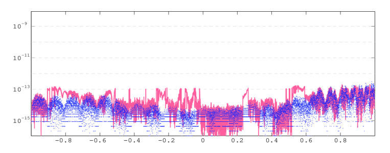
Figure 1: The graph of the absolute error (dark blue dots) of the approximation to the integral (2.1) for $f(x)=\sin(33x)+\exp(\sin(\mathsf{e}^{4x}))$, computed for $19999$ equidistant values of $\tau\in(-1,1)$ using only (2.5) and the adaptive quadrature quadgk from the Matlab system, and the graph of the numerical estimation of this error (irregular light red line) computed by the adaptive quadrature itself.

Figure 2 presents the results obtained for the same integral, but with the tolerance control and the error estimates (4.31)–(4.34) turned back on. Now, the error is safely estimated, the gap between the estimation line and the ”cloud” of actual errors varies from about $1$ decimal digit (for $\tau$’s near the endpoints) to about $2$ decimal digits (for $\tau$’s near the centre of the interval). One may fault that the estimation is not tight enough, if $\tau$ lies in the middle part of the interval. This is because the computation of values of the function $f_{8}$ is, despite its complicated formula, quite stable. Moreover, in this example, the round-off errors that appear during the computation of values of the functions $g$ and $h$ in (2.6) depend more on $|\varepsilon x|$ than on $\varepsilon$, while the latter is assumed in our error estimations. To illustrate it more clearly, in the next experiment, we compute the integrals (2.1) for $f\equiv f_{9}$, where

$$f_{9}(x)=f_{8}(j(x)),\quad\mathrm{and}\quad j(x)=\arcsin(\sin(2\pi+x)).$$ (5.5)

Clearly, in theory, $j(x)=x$ for every $x\in[-\pi,\pi]$, and, consequently, $I_{\tau}(f_{9})=I_{\tau}(f_{8})$ for each $\tau\in(-1,1)$. However, the computation of values of the function $f_{9}$ is much less stable than in the case of $f_{8}$. The graph of the absolute error (and its estimation) of the approximation to the integral (2.1) with $f\equiv f_{9}$, computed using the proposed method, can be found in Figure 3. The error estimation reflects the behaviour of the actual error very well. The error nowhere exceeds its estimation, and the distance between them is greater than $0.1$ of decimal digit for all values of $\tau$.

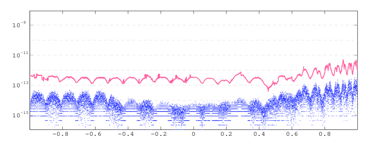
Figure 2: The graph of the absolute error (dark blue dots) of the approximation to the integral (2.1) for $f(x)=\sin(33x)+\exp(\sin(\mathsf{e}^{4x}))$, computed for $19999$ equidistant values of $\tau\in(-1,1)$ using (4.22) and the adaptive quadrature quadgk from the Matlab system, and the graph of the numerical estimation of this error (irregular light red line) computed according to (4.23)–(4.24), (4.31) with (5.2), and (4.32)–(4.34).

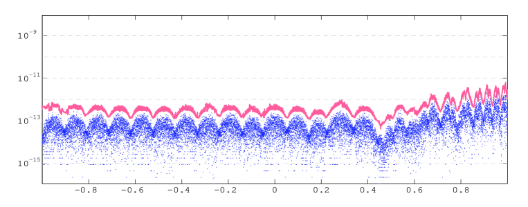
Figure 3: The graph of the absolute error (dark blue dots) of the approximation to the integral (2.1) for $f(x)=f_{8}(j(x))$, where $f_{8}(x)=\sin(33x)+\exp(\sin(\mathsf{e}^{4x}))$ and $j(x)=\arcsin(\sin(2\pi+x))$, computed for $19999$ equidistant values of $\tau\in(-1,1)$ using (4.22) and the adaptive quadrature quadgk from the Matlab system, and the graph of the numerical estimation of this error (irregular light red line) computed according to (4.23)–(4.24), (4.31) with (5.2), and (4.32)–(4.34).

In the final test involving the quadgk adaptive quadrature, we consider once again the function $f_{5}$ (5.4) which is difficult for two reasons. It is a nearly singular function, and, what is numerically very dangerous in this example, the constant $1.00001$ does not have an accurate representation in the double precision arithmetic. The graphs of the absolute error of the approximation to the integral $I_{\tau}(f_{5})$ and its estimation computed using the proposed method are presented in Figure 4.

In the case the computation of the values of the function $f$ in (2.1) is very unstable, the proposed method may fail to compute a reliable error estimation (as, practically, almost every other method). However, by the presented examples, we may conclude that the proposed error estimates seem to be a very reasonable practical choice.

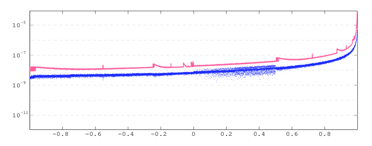
Figure 4: The graph of the absolute error (dark blue dots) of the approximation to the integral (2.1) for $f(x)=\frac{1}{100}(x-1.00001)^{-2}$, computed for $19999$ equidistant values of $\tau\in(-1,1)$ using (4.22) and the adaptive quadrature quadgk from the Matlab system, and the graph of the numerical estimation of this error (irregular light red line) computed according to (4.23)–(4.24), (4.31) with (5.2), and (4.32)–(4.34).

Another adaptive quadrature we have tested our method with, is the quadcc algorithm based on the results given in [6]. The quadcc function is not included in Matlab, but can be downloaded from the Matlab File Exchange webpage. The most significant difference between the quadgk and the quadcc adaptive quadratures is that the latter uses a nonlinear error estimator. In the quadcc algorithm, the integral (1.2) (over a single subinterval) is approximated using the $2^{k}+1$ point Clenshaw-Curtis quadratures for $k=2,3,4,5$. As the estimation of the quadrature error, the L²-norm of the difference between the integrand and the corresponding interpolant is used (the norm is approximated by means of Legendre polynomial expansion). Thus, considering the influence of round-off errors, a possible perturbation of the integrand at a quadrature node will more likely increase the value of the quadcc error estimate rather than partially cancel out with perturbations at other nodes (which is quite often in case of linear error estimators). This makes the adaptive quadrature very reliable, but may cause a considerable efficiency drop if the error tolerance is set too small.

The quadcc adaptive quadrature includes relative error control, which is a little inconvenient for us for the reasons described when presenting experiments in Maple. To solve the problem we may (as in the Maple implementation of our method) compute rough approximations to the two integrals in (2.5), and then use these values to ”convert” the absolute error tolerance into the relative one before calling the quadcc subroutine. On the other hand, in the quadcc algorithm, the verification whether the relative tolerance is met is done by checking the condition $E\leq T\hskip 0.86108pt|J|$, where $E$ is the current approximation of the absolute error, $T$ is the error tolerance, and $J$ is the most recent approximation of the integral. Just by modifying this condition to $E\leq T$, we may very easily change the relative error control to the absolute one. With both above solutions, we obtain the same numerical results. However, with the latter (which we use in our experiments) we save some computation time.

Formally, quadcc is the closed type adaptive quadrature, but it also features the properties of the open type one. This duality is achieved by removing the node at which an infinite (or undefined) value of the integrand is encountered from the set of nodes, and then recalculating the quadrature weights. Therefore, using the quadcc subroutine, we also can apply the algorithm based on (4.22) for approximating the integral (2.1). In the next two experiments, we are going to verify whether our suspicion that the average case error estimate (4.31) may not be applicable for controlling the error tolerance of an adaptive quadrature equipped with a nonlinear error estimator (cf. the discussion at the end of Section 4.2.1).

To this end, we have computed $19999$ values of the integral $I_{\tau}(f_{9})$ (cf. (5.5)) by the similar algorithm as when using the quadgk function. In the first experiment, the error tolerance for the quadcc subroutine was controlled by the pessimistic error estimate (4.29) (under the assumption that $x_{00}>\varepsilon^{1/2}$), in the second one – by the average case estimate (4.31). In both cases, the distribution of the actual approximation error is very similar, while – of course – the computed error estimation (which is often the only information for the user about the accuracy of the approximation) is considerably different. The results are presented in Figure 5.

As we could expect, the error tolerance based on the inequality (4.31) turned out to be a little too small for the quadcc algorithm. Switching from the pessimistic error tolerance to the average case one caused a huge efficiency drop. The computation time increased by almost $1400\%$ (for comparison, when performing similar experiments involving the quadgk subroutine which uses the linear error estimator, the analogous growth of the computation time was only $10\%$). However, we have observed that by only slightly releasing the error tolerance, i.e. multiplying the right hand side of (4.31) by $2$, the increase of the computation time may be considerably decreased (to only $250\%$ in the considered example, which seems to be an acceptable price for obtaining much more tight error estimation).

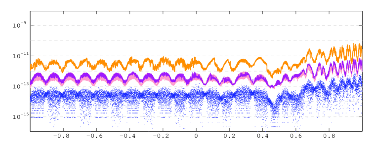
Figure 5: The graph of the absolute error (dark blue dots) of the approximation to the integral (2.1) with $f(x)=f_{8}(j(x))$, where $f_{8}(x)=\sin(33x)+\exp(\sin(\mathsf{e}^{4x}))$ and $j(x)=\arcsin(\sin(2\pi+x))$, computed for $19999$ equidistant values of $\tau\in(-1,1)$ using (4.22) and the adaptive quadrature quadcc [6], and the graph of the error estimation computed using (4.23)–(4.24), (4.31) with (5.2), and (4.32)–(4.34) in the case the error tolerance was controlled by: a) (4.29) (irregular light orange line), b) (4.31) (irregular pale red line), c) (4.31)$\times 2$ (irregular purple line). The graph of the actual error corresponds to the case c), however is very similar in both other cases.

The proposed method based on the quadcc adaptive quadrature is considerably slower than the analogous one that uses the quadgk subroutine (from a few to several dozen times, depending on the regularity of the integrand). However, the error estimator of the quadcc subroutine, responsible for estimating the errors $E_{A}(\cdot,\cdot,\cdot)$ in (4.19) or (4.23), is extremely reliable. The proposed algorithm in connection with the quadgk quadrature offers a very reasonable level of reliability, but examples can be found, where the error estimator in the quadgk algorithm fails, causing our method to return incorrect (too small) error estimation. When testing the proposed method with the quadcc adaptive quadrature, we did not find an integral of the form (2.1) for which the approximation error would have been falsely estimated.

While presenting the results of Matlab experiments, we have concentrated on the method presented in Section 4.2. With any reliable, open or closed type, adaptive quadrature we may successfully apply the algorithm based on (4.18)–(4.19). The results of such an experiment for the adaptive quadrature quadcc in the case of the integral $I_{\tau}(f_{9})$ are presented in Figure 6 (when applying the quadgk subroutine, the results are almost identical). The distance between the approximation error and its estimation is larger than $0.35$ of decimal digit for all values of $\tau$. As we can also see, the graphs of the error estimation and the actual error are very regular. This is because the most significant part of the approximation error is related to the removal of the interval $[\tau-\mu,\tau+\mu]$ from the interval of integration (the last term in (4.19)). For the same reason, the approximation error is larger than the one we obtain when applying the approach presented in Section 4.2.

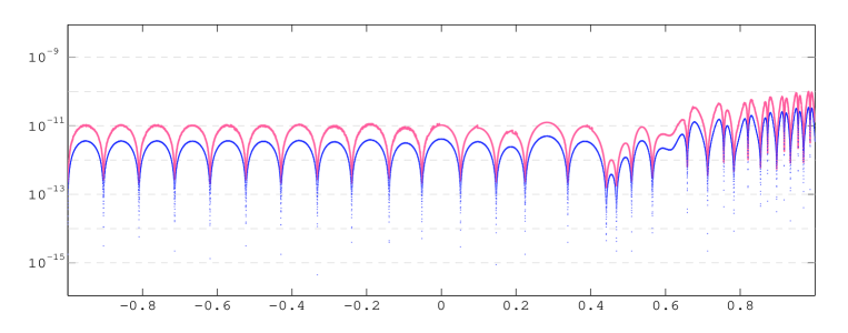
Figure 6: The graph of the absolute error (dark blue dots) of the approximation to the integral (2.1) with $f(x)=f_{8}(j(x))$, where $f_{8}(x)=\sin(33x)+\exp(\sin(\mathsf{e}^{4x}))$ and $j(x)=\arcsin(\sin(2\pi+x))$, computed for $19999$ equidistant values of $\tau\in(-1,1)$ using (4.18) and the adaptive quadrature quadcc, and the graph of the error estimation (red solid line) computed according to (4.19) (with $\mu$ satisfying (4.21)), (5.2), and (4.32)–(4.34).

5.3 The present method versus qawc

In this paper, we have applied a standard (designed for evaluating the integrals of the form (1.2)) adaptive quadrature to compute the Cauchy principal value integrals. An adaptive quadrature designed specially for computing the integrals (1.1) was included in Quadpack [18]. The subroutine is called qawc and is still used quite frequently.

The qawc algorithm uses two types of quadratures. The $25$-point generalized Clenshaw-Curtis quadrature for evaluating the integral in the subinterval containing the singularity point, and the well known $15$-point Kronrod extension of the $7$-point Gauss-Legendre quadrature. The algorithm includes empirical round-off error detection. If the estimated approximation error is too large compared to the value of the integral in too many subintervals, the qawc subroutine reports a failure. For the experiment, we have used the Matlab translation of qawc from the Slatec library.

We have tested the qawc adaptive subroutine for three different functions $f$ in (2.1): $f\equiv f_{5}$ (5.4), $f\equiv f_{9}$ (5.5), and $f\equiv f_{10}(x)=100\hskip 0.86108pt(x+1/2)^{2}$. The error tolerance was set to $\sqrt{\varepsilon}$ in the case of the function $f_{5}$, and to $1000\varepsilon$, otherwise. The assumed error tolerances are a little too small to be reached, so we can verify how well the round-off errors are detected by the qawc algorithm. The results are not satisfactory (see Figure 7). For the integrals $I_{\tau}(f_{5})$ and $I_{\tau}(f_{10})$, the approximation error was falsely estimated for $15171$ and $9056$ of $19999$ values of $\tau$, respectively. The best results were obtained in the case the integral $I_{\tau}(f_{9})$, the approximation error was estimated incorrectly for only $144$ values of $\tau$, and in $1694$ cases the qawc function reported a failure. For higher error tolerances, the results improved, but only in the case of functions $f_{5}$ and $f_{9}$. We have found that, in general, the qawc algorithm computes quite reliable results, if a correct error tolerance $T_{{\tt qawc}}$ is set, and the absolute error is estimated by $\max\{T_{{\tt qawc}},E_{{\tt qawc}}\}$ instead of $E_{{\tt qawc}}$, where $E_{{\tt qawc}}$ corresponds to the error estimate reported by the qawc function. In the last graph of Figure 7, we present the results of the experiment involving the integral $I_{\tau}(f_{9})$ again. This time however, the proper error tolerance $T_{{\tt qawc}}$ was set according to (4.31) and (4.33)–(4.34), while the approximation error was estimated as described above. The integral was computed correctly for all values of $\tau$. With this scheme, the correct results were also obtained in the case of the other tested integrals. As far as the efficiency is concerned, the qawc subroutine turned out to be slower than the proposed method using the quadgk or the quadcc adaptive quadrature.

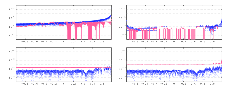
Figure 7: The graphs of the absolute error (dark blue dots) of the approximation to the integral (2.1), and the graphs of the error estimation (irregular light red line) computed by the qawc algorithm from Quadpack [18] in the case a) $f(x)=f_{5}(x)$ (5.4) and the error tolerance $T_{{\tt qawc}}=\sqrt{\varepsilon}$ (upper-left graph), b) $f(x)=100\hskip 0.77498pt(x+1/2)^{2}$ and the error tolerance $T_{{\tt qawc}}=1000{\varepsilon}$ (upper-right graph), c) $f(x)=f_{9}(x)$ (5.5) and the error tolerance $T_{{\tt qawc}}=1000{\varepsilon}$ (lower-left graph). The last graph also presents the results for $f\equiv f_{9}$, but in the case the error tolerance and the error estimation of the qawc subroutine were supported by the estimates proposed in this paper.

6 Conclusions and final thoughts

We have shown that a fine ordinary adaptive quadrature can be successfully used for fast and accurate computations of the Cauchy principal value integrals, if the error tolerance for the adaptive quadrature and the reported error estimation remain under control of the error estimates proposed in this paper.

The presented method works most efficiently when used with an adaptive quadrature using a linear error estimator. Such adaptive quadratures, however, may sometimes accidentally fail to compute a reliable approximation. The probability of such a failure may be considerably decreased by setting very small error tolerance. On the other hand, if the tolerance is too small, the result may be quite the opposite, as also the efficiency of the adaptive quadrature may drop significantly. In the present paper, we give tools that enable the automatic selection of ”near optimal” error tolerance, ensuring high level of reliability and high efficiency of the proposed algorithm.

A small disadvantage of the presented method is that some knowledge on the given adaptive quadrature is required for a proper selection of constants the proposed error estimates are based on. In addition, not every adaptive quadrature can be used together with the proposed method. Such a quadrature should exhibit a stable behaviour in the presence of round-off errors. We do not require the adaptive quadrature to correctly estimate the influence of these errors (the error estimates derived in this paper are meant to do so). The quadrature, however, should not miss the accurate result by considerably more than the influence of the round-off errors justifies.

References

- [1] P. Billingsley, Probability and Measure, 3rd ed., Wiley, New York, 1995.
- [2] R. M. Corless, G. H. Gonnet, D. E. G. Hare, D. J. Jeffrey, and D. E. Knuth, On the Lambert W Function, Adv. Comput. Math. 5 (1996), 329–359.
- [3] P. J. Davis and P. Rabinowitz, Methods of Numerical Integration, 2nd ed., Academic Press, New York, 1984.
- [4] D. Elliott and D. F. Paget, Gauss type quadrature rules for Cauchy principal value integrals, Math. Comp. 33 (1979), 301–309.
- [5] P. Gonnet, Adaptive quadrature re-revisited, Ph.D. thesis, ETH Zürich, Switzerland, 2009.
- [6] P. Gonnet, Increasing the reliability of adaptive quadrature using explicit interpolants, ACM Transactions on Mathematical Software (TOMS), 37(3) (2010), Article No. 26.
- [7] P. Gonnet, A review of error estimation in adaptive quadrature, ACM Computing Surveys (CSUR), 44(4) (2012), Article No. 22.
- [8] T. Hasegawa and T. Torii, An automatic quadrature for Cauchy principal value integrals, Math. Comp. 56 (1991), 741–754.
- [9] G. He, S. Xiang, An improved algorithm for the evaluation of Cauchy principal value integrals of oscillatory functions and its application, J. Comput. Appl. Math. 280 (2015) 1–13.
- [10] P. Keller, Round-off errors in the problem of computing Cauchy principal value integrals (2011), arXiv:1111.2283.
- [11] P. Keller, A practical algorithm for computing Cauchy principal value integrals of oscillatory functions, Appl. Math. Comput. 218 (2012), 4988-5001.
- [12] A. S. Kronrod, Nodes and Weights of Quadrature Formulas, Consultants Bureau, New York, 1965.
- [13] I. M. Longman, On the numerical evaluation of Cauchy principal values of integrals, MTAC 12 (1958), 205–207.
- [14] S. K. Mitra, On the probability distribution of the sum of uniformly distributed random variables, SIAM J. Appl. Math., 20(2) (1971), 195–198.
- [15] G. Monegato, The numerical evaluation of one-dimensional Cauchy principal value integrals, Computing 29 (1982), 337–354.
- [16] D. F. Paget and D. Elliott, An algorithm for the numerical evaluation of certain Cauchy principal value integrals, Numer. Math. I9 (1972), 373–385.
- [17] R. Piessens, Numerical evaluation of Cauchy principal values of integrals, BIT 10 (1970), 476–480.
- [18] R. Piessens, E. deDoncker-Kapenga, C. W. Überhuber, and D. K. Kahaner, QUADPACK, A subroutine package for automatic integration, Springer-Verlag, Berlin, 1983.
- [19] L. F. Shampine, Vectorized adaptive quadrature in MATLAB, J. Comput. Appl. Math. 211 (2008), 131–140.
- [20] L. F. Shampine, R. C. Allen Jr., S. Pruess, Fundamentals of Numerical Computing, Wiley, NewYork, 1997.
- [21] C. E. Stewart, On the numerical evaluation of singular integrals of Cauchy type, J. Soc. Indust. Appl. Math. 8(2) (1960) 342–353.
- [22] H. Wang, S. Xiang, On the evaluation of Cauchy principal value integrals of oscillatory functions, J. Comput. Appl. Math. 234 (2010) 95–100.