Implications of Recent Data on Neutrino Mixing and
Lepton Flavour Violating Decays for the Zee Model

Abstract

We study implications of recent data on neutrino mixing from T2K, MINOS, Double Chooz and $\mu\to e\gamma$ from MEG for the Zee model. The simplest version of this model has been shown to be ruled out by experimental data some time ago. The general Zee model is still consistent with recent data. We demonstrate this with a constrained Zee model based on naturalness consideration. In this constrained model, only inverted mass hierarchy for neutrino masses is allowed, and $\theta_{13}$ must be non-zero in order to have correct ratio for neutrino mass-squared differences and for mixing in solar and atmospherical neutrino oscillations. The best-fit value of our model for $\theta_{13}$ is $8.91^{\circ}$ from T2K and MINOS data, very close to the central value obtained by Double Chooz experiment. There are solutions with non-zero CP violation with the Jarlskog parameter predicted in the range $\pm 0.039$, $\pm 0.044$ and $\pm 0.048$ respectively for a 1$\sigma$, 2$\sigma$ and 3$\sigma$ ranges of other input parameters. However, without any constraint on the $\theta_{13}$-parameter above respective ranges become $\pm 0.049$, $\pm 0.053$ and $\pm 0.056$. We analyse different cases to obtain a branching ratio for $\mu\to e\gamma$ close to the recent MEG bound. We also discuss other radiative as well as the charged trilepton flavour violating decay modes of the $\tau$-lepton.

I Introduction

The standard model (SM) of electroweak and strong interactions based on the gauge group $SU(3)_{C}\times SU(2)_{L}\times U(1)_{Y}$ has been rigorously tested in many ways, in different sectors involving gauge bosons, quarks and leptons. The flavour physics in the quark sector including CP violation is well described by the Cabbibo-Kobayashi-Maskawa (CKM) mixing matrix in the charged current interactions of the W boson with three generations of quarks. Corresponding interactions in the leptonic sector are not on the same footing. In the simplest version of the SM, there are no right handed neutrinos and the left handed neutrinos are massless. This theory conserves lepton number of each family separately, and no flavour changing neutral current (FCNC) processes are allowed in the leptonic sector. However, the observation of neutrino oscillations requires both neutrino masses and flavour changing processes.

Study of neutrino oscillations in the past few years has led to an insight regarding mass differences and mixing between the three light neutrinos. The SM can be easily extended to give neutrino masses and explain their mixing through a mixing matrix in the charged lepton currents analogous to the CKM matrix in the quark sector as was first suggested by Pontecorvo-Maki-Nakagawa-Sakata (PMNS) pmns . Experimentally, not all the parameters of this matrix are known; in particular whether CP is violated in the leptonic sector. Further understanding of the smallness of neutrino masses requires new physics, such as loop induced masses as in the Zee model Zee , or a seesaw mechanism which can be implemented in several ways, referred to as Type I Ref:SeesawI , II Ref:SeesawII , III Ref:SeesawIII seesaw models. These models, besides generating neutrino masses and their mixing, also induce other FCNC processes in the leptonic sector causing new lepton flavour violation (LFV) phenomena. There are strong constraints on LFV interaction PDG . The Zee model has been extensively studied in the literature Petcov:1982en . Data from T2K T2K and MINOS MINOS a few months ago provided some new information on the mixing angles in $V_{PMNS}$ that the last mixing angle $\theta_{13}$ is non-zero at more than 2$\sigma$ level. The combined data analysis gives the confidence level at more than 3$\sigma$ which put the well known tri-bimaximal mixing pattern into question. Very recent data from Double Chooz chooze also indicate that $\theta_{13}$ may be non-zero. Models for neutrino masses and mixing are therefore further constrained. The hint of non-zero $\theta_{13}$ sparks a few analysis in various ways, see for example Bhattacharyya:2011zv . In most of the models for neutrino masses and mixing, there are LFV interactions. For a study of testing a model, it is therefore also necessary to consider LFV processes. Recently MEG collaboration MEG has report a new upper bound of $2.4\times 10^{-12}$ for $\mu\to e\gamma$ branching ratio which is about 5 times better than previous one PDG . This improved upper bound may have implications on models for neutrino mass and mixing. In this work we confront the Zee model with the new data on neutrino mixing and different LFV processes.

I.1 The Zee model

Neutrinos being electrically neutral allows the possibility that they are Majorana particles. There are many ways to realize Majorana neutrino masses. Even with the restrictive condition of renormalizability, there are different type of models. Without introducing right-handed neutrino $N_{R}$, one can generate Majorana neutrino masses by introducing Higgs representations. With different Higgs representations, one can generate neutrino masses at the tree or loop levels. The Zee model is a very economic model for loop induced neutrino masses providing some reasons why neutrino masses are so much smaller than their charged lepton partners.

In the Zee model, in addition to the minimal SM without right-handed neutrinos, there is another Higgs scalar doublet representation $\Phi_{2}:(1,2,1)$ beside the doublet $\Phi=\Phi_{1}$ already in the minimal SM, and a charged scalar singlet $h^{+}:(1,1,2)$. Terms in the Lagrangian relevant to lepton masses are

$$L=-\bar{L}_{L}(f^{\dagger}_{1}\Phi_{1}+f^{\dagger}_{2}\Phi_{2})E_{R}-\bar{L}^{c}_{L}fi\sigma_{2}L_{L}h^{+}-\mu\Phi_{1}^{\dagger}\,i\,\sigma_{2}\Phi^{*}_{2}h^{+}+h.c.$$ (1)

where $L^{c}_{L}=C\bar{L}_{L}^{T}$ is the charge conjugated $L_{L}:(1,2,-1)$, $E_{R}:(1,1,-2)$ is the $SU(2)-$singlet right-handed charged lepton and $\mu$ is the tri-scalar coupling constant with mass-dimension one. The Yukawa coupling matrices $f_{i}$ are arbitrary while $f$ is anti-symmetric in exchanging the family indices.

This leads to a mass matrix for the charged leptons

$$m_{E}=\frac{v}{\sqrt{2}}(\rm sin\beta f^{\dagger}_{1}+\rm cos\beta f^{\dagger}_{2})\;,$$ (2)

where $v=\sqrt{v^{2}_{1}+v^{2}_{2}}$ and $\rm tan\beta=v_{1}/v_{2}$ with

$$\Phi_{i}=\begin{pmatrix}\phi_{i}^{+}\\ \frac{1}{\sqrt{2}}(v_{i}+\phi^{0}_{Ri}+i\phi^{0}_{Ii})\end{pmatrix}.$$ (3)

We will work in the basis where charged-lepton mass matrix, $m_{E}$, is diagonalised, such that $m_{E}={\rm diag}(m_{e},m_{\mu},m_{\tau})$.

The would-be Goldstone bosons $w^{+}$ and $z$ “eaten” by the $W^{+}$ and $Z$ bosons and the other two physical components, $H^{+}$ and $a$ are given by

$$\begin{pmatrix}H^{+}\\ w^{+}\end{pmatrix}=\begin{pmatrix}\rm cos\beta&-\rm sin\beta\\ \rm sin\beta&\rm cos\beta\end{pmatrix}\begin{pmatrix}\phi_{1}^{+}\\ \phi_{2}^{+}\end{pmatrix},\quad\begin{pmatrix}a\\ z\end{pmatrix}=\begin{pmatrix}\rm cos\beta&-\rm sin\beta\\ \rm sin\beta&\rm cos\beta\end{pmatrix}\begin{pmatrix}\phi^{0}_{I1}\\ \phi^{0}_{I2}\end{pmatrix}.$$ (4)

For the two CP even fields $\phi_{R1,R2}$, we will use their mass eigen-states $H$ and $h$ linear combinations,

$$\begin{pmatrix}H\\ h\end{pmatrix}=\begin{pmatrix}\rm cos\alpha&-\rm sin\alpha\\ \rm sin\alpha&\rm cos\alpha\end{pmatrix}\begin{pmatrix}\phi^{0}_{R1}\\ \phi^{0}_{R2}\end{pmatrix}.$$ (5)

There will be mixing between $H^{+}$ and $h^{+}$ if $\mu$ is not zero. Without loss of generality, one can write the mass eigen-states $h^{+}_{1}$ and $h^{+}_{2}$ as

$$\begin{pmatrix}h^{+}_{1}\\ h^{+}_{2}\end{pmatrix}=\begin{pmatrix}\rm cos\theta_{z}&-\rm sin\theta_{z}\\ \rm sin\theta_{z}&\rm cos\theta_{z}\end{pmatrix}\begin{pmatrix}h^{+}\\ H^{+}\end{pmatrix}.$$ (6)

We have the following lepton-scalar couplings,

$$L = -\bar{\nu}_{L}\left({\sqrt{2}m_{E}\over v\rm tan\beta}-{f^{\dagger}_{2}\over\rm sin\beta}\right)E_{R}(-\rm sin\theta_{z}h^{+}_{1}+\rm cos\theta_{z}h^{+}_{2})$$ (7)

$$-2\bar{\nu}_{L}^{c}fE_{L}(\rm cos\theta_{z}h^{+}_{1}+\rm sin\theta_{z}h^{+}_{2})$$

$$-\bar{E}_{L}\left({m_{E}\rm sin\alpha\over v\rm sin\beta}+\rm sin(\beta-\alpha){f^{\dagger}_{2}\over\sqrt{2}\rm sin\beta}\right)E_{R}h$$

$$-\bar{E}_{L}\left({m_{E}\rm cos\alpha\over v\rm sin\beta}-\rm cos(\beta-\alpha){f^{\dagger}_{2}\over\sqrt{2}\rm sin\beta}\right)E_{R}H$$

$$-i\,\bar{E}_{L}\left({m_{E}\over v\rm tan\beta}-{f^{\dagger}_{2}\over\sqrt{2}\rm sin\beta}\right)E_{R}a+h.c.\;.$$

The neutrino mass matrix, defined by $(1/2)\bar{\nu}_{L}^{c}\hat{M}_{\nu}\nu_{L}$, is related to the model parameters as

$$M_{\nu}=U^{*}\hat{M}_{\nu}U^{\dagger}=\mbox{A}\left(fm^{2}_{E}+m^{2}_{E}f^{T}-{v\over\sqrt{2}\rm cos\beta}(fm_{E}f_{2}+f_{2}^{T}m_{E}f^{T})\right)\;,$$ (8)

where $U=V_{PMNS}$ is the PMNS mixing matrix, and

$$\mbox{A}=\rm sin(2\theta_{z})\ln\left(m^{2}_{h_{2}^{+}}/m^{2}_{h^{+}_{1}}\right)/8\sqrt{2}\pi^{2}v\rm tan\beta.$$ (9)

In the simplest Zee model, $f_{2}=0$. It can be easily seen from the expression for $M_{\nu}$ that in this case, the resulting mass matrix has all diagonal entries to be zero. This type of mass matrix has been shown to be ruled out by data ruleout0f2 . This is basically because that it cannot simultaneously have solution for $|V_{\mu 3}|$ close to $1/\sqrt{2}$ and $|V_{e2}|$ close to $1/\sqrt{3}$ as data require. With $f_{2}$ non-zero it can fit experimental data. In this case, however, we encounter a problem which is common to many models beyond the SM: that there are too many new parameters. Additional theoretical considerations help to narrow down the parameter space. To this end, it has been proposed that an interesting mass matrix can result if one imposes the requirement that no large hierarchies among the new couplings, that is, all $f^{ij}$ and $f^{ij}_{2}$ are of the same order of magnitude, respectively, from naturalness consideration. From the expression for the neutrino mass matrix one sees that all terms are either proportional to charge lepton mass $m_{l}$ or mass-squared $m^{2}_{l}$. Since $m_{\tau}>>m_{\mu},m_{e}$, the leading contributions to the neutrino mass matrix are proportional to $f^{i\tau}m^{2}_{\tau}$ and $f^{\tau i}_{2}m_{\tau}$. To this order, one can write the neutrino mass matrix using the five input parameters $x,y,z,a$ and $\delta$ only, without loss of generality, as

$$M_{\nu}=a\left(\begin{array}[]{ccc}1&(ye^{i\delta}+x)/2&z\\ (ye^{i\delta}+x)/2&xye^{i\delta}&xz\\ z&xz&0\\ \end{array}\right)\;.$$ (13)

Here $a$ is the absolute value of the 11 entry $M_{11}$,

$$M_{11} = -2Avm_{\tau}f^{e\tau}f^{\tau e}_{2}/\rm cos\beta,$$ (14)

of $M_{\nu}$ and $z$ is the absolute value of 13 entry $M_{13}$ divided by $a$ with

$$M_{13} = Af^{e\tau}m_{\tau}(m_{\tau}-vf^{\tau\tau}_{2}/\rm cos\beta),$$ (15)

$x=|f^{\mu\tau}|/|f^{e\tau}|$ is the absolute value of the ratio of $M_{23}$ to $M_{13}$ and $y=|M_{22}|/xa$ with

$$M_{22} = -2Avm_{\tau}f^{\mu\tau}f^{\tau\mu}_{2}/\rm cos\beta.$$ (16)

One can choose a convention where all the above parameters are real except $f^{\tau\mu}_{2}$.

II Neutrino masses and mixing

The mass matrix $M_{\nu}$ is of rank two with the two eigen masses given by

$$m^{2}_{\pm} = {a^{2}\over 4}\left(|1+xye^{i\delta}|^{2}+(1+x^{2})(1+y^{2}+4z^{2})\right.$$ (17)

$$\left.\pm 2|1+xye^{i\delta}|\sqrt{(1+x^{2})(1+y^{2}+4z^{2})}\right)\;.$$

If one identifies $m_{1}=m_{-}$, $m_{2}=m_{+}$ and $m_{3}=0$, the corresponding $V_{PMNS}$ mixing matrix is given by

$$V_{PMNS}=\left(\begin{array}[]{lll}{B-(1+xye^{i\delta})\over\sqrt{2}N_{1}}&-{B+(1+xye^{i\delta})\over\sqrt{2}N_{2}}&{2xz\over N_{3}}\\ {xB-(1+xye^{i\delta})ye^{-i\delta}\over\sqrt{2}N_{1}}&-{xB+(1+xye^{i\delta})ye^{-i\delta}\over\sqrt{2}N_{2}}&-{2z\over N_{3}}\\ -{\sqrt{2}(1+xye^{i\delta})z\over N_{1}}&-{\sqrt{2}(1+xye^{i\delta})z\over N_{2}}&{ye^{i\delta}-x\over N_{3}}\end{array}\right)\;,$$ (21)

where

$$B= |1+xye^{i\delta}|\sqrt{(1+y^{2}+4z^{2})/(1+x^{2})}\;,$$

$$N_{1,2}= |1+xye^{i\delta}|\left((1+y^{2}+4z^{2})\mp|1+xye^{i\delta}|\sqrt{(1+y^{2}+4z^{2})/(1+x^{2})}\right)^{1/2}\;,$$

$$N_{3}= \left((1+x^{2})(1+y^{2}+4z^{2})-|1+xye^{i\delta}|^{2}\right)^{1/2}\;.$$ (22)

Other identification would imply exchanges of column vectors in the above mixing matrix.

The non-zero masses in the above basis have Majorana phases. They are

$$\tilde{m}_{\pm}={a\over 2}(1+xye^{i\delta})\left(1\pm\sqrt{(1+x^{2})(1+y^{2}+4z^{2})/|1+xye^{i\delta}|^{2}}\right)\;.$$ (23)

Since $m_{3}=0$, the Majorana phase matrix $P$ can be written as $P\equiv{\rm diag}(1,e^{i\alpha},1)$. The simple structure of our model allows us to determine the Majorana phase $\alpha$ analytically. We defined the Majorana phase with the standard Particle Data Group (PDG) form for mixing matrix $V_{\rm PMNS}$PDG , where the e1- and e2-elements are real. With the help of the equation, $M_{\nu}=(V_{\rm PMNS}P)^{*}m^{\rm diag}(V_{\rm PMNS}P)^{\dagger}$, one can have the following relation

$${V^{*}_{e1}}^{2}m_{1}+{V^{*}_{e2}}^{2}m_{2}e^{-2\alpha}=M_{11}.$$ (24)

With the fact that the mass ratio $m_{2}/m_{1}$ is real and negative, we obtain

$${\rm cot}\alpha = \frac{2xy\rm sin\delta(1+x^{2})(1+xy\rm cos\delta)}{(y^{2}-x^{2}+4z^{2})(1+x^{2}+y^{2}+2xy\rm cos\delta)}\;.$$ (25)

The Jarlskog parameter $J=Im(V_{e1}V^{*}_{e2}V_{\mu 1}^{*}V_{\mu 2})$ is given by

$$J = -{2xyz^{2}\sqrt{1+x^{2}}\rm sin\delta\over((1+x^{2})(1+y^{2}+4z^{2})-|1+xye^{i\delta}|^{2})|1+xye^{i\delta}|\sqrt{(1+y^{2}+4z^{2})}}$$ (26)

$$= -{a^{4}xyz^{2}(1+x^{2})\rm sin\delta\over 2(m^{2}_{+}-m^{2}_{-})\sqrt{m^{2}_{+}m^{2}_{-}}}\;.$$

This model only allows inverted neutrino mass hierarchy solution with $m_{1}$ and $m_{2}$ identified with $m_{-}$ and $m_{+}$ in the above, and $m_{3}=0$. For normal neutrino mass hierarchy, that is $m_{1}=0$, one would require the 13 entry, $xz/N_{3}=|V_{e1}|$, to be of order $\sqrt{2/3}$ and the 12 entry, $|(B+(1+xye^{i\delta})/\sqrt{2}N_{2}|=|V_{e3}|$, to be small in eq.(21). Combining with the information that $\Delta m^{2}_{21}/\Delta m^{2}_{32}=m^{2}_{-}/(m^{2}_{+}-m^{2}_{-})$ is small, we find that there is no solution.

With known ranges for $|V_{e2}|$, $|V_{\mu 3}|$, and $\Delta m^{2}_{21}/\Delta m^{2}_{32}$, even without knowing the value for $V_{e3}$, it is constrained to be non-zero at more than 1$\sigma$ level. This model requires a non-zero $V_{e3}$ in consistent with T2K, MINOS and Double Chooz data.

Parameter	$\delta m^{2}/10^{-5}{\rm eV}^{2}$	$\Delta m^{2}/10^{-3}{\rm eV}^{2}$	${\rm sin}^{2}\theta_{12}$	${\rm sin}^{2}\theta_{23}$	${\rm sin}^{2}\theta_{13}$
Best-fit	7.58	2.35	0.312	0.42	0.025
1$\sigma$ range	7.32 - 7.80	2.26 - 2.47	0.296 - 0.329	0.39 - 0.50	0.018 - 0.032
2$\sigma$ range	7.16 - 7.99	2.17 - 2.57	0.280 - 0.347	0.36 - 0.60	0.012 - 0.041
3$\sigma$ range	6.99 - 8.18	2.06 - 2.67	0.265 - 0.364	0.34 - 0.64	0.005 - 0.050

Table 1: Ranges for mixing parameters obtained in Ref.Fogli . The two mass-square differences are defined as $\delta m^{2}=m_{2}^{2}-m_{1}^{2}$ and $\Delta m^{2}=m_{3}^{2}-(m_{1}^{2}+m_{2}^{2})/2$

.

Evidence of non-zero reactor angle is published by T2K. When these data are combined with the data from MINOS and other experiments it clearly indicates a large deviation of the reactor angle form zero value Fogli Valle . In the following we present our results for allowed parameter space using the combined neutrino mixing data, including the recent T2K and MINOS results, given in Table-1 from Ref.Fogli with the new reactor flux estimate. The new Double Chooz data, $\rm sin^{2}(2\theta_{13})=0.085\pm 0.051$ is consistent with the ranges given in Table-1.

The best-fit values of the mass matrix parameters are:

$$x = 0.255,~{}~{}~{}y=4.100,~{}~{}~{}z=1.790,~{}~{}~{}a=0.017~{}{\rm eV},~{}~{}~{}\delta=180^{\circ},$$ (27)

and, the corresponding output for the mixing angles and mass-squared differences are given as follows

$$~{}~{}{\rm sin}^{2}\theta_{12}=0.3163,~{}~{}{\rm sin}^{2}\theta_{23}=0.4033,~{}~{}{\rm sin}^{2}\theta_{13}=0.0256,$$

$$~{}~{}\delta m^{2}=7.51\times 10^{-5}~{}{\rm eV^{2}}~{}~{}\Delta m^{2}=-2.36\times 10^{-3}~{}{\rm eV^{2}}.$$ (28)

The fact that our solutions are for inverted neutrino mass hierarchy case only is indicated by the negative sign on $\Delta m^{2}\left(=m_{3}^{2}-{\frac{(m_{2}^{2}+m_{1}^{2})}{2}}\right)$. In this case, solutions are in well agreement with $1\sigma$ range of experimental data of Table-1. However, there is no solution to be consistent with the normal hierarchy case. Using the T2K and MINOS data above the best-fit value of our model for $\theta_{13}$ is $8.91^{\circ}$, very close to the central value obtained by Double Chooz experiment.

Variation of input parameters $x,y,z,a$ and $\delta$ that satisfy the experimental neutrino data is shown in Fig.-1. In first row $x~{}{\rm vs}~{}y$, $x~{}{\rm vs}~{}z$ and $y~{}{\rm vs}~{}z$ are respectively shown in first, second and third plots. Input parameters are bounded to be within the larger-grey (purple-circle) area to generate neutrino data within 3$\sigma$ ranges. To satisfy neutrino data within 2$\sigma$ and 1$\sigma$ ranges, the input parameters have to be within the mid-white (yellow-triangle) and smaller-dark (red-star) areas respectively. We see here that the allowed range of the $x$-parameter lies in between $(0.23,~{}0.29)$, $(0.19,~{}0.34)$ and $(0.15,~{}0.40)$ for 1$\sigma$, 2$\sigma$ and 3$\sigma$ respectively. Corresponding limit on $y$-parameter one can read as $(4.0,~{}6.4)$, $(3.4,~{}13.6)$, $(3.2,~{}20.0)$ and that for the $z$-parameter is $(1.9,~{}2.8)$, $(1.6,~{}5.2)$, $(1.0,~{}8.0)$ respectively.

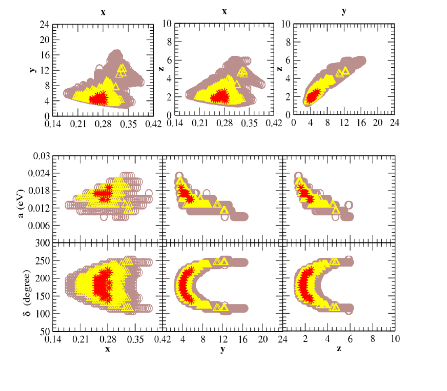
Figure 1: Variation of different input parameters (x, y, z, a, $\delta$ ) are shown here. Input parameters are bounded to be within the larger-grey (purple-circle) area to generate neutrino data within 3$\sigma$ range. To have neutrino data within 2$\sigma$ and 1$\sigma$ ranges, the input parameters will have to be within the mid-white (yellow-triangle) and smaller-dark (red-star) areas respectively.

On the second and third row, respectively, we have shown the variation of the parameters $a$ and $\delta$ with the $x$, $y$ and $z$-parameters. Here, we see that the parameter $a$ can be in between $(0.015~{}{\rm eV},~{}0.019~{}{\rm eV})$, $(0.011~{}{\rm eV},~{}0.020~{}{\rm eV})$ and $(0.007~{}{\rm eV},~{}0.023~{}{\rm eV})$ for 1$\sigma$, 2$\sigma$ and 3$\sigma$ respectively. The same for the CP-phase parameter $\delta$ is respectively given by $(140^{\circ},~{}210^{\circ}),~{}(110^{\circ},~{}230^{\circ})~{}{\rm and}~{}(100^{\circ}-250^{\circ})$ for 1$\sigma$, 2$\sigma$ and 3$\sigma$ with a central value at $180^{\circ}$.

The allowed range for $x~{}(=|f^{\mu\tau}|/|f^{e\tau}|)$ is a good evidence that our solutions are consistent with our naturalness assumption that the non-zero $f_{ij}$ should be the same order of magnitude.

The $(1,1)$ entry $m_{\nu_{ee}}$ of the neutrino mass matrix $M_{\nu}$ can induce neutrinoless double beta decay. In our model $m_{\nu_{ee}}=a$ is not zero, neutrinoless double beta decay can, therefore, happen. Experimentally, $m_{\nu_{ee}}$ is constrained to be $\raisebox{-1.72218pt}{\hbox to0.0pt{$\sim$\hss}}\raisebox{1.72218pt}{$<$}2~{}{\rm eV}$ PDG . In our analysis we see in Fig.-1 that the parameter $a$ is allowed upto $0.019~{}{\rm eV}$, $0.020~{}{\rm eV}$ and $0.023~{}{\rm eV}$ for 1$\sigma$, 2$\sigma$ and 3$\sigma$ cases respectively. Thus, our model is well below the allowed range for neutrinoless double beta decay effective neutrino mass parameter.

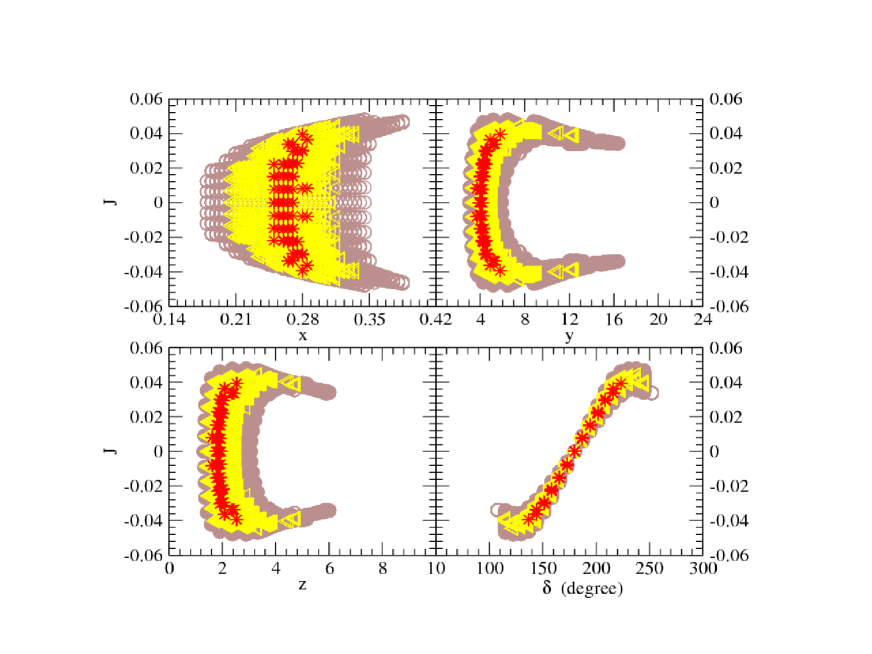
Figure 2: Variation of the Jarlskog parameter with different input parameters (x, y, z, $\delta$ ) are shown here. In this case neutrino mass-square differences as well as all three mixing angles, including $\theta_{13}$, are within the ranges set as given in Table-1.

There are some ongoing and planned experiments, for example GERDA Brugnera:2009zz and Majorana Phillips:2011db , to search for the neutrinoless double beta decay evidence. Both of these experiments are mainly intended to lower down the upper limit, $<2.2$ eV, on the effective mass parameter in the neutrinoless double beta experiment upto $0.1-0.3$ eV. These limits are much higher than the allowed range of the parameter “a”, $\sim 0.02$ eV, in our analysis. Thus, it will remain inconclusive in terms of the upper limit.

However, there is also a lower limit on the neutrinoless double beta decay effective mass parameter from the Heidelberg-Moscow experimentHeidel , $0.1~{}{\rm eV}\raisebox{-1.72218pt}{\hbox to0.0pt{$\sim$\hss}}\raisebox{1.72218pt}{$<$}~{}m_{ee}~{}\raisebox{-1.72218pt}{\hbox to0.0pt{$\sim$\hss}}\raisebox{1.72218pt}{$<$}~{}0.56~{}{\rm eV}$ at ($95\%$ C.L.). Once one include a $\pm~{}50\%$ uncertainty of the nuclear matrix elements, the above ranges widen to $0.05~{}{\rm eV}\raisebox{-1.72218pt}{\hbox to0.0pt{$\sim$\hss}}\raisebox{1.72218pt}{$<$}~{}m_{ee}~{}\raisebox{-1.72218pt}{\hbox to0.0pt{$\sim$\hss}}\raisebox{1.72218pt}{$<$}~{}0.84~{}{\rm eV}$ at ($95\%$ C.L.). The lower limit is much higher than the predicted range of “a” from our analysis. The main concern is that this result, the lower limit, is not confirmed by any other independent experiment. Here, GERDA in very near future during it’s phase-I will test the result claimed by the Heidelberg-Moscow experiment. This will be crucial for our discussion in terms of it’s lower limit. Our model parameters have to be reconsidered once the lower limit set by the Heidelberg-Moscow experiment is confirmed by GERDA during it’s phase-I run.

Consequence of a nonzero input phase $\delta$ will appear in the output Dirac CP-phase parameter. This is translated into a significant deviation of the Jarlskog parameter from zero value. We have shown the variation of the Jarlskog parameter in Fig.-2 with respect to the input parameters $x$, $y$, $z$ and $\delta$. We see that the allowed ranges of the Jarlskog parameter in our scenario lies in between $\pm 0.039$, $\pm 0.044$ and $\pm 0.048$ respectively for a 1$\sigma$, 2$\sigma$ and 3$\sigma$.

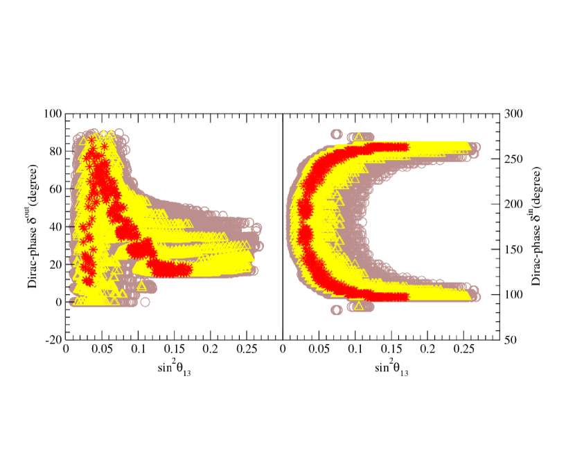
Figure 3: Variation of the output (left) and input (right) CP-phase with respect to the $\rm sin^{2}{\theta}_{13}$. Here, $\rm sin^{2}{\theta}_{13}$ is set to be free parameter while all other neutrino mixing angles as well as the mass-square differences are constrained.

One important outcome of our discussion is that the reactor angle is constrained to be nonzero. To have a clear picture, we have shown the variation of the $\rm sin^{2}\theta_{13}$ with respect to both the input and output phase angle in Fig.-3. In this figure $\rm sin^{2}{\theta}_{13}$ is free from any constraint while all other neutrino mixing angles as well as the mass-square differences are constrained to be within $1\sigma$, $2\sigma$ and $3\sigma$ ranges as given in Table-1. The variation of the output (input) CP-phase angle with $\rm sin^{2}{\theta}_{13}$ is shown on the left (right) panel in the figure. Here, we see that the lower limit on the reactor angle $\theta_{13}$ is clearly separated to be nonzero. The corresponding lower limit on the ${\rm sin}^{2}\theta_{13}$ are 0.024, 0.016 and 0.011 for 1$\sigma$, 2$\sigma$ and 3$\sigma$ cases. The best-fit value predicted from our analysis for $\theta_{13}$ comes out as $8.91^{\circ}$ which is very close to the central value obtained by Double Chooz experiment. In the same analysis, the Jarlskog parameter is constrained to be in between $\pm 0.049$, $\pm 0.053$ and $\pm 0.056$.

Finally, we consider the variation of the Majorana phase ($\alpha$), defined in eqn.(25), in terms of the input parameters $x$, $y$, $z$ and $\delta$. As before, here, we consider the variation in such a way that the input parameters lie within a range that will generate neutrino data in $1\sigma$, $2\sigma$ and $3\sigma$ as stated earlier. These three different respective zones are shown in Fig.-4, with same notation used in previous figures. The central value of the Majorana phase is around $-90^{\circ}$.

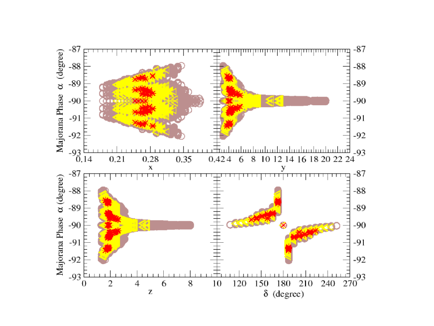
Figure 4: Variation of the Majorana phase with different input parameters (x, y, z, $\delta$ ) are shown here. The input parameters are within $1\sigma$, $2\sigma$ and $3\sigma$ ranges (see text).

III RADIATIVE FLAVOUR VIOLATING DECAYS ($\mu\to e\gamma$ and $\tau\to e(\mu)\gamma$)

In previous section, we have obtained allowed ranges for different input parameters that satisfy the current neutrino data. It is desirable to check whether these parameter space are compatible with other phenomenological aspects. From eqn.(7), we see that non-zero elements of two Yukawa coupling matrices $f_{2}$ and $f$ contribute to the LFV interactions mediated, respectively, via charged $(h^{+}_{1},h^{+}_{2})$ and neutral $(H,h,a)$ scalars as shown in Fig.-5. In this section we discuss a few such radiative decay modes, like, the $\mu\to e\gamma$ or $\tau\rightarrow\mu(e)\gamma$. Absence of any such lepton flavour violating process in SM, this analysis can impose stringent constraints on the parameters space.

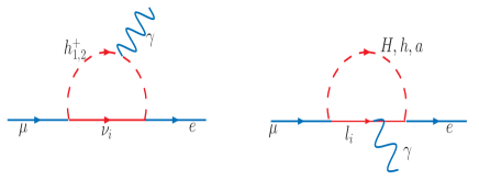
Figure 5: Diagrams contributing to the $\mu\rightarrow e\gamma$ process at the one loop level.

The matrix element $M$ for the decay mode $l_{i}\to l_{j}\gamma$ is given by,

$$M(l_{i}\to l_{j}\gamma)=ie\bar{f}_{j}(C^{ji}_{L}P_{L}+C^{ji}_{R}P_{R})\sigma_{\mu\nu}f_{i}\epsilon^{*}_{\mu}q_{\nu}\;,$$ (29)

here, $\epsilon$, being the photon polarisation vector and $\sigma_{\mu\nu}=i\{\gamma_{\mu},\gamma_{\nu}\}$. It corresponds to an effective Lagrangian $L_{eff}$ of the form

$$L_{eff}={e\over 2}\bar{f}(C_{L}P_{L}+C_{R}P_{R})\sigma^{\mu\nu}fF_{\mu\nu}\;,$$ (30)

where, we have suppressed the flavour indices $f=(e,\mu,\tau)^{T}$ and $C$ matrices are defined as $C_{L(R)}=(C^{ij}_{L(R)})$ with $C_{R}=C^{\dagger}_{L}$, while $F_{\mu\nu}$ is the field strength tensor of the photon field.

One can easily read $\mu\to e\gamma$ decay width Lavoura:2003xp as

$$\Gamma(\mu\rightarrow e\gamma) = \frac{\alpha_{\rm em}m_{\mu}^{3}}{4}\left(|C_{L}|^{2}+|C_{R}|^{2}\right),$$ (31)

and, in our model one can have the explicit expression for $C_{L}$ and $C_{R}$ in Appendix-A.

Like other areas of new physics, here as well, large number of free parameters is a drawback of the model. So, to have a better understanding on how various parameters affect the branching ratios, we will categorically discuss them as needed. Certainly, our interest is to find that range of parameter space which can lead to the new experimental upper bound, ${\rm Br(\mu\to e\gamma)}<2.4\times 10^{-12}$, set by the MEG collaboration MEG .

In the following analysis we will set the input parameters $x,y,z,a$ and $\delta$ at their best-fit values given eqn.(27), for illustrations. Once we fix these parameters at their best-fit values, all the elements of eqn.(13) have definite values. We can determine different elements of the $f$ and $f_{2}$ couplings in terms of the parameter $A$, defined in eqn.(9), using the relations from eqn.(14-16) once we choose $f^{\tau\tau}_{2}$ equals to $zero$. So, in the following discussion, to solve for other coupling constants, we will always set $f^{\tau\tau}_{2}=0$, and also all other elements of $f^{ij}$ and $f^{ij}_{2}$ not appearing in $M_{\nu}$ set to be to zero. The relevant nonzero elements of the coupling constant matrix $f$ are $f^{e\tau},f^{\mu\tau}$, hence due to anti-symmetry $f^{\tau e},f^{\tau\mu}$, while the nonzero elements of $f_{2}$ are $f^{\tau e}_{2},f^{\tau\mu}_{2}$ only.

In this case, $h^{+}_{i}$ contribution to $\mu\to e\gamma$ only comes from non-zero f, while for $\tau\to\mu(e)\gamma$, the contribution comes from non-zero $f_{2}$ only. On the otherhand, three neutral scalars $H$, $h$ and $a$ contribute both to $\mu\to e\gamma$ and $\tau\to\mu(e)\gamma$ from non-zero $f_{2}$. We discuss our results for different cases when either of the coupling constants $f_{2}$ or $f$ has a dominant contribution and when both the couplings $f$ and $f_{2}$ have comparable contribution to the branching ratio $Br(\mu\to e\gamma)$.

III.0.1 When either $f_{2}$ or $f$ dominate the contribution

In this section, we will discuss how the branching ratio will depend on the Yukawa couplings when either, $f_{2}$, associated to the neutral Higgs scalars or, $f$, associated to the charged Higgs scalars has significant contribution. Nonzero elements are derived in terms of the parameter $A$. However, this parameter itself and hence the branching ratio for $\mu\to e\gamma$ depends on different mixing angles as well as on the mass-squared ratio of two charged scalars. Here, for illustrations, we have chosen a set of values of the mixing angles $\alpha=\pi/6$ and $\theta_{z}=\pi/10$ while we can read $\rm tan\beta$ as the parameter $A$ varies, once we fix the charged scalar mass ratio. We have considered the neutral Higgs scalars masses to be free parameters and their values chosen here are within the experimental limit. As an example, we set the neutral scalars $h$, $H$ and $a$ masses at 200 GeV, 250 GeV and 300 GeV respectively.

In Fig.-6 we have shown the variation of the parameter $A$ for different values of $(M_{h^{+}_{2}}/M_{h^{+}_{1}})$ starting from $1.2$ to $2.0$ with $M_{h^{+}_{1}}=250~{}{\rm GeV}$. Once, the parameter $A$ is chosen, the coupling constant $f^{e\tau}$ is determined through eqn.(15), and hence, $f^{\mu\tau}$ through the input value of $x-$parameter. This will fix the parameters $f^{\tau e}_{2}$ and $f^{\tau\mu}_{2}$ through eqn.(14) and eqn.(16) respectively. Dependency on different mixing angles is discussed in Fig.-7.

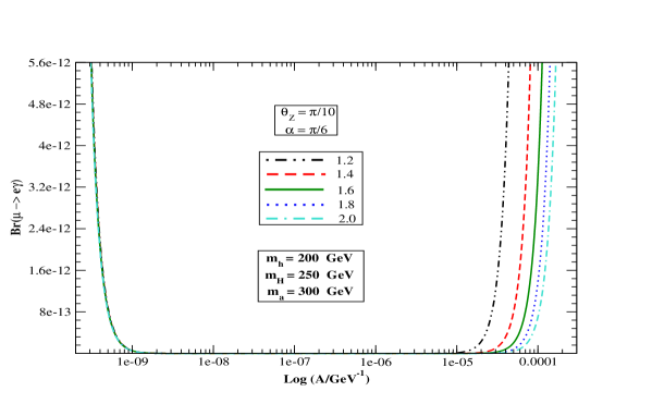
Figure 6: Variations of BR($\mu\rightarrow e\gamma$) with the parameter ”Log A” for different values $(M_{h^{+}_{2}}/M_{h^{+}_{1}})$ ranging from $1.2$ to $2.0$ with $M_{h^{+}_{1}}=250~{}{\rm GeV}$ .

In Fig.-6, to have the desired branching ratio $Br(\mu\rightarrow e\gamma)\sim 10^{-12}$, we see that there are two clearly distinct regions of the parameter $A$ – one for a lower scale of $A\sim 10^{-9}{\rm GeV}^{-1}$ and other in a much higher scale, $A\sim 10^{-4}{\rm GeV}^{-1}$. For the left hand region that means for a relatively lower region of $A$, the coupling constants $f$ are much larger in comparison to $f_{2}$. For example, with the mass ratio equals to 1.4 ( red-dash line) we have the branching ratio $Br(\mu\rightarrow e\gamma)=2.39\times 10^{-12}$ for a value of $A=3.87\times 10^{-10}{\rm GeV}^{-1}$. With this value of $A$, the $f$ coupling constants are given by $f^{e\tau}=0.0249$ and $f^{\mu\tau}=6.34\times 10^{-3}$. However, corresponding $f_{2}$ couplings are much smaller and given by $f_{2}^{\tau e}=-5.43\times 10^{-8}$ and $f_{2}^{\tau\mu}=(1.33+i~{}1.78)\times 10^{-7}$. We see in this lower range, the branching ratio decreases with the increase of $A$ what we can intuitively understand as follows. Note that, here in the lower range of $A$, the main contribution comes from the charged Higgs-sector only, as $f>>f_{2}$. From eqn.(14-16), it is evident that for a fixed set of input parameters the product of $f$ and $A$ is constant. So, an increment of the parameter $A$ reduce the coupling constant $f$ and hence the branching ratio.

On the other hand, for a comparatively large value of $A,\sim 10^{-4}{\rm GeV}^{-1}$, the coupling constants $f_{2}$ has much larger contribution to that of $f$. For example, with the charged scalar mass ratio equals to 1.4 ( red-dash line) we have the branching ratio $Br(\mu\rightarrow e\gamma)=2.21\times 10^{-12}$ for a value of $A=6.43\times 10^{-5}{\rm GeV}^{-1}$. In this case, corresponding different $f_{2}$ coupling constants are given by $f_{2}^{\tau e}=-1.97\times 10^{-3}$ and $f_{2}^{\tau\mu}=(4.83+i~{}6.47)\times 10^{-3}$, while, the much smaller values for the $f$ couplings are given as $f^{e\tau}=1.50\times 10^{-7},f^{\mu\tau}=3.83\times 10^{-8}$.

In this region, the characteristic of the graph is opposite to that at the lower range. The main contribution to the branching ratio comes from $f_{2}$ only. From eqn.(14-16), we see that $f_{2}$ is independent of the parameter $A$. One may, thus, expect a constant value of the branching ratio. However, from eqn.(9), we see the $\rm tan\beta$ is inversely proportional to $A$. Hence, an increment of $A$ implies the increase of the factor $1/\rm tan\beta$, which is appearing in the graphs.

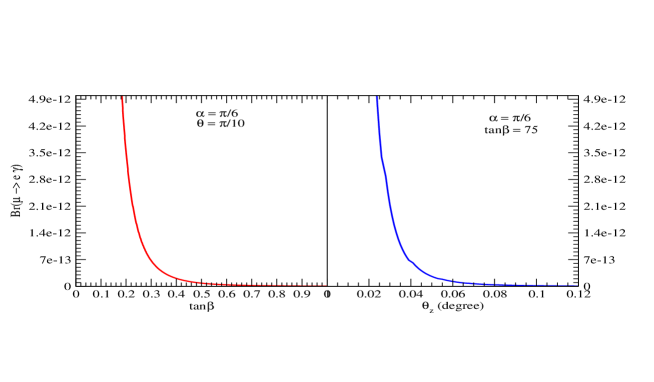
Figure 7: Variations of BR($\mu\rightarrow e\gamma$) with different mixing angles in the charged and neutral Higgs sectors

Since the parameter $A$ depends on the mixing angles as well, to see their impact on the branching ratio, considering the charged scalar mass ratio equals to 1.5, we have shown the variation of BR($\mu\rightarrow e\gamma$) with $\rm tan\beta$ and the mixing angle $\theta_{z}$ in Fig.-7. We see that in either case the branching ratios saturate at their lowest values as the arguments increase.

It is interesting to check if the set of parameters obtained for the $\mu\rightarrow e\gamma$ channel will satisfy other LFV radiative decay processes, namely, $\tau\rightarrow\mu\gamma$ or $\tau\rightarrow e\gamma$ processes. The current experimental limit on the branching ratios of these two decay channels are $Br({\tau\rightarrow\mu\gamma})\leq 2.5\times 10^{-7}$ and $Br({\tau\rightarrow e\gamma})\leq 1.8\times 10^{-7}$ PDG .

In the lower region of $A$ in Fig.-6, where $f^{e\tau},f^{\tau e},f^{\mu\tau}$ and $f^{\tau\mu}$ only significant ones, while $f_{2}$ is negligible, there will not be any significant contribution to the $\tau\to\mu(e)\gamma$ branching ratios. However, had we experimentally observed any of these decay modes we must then analyse the model with corresponding non-zero coupling constants.

On the other hand, for a larger range of $A,\sim 10^{-4}{\rm GeV}^{-1}$, the coupling $f_{2}$ only dominantly contributes to the branching ratio. Here, $f_{2}^{\tau e}$ and $f_{2}^{\tau\mu}$ will open a channel for $\tau$ to radiatively decay into $\mu(e)\gamma$. In Fig.-8, we have shown the variation of the branching ratios with the parameter $A$ for the larger range only. Considering the same set of input parameters we see that the corresponding $\tau$-decay branching ratios can reach to the experimental limit with increase of $A$ for different values of charged scalar mass-ratios.

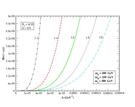
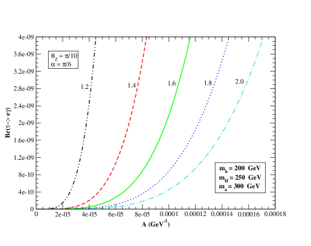
Figure 8: Variations of BR($\tau\rightarrow\mu\gamma$) (left) and BR($\tau\rightarrow e\gamma$) with the parameter ”A” for different set of values $(M_{h^{+}_{2}}/M_{h^{+}_{1}})$ ranging from 1.2 to 2.0.

III.0.2 When both $f$ and $f_{2}$ significantly contribute

Here, we study the parameter space when both the couplings $f$ and $f_{2}$ will have significant contribution to the branching ratio. The parameter space chosen in previous discussion can not lead to MEG result. However, we realise that almost degenerate charged Higgs masses can fullfil the criterion. Variation of the corresponding branching ratio $BR(\mu\to e\gamma)$ is shown on the left panel of Fig.-9 for different values of the charged Higgs scalar mass ratio $(M_{h^{+}_{2}}/M_{h^{+}_{1}})$ ranging from 1.00002 to 1.00010. In this case, other mixing angles as well as the neutral Higgs masses are kept unchanged as like before.

To understand the characteristic of these graphs, we note that in higher range of $A$, the couplings $f_{2}$ is large while $f$ is negligible, and for $A$ of the order of $10^{-10}{\rm GeV}^{-1}$ the case is opposite. It is obvious that for the range of $A\sim{\cal O}(10^{-8}){\rm GeV}^{-1}$, which is almost half-way from two of the above mentioned scale of $A$ in Sec.-III.1, would give same order of values for both the couplings $f$ and $f_{2}$. However, corresponding branching raito is much smaller in magnitude compared to the MEG data. To have the right order of branching ratio $Br(\mu\to e\gamma)$ as shown in the figure, we may have to consider, for example, the resonance effect. In this case two charged Higgs scalars are almost degenerate. For example, with the charged scalar mass ratio equals to 1.00006 ( green-solid line) we have the branching ratio $Br(\mu\rightarrow e\gamma)=2.4\times 10^{-12}$ for a value of $A=4.0\times 10^{-10}{\rm GeV}^{-1}$ and the corresponding different $f_{2}$ coupling constants are given as $f_{2}^{\tau e}=-4.55\times 10^{-4}$ and $f_{2}^{\tau\mu}=(1.12+i~{}1.49)\times 10^{-3}$, while, the $f$ couplings are given by $f^{e\tau}=2.43\times 10^{-2}$ and $f^{\mu\tau}=6.20\times 10^{-3}$. We have seen the same order of magnitude appear once more for the same of charged scalar mass-ratio at a relative larger value of $A$. Here, we see for $A=7.05\times 10^{-9}{\rm GeV}^{-1}$, the branching ratio is $Br(\mu\rightarrow e\gamma)=1.60\times 10^{-12}$.

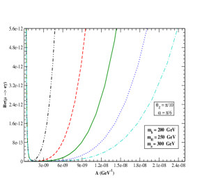
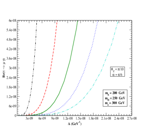
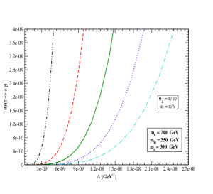
Figure 9: Variations of BR($\mu\rightarrow e\gamma$) (left), BR($\tau\rightarrow\mu\gamma$) (middle) and BR($\tau\rightarrow e\gamma$) (right) with the parameter ”A” for different set of values $(M_{h^{+}_{2}}/M_{h^{+}_{1}})$.

To check, should the same range of $A$ and, hence, coupling constants will allow $\tau$-decay branching ratio to be within the experimental limit, we have shown the variation of both $Br(\tau\rightarrow\mu\gamma)$ or $Br(\tau\rightarrow e\gamma$) on the middle and right panel of Fig.-9. Here, all the parameters are as mentioned above for the $\mu\rightarrow e\gamma$ discussion. We see that both the branching ratios can reach to the experimental limit for the same range of A. For example, with the mass ratio equals to 1.00006 (green-solid line), we have the value of the branching ratio $Br(\tau\rightarrow\mu\gamma)=1.73\times 10^{-8}$ and $Br(\tau\rightarrow e\gamma)=1.02\times 10^{-9}$ for a value of $A=7.05\times 10^{-9}{\rm GeV}^{-1}$.

IV FLAVOUR VIOLATING DECAYS INTO THREE CHARGED LEPTONS ($l_{i}\to l_{j}l_{k}\bar{l}_{l}$)

In this section we discuss the flavour changing charged trilepton decay modes. Recall that in our scenario, nonzero couplings are $f^{e\tau},f^{\mu\tau}$, $f^{\tau e},f^{\tau\mu}$ from $f$ matrix while from $f_{2}$ matrix these are $f_{2}^{\tau e}$ and $f_{2}^{\tau\mu}$ only. These nonzero couplings would induce $l_{i}\to l_{j}l_{k}\bar{l}_{l}$ decay with the exchange of neutral Higgs.

At the tree level, the matrix elements for the $l_{i}\to l_{j}l_{k}\bar{l}_{l}$ decay are given by

$$M_{H} = \frac{1}{m^{2}_{H}}\left(\bar{l}\left[(\frac{\rm cos\alpha}{v\rm sin\beta}m_{E}-\frac{\rm cos(\beta-\alpha)}{\sqrt{2}\rm sin\beta}f^{\dagger}_{2})P_{R}+(\frac{\rm cos\alpha}{v\rm sin\beta}m_{E}-\frac{\rm cos(\beta-\alpha)}{\sqrt{2}\rm sin\beta}f_{2})P_{L}\right]l\right)^{2},$$

$$M_{h} = \frac{1}{m^{2}_{h}}\left(\bar{l}\left[(\frac{\rm sin\alpha}{v\rm sin\beta}m_{E}+\frac{\rm sin(\beta-\alpha)}{\sqrt{2}\rm sin\beta}f^{\dagger}_{2})P_{R}+(\frac{\rm sin\alpha}{v\rm sin\beta}m_{E}+\frac{\rm sin(\beta-\alpha)}{\sqrt{2}\rm sin\beta}f_{2})P_{L}\right]l\right)^{2},$$ (32)

$$M_{a} = \frac{1}{m^{2}_{a}}\left(\bar{l}\left[(\frac{1}{v\rm sin\beta}m_{E}-\frac{1}{\sqrt{2}\rm sin\beta}f^{\dagger}_{2})P_{R}+(\frac{1}{v\rm sin\beta}m_{E}-\frac{1}{\sqrt{2}\rm sin\beta}f_{2})P_{L}\right]l\right)^{2},$$

The $\tau^{-}$ decay width, thus, is given by

$$\Gamma(\tau\rightarrow l\bar{l}j) = \frac{m_{\tau}^{5}}{3072~{}\pi^{3}}\left(|D_{H}+D_{h}+D_{a}|^{2}\right),$$ (33)

where $D_{H/h/a}$ are different contribution to the decay width from respective neutral Higgs scalars. Explicit expressions, for our model, one can read from Appendix-B.

In case, two of the final fermions are identical, the antisymmetrization of the identical fermions and a symmetry factor $1/2$ has to be considered in the formula which lead to an extra-factor $2$ in the numerator.

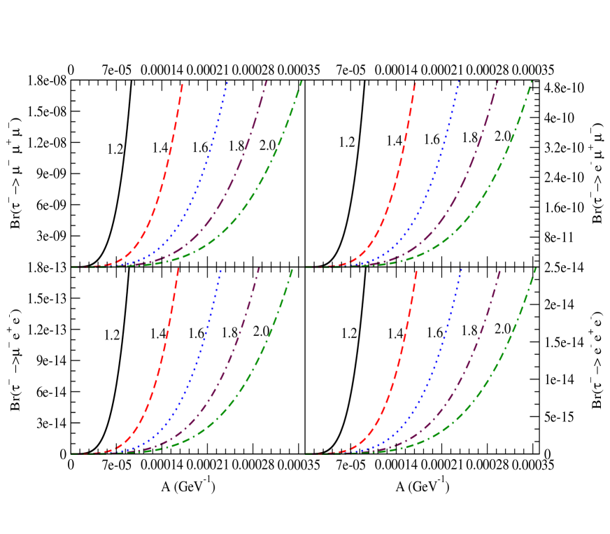
Figure 10: Variations of the branching ratios of different $\tau$ decay modes with the parameter ”A” for different values of $(M_{h^{+}_{2}}/M_{h^{+}_{1}})$.

In Fig.-10, variation of the branching ratio $Br(\tau^{-}\rightarrow\mu^{-}\mu^{+}\mu^{-})$ and $Br(\tau^{-}\rightarrow e^{-}\mu^{+}\mu^{-})$ are shown on the upper row for a set of charged scalar mass ratio, $m_{h^{+}_{2}}/m_{h^{+}_{1}}$, ranging from 1.2 to 2.0, with $m_{h^{+}_{1}}$ set at 250 GeV. The corresponding variations of $Br(\tau^{-}\rightarrow\mu^{-}e^{+}e^{-})$ and $Br(\tau^{-}\rightarrow e^{-}e^{+}e^{-})$ are shown in the lower row. On the top-left figure, we see that the branching ratio $Br(\tau^{-}\rightarrow\mu^{-}\mu^{+}\mu^{-})$ is approaching to the the present experimental limit $<1.8\times 10^{-8}$PDG for the variation of the parameter $A$ upto 0.0002. The rest of the three graphs, within the same range of $A$, are showing the variation of the branching ratios for three other decay modes. For example, from the left-top figure we see that with the mass ratio equals to 1.4 ( red-dash line) we have the branching ratio $Br(\tau^{-}\rightarrow\mu^{-}\mu^{+}\mu^{-})=1.52\times 10^{-8}$ for a value of $A=1.65\times 10^{-4}{\rm GeV}^{-1}$. So, in the same way one can read different coupling constants as before. With the same input parameter $A$, for the branching ratio $Br(\tau^{-}\rightarrow e^{-}e^{+}e^{-})$ the value is, from right bottom figure, $2.11\times 10^{-14}$, as expected from the electron to muon mass-squared ratios. The corresponding values for $Br(\tau^{-}\rightarrow e^{-}\mu^{+}\mu^{-})$ and $Br(\tau^{-}\rightarrow\mu^{-}e^{+}e^{-})$ are given by $4.52\times 10^{-10}$ and $1.78\times 10^{-13}$ respectively. In the analysis, we see that the $Br(\tau\to\mu\mu\bar{\mu})$ is the largest one, equals $\sim 10^{-8}$ for a value of $A\sim 10^{-4}{\rm GeV}^{-1}$. The same value of $A$ and other input parameters we see that to other charged tri-leptons decay modes branching ratios are suppressed by the electron to muon mass ratio or it’s higher power depending on the number of electron and muon in final states.

The trilepton $\mu$ decay mode $(\mu^{-}\to e^{-}e^{+}e^{-})$, at tree level, does not exist as it depends on the coupling constants $f_{2}^{\mu e}$. However, to add, we have to consider a scenario with a nonzero $f_{2}^{\mu e}$ if we have any experimental evidence of muon decaying to three charged leptons process.

V CONCLUSIONS AND Discussions

Observation of neutrino oscillations, and hence neutrino masses, is one of the main evidence to look into beyond the standard model. Understanding of the smallness of neutrino masses requires new physics, such as loop induced masses as in the Zee model. These models do allow some processes which violate lepton flavour. There are strong experimental constraints on LFV interaction. Recently MEG collaboration has report a new upper bound of $2.4\times 10^{-12}$ for $\mu\to e\gamma$ branching ratio. This improved upper bound may have implications on models for neutrino mass and mixing. On the other hand, the recent data from T2K, MINOS and Double Chooz provide some new information on the mixing angles in $V_{PMNS}$ that the last mixing angle $\theta_{13}$ is non-zero at more than 2$\sigma$ level. The combined data analysis gives the confidence level at more than 3$\sigma$.

In the simplest Zee model, the mass matrix has all diagonal entries to be zero. This type of mass matrix has been shown to be ruled out. This is basically because that it cannot simultaneously have solution for $|V_{\mu 3}|$ close to $1/\sqrt{2}$ and $|V_{e2}|$ close to $1/\sqrt{3}$ as data require.

In this article, it has been proposed that an interesting mass matrix can result if one imposes the requirement that no large hierarchies among the new couplings, that is, all nonzero $f^{ij}$ and $f^{ij}_{2}$ are of the same order of magnitude, respectively. This will lead to mass-matrix where all the elements are either proportional to the charged lepton mass or to it’s square. A few important outcome in the neutrino section of the model are the following:-

• The model is constraint to have a non-zero $\theta_{13}$, which is in consistent with the present experimental data.

• The best-fit value of our model predicts for $\theta_{13}$ equals to $8.91^{\circ}$ which is close to the recent data from Double Chooz.

• Existence of solutions for non-zero CP violation with the Jarlskog parameter predicted in the range $\pm 0.039$, $\pm 0.044$ and $\pm 0.048$ respectively for a 1$\sigma$, 2$\sigma$ and 3$\sigma$ ranges of neutrino masses and mixing angles. However, lifting the constraints on $\theta_{13}$ the above respective ranges become $\pm 0.049$, $\pm 0.053$ and $\pm 0.056$.

For the inverted hierarchy only, the best-fit values of the mass matrix parameters are:

$$x = 0.255,~{}~{}~{}y=4.100,~{}~{}~{}z=1.790,~{}~{}~{}a=0.017~{}{\rm eV},~{}~{}~{}\delta=180^{\circ},$$

and, the corresponding output for the mixing angles and mass-squared differences are given as follows

$$~{}~{}{\rm sin}^{2}\theta_{12}=0.3163,~{}~{}{\rm sin}^{2}\theta_{23}=0.4033,~{}~{}{\rm sin}^{2}\theta_{13}=0.0256,$$

$$~{}~{}\delta m^{2}=7.51\times 10^{-5}{\rm eV^{2}}~{}~{}\Delta m^{2}=-2.36\times 10^{-3}{\rm eV^{2}}.$$

We have also discussed if these best-fit values satisfy different constraints for the lepton flavour violating processes. In that direction we have considered the radiative decay processes like $\mu\to e\gamma$ and $\tau\to\mu(e)\gamma$ processes and the decay modes to three charged leptons $\tau^{-}\to\mu^{-}\mu^{+}\mu^{-}$, $\tau^{-}\to e^{-}\mu^{+}\mu^{-}$, $\tau^{-}\to\mu^{-}e^{+}e^{-}$ and $\tau^{-}\to e^{-}e^{+}e^{-}$ processes. Here, we look into that range of parameter space which will lead to the experimental limit of these decay modes, for example, the constraints set by the MEG collaboration for the $\mu\to e\gamma$ process.

To have a better understanding on how different parameters contribute to the branching ratios we have discussed different cases – when either of the coupling constants $f_{2}$ or $f$ has a dominant contribution and when both the couplings $f$ and $f_{2}$ have comparable contributions to different $\mu$ and $\tau$-radiative decay modes.

We have extensively shown how these different cases correspond to various ranges of the parameter $A$, and hence the set of non-zero coupling constants, to have a branching ratio close or within the experimental limit.

There are a pair of charged Higgs bosons, two CP-even and one CP-odd neutral Higgs bosons in the Zee model. The Higgs sector is just enriched by one more charged scalar component than the Two Higgs doublet model. The collider phenomenology of Higgs sector in the Zee model is studied in various literature, for example Kanemura:2000bq . A very well known way to analyse this model at LHC, is the pair production of charged and neutral Higgs via Drell-Yan process. Different decay modes of these Higgs bosons will lead to multi-lepton plus missing energy topology in the final states. However, depending on the coupling constants and mass of the neutral Higgs boson various channel, like decaying to di-photon, will be modified. How different channels are affected due to our model specific coupling constant parameter space will be separately discussed in future.

Within the allowed non-zero parameter space, the only possible lepton flavour violating decay modes in our model are $\mu\to e\gamma$, $\tau\to\mu(e)\gamma$, $\tau\to\mu(\mu\bar{\mu},e\bar{e})$ and $\tau\to e(\mu\bar{\mu},e\bar{e})$. Collider search of lepton-flavour violating decay modes is a clear signal to hunt for beyond the SM. A large number of past as well as recent articles have already studied this LFV. In our analysis, we see that the $Br(\tau\to\mu\mu\bar{\mu})$ is the largest one, equals $\sim 10^{-8}$ for a value of $A\sim 10^{-4}{\rm GeV}^{-1}$. Not only a relatively large branching ratio but muons are favourable for their clear signal at LHC. We would thus be interested here for the decay channel $\tau\to\mu\mu\bar{\mu}$ mediated via different neutral scalars. At LHC, the main contribution to the production of $\tau$-lepton via the heavy meson $B$ or $D$ decays and weak $W$ and $Z$ gauge bosons. Recently, LHC acquired a total integrated luminosity of 5 $fb^{-1}$ per year. We will consider this analysis in a future work hm2 in detail.

Appendix A Higgs Scalars Contribution to Radiative LFV Decays

In this appendix, we write down the explicit expression of $C_{L}$ and $C_{R}$ due to the charged scalars, $h_{1}^{+},h_{2}^{+}$, and neutral scalars, $H,h,{\rm a}$. These two factors $C_{L}$ and $C_{R}$ can be written as

$$C_{L} = \frac{1}{16\pi^{2}}\left\{Q_{S}(C_{h_{1}^{+}}+C_{h_{2}^{+}})-Q_{f}(C_{H}+C_{h}+C_{a})\right\},$$ (34)

where, $Q_{S}=-1$ is the charge of $h^{-}_{i}$ and $Q_{f}=-1$ is the charge of charged lepton, while $C_{R}=C_{L}^{\dagger}$.

The matrix $C_{L}$ is given by

$$C_{h_{1}^{+}} = \begin{pmatrix}\frac{\sqrt{2}}{v\rm tan\beta}m_{E}-\frac{1}{\rm sin\beta}f_{2}\end{pmatrix}\tilde{F}_{2}(z_{h_{1}})\begin{pmatrix}\frac{\sqrt{2}}{v\rm tan\beta}m_{E}-\frac{1}{\rm sin\beta}{f_{2}^{\dagger}}\end{pmatrix}m_{E}\frac{{\rm sin}^{2}\theta}{m^{2}_{h^{+}_{1}}}+4m_{E}{f^{\dagger}}\tilde{F}_{2}(z_{h_{1}})f\frac{{\rm cos}^{2}\theta}{m^{2}_{h^{+}_{1}}},$$ (35)

$$C_{h_{2}^{+}} = \begin{pmatrix}\frac{\sqrt{2}}{v\rm tan\beta}m_{E}-\frac{1}{\rm sin\beta}f_{2}\end{pmatrix}\tilde{F}_{2}(z_{h_{2}})\begin{pmatrix}\frac{\sqrt{2}}{v\rm tan\beta}m_{E}-\frac{1}{\rm sin\beta}{f_{2}^{\dagger}}\end{pmatrix}m_{E}\frac{{\rm cos}^{2}\theta}{m^{2}_{h^{+}_{2}}}+4m_{E}{f^{\dagger}}\tilde{F}_{2}(z_{h_{2}})f\frac{{\rm sin}^{2}\theta}{m^{2}_{h^{+}_{2}}},$$ (36)

$$C_{H} = \bigg{[}\begin{pmatrix}\frac{\rm cos\alpha}{v\rm sin\beta}m_{E}-\frac{\rm cos(\beta-\alpha)}{\sqrt{2}\rm sin\beta}f_{2}^{\dagger}\end{pmatrix}\tilde{F}_{1}(z_{H})\begin{pmatrix}\frac{\rm cos\alpha}{v\rm sin\beta}m_{E}-\frac{\rm cos(\beta-\alpha)}{\sqrt{2}\rm sin\beta}f_{2}\end{pmatrix}m_{E}$$

$$~{}+m_{E}\begin{pmatrix}\frac{\rm cos\alpha}{v\rm sin\beta}m_{E}-\frac{\rm cos(\beta-\alpha)}{\sqrt{2}\rm sin\beta}f_{2}\end{pmatrix}\tilde{F}_{1}(z_{H})\begin{pmatrix}\frac{\rm cos\alpha}{v\rm sin\beta}m_{E}-\frac{\rm cos(\beta-\alpha)}{\sqrt{2}\rm sin\beta}f_{2}^{\dagger}\end{pmatrix}$$

$$+\begin{pmatrix}\frac{\rm cos\alpha}{v\rm sin\beta}m_{E}-\frac{\rm cos(\beta-\alpha)}{\sqrt{2}\rm sin\beta}f_{2}\end{pmatrix}m_{E}\tilde{F}_{3}(z_{H})\begin{pmatrix}\frac{\rm cos\alpha}{v\rm sin\beta}m_{E}-\frac{\rm cos(\beta-\alpha)}{\sqrt{2}\rm sin\beta}{f_{2}}\end{pmatrix}\bigg{]}\frac{1}{m^{2}_{H}},$$

$$C_{h} = \bigg{[}\begin{pmatrix}\frac{\rm sin\alpha}{v\rm sin\beta}m_{E}+\frac{\rm sin(\beta-\alpha)}{\sqrt{2}\rm sin\beta}f_{2}^{\dagger}\end{pmatrix}\tilde{F}_{1}(z_{h})\begin{pmatrix}\frac{\rm sin\alpha}{v\rm sin\beta}m_{E}+\frac{\rm sin(\beta-\alpha)}{\sqrt{2}\rm sin\beta}f_{2}\end{pmatrix}m_{E}$$

$$~{}+m_{E}\begin{pmatrix}\frac{\rm sin\alpha}{v\rm sin\beta}m_{E}+\frac{\rm sin(\beta-\alpha)}{\sqrt{2}\rm sin\beta}f_{2}\end{pmatrix}\tilde{F}_{1}(z_{h})\begin{pmatrix}\frac{\rm sin\alpha}{v\rm sin\beta}m_{E}+\frac{\rm sin(\beta-\alpha)}{\sqrt{2}\rm sin\beta}f_{2}^{\dagger}\end{pmatrix}$$

$$+\begin{pmatrix}\frac{\rm sin\alpha}{v\rm sin\beta}m_{E}+\frac{\rm sin(\beta-\alpha)}{\sqrt{2}\rm sin\beta}f_{2}\end{pmatrix}m_{E}\tilde{F}_{3}(z_{h})\begin{pmatrix}\frac{\rm sin\alpha}{v\rm sin\beta}m_{E}+\frac{\rm sin(\beta-\alpha)}{\sqrt{2}\rm sin\beta}{f_{2}}\end{pmatrix}\bigg{]}\frac{1}{m^{2}_{h}},$$

$$C_{a} = \bigg{[}\begin{pmatrix}\frac{1}{v\rm tan\beta}m_{E}-\frac{1}{\sqrt{2}\rm sin\beta}f_{2}^{\dagger}\end{pmatrix}\tilde{F}_{1}(z_{a})\begin{pmatrix}\frac{1}{v\rm tan\beta}m_{E}-\frac{1}{\sqrt{2}\rm sin\beta}f_{2}\end{pmatrix}m_{E}$$

$$~{}+m_{E}\begin{pmatrix}\frac{1}{v\rm tan\beta}m_{E}-\frac{1}{\sqrt{2}\rm sin\beta}f_{2}\end{pmatrix}\tilde{F}_{1}(z_{a})\begin{pmatrix}\frac{1}{v\rm tan\beta}m_{E}-\frac{1}{\sqrt{2}\rm sin\beta}f_{2}^{\dagger}\end{pmatrix}$$

$$+\begin{pmatrix}\frac{1}{v\rm tan\beta}m_{E}-\frac{1}{\sqrt{2}\rm sin\beta}f_{2}\end{pmatrix}m_{E}\tilde{F}_{3}(z_{a})\begin{pmatrix}\frac{1}{v\rm tan\beta}m_{E}-\frac{1}{\sqrt{2}\rm sin\beta}{f_{2}}\end{pmatrix}\bigg{]}\frac{1}{m^{2}_{a}}.$$

In the above equations $\tilde{F}_{\alpha}(z_{i})$ is a diagonal matrix $\tilde{F}_{\alpha}(z_{i})=diag(F_{\alpha}(z_{1}),F_{\alpha}(z_{2}),F_{\alpha}(z_{3}))$, where $z_{i}=m_{i}^{2}/m_{S}^{2}$ with $m_{i}$ the fermion “i” mass and scalar “S” in the loop, respectively.

The functions $F_{1}(z),F_{2}(z){~{}\rm and~{}}F_{3}(z)$ are given by

$$F_{1}(z)=\frac{z^{2}-5z-2}{12(z-1)^{3}}+\frac{z\ln z}{2(z-1)^{4}}\;,\;\;$$

$$F_{2}(z)=\frac{2z^{2}+5z-1}{12(z-1)^{3}}-\frac{z^{2}\ln z}{2(z-1)^{4}}\;,$$

$$F_{3}(z)=\frac{z-3}{2(z-1)^{2}}+\frac{\ln z}{(z-1)^{3}}\;.\;\;$$ (40)

To be noted here, in the limit $z\rightarrow 0$ both the functions $F_{1}(z)$ and $F_{2}(z)$ do not any more depend on the argument of the functions, and take finite values $-1/6$ and $-1/12$ respectively. On the other hand, the characteristic of the function $F_{3}(z)$ is different and goes as $\ln z$ in the limit $z\rightarrow 0$. However, the final expressions for $C_{L,R}$ are finite in the limit $z\rightarrow 0$.

Appendix B Neutral Higgs scalar contribution to $\tau\to l_{1}l_{2}\bar{l}_{3}$

Here, we will explicitly show different neutral scalar contribution to the lepton flavour violating trilepton decay mode of $\tau$-decays in our model. With the non-zero $f$ and $f_{2}$ we are considering, we find only, $\tau\to\mu(\mu\bar{\mu},e\bar{e})$ and $\tau\to e(\mu\bar{\mu},e\bar{e})$.

The matrix elements are of the form: $M=D_{\alpha}\bar{l}l\bar{j}P_{R}\tau$ with $D_{\alpha}$ given by for different processes and different Higgs $\alpha$ contributions

$$\tau\to\mu\mu\bar{\mu}: D_{H}=-\frac{1}{m^{2}_{H}}\frac{\rm cos\alpha}{v\rm sin\beta}\frac{\rm cos(\beta-\alpha)}{\sqrt{2}\rm sin\beta}m_{\mu}f_{2}^{\tau\mu*},$$

$$D_{h}=\frac{1}{m^{2}_{h}}\frac{\rm sin\alpha}{v\rm sin\beta}\frac{\rm sin(\beta-\alpha)}{\sqrt{2}\rm sin\beta}m_{\mu}f_{2}^{\tau\mu*},$$

$$D_{a}=-\frac{1}{m^{2}_{a}}\frac{1}{v\rm sin\beta}\frac{1}{\sqrt{2}\rm sin\beta}m_{\mu}f_{2}^{\tau\mu*},$$

$$\tau\to e\mu\bar{\mu}: D_{H}=-\frac{1}{m^{2}_{H}}\frac{\rm cos\alpha}{v\rm sin\beta}\frac{\rm cos(\beta-\alpha)}{\sqrt{2}\rm sin\beta}m_{\mu}f_{2}^{\tau e*},$$

$$D_{h}=\frac{1}{m^{2}_{h}}\frac{\rm sin\alpha}{v\rm sin\beta}\frac{\rm sin(\beta-\alpha)}{\sqrt{2}\rm sin\beta}m_{\mu}f_{2}^{\tau e*},$$

$$D_{a}=-\frac{1}{m^{2}_{a}}\frac{1}{v\rm sin\beta}\frac{1}{\sqrt{2}\rm sin\beta}m_{\mu}f_{2}^{\tau e*},$$

$$\tau\to\mu e\bar{e}: D_{H}=-\frac{1}{m^{2}_{H}}\frac{\rm cos\alpha}{v\rm sin\beta}\frac{\rm cos(\beta-\alpha)}{\sqrt{2}\rm sin\beta}m_{e}f_{2}^{\tau\mu*},$$

$$D_{h}=\frac{1}{m^{2}_{h}}\frac{\rm sin\alpha}{v\rm sin\beta}\frac{\rm sin(\beta-\alpha)}{\sqrt{2}\rm sin\beta}m_{e}f_{2}^{\tau\mu*},$$

$$D_{a}=-\frac{1}{m^{2}_{a}}\frac{1}{v\rm sin\beta}\frac{1}{\sqrt{2}\rm sin\beta}m_{e}f_{2}^{\tau\mu*},$$

$$\tau\to ee\bar{e}: D_{H}=-\frac{1}{m^{2}_{H}}\frac{\rm cos\alpha}{v\rm sin\beta}\frac{\rm cos(\beta-\alpha)}{\sqrt{2}\rm sin\beta}m_{e}f_{2}^{\tau e*},$$

$$D_{h}=\frac{1}{m^{2}_{h}}\frac{\rm sin\alpha}{v\rm sin\beta}\frac{\rm sin(\beta-\alpha)}{\sqrt{2}\rm sin\beta}m_{e}f_{2}^{\tau e*},$$

$$D_{a}=-\frac{1}{m^{2}_{a}}\frac{1}{v\rm sin\beta}\frac{1}{\sqrt{2}\rm sin\beta}m_{e}f_{2}^{\tau e*}.$$

References

-
(1)
Z. Maki, M. Nakagawa, and S. Sakata,
“Remarks on the unified model of elementary particles,”
Prog. Theor. Phys. 28, 870 (1962);
B. Pontecorvo, “Neutrino experiments and the question of leptonic-charge conservation,” Sov. Phys. JETP 26 (1968) 984 [Zh. Eksp. Teor. Fiz. 53 (1967) 1717].
-
(2)
A. Zee,
“A Theory of Lepton Number Violation, Neutrino Majorana Mass, and
Oscillation,”
Phys. Lett. B93, 389 (1980)
[Erratum-ibid. B95, 461 (1980)].
-
(3)
P. Minkowski,
“Mu E Gamma At A Rate Of One Out Of 1-Billion Muon Decays?,”
Phys. Lett. B67 (1977) 421;
M. Gell-Mann, P. Ramond and R. Slansky,
“Complex Spinors And Unified Theories,”
Proceedings of the Supergravity Stony Brook Workshop, eds. P. van Niewenhuizen and
D. Freedman (New York, 1979);
T. Yanagida,
“Horizontal gauge symmetry and masses of neutrinos,”
SPIRES entry
Proceedings of the Workshop on the Baryon Number of the Universe and Unified Theories,
Tsukuba, Japan, 13-14 Feb 1979;
R. N. Mohapatra and G. Senjanovic,
“Neutrino mass and spontaneous parity nonconservation,”
Phys. Rev. Lett. 44, 912 (1980) .
-
(4)
M. Magg and C. Wetterich,
“Neutrino Mass Problem And Gauge Hierarchy,”
Phys. Lett. B94, 61 (1980);
T. P. Cheng and L. F. Li,
“Neutrino Masses, Mixings And Oscillations In SU(2) X U(1) Models Of
Electroweak Interactions,”
Phys. Rev. D22, 2860 (1980);
G. B. Gelmini and M. Roncadelli,
“Left-Handed Neutrino Mass Scale And Spontaneously Broken Lepton Number,”
Phys. Lett. B99, 411 (1981);
G. Lazarides, Q. Shafi and C. Wetterich,
“Proton Lifetime And Fermion Masses In An SO(10) Model,”
Nucl. Phys. B181, 287 (1981) ;
R. N. Mohapatra and G. Senjanovic,
“Neutrino Masses And Mixings In Gauge Models With Spontaneous Parity
Violation,”
Phys. Rev. D23, 165 (1981);
J.Schechter and J.W.F. Valle, Phys. ReV. D22, 2227, (1980);
E. Ma and U. Sarkar,
“Neutrino masses and leptogenesis with heavy Higgs triplets,”
Phys. Rev. Lett. 80, 5716 (1998)
[arXiv:hep-ph/9802445].
-
(5)
R. Foot, H. Lew, X. G. He and G. C. Joshi,
“Seesaw Neutrino Masses Induced By A Triplet Of Leptons,”
Z. Phys. C44, 441 (1989);
E. Ma,
“Pathways to naturally small neutrino masses,”
Phys. Rev. Lett. 81, 1171 (1998)
[hep-ph/9805219] .
-
(6)
K. Nakamura et al. [ Particle Data Group Collaboration ],
“Review of particle physics,”
J. Phys. G37, 075021 (2010).
-
(7)
S. T. Petcov,
“Remarks on the Zee Model of Neutrino Mixing (, Heavy Neutrino Light Neutrino , etc.),” Phys. Lett. B115, 401-406 (1982);
U. Sarkar,
“17-keV neutrino in a Zee type model and SU(5) GUT,”
Phys. Rev. D47, 1114-1116 (1993);
A. Y. .Smirnov, Z. -j. Tao,
“Neutrinos with Zee mass matrix in vacuum and matter,”
Nucl. Phys. B426, 415-433 (1994)
[hep-ph/9403311];
A. Y. .Smirnov, M. Tanimoto,
“Is Zee model the model of neutrino masses?,”
Phys. Rev. D55, 1665-1671 (1997) [hep-ph/9604370];
K. S. Babu,
“Model of ’Calculable’ Majorana Neutrino Masses,”
Phys. Lett. B203, 132 (1988);
C. Jarlskog, M. Matsuda, S. Skadhauge, M. Tanimoto,
“Zee mass matrix and bimaximal neutrino mixing,”
Phys. Lett. B449, 240 (1999) [hep-ph/9812282];
P. H. Frampton, S. L. Glashow,
“Can the Zee ansatz for neutrino masses be correct?,”
Phys. Lett. B461, 95-98 (1999) [hep-ph/9906375];
A. S. Joshipura, S. D. Rindani,
“Neutrino anomalies in an extended Zee model,”
Phys. Lett. B464, 239-243 (1999) [hep-ph/9907390];
G. C. McLaughlin, J. N. Ng,
“Singlet interacting neutrinos in the extended Zee model and solar neutrino transformation,”
Phys. Lett. B464, 232-238 (1999) [hep-ph/9907449];
K. -m. Cheung, O. C. W. Kong,
“Zee neutrino mass model in SUSY framework,”
Phys. Rev. D61, 113012 (2000) [hep-ph/9912238];
D. Chang, A. Zee,
“Radiatively induced neutrino Majorana masses and oscillation,”
Phys. Rev. D61, 071303 (2000) [hep-ph/9912380];
D. A. Dicus, H. -J. He, J. N. Ng,
“Neutrino - lepton masses, Zee scalars and muon g-2,”
Phys. Rev. Lett. 87, 111803 (2001) [hep-ph/0103126];
K. R. S. Balaji, W. Grimus, T. Schwetz,
“The Solar LMA neutrino oscillation solution in the Zee model,”
Phys. Lett. B508, 301-310 (2001) [hep-ph/0104035];
E. Mitsuda, K. Sasaki,
“Zee model and phenomenology of lepton sector,”
Phys. Lett. B516, 47-53 (2001);
A. Ghosal, Y. Koide, H. Fusaoka,
“Lepton flavor violating Z decays in the Zee model,”
Phys. Rev. D64, 053012 (2001) [hep-ph/0104104];
Y. Koide,
“Can the Zee model explain the observed neutrino data?,”
Phys. Rev. D64, 077301 (2001) [hep-ph/0104226];
B. Brahmachari, S. Choubey,
“Viability of bimaximal solution of the Zee mass matrix,”
Phys. Lett. B531, 99-104 (2002) [hep-ph/0111133];
T. Kitabayashi, M. Yasue,
“Large solar neutrino mixing in an extended Zee model,”
Int. J. Mod. Phys. A17, 2519-2534 (2002) [hep-ph/0112287];
Y. Koide,
“Prospect of the Zee model,”
Nucl. Phys. Proc. Suppl. 111, 294-296 (2002) [hep-ph/0201250];
M. -Y. Cheng, K. -m. Cheung,
“Zee model and neutrinoless double beta decay,” [hep-ph/0203051];
X. G. He, A. Zee,
“Some simple mixing and mass matrices for neutrinos,”
Phys. Lett. B560, 87-90 (2003) [hep-ph/0301092];
K. Hasegawa, C. S. Lim, K. Ogure,
“Escape from washing out of baryon number in a two zero texture general Zee model compatible with the LMA-MSW solution,”
Phys. Rev. D68, 053006 (2003) [hep-ph/0303252];
S. Kanemura, T. Ota, K. Tsumura,
“Lepton flavor violation in Higgs boson decays under the rare tau
decay results,”
Phys. Rev. D73, 016006 (2006) [arXiv:hep-ph/0505191 [hep-ph]];
D. Aristizabal Sierra, D. Restrepo,
“Leptonic Charged Higgs Decays in the Zee Model,”
JHEP 0608, 036 (2006) [hep-ph/0604012];
B. Brahmachari, S. Choubey,
“Modified Zee mass matrix with zero-sum condition,”
Phys. Lett. B642, 495-502 (2006) [hep-ph/0608089];
N. Sahu, U. Sarkar,
“Extended Zee model for Neutrino Mass, Leptogenesis and Sterile Neutrino like Dark Matter,”
Phys. Rev. D78, 115013 (2008) [arXiv:0804.2072 [hep-ph]];
T. Fukuyama, H. Sugiyama, K. Tsumura,
“Phenomenology in the Zee Model with the Symmetry,”
Phys. Rev. D83, 056016 (2011) [arXiv:1012.4886 [hep-ph]].
-
(8)
K. Abe et al. [T2K Collaboration],
“Indication of Electron Neutrino Appearance from an Accelerator-produced
Off-axis Muon Neutrino Beam,”
Phys. Rev. Lett. 107, 041801 (2011)
[arXiv:1106.2822 [hep-ex]].
-
(9)
P. Adamson et al. [MINOS Collaboration],
“Improved search for muon-neutrino to electron-neutrino oscillations in
MINOS,”
arXiv:1108.0015 [hep-ex].
-
(10)
Double Chooz, H. D. Kerret, (2011), LowNu2011, 9-12,
November, 2011, Seoul National University, Seoul, Korea.
-
(11)
G. Bhattacharyya, H. Pas and D. Pidt,
“R-Parity violating flavor symmetries, recent neutrino data and absolute
neutrino mass scale,”
arXiv:1109.6183 [hep-ph];
S. -F. Ge, D. A. Dicus and W. W. Repko,
“ Symmetry Prediction for the Leptonic Dirac CP Phase,”
Phys. Lett. B 702 (2011) 220
[arXiv:1104.0602 [hep-ph]].
S. -F. Ge, D. A. Dicus and W. W. Repko,
“Residual Symmetries for Neutrino Mixing with a Large and Nearly Maximal ,”
arXiv:1108.0964 [hep-ph].
T. Araki, C. -Q. Geng,
“Large from finite quantum corrections in quasi-degenerate neutrino mass spectrum,”
JHEP 1109, 139 (2011) [arXiv:1108.3175 [hep-ph]];
R. N. Mohapatra, M. K. Parida,
“Type II Seesaw Dominance in Non-supersymmetric and Split Susy SO(10) and Proton Life Time,”
[arXiv:1109.2188 [hep-ph]];
A. Rashed, A. Datta,
“The charged lepton mass matrix and non-zero with TeV scale New Physics,”
[arXiv:1109.2320 [hep-ph]];
N. Okada, Q. Shafi,
“, CP Violation and Leptogenesis in Minimal Supersymmetric ,”
[arXiv:1109.4963 [hep-ph]];
S. K. Agarwalla, T. Li and A. Rubbia,
“An incremental approach to unravel the neutrino mass hierarchy and CP
violation with a long-baseline Superbeam for large ,”
arXiv:1109.6526 [hep-ph];
N. Haba, T. Horita, K. Kaneta, Y. Mimura,
“TeV-scale seesaw with non-negligible left-right neutrino mixings,”
[arXiv:1110.2252 [hep-ph]];
A. Dighe, S. Goswami, S. Ray,
“Optimization of the baseline and the parent muon energy for a low energy neutrino factory,”
[arXiv:1110.3289 [hep-ph]].
-
(12)
J. Adam et al. [MEG collaboration],
“New limit on the lepton-flavour violating decay ,”
arXiv:1107.5547 [hep-ex].
-
(13)
X. -G. He,
“Is the Zee model neutrino mass matrix ruled out?,”
Eur. Phys. J. C34, 371-376 (2004).
[hep-ph/0307172];
Y. Koide,
“Prospect of the Zee model,”
Nucl. Phys. Proc. Suppl. 111, 294 (2002)
[arXiv:hep-ph/0201250];
P. H. Frampton, M. C. Oh, T. Yoshikawa,
“Zee model confronts SNO data,”
Phys. Rev. D65, 073014 (2002).
[hep-ph/0110300].
-
(14)
G. L. Fogli, E. Lisi, A. Marrone, A. Palazzo, A. M. Rotunno,
“Evidence of from global neutrino data analysis,”
[arXiv:1106.6028 [hep-ph]].
-
(15)
T. Schwetz, M. Tortola and J. W. F. Valle,
“Where we are on : addendum to ’Global neutrino data and recent reactor fluxes: status of three-flavour oscillation parameters’,”
New J. Phys. 13 (2011) 109401
[arXiv:1108.1376 [hep-ph]].
-
(16)
R. Brugnera [GERDA Collaboration],
“Search for neutrinoless double beta decay of Ge-76 with the GERmanium Detector Array ’GERDA’,”
PoS EPS -HEP2009 (2009) 273.
-
(17)
D. G. Phillips, II, E. Aguayo, F. T. Avignone, III, H. O. Back, A. S. Barabash, M. Bergevin, F. E. Bertrand and M. Boswell et al.,
“The Majorana experiment: an ultra-low background search for neutrinoless double-beta decay,”
arXiv:1111.5578 [nucl-ex].
-
(18)
M. Gunther et al.,
“Heidelberg - Moscow beta beta experiment with Ge-76: Full setup with five
detectors,”
Phys. Rev. D 55 (1997) 54,
L. Baudis et al.,
“The Heidelberg - Moscow Experiment: Improved sensitivity for Ge-76
neutrinoless double beta decay,”
Phys. Lett. B 407 (1997) 219,
L. Baudis et al.,
“Limits on the Majorana neutrino mass in the 0.1 eV range,”
Phys. Rev. Lett. 83 (1999) 41
[arXiv:hep-ex/9902014],
H. V. Klapdor-Kleingrothaus et al.,
“Latest Results from the Heidelberg-Moscow Double Beta Decay Experiment,”
Eur. Phys. J. A 12 (2001) 147
[arXiv:hep-ph/0103062],
H. V. Klapdor-Kleingrothaus, A. Dietz, H. L. Harney and I. V. Krivosheina,
“Evidence for Neutrinoless Double Beta Decay,”
Mod. Phys. Lett. A 16 (2001) 2409
[arXiv:hep-ph/0201231].
H. V. Klapdor-Kleingrothaus, I. V. Krivosheina, A. Dietz and O. Chkvorets,
“Search for neutrinoless double beta decay with enriched in Gran Sasso 1990-2003,”
Phys. Lett. B 586 (2004) 198
[hep-ph/0404088].
-
(19)
L. Lavoura,
“General formulae for ,”
Eur. Phys. J. C29, 191-195 (2003).
[hep-ph/0302221].
-
(20)
S. Kanemura, T. Kasai, G. -L. Lin, Y. Okada, J. -J. Tseng and C. P. Yuan,
“Phenomenology of Higgs bosons in the Zee model,”
Phys. Rev. D 64 (2001) 053007
[hep-ph/0011357];
K. A. Assamagan, A. Deandrea and P. -A. Delsart,
“Search for the lepton flavor violating decay at hadron colliders,”
Phys. Rev. D 67 (2003) 035001
[hep-ph/0207302].
- (21) Xiao-Gang He, Swarup Kumar Majee, in preparation.