Quasi-particle Statistics and Braiding from Ground State Entanglement

Abstract

Topologically ordered phases are gapped states, defined by the properties of excitations when taken around one another. Here we demonstrate a method to extract the statistics and braiding of excitations, given just the set of ground-state wave functions on a torus. This is achieved by studying the Topological Entanglement Entropy (TEE) on partitioning the torus into two cylinders. In this setting, general considerations dictate that the TEE generally differs from that in trivial partitions and depends on the chosen ground state. Central to our scheme is the identification of ground states with minimum entanglement entropy, which reflect the quasi-particle excitations of the topological phase. The transformation of these states allows for a determination of the modular $\mathcal{S}$ and $\mathcal{U}$ matrices which encode quasi-particle properties. We demonstrate our method by extracting the modular $\mathcal{S}$ matrix of a SU(2) spin symmetric chiral spin liquid phase using a Monte Carlo scheme to calculate TEE, and prove that the quasi-particles obey semionic statistics. This method offers a route to a nearly complete determination of the topological order in certain cases.

I Introduction

Topologically ordered states are exotic gapped quantum phases of matter that lie beyond the Landau symmetry breaking paradigm wen2004 . Well known examples include fractional quantum Hall states, gapped quantum spin liquids and quantum dimer models wen2004 ; anderson1987 ; wen1990 ; Read89 ; wen1991 ; read1991 ; senthil2000 ; sondhi . These phases are not characterized by correlations or local order parameters but rather by long range entanglement in their ground-state wave functions kitaev2003 . Emergent excitations in these phases can carry fractional quantum numbers and, in two dimensions, realize non-trivial statistics on exchanging identical particles or on taking one particle type around another nayak . Two important hallmarks of topologically ordered phases are ground-state degeneracy in a space with non-zero genus and a finite topological entanglement entropy (TEE) hamma2005 ; kitaev2006 ; levin2006 . In this paper we show that combined together, these two properties can be used to extract key aspects of a topological phase such as braiding rules and topological spin of quasi-particlesnayak .

Taking a more general perspective, we note that a gapped phase of matter remains stable as long as the excitation gap between the many body ground state(s) and the first excited state remains non-zero. This implies that all ‘universal properties’ associated with the gapped phase, which we define as the properties that remain invariant with respect to the change of the underlying Hamiltonian while maintaining the gap, must be encoded in the ground state wavefunction(s). The question of extracting such universal properties solely from the ground state wave-function(s) becomes especially interesting for two-dimensional topologically ordered phases. In this case, the universal properties are related to the anyonic character of gapped excitations, such as braiding rules of elementary quasi-particles. The preceding argument seems to employ that in a topological ordered phase, all robust properties of gapped excitations are encoded in the ground state(s) itself. Such a point of view was taken by X.-G. Wen in Ref. wen1990 where the notion of non-abelian berry phase was introduced to extract the braiding and statistics of quasi-particles. However, the idea in Ref. wen1990 requires one to have access to an infinite set of ground-states labeled by a continuous parameter, and is difficult to implement.

Recently, it was found that the ground-state entanglement entropy of a two dimensional topologically ordered phase in a disk-shaped region $A$ with a smooth boundary of length $L$ takes the form $S_{A}=\alpha L-\gamma$, where the universal constant $\gamma$ is the TEE hamma2005 ; kitaev2006 ; levin2006 . When, The constant $\gamma$ equals $\log(D)$ where $D=\sqrt{\sum d^{2}_{i}}$ is the “total quantum dimension” associated with the topological phase while $d_{i}$ is the quantum dimension of $i$’th quasiparticle type. Unfortunately, the total quantum dimension $D$ only provides a partial characterization of topological order (for example, two distinct topological phases can have same value of $D$). A natural question arises whether the quantum entanglement can be used to extract individual quantum dimensions $d_{i}$ and perhaps, the anyonic braiding and statistics associated with the quasiparticles? As we show in this paper, the answer to this question is yes. We will only require the degenerate set of ground state wavefunctions on the torus.

Recall that the ground state has topological degeneracy when the system is defined on a topologically nontrivial manifold. It is generally assumed that TEE is a quantity solely determined by the total quantum dimension $D$ of the underlying topological theory as $\gamma=\log D$ independent of which ground state it is being calculated for. However, this holds true only when the boundary of the region $A$ consists of topologically trivial closed loops. If the boundary of region $A$ is non-contractible, for example if one divides the torus into a pair of cylinders, generically the entanglement entropy is different for different ground states. Indeed as shown in Ref. dong2008, for a class of topological field theories, the TEE depends on the particular linear combination of the ground states when the boundary of region $A$ contains non-contractible loops.

In this paper, we first elaborate on the ground-state dependence of entanglement entropy, focusing on the case of a partition of torus into two cylinders. We present an argument based on the strong subadditivity property of quantum information and show that the TEE per connected boundary is not identical to that for a trivial bipartition, such as a disc cut out of the torus, where TEE is $\log D$. This is illustrated as an ‘uncertainty’ relation, between entropies for two different cylindrical bipartitions of the torus.

We also demonstrate this ground-state dependence numerically, and calculate the entanglement entropy for the chiral spin liquid kalmeyer (CSL) wave function as different linear superpositions of the two ground states (Figure 3) with the Variational Monte Carlo (VMC) method gros1989 ; hastings2010 ; frank2011 . The physical origin of the ground-state dependence of TEE is made explicit by studying a $Z_{2}$ toric code model kitaev2003 . We introduce the notion of minimum entropy states (MESs), namely the ground states with minimal entanglement entropy (or maximal TEE, since the TEE always reduces the entropy) for a given bipartition. These states can be identified with the quasi-particles of the topological phase and generated by insertion of the quasi-particles into the cycle enclosed by region A. For a generic lattice wave function with finite correlation length, such as the CSL wave functions we study, a nonlocal measurement like TEE is essentially to identify this basis of MESs.

Having established the dependence of the TEE on the ground states, we detail a procedure that uses this dependence to extract the key properties of quasi-particle excitations by determining modular $\mathcal{S}$ and $\mathcal{U}$ matrices – a vital characteristic of topological order wen1990 ; wen93 ; kitaev_honey ; nayak ; yellowbook . Unlike the TEE, which failed to distinguish topological phases with the same total quantum dimension, modular $\mathcal{S}$ and $\mathcal{U}$ matrices provide a finer characterization of topological order. In fact, they fully determine the quasi-particle self and mutual statistics as well as the individual quantum dimensions of particles in a topological phase. In particular, the element $\mathcal{S}_{ij}$ of the modular $\mathcal{S}$ matrix determines the mutual statistics of $i$’th quasiparticle with respect to the $j$’th quasiparticle while the element $\mathcal{U}_{ii}$ of (diagonal) $\mathcal{U}$ matrix determines the self-statistics (‘topological spin’) of the $i$’th quasiparticle. This procedure requires just the set of ground states, although the results pertain to the braiding and fusing of gapped excitations. The basic idea is to relate MESs for different entanglement bipartitions of the torus. The MESs, which reflect quasi-particle excitations, are determined using TEE. As an application, we extract the modular $\mathcal{S}$ matrix of an $SU(2)$ symmetric CSL, a lattice equivalence to a $\nu=1/2$ Laughlin state, through TEE calculated with a recently developed VMC scheme. For illustrative purposes, we discuss in the Appendix how our algorithm applies to Kitaev’s toric code model kitaev2003 , a zero correlation length phase, and extract the modular $\mathcal{S}$ matrix and $\mathcal{U}$ matrices.

At a practical level, the procedure outlined here suggests that entanglement entropy could be used to numerically diagnose details of topological order beyond the total quantum dimension furukawa2007 ; haque2007 ; yao2010 ; isakov2011 ; frank2011 , which is a single number susceptible to numerical error. An elegant different approach to a more complete identification of topological order is through the study of the entanglement spectrum HaldaneLi . However we note that requires the existence of edge states and may not be applicable for topological phases like the Z₂ spin liquid. Furthermore, it is possible to compute TEE using Monte Carlo techniques on relatively larger systems isakov2011 ; frank2011 , as also done in this paper, where the entanglement spectrum is not currently available.

II Ground State Dependence of Topological Entanglement Entropy

Given a normalized wave function $\left|\Phi\right\rangle$ and a partition of the system into subsystems $A$ and $B$, one can trace out the subsystem $B$ to obtain the reduced density matrix on subsystem $A$: $\rho_{A}=Tr_{B}\left|\Phi\right\rangle\left\langle\Phi\right|$. The Renyi entropies are defined as:

$$S_{n}=\frac{1}{1-n}\log\left(Tr\rho^{n}_{A}\right)$$

where $n$ is an index parameter. Taking the limit $n\rightarrow 1$, $S_{n}$ recovers the definition of the usual von Neumann entropy. In this paper we will often discuss the Renyi entropy with index $n=2$: $S_{2}=-\log\left(Tr\left(\rho^{2}_{A}\right)\right)$ since it can be calculated most easily with the VMC methodfrank2011 and at the same time, captures all the information that we are interested in.

For a gapped phase in 2D with topological order and a disc shaped region $A$ with smooth boundary of length $L_{A}$, the Area Law of the Renyi entropy gives:

$$S_{n}=\alpha_{n}L_{A}-\gamma$$ (1)

where we have omitted the sub-leading terms. Although the coefficient $\alpha_{n}$ of the leading ‘boundary law’ term is non-universal, the sub-leading constant $\gamma$, which is often dubbed as the TEE, is universal and a robust property of the phase of matter for which $|\Phi\rangle$ is the ground state. When region $A$ has a disc geometry, it has been shown that $\gamma$ for different degenerate ground states are identical and it is also insensitive to the Renyi entropy index $n$ dong2008 ; flammia2009 . It equals $\gamma=\log D$, where $D$ is the total quantum dimension of the model kitaev2006 ; levin2006 , and offers a partial characterization of the underlying topological order.

However, when the subsystem $A$ takes a non-trivial topology, or more precisely when the boundary of $A$ is non-contractible, TEE contains more information dong2008 , as we will elaborate further in this paper. For simplicity of illustration, throughout we focus on the case when the two-dimensional space is a torus $T_{2}$ and the subsystem $A$ wraps around the $\hat{y}$ direction of the torus and takes the geometry of a cylinder. For such a geometry, the $n$’th Renyi entropy corresponding to the wave function $|\Phi\rangle=\sum_{j}c_{j}|\Xi_{j}\rangle$ is given by: $S_{n}=\alpha_{n}L_{A}-\gamma^{\prime}_{n}$, where $|\Xi_{j}\rangle$ is a special basis that we will describe in detail below and $\gamma^{\prime}_{n}$ dong2008 :

$$\gamma^{\prime}_{n}\left(\{p_{j}\}\right) = 2\gamma+\frac{1}{n-1}\log\left(\underset{j}{\sum}p_{j}^{n}d_{j}^{2\left(1-n\right)}\right)$$ (2)

Here $d_{j}\geq 1$ is the quantum dimension of the $j$th quasi-particle and $p_{j}=|c_{j}|^{2}$. For Abelian anyons, $d_{j}=1$. Note, $d_{j}$ shares the same subscript $j$ as the states $|\Xi_{j}\rangle$ because the states $|\Xi_{j}\rangle$ can be obtained by inserting a quasi-particle with quantum dimension $d_{j}$ (the ground state degeneracy on the torus is equal to the number of distinct quasi-particles). This equation shows that the TEE for this geometry depends on the wave function through $\{p_{j}\}$ as well as the Renyi index $n$, unlike the case with disc geometry.

What is the physical significance of the basis states $|\Xi_{j}\rangle$? We claim that these are precisely the eigenstates of the nonlocal operators defined on the entanglement cut, which distinguish the topologically degenerate ground states. For example, in the case of the quantum Hall dong2008 (Sec. II.2.2), these states are the eigenstates of the Wilson loop operator associated with the Chern-Simons gauge field around the hole exposed by the entanglement cut. Similarly, for a $Z_{2}$ gauge theory (Sec. II.3 ), these are the states with definite electric and magnetic field fluxes perpendicular to the entanglement cut. For Abelian states, which have $d_{j}=1$ for all $j$ and are the focus of this paper, the entanglement entropy associated with the states $|\Xi_{j}\rangle$ is minimum, i.e. heuristically, the entanglement cut has the maximum ‘knowledge’ about these states. For this reason we name them Minimum Entropy States (MESs).

II.1 Strong Subadditivity and Topological Entanglement Entropy on the Torus: An ‘uncertainty’ principle

In this section we discuss the TEE for bipartitions of a torus into two cylinders. This can be done by slicing the torus in two distinct ways, along the vertical or horizontal directions. Intuitively, one might expect both bipartitions would have the same TEE of $2\gamma$, given the two disconnected boundaries of the cylinders. However, very general considerations based on strong subadditivity of von-Neumann entropy alone suggest that this expectation cannot be correct. In practice, it is known that for a wide class of topological phases, TEE of such nontrivial bipartitions indeed depends on the ground state selecteddong2008 . Here we do not address ground-state dependence, rather we demonstrate that TEE cannot be identical to its value for trivial bipartitions. It invokes strong subadditivity, a deep property of quantum information NielsenChuang . This will allow us to come up with an uncertainty principle, which constrains the amount of information we have when we cut the torus in two orthogonal directions. Its advantage is that it assumes almost nothing about the phase, except that it is gapped.

Consider the ground-state wave function of a gapped phase in two dimensions and three non-overlapping subregions $A,\,B,\,C$. The von-Neumann entropies $S$ follow the strong subadditivity conditionNielsenChuang :

$$S_{ABC}+S_{B}-S_{AB}-S_{BC}\leq 0$$ (3)

Note, this is only known to hold for von-Neumann entropies, not Renyi entropies in general. Now, consider a torus with subregions $A,\,B,\,C$ as shown in the Fig. 1. Let us decompose the entropy into a part that arises from local contributions and a non-local TEE $S=S^{\rm local}+S^{\rm topo}$. For a subregion with the topology of a disc, the TEE is expected to be $S^{\rm topo}=-\gamma$. Quite generally one can argue that $\gamma\geq 0$ utilizing the strong subadditivity condition levin2006 . For subregions defined on a simply connected surface, such as a disc, the TEE is proportional to the number of connected components of the boundary. If this was also true for the torus, we would expect $S^{\rm topo}_{AB}=S^{\rm topo}_{BC}=-2\gamma$ (since they have a a pair of boundaries). We now show this cannot be a consistent assignment of TEE on the torus.

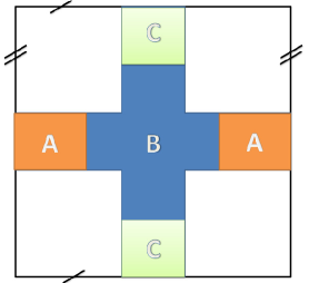
Figure 1: A torus (the top and bottom sides and left and right sides are identified). Subregions $A,\,B,\,C$ are defined as shown. Regions $A$ and $C$ are assumed to be well separated as compared to the correlation length. The regions $AB$ and $BC$ correspond to bipartitions of the torus into cylinders in orthogonal directions.

In order to isolate the topological part of the entropy, we assume that the regions $A$ and $C$ are well separated compared to the correlation length of the gapped ground state. Then, the local contributions cancel in the combination above: $S^{\rm local}_{ABC}+S^{\rm local}_{B}-S^{\rm local}_{AB}-S^{\rm local}_{BC}\rightarrow 0$. This can be argued following Refs.levin2006 ; kitaev2006 . For example, consider a local deformation near region $A$’s boundary far away from the other regions. This change will be in $S^{\rm local}_{ABC}$, but a nearly identical contribution will also appear in $S^{\rm local}_{AB}$, since it only differs by the addition of a distant region. These will cancel in the combination above. Thus, we can rewrite the Eqn. 3 as:

$$S^{\rm topo}_{ABC}+S^{\rm topo}_{B}-S^{\rm topo}_{AB}-S^{\rm topo}_{BC}\leq 0$$ (4)

This inequality implies the TEEs expected from the disc is not legal for the torus.

For regions where the boundary is topologically trivial and contractible (such as $ABC$ or $B$), one expects the TEE to be independent of the surface on which they are defined, and hence $S^{\rm topo}_{ABC}=S^{\rm topo}_{B}=-\gamma$. Only regions $AB$ and $BC$, whose boundaries wrap around the torus, are sensitive to the topology of the space they are defined on. Their TEEs satisfy:

$$\gamma_{BC}+\gamma_{AB}\leq 2\gamma$$ (5)

where we have defined $S^{\rm topo}_{AB(BC)}=-\gamma_{AB(BC)}$. Clearly this does not allow both the TEEs to to be $2\gamma$. In fact if one of them attains its maximal disc value, the other must vanish. Note, the TEE reduces the total entropy. Thus, when the entropy of a cut along one of the cycles of the torus attains its minimum value, i.e. we have most knowledge about the state on the cut, then along the orthogonal direction, the entropy associated with a cut must attain its maximal value, implying our knowledge is the least. Therefore this can be thought of as an uncertainty relation, between cuts that wrap around different directions of the torus.

II.2 Ground State Dependence of TEE in a Chiral Spin Liquid

In this subsection, to illustrate the state dependence of TEE, we study the entanglement properties in a lattice model of an $SU(2)$ spin-symmetric CSL on a torus. The CSL has the same topological order as the half filled Landau level $\nu=1/2$ Laughlin state kalmeyer ; thomale of bosons (these bosons can be thought of as residing at the location of spin up moments), and has two-fold degenerate ground states on the torus. The topological order in CSL can be confirmed by calculating its topological entanglement entropy (TEE) numerically using Monte Carlo and verifying that it is non-zero and agrees with the field theoretical predictions frank2011 . We note that here we are working with a generic wave function in this phase defined on a lattice, rather than with idealized zero correlation length states or the topological field theory. This will introduce new conceptual issues - in particular, the connection between MESs and lattice ground states will be discussed.

We begin by reporting the results of a numerical experiment. We extract TEE of linear combinations of the two ground states of the CSL, and show that it indeed depends systematically on the chosen linear combination, when the entanglement cut wraps around the torus. We will then predict theoretically the dependence and find excellent agreement as shown in Fig. 3.

II.2.1 Numerical Study of Ground State Dependence of TEE in Gutzwiller Projected CSL states

Wave functions of an SU(2) spin symmetric CSL are obtained in the slave particle construction. We write the spins as bilinear in fermions $\vec{S}=\frac{1}{2}f^{\dagger}_{\sigma}[\vec{\sigma}]_{\sigma\sigma^{\prime}}f_{\sigma^{\prime}}$ and assume a chiral d-wave state for the fermions. Operationally, the spin wavefunctions are obtained by Gutzwiller projection of a $d_{x^{2}-y^{2}}+id_{xy}$ superconductor to one fermion per site. More technical details regarding this wave function are in Appendix B. We consider the system on a torus. Before projection, one can write down different fermion states, by choosing periodic or anti-periodic boundary conditions along $\hat{x}$ and $\hat{y}$ directions. These boundary conditions are invisible to the spin degrees of freedom which are bilinear in the fermions and lead to degenerate ground statesRead89 . We denote the ground states by the mean field fluxes in $\hat{x}$ and $\hat{y}$ directions as $\left|\varphi_{1},\varphi_{2}\right\rangle$, $\varphi_{1,2}=0,\pi$. The two fold degeneracy of the CSL implies that only two of the four ground states $\left|0,0\right\rangle$, $\left|\pi,0\right\rangle$, $\left|0,\pi\right\rangle$, $\left|\pi,\pi\right\rangle$ are linearly independent. Here we consider linear combinations of $\left|0,\pi\right\rangle$ and $\left|\pi,0\right\rangle$, which we have numerically checked to be indeed orthogonal for the system sizes that we consider:

$$\left|\Phi(\phi)\right\rangle=\cos\phi\left|0,\pi\right\rangle+\sin\phi\left|\pi,0\right\rangle$$ (6)

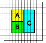
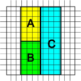
Figure 2: The separation of the system into subsystem $A$, $B$, $C$ and environment, periodic or antiperiodic boundary condition is employed in both $\hat{x}$ and $\hat{y}$ directions. a: The subsystem $ABC$ is an isolated square and the measured TEE has no ground state dependence. b: The subsystem $ABC$ takes a non-trivial cylindrical geometry and wraps around the $\hat{y}$ direction, and TEE may possess ground stated dependence.

We calculated TEE for the state $|\Phi\rangle$ using VMC method and Gutzwiller projected wave functions based on Eqn.32. An efficient VMC algorithm which allows to study a linear combination of Gutzwiller projected wave functions was developed and detailed in Appendix A. To our knowledge, this is the first numerical study to accomplish this.

The geometry and partition of the system are shown in Fig. 2b. The total system size is 12 lattice spacings in both directions with rectangles $A$ and $B$ being $6\times 4$ and rectangle $C$ $12\times 4$. Note that the subsystems $AC$, $BC$, $AB$, $C$ and $ABC$ all wrap around $\hat{y}$ direction so that their TEE will all be equal (and denoted $\gamma^{\prime}$). This is the quantity we wish to access. For contractible subsystems $A$ and $B$ it remains the same as that expected for a region with a single boundary, cut out of a topologically trivial surface (such as a bigger disc) $\gamma$. We use the construction due to Kitaev and Preskill kitaev2006 and effectively isolate the topological contributions in the limit of small correlation length, by evaluating the combination of entropies $S_{A}+S_{B}+S_{C}-S_{AB}-S_{AC}-S_{BC}+S_{ABC}$. This combination is related to the TEE by:

$$-2\gamma+\gamma^{\prime} = S_{A}+S_{B}+S_{C}$$ (7)

$$- S_{AB}-S_{AC}-S_{BC}+S_{ABC}$$

$$= 2S_{A}-2S_{AC}+S_{ABC}$$

In the second line we have exploited symmetries of the construction to reduce the problem to calculation of the Renyi entropy $S_{2}$ of three regions $A$, $AC$ and $ABC$ for each $\phi$. To measure $S_{2}$ numerically, we calculated the expectation value of a $\rm{Swap_{A}}$ operator, see Reffrank2011 for an elaboration of the method used. Our results for $2\gamma-\gamma^{\prime}\left(\phi\right)$ corresponding to different linear combinations parameterized by $\phi$ are shown in Fig.3. This is one of the main results of this work.

We note the TEE strongly depends on the particular linear combination chosen. The zero of the curve implies that the TEE $\gamma^{\prime}=2\gamma$, intuitive value for an entanglement cut with two boundaries. The corresponding state is the MES. We note that the MES occurs at a nontrivial angle. Understanding this requires connecting the lattice states and the field theory which is done below. We predict this angle to be $0.125\pi$ and the overall TEE dependence to be Eqn. 13, which is plotted as the solid curve Fig. 3, in rather good agreement with the numerical data.

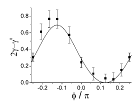
Figure 3: Numerically measured TEE $2\gamma-\gamma^{\prime}$ for a CSL ground state from linear combination $\left|\Phi\right\rangle=\cos\phi\left|0,\pi\right\rangle+\sin\phi\left|\pi,0\right\rangle$ as a function of $\phi$ with VMC simulations using geometry in Fig. 2b. The solid curve is the theoretical value from Eqn. 13. The periodicity is $\pi/2$.

II.2.2 Theoretical Evaluation of Ground State Dependence of TEE in CSL wavefunctions

A calculation of ground-state dependence of TEE involves two steps. In the first step, we ask the following question: given a state expressed as a linear combination of MESs, what is the expected TEE? For the CSL, this question has already been answered by Ref. dong2008, that TEE for a state $|\psi\rangle=a_{1}|1\rangle+a_{2}|2\rangle$ is

$$\gamma^{\prime}-2\gamma=\log\left(|a_{1}|^{4}+|a_{2}|^{4}\right)$$ (8)

where $|1\rangle,\,|2\rangle$ are MESs for cutting the torus in the direction in question.

Second, we need to understand the relation between the MES and the physical states that appear in the Gutzwiller wave function. In general it appears that the only way to identify MESs in a generic wave function is by calculating the TEE. However, when the lattice model has additional symmetry, that can also be used to identify MESs. Here, we have a $12\times 12$ system defined on a square lattice and we will exploit the $\pi/2$ rotation symmetry to establish a connection between the flux states $|\varphi_{1},\,\varphi_{2}\rangle$ of the Gutzwiller ansatz and the MESs.

The Gutzwiller projected ground states of the CSL, $\left|0,0\right\rangle$ and $\left|\pi,\pi\right\rangle$ are clearly invariant under a $\pi/2$ rotation symmetry upto a phase factor. A simple calculation shows that the $\left|0,0\right\rangle$ state acquires phase factor $-1$ while the $\left|\pi,\pi\right\rangle$ state acquires no phase under rotation. Similarly, the states $\frac{1}{\sqrt{2}}\left(\left|0,\pi\right\rangle\pm\left|\pi,0\right\rangle\right)$ acquire a phase $\pm 1$ under rotation. Having established the transformation of lattice states under rotation, we now study how the MESs in the field theory respond to rotations. We will see that $\pi/2$ rotation in the basis of the MESs is described by the modular $\mathcal{S}$ matrix. The eigenvectors of the modular $\mathcal{S}$ matrix will then be identified with lattice states that are rotation eigenstates.

The CSL has the same topological order as the half filled Landau level $\nu=1/2$ Laughlin state kalmeyer ; thomale of bosons. The field theory describing the topological order of a $\nu=1/k$ Laughlin state is described by the following Chern-Simons action. Note, here only the very long wavelength degrees of freedom are retained:

$$S=\int\frac{k}{4\pi}a_{\mu}\partial_{\upsilon}a_{\lambda}\epsilon^{\mu\upsilon\lambda}$$

One can define the Wilson loop operators $T_{1}=e^{i\theta_{1}}=e^{i\oint a_{x}dx}$ and $T_{2}=e^{i\theta_{2}}=e^{i\oint a_{y}dy}$ around the two distinct cycles of the torus. In terms of $\theta_{i}$, the action is given by

$$S=i\frac{k}{2\pi}\int dt\theta_{1}\dot{\theta_{2}}$$

which implies that at the operator level $\left[\theta_{1},\theta_{2}\right]=i\frac{2\pi}{k}$ or

$$T_{1}T_{2}=T_{2}T_{1}e^{2\pi i/k}$$

Owing to the above relation, there are $k$ orthogonal ground states $|\psi_{m}\rangle$ that can be chosen to transform under $T_{i}$ as

$$T_{2}|\psi_{m}\rangle = e^{2\pi i(m-1)/k}|\psi_{m}\rangle$$

$$T_{1}|\psi_{m}\rangle = |\psi_{m+1}\rangle$$

In the case of a CSL phase, $k=2$. Let us label the two degenerate ground states as $\left(1,0\right)^{T}$ and $\left(0,1\right)^{T}$, which are eigenstates of $T_{2}$:

$$T_{2}\left(1,0\right)^{T} = \left(1,0\right)^{T}$$

$$T_{2}\left(0,1\right)^{T} = -\left(0,1\right)^{T}$$

$$T_{1}\left(1,0\right)^{T} = \left(0,1\right)^{T}$$

$$T_{1}\left(0,1\right)^{T} = \left(1,0\right)^{T}$$

The last two equations are due to the commutation relation $T_{1}T_{2}=-T_{2}T_{1}$. It follows that the eigenstates of $T_{1}$ are $\left(1,1\right)^{T}/\sqrt{2}$ and $\left(1,-1\right)^{T}/\sqrt{2}$.

The significance of the $T_{1,2}$ eigenstates is that they are MESsdong2008 , for cuts whose boundaries are parallel to the loops used to define $T_{1,2}$. This is because eigenstates of these loop operators have a fixed value of flux enclosed within the relevant cycle of the torus, which minimizes the entanglement entropy for a parallel cut as shown in Fig. 4.

Now consider a $\pi/2$ rotation, under which $\theta_{1}\rightarrow\theta_{2}$ and $\theta_{2}\rightarrow-\theta_{1}$ so $T_{1}\rightarrow T_{2}$ and $T_{2}\rightarrow T_{1}^{-1}=T_{1}$. Thus, the matrix representing the effect of $\pi/2$ rotation for CSL in $T_{2}$ eigenstate basis is:

$$\mathcal{S}=\left(\begin{array}[]{cc}\frac{1}{\sqrt{2}}&\frac{1}{\sqrt{2}}\\ \frac{1}{\sqrt{2}}&-\frac{1}{\sqrt{2}}\end{array}\right)$$ (11)

Note that we have used the symbol $\mathcal{S}$ for the above matrix because it is indeed the modular $\mathcal{S}$ matrix of the Chern-Simons topological quantum field theory corresponding to a CSL. We recall that the modular $\mathcal{S}$ matrix transforms the eigenstates of one Wilson loop operator $T_{2}$ to those of $T_{1}$. We will return to the discussion of deriving $\mathcal{S}$ matrix for CSL state using the entanglement properties of the ground states in Sec. III.1. Here we restrict ourselves to the calculation of TEE for the CSL.

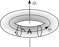
Figure 4: The presence of two fluxes $\theta_{1}$ and $\theta_{2}$ on a torus. In cylindrical cut $A$ that wraps around $\hat{y}$ direction, only $\theta_{2}$ is a measurable.

Since we are interested in the entanglement entropy with respect to the cut shown in Fig. 4, let us represent all our states in the basis of the eigenstates of $T_{2}$, i.e. the states $(0,1)$ and $(1,0)$. Then, by matching eigenstates of the $\mathcal{S}$ matrix in the above basis and rotation eigenstates of the lattice problem, we conclude:

$$\left|\pi,0\right\rangle = \left(\sin\frac{\pi}{8},\cos\frac{\pi}{8}\right)^{T}$$

$$\left|0,\pi\right\rangle = \left(\cos\frac{\pi}{8},-\sin\frac{\pi}{8}\right)^{T}$$

We can now expand the general linear combination state $|\Phi(\phi)\rangle$ in MESs:

$$\left|\Phi\right\rangle = \cos\phi\left|0,\pi\right\rangle+\sin\phi\left|\pi,0\right\rangle$$ (12)

$$= \left(\cos\left(\phi-\frac{\pi}{8}\right),\sin\left(\phi-\frac{\pi}{8}\right)\right)$$

Then, according to Eqn. (2), theoretically one expects the following expression for TEE:

$$2\gamma-\gamma^{\prime} = \log\frac{4}{3+\sin\left(4\phi\right)}$$ (13)

which is compared with the numerical data in Fig. 3. The MES occur at the value of $\phi=\pi/8$ (mod $\pi/2$).

II.3 Toric code and $Z_{2}$ spin liquid

In this subsection we use the Kitaev’s Toric code model kitaev2003 as a pedagogical example to understand ground-state dependence of TEE and the nature of the MESs for a $Z_{2}$ gauge theory.

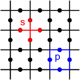
Figure 5: Illustration of a lattice of the toric code model, the links spanned by star and plaquette are highlighted in red and blue, respectively.

Consider the toric code Hamiltonian of spins defined on the links of a square latticekitaev2003 :

$$H=-\sum_{s}A_{s}-\sum_{p}B_{p}$$ (14)

where $s$ and $p$ represent the links spanned by star and plaquette as shown in the Fig.5, and $A_{s}=\prod_{j\in s}\sigma^{x}_{j}$, $B_{p}=\prod_{j\in p}\sigma^{z}_{j}$. Since all individual terms in the Hamiltonian commute with each other, ground states are constructed from the simultaneous eigenstates of all $A_{s}$ and $B_{p}$. Define the operator $W^{z}(C)$ associated with a set of closed curves $C$ on the bonds of the lattice, as follows

$$W^{z}(C) = \prod_{j\in C}\sigma_{j}^{z}$$ (15)

Then the ground state is an equal superposition of all possible loop configurations: $\sum_{C}W^{z}_{ab}(C)|\mbox{vac}_{x}\rangle$, where $|\mbox{vac}_{x}\rangle$ is a state with $\sigma_{x}=-1$ on every site. The closed loops are interpreted as electric field lines of the Z₂ gauge theory. We now consider two geometries, first the cylinder and then the torus. The former case has a pair of degenerate ground states, and is the simplest setting to demonstrate state dependence of TEE.

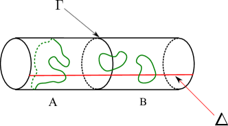
Figure 6: A snapshot of the ground state on the cylinder. Closed-loop strings (“Z₂ electric fields”) can wrap around the cylinder. The ground states are doubly degenerate, corresponding to even and odd winding number sectors. The total number of string crossings the cut $\Delta$ equals the winding number, modulo $2$. The number of string crossings at the boundary $\Gamma$ is even in the degenerate ground states.

II.3.1 Cylinder Geometry

On a cylinder, the Hamiltonian in Eqn.14 leads to a pair of degenerate ground states (the $A_{s}$ part of the Hamiltonian is suitably modified at the boundary of the cylinder to only include three links). The two normalized ground states $|\xi_{0}\rangle,|\xi_{1}\rangle$, are given by equal superpositions of electric field loop configurations which have an even and odd winding number around the cylinder respectively (see Fig. 6). Consider now partitioning the cylinder into two cylindrical regions $A$ and $B$. Then the Schmidt decomposition of these ground states can be written as:

$$|\xi_{0}\rangle = \frac{1}{\sqrt{2N_{q}}}\sum_{\{q_{l}\}}\left(|\Psi^{A}_{\{q_{l}\},0}\rangle|\Psi^{B}_{\{q_{l}\},0}\rangle+|\Psi^{A}_{\{q_{l}\},1}\rangle|\Psi^{B}_{\{q_{l}\},1}\rangle\right)$$

$$|\xi_{1}\rangle = \frac{1}{\sqrt{2N_{q}}}\sum_{\{q_{l}\}}\left(|\Psi^{A}_{\{q_{l}\},0}\rangle|\Psi^{B}_{\{q_{l}\},1}\rangle+|\Psi^{A}_{\{q_{l}\},1}\rangle|\Psi^{B}_{\{q_{l}\},0}\rangle\right)$$

where the $N_{q}$ distinct configurations represented by $\{q_{l}\}$ denotes the electric field configurations at the cut. The number of field lines crossing the cut is always even, since the ground state is composed of closed loops. For trivial bipartitions, this exhausts all terms in the Schmidt decomposition levin2006 . However, given that the boundary of the cut is non-contractible, the additional index $0,\,1$ appears which counts the parity of electric field winding around the cylinder, within a partition. These are correlated between the two partitions, for the fixed winding number ground states. This is the key difference from a trivial bipartition, leading to the ground-state dependence of TEE.

We now calculate the entanglement entropy associated with such a cut for an arbitrary linear combination of these two ground states $|\Psi\rangle=c_{0}|\xi_{0}\rangle+c_{1}|\xi_{1}\rangle$, with unit norm. Using Eqn. LABEL:eq:decomp one can easily verify:

$$|\Psi\rangle=\frac{1}{\sqrt{2N_{q}}}\sum_{\{q_{l}\}} [(c_{0}+c_{1})|\Psi^{A}_{\{q_{l}\},+}\rangle|\Psi^{B}_{\{q_{l}\},+}\rangle$$

$$+ (c_{0}-c_{1})|\Psi^{A}_{\{q_{l}\},-}\rangle|\Psi^{B}_{\{q_{l}\},-}\rangle]$$ (17)

where $|\Psi^{A(B)}_{\{q_{l}\},\pm}\rangle=\left(|\Psi^{A(B)}_{\{q_{l}\},0}\rangle\pm|\Psi^{A(B)}_{\{q_{l}\},1}\rangle\right)/\sqrt{2}$. For a Schmidt decomposition $|\Psi\rangle=\sum_{a}\sqrt{\lambda_{a}}|\Psi^{A}_{a}\rangle|\Psi^{B}_{a}\rangle$ the $n$th Renyi entropy is given by: $S_{n}=\frac{1}{1-n}\log\left(\sum_{a}\lambda_{a}^{n}\right)$. We arrive at: $S_{n}=\frac{1}{1-n}\log N_{q}^{1-n}[p_{+}^{n}+p_{-}^{n}]$, where $p_{\pm}=|c_{0}\pm c_{1}|^{2}/2$. Recognizing that the closed loop constraint leads to $N_{q}=2^{L-1}$, where $L$ is the length of the cut, and using the definition of TEE in Eqn. 1 we have:

$$\gamma^{\prime}_{n}=\log 2-\frac{1}{1-n}\log(p_{+}^{n}+p_{-}^{n})$$ (18)

Thus, for the electric field winding eigenstates $|\xi_{0,1}\rangle$ where $p_{\pm}=1/2$, the TEE vanishes. However, for their equal superpositions when one of $p_{+}$ or $p_{-}$ vanishes, the TEE attains its maximal value $\log 2$. These are eigenstates of the Wilson loop operator that encircles the cylinder and measures the Z₂ magnetic flux (vison number) threading it. An example of such a flux operator is $F=\prod_{j\in Q}\sigma_{j}^{z}$, where $Q$ is a closed curve that loops once around the cylinder, such as the boundary $\Gamma$ in Fig. 6. Since TEE reduces the entanglement entropy, the maximum TEE states correspond to MESs. Why these MESs are eigenstates of flux through the cylinder for this particular cut? The number of electric field lines crossing the boundary $\Gamma$ is always even. This constraint carries some information and hence lowers the entropy by bringing in the standard TEE of $\log{2}$. On the other hand, the topology of the cut boundary $\Gamma$ allows for a determination of which magnetic flux sector the cylinder is in. A state that is not an eigenstate of magnetic flux through the cylinder leads to a loss of information and hence a positive contribution to the total entanglement entropy (and reduces TEE). This suggests that the MESs are eigenstates of loop operators which can be defined parallel to the cut $\Gamma$. This is further substantiated by the result for the torus case discussed below, where they are simultaneous eigenstates of magnetic flux enclosed by the cut and electric flux penetrating the cut.

II.3.2 Torus Geometry

The four degenerate ground states are distinguished by the even-odd parity of the winding number of electric field lines around the two cycles of the torus. The operator $W^{z}(C)$, which generates the set of closed loops $C$ can be used to write the ground states:

$$|\xi_{ab}\rangle=\sum_{C}W^{z}_{ab}(C)|\mbox{vac}_{x}\rangle$$

where the subscript $a$ ($b$) takes on binary values $0,1$ and denotes whether the loops $C$ belong to the even or odd winding number sectors along the $\hat{x}$ ($\hat{y}$) direction, and $|\mbox{vac}_{x}\rangle$ is a state with $\sigma_{x}=-1$ on every site. The four ground states cannot be mixed by any local operator and hence realize a $Z_{2}$ topological order. Let us consider a ground state as the following linear combination:

$$\left|\Psi\right\rangle=\sum_{a,b=0,1}c_{a,b}\left|\xi_{ab}\right\rangle$$ (19)

We are interested in calculating entanglement entropy for the state $\left|\Psi\right\rangle$ corresponding to the partition shown in the Fig.4 and the dependence of TEE on parameters $c_{a,b}$. After straightforward algebra (see details in Appendix C), one finds the following expression for subsystem A with boundaries of length $L$:

$$S_{n}=L\textrm{log}(2)-\gamma^{\prime}_{n}$$

where

$$\gamma^{\prime}_{n}=2\,\textrm{log}\,\left(2\right)-\frac{1}{1-n}\log\sum_{j=1}^{4}p_{j}^{n}$$ (20)

and

$$p_{1} = \frac{|c_{00}+c_{01}|^{2}}{2}$$

$$p_{2} = \frac{|c_{00}-c_{01}|^{2}}{2}$$

$$p_{3} = \frac{|c_{10}+c_{11}|^{2}}{2}$$

$$p_{4} = \frac{|c_{10}-c_{11}|^{2}}{2}$$ (21)

This is indeed consistent with Eqn.2, given that $\gamma=\log D=\log 2$ and $d_{j}=1$ for an Abelian topological order with $D^{2}=4$ degenerate ground states. Further, Eqn.20 readily leads to the following four MESs:

$$|\Xi_{1}\rangle=\frac{1}{\sqrt{2}}(|\xi_{00}\rangle+|\xi_{01}\rangle)$$

$$|\Xi_{2}\rangle=\frac{1}{\sqrt{2}}(|\xi_{00}\rangle-|\xi_{01}\rangle)$$

$$|\Xi_{3}\rangle=\frac{1}{\sqrt{2}}(|\xi_{10}\rangle+|\xi_{11}\rangle)$$

$$|\Xi_{4}\rangle=\frac{1}{\sqrt{2}}(|\xi_{10}\rangle-|\xi_{11}\rangle)$$ (22)

What is the physical significance of these four states being the MESs? Similar to the cylinder geometry case, these states are the simultaneous eigenstates of Wilson loop operators that encircles the torus and measures the $Z_{2}$ magnetic and electric fluxes threading it, as shown in Table 1 and Fig. We leave more detailed algebra to Appendix C.

When $\gamma^{\prime}_{n}$ is maximized, the corresponding $S_{n}$ is minimized, providing the maximum possible information about a given state. Since the cut is made along $\hat{y}$, it can measure the $Z_{2}$ magnetic and electric fluxes directed parallel to $\hat{x}$. Hence the MES $|\Xi_{\alpha}\rangle$ with definite magnetic and electric flux sectors, maximizes the TEE with $\gamma_{topo}=2\log(2)$, a contribution of $\log(2)$ from each of the two boundaries. As one linear superposes different MESs $|\Xi_{\alpha}\rangle$, the information obtained from measuring magnetic and electric sectors becomes scrambled; especially, at the extreme case of equal superposition of $|\Xi_{\alpha}\rangle$, all information about the global quantum numbers has been lost and we have $\gamma^{\prime}=0$. This offers another example where MESs are the eigenstates of loop operators defined on the cylinder from the entanglement cut.

MES	$T_{y}$	$F_{y}$	quasi-particle
$\Xi_{1}$	0	0	$1$
$\Xi_{2}$	1	0	$m$
$\Xi_{3}$	0	1	$e$
$\Xi_{4}$	1	1	$em$

Table 1: List of $Z_{2}$ magnetic flux $T_{y}$, $Z_{2}$ electric flux $F_{y}$ and corresponding quasi-particle of Wilson loop operator for the four MESs $|\Xi_{\alpha}\rangle$ of the toric code with system geometry in Fig.4. The definitions of $T_{y}$ and $F_{y}$ are in Appendix C.

Numerical Verification in a Generic Z₂ wavefunction: To provide an example of the state dependence of TEE in a $Z_{2}$ topologically ordered beyond the simple toric code model, we employ our VMC method to calculate the TEE of an $SU(2)$ symmetric $Z_{2}$ spin liquid for a cylindrical bipartition of the torus. This is a generic spin wave function, and has a finite correlation length unlike the toric code. It is obtained by Gutzwiller projecting a mean-field BCS state on a square lattice (see Appendix B for details).

For the $Z_{2}$ spin liquid wave function obtained by Gutzwiller projecting the above mean-field ground state, a calculation of TEE corresponding to a disc shaped region $A$ was performed in Ref.frank2011 . It was established that the state is indeed topologically ordered with the value of $\gamma\approx 0.584\pm 0.089$, close to the expected theoretical value of $\gamma=\log 2\approx 0.693$. Here we are concerned with the calculation of TEE for a cylindrical bipartition. We study systems with 12 lattice spacings in the $\hat{x}$ direction and 8 lattice spacings in the $\hat{y}$ direction. The subsystem separation scheme is similar to Fig.2b, where $A$ and $B$ are $4\times 4$ squares and $C$ is a $4\times 8$ rectangle, see Fig. 7. The TEE $2\gamma-\gamma^{\prime}$ can be evaluated in a similar way as Eqn.7.

By employing periodic boundary conditions in both directions, the state we study has zero magnetic flux along both directions, but it is not a MES. Instead, it is an equal superposition of two MESs states that have zero magnetic flux and $0$ or $1$ electric flux respectively through the cylinder. Therefore, according to Eqn.20, with $p_{1}=p_{3}=1/2,p_{2}=p_{4}=0$ and Renyi index $n=2$, one finds:

$$\gamma^{\prime} = 2\log(2)+\log(\sum_{j=1}^{4}p_{j}^{2})=\log\left(2\right)$$

$$2\gamma-\gamma^{\prime} = \log\left(2\right)$$

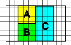
Figure 7: The separation of the system into subsystem $A$, $B$, $C$ and environment, periodic boundary condition is employed in both $\hat{x}$ and $\hat{y}$ directions. The subsystem $ABC$ takes a non-trivial cylindrical geometry and wraps around the $\hat{y}$ direction.

The VMC simulation yields $2\gamma-\gamma^{\prime}=0.576\pm 0.108$, close to the expected theoretical value $\log(2)\sim 0.693$. The smaller than expected values for both $\gamma$frank2011 ; isakov2011 and $\gamma^{\prime}$ are probably due to quasi-particle excitations across a finite gap, causing breaking of $Z_{2}$ electric field lines over the finite system size we consider. Indeed, spin correlations decay slower for the $Z_{2}$ state, as compared to the CSL, which also arrives closer to its expected value of TEE for both cylindrical bipartition as well as for the disc shaped region $A$ frank2011 .

III Extracting Statistics from Topological Entanglement Entropy

The modular $\mathcal{S}$ and $\mathcal{U}$ matrices describe the action of certain modular transformations on the degenerate ground states of the topological quantum field theory. On the other hand, the braiding and statistics of quasi-particles are encoded in the $\mathcal{S}$ and $\mathcal{U}$ matrices. For Abelian phases, the $ij$’th entry of the $\mathcal{S}$ matrix corresponds to the phase the $i$’th quasi-particle acquires when it encircles the $j$’th quasi-particle. The $\mathcal{U}$ matrix is diagonal and the $ii$’th entry corresponds to the phase the $i$’th quasi-particle acquires when it is exchanged with an identical one. Since the MESs are the eigenstates of the nonlocal operators defined on the entanglement cut, the MESs are the canonical basis for defining $\mathcal{S}$ and $\mathcal{U}$. The modular matrices are just certain unitary transformations of the MES basis. As argued in Appendix D, the $\mathcal{S}$ matrix acts on MESs as an operator that implements $\pi/2$ rotation while the $\mathcal{U}S$ matrix corresponds to $2\pi/3$ rotation of MESs.

III.1 Modular S-matrix of CSL from TEE

Let’s consider the CSL wave functions studied in Sec. II.2.1, and assume that we did not have any information about the individual quantum dimensions or the modular $\mathcal{S}$ matrix. The only information that is provided is the two-fold degenerate ground-state wave functions $|\pi,0\rangle$ and $|0,\pi\rangle$. We construct the linear combination $|\Phi\rangle$ as Eqn.12 and calculate its TEE for a non-trivial bipartition as Fig.4 on a $\pi/2$ rotation symmetric lattice. Consequently, we get the $2\gamma-\gamma^{\prime}$ dependence on parameter $\phi$ in Fig.3.

We notice that the minimum of the $2\gamma^{\prime}-\gamma$ attained is approximately zero. According to Eqn.2, this implies that at least one of the quantum dimensions $d_{i}$ should be $1$. Since the total quantum dimension $D=\sqrt{d_{0}^{2}+d_{1/2}^{2}}=\sqrt{2}$, this implies that $d_{0}=d_{1/2}=1$. Also, we see that the MES lies at $\phi\approx 0.14\pi$ by fitting Fig.3 to Eqn.2.

For system with square geometry the $\mathcal{S}$ matrix describes the action of $\pi/2$ rotation on the MESs. Since the two states $|0,\pi\rangle$ and $|\pi,0\rangle$ transform into each other under $\pi/2$ rotation, this implies that in the basis $\{|0,\pi\rangle,|\pi,0\rangle\}$, the modular $\mathcal{S}$ matrix is given by the Pauli matrix $\sigma_{x}$. To change the basis to MESs, we just need a unitary transformation $V$ that rotates $|0,\pi\rangle\,|\pi,0\rangle$ basis to the MESs basis. The $V$ is determined by the fact that one needs to rotate $|0,\pi\rangle\,|\pi,0\rangle$ basis by an angle $\approx 0.14\pi$ to obtain MES (this is the numerically determined value, the exact value being $\pi/8$). Therefore,

$$\mathcal{S}=V^{\dagger}\left(\begin{array}[]{cc}0&1\\ 1&0\end{array}\right)V$$

where

$$V\approx\left(\begin{array}[]{cc}\cos(0.14\pi)&-\sin(0.14\pi)e^{i\varphi}\\ \sin(0.14\pi)&\cos(0.14\pi)e^{i\varphi}\end{array}\right)$$

from the two MESs: $(\cos(0.14\pi),\sin(0.14\pi))^{T}$ and $(-\sin(0.14\pi),\cos(0.14\pi))^{T}$ and $\varphi$ is an undecided phase. This yields the following value for the approximate modular $\mathcal{S}$ matrix

$$\mathcal{S}\approx\left(\begin{array}[]{cc}\sin(0.28\pi)&\cos(0.28\pi)e^{i\varphi}\\ \cos(0.28\pi)e^{-i\varphi}&-\sin(0.28\pi)\end{array}\right)$$

The existence of an identity particle requires positive real entries in the first row and column and implies $\varphi=0$, which gives:

$$\mathcal{S}\approx\left(\begin{array}[]{cc}0.77&0.63\\ 0.63&-0.77\end{array}\right)$$

Comparing this result with the exact expression in Eqn. 11, we observe that even though the $\mathcal{S}$ matrix obtained using our method is approximate, some of the more important statistics can be extracted rather exactly. The above $\mathcal{S}$ matrix tells us that the quasi-particle corresponding to $d_{0}=1$ does not acquire any phase when it goes around any other particle and corresponds to an identity particle as expected, while the quasi-particle corresponding to $d_{1/2}=1$ has semion statistics since it acquires a phase of $\pi$ when it encircles another identical particle. Numerical improvements can further reduce the error in pinpointing the MES and thereby leading to a more accurate value of the $\mathcal{S}$ matrix. As another application, we study the action of modular transformation on the MESs $|\Xi_{\alpha}\rangle$ for the $Z_{2}$ gauge theory in Appendix E.

III.2 Algorithm for extracting modular $\mathcal{S}$ matrix from TEE

In the last subsection and Appendix E we calculated the modular $\mathcal{S}$ matrices for the CSL and $Z_{2}$ toric code model respectively using the transformation properties of the basis states $|\xi_{ab}\rangle$ under $\pi/2$ rotation transformations $\mathcal{R}$ and translating it into the canonical basis of MESs $|\Xi_{i}\rangle$: $\mathcal{S}=U^{\dagger}\mathcal{R}U$. However, such $\pi/2$ rotation symmetry is not necessary. Even without symmetry, it is possible to obtain the $\mathcal{S}$ matrix by studying the modular transformation between certain nontrivial pair of sets of MESs.

Starting from the definition, the modular $\mathcal{S}$ matrix has the following expression:

$$\mathcal{S}_{\alpha\beta}=\frac{1}{D}\left\langle\Xi_{\alpha}^{\hat{x}}|\Xi_{\beta}^{\hat{y}}\right\rangle$$ (27)

Here $D$ is the total quantum dimension and $\hat{x}$ and $\hat{y}$ are two directions on a torus. Eqn.27 is just a unitary transformation between the particle states along different directions. In the case of a square system as in the last subsection, the $\mathcal{S}$ matrix acts as a $\pi/2$ rotation on the MES basis $\left|\Xi_{\beta}^{\hat{y}}\right\rangle$. In general, however, $\hat{x}$ and $\hat{y}$ do not need to be geometrically orthogonal, and the system does not need to be rotationally symmetric, as long as the loops defining $\left|\Xi_{\alpha}^{\hat{x}}\right\rangle$ and $\left|\Xi_{\beta}^{\hat{y}}\right\rangle$ interwind with each other. Therefore, the modular $\mathcal{S}$ matrix can be derived even without any presumed symmetry of the given wave functions. Note that there is an undetermined phase for each $\left|\Xi_{\alpha}^{\hat{x}}\right\rangle$ and $\left|\Xi_{\beta}^{\hat{y}}\right\rangle$, therefore a phase freedom between the rows (columns), which may be fixed by the existence of an identity particle.

Let’s start with the two primitive vectors $w_{1}$ and $w_{2}$ and determine the transformation of the MESs of $w_{2}$ to those of $w_{2}^{\prime}$ given by:

$$w_{1}^{\prime}=n_{1}w_{1}+m_{1}w_{2}$$

$$w_{2}^{\prime}=n_{2}w_{1}+m_{2}w_{2}$$ (28)

With $n_{1}m_{2}-m_{1}n_{2}=1$ by definition of the modular transformation. We restrict $n_{2}=-1$, which means the cross product:

$$w_{2}\times w_{2}^{\prime}=-w_{2}\times w_{1}=w_{1}\times w_{2}=A$$ (29)

$A$ is the surface area of the torus.

The corresponding modular matrix can be expanded as:

$$\left(\begin{array}[]{cc}n_{1}&1-n_{1}m_{2}\\ -1&m_{2}\end{array}\right) = \left(\begin{array}[]{cc}1&-n_{1}\\ &1\end{array}\right)\left(\begin{array}[]{cc}&1\\ -1\end{array}\right)\left(\begin{array}[]{cc}1&-m_{2}\\ &1\end{array}\right)$$

$$= U^{-n_{1}}SU^{-m_{2}}$$

Correspondingly, according to Appendix D the transformation:

$$\mathcal{R}=\mathcal{U}^{-n_{1}}\mathcal{S}\mathcal{U}^{-m_{2}}$$

Because $\mathcal{U}$ matrix is diagonal by definition, its left (right) matrix products only adds an additional phase factor to each row (column) and can be eliminated. Therefore, without any argument on the symmetry, the generalized algorithm:

1. Given a set of ground state wave functions $\left|\xi_{\alpha}\right\rangle$, calculate the TEE of an entanglement bipartition along $w_{2}$ direction, for a linear combination $\left|\Phi\right\rangle=\sum c_{\alpha}\left|\xi_{\alpha}\right\rangle$ . Search for the minimum of TEE $2\gamma-\gamma^{\prime}$ in the $c_{\alpha}$ parameter space. That gives one MES $\left|\Xi_{\beta}\right\rangle$ and the corresponding quantum dimension $2\log\left(d_{\beta}\right)=2\gamma-\gamma^{\prime}$. Note that the existence of an identity particle ensures at least one minimum TEE $2\gamma-\gamma^{\prime}=0$.

2. iterate step 1 but with $c_{\alpha}$ in the parameter space orthogonal to all previous obtained MESs $\left|\Xi_{\beta}\right\rangle$. Continue this process until we have the expressions for all $\left|\Xi_{\beta}\right\rangle$. This gives a unitary transformation matrix $U_{1}$ with the $\alpha\beta$’th entry being $c_{\alpha\beta}$, which changes the basis from $\left|\xi_{\alpha}\right\rangle$ to $\left|\Xi_{\beta}\right\rangle$. Note that there is a relative $U(1)$ phase degree of freedom for each $|\Xi_{\beta}\rangle$.

3. Repeat step 1 and step 2 but with the entanglement cut along $w_{2}^{\prime}$ direction, which satisfies Eqn. 28 and Eqn. 29, and obtains the unitary transformation matrix $U_{2}$.

4. The modular $\mathcal{S}$ matrix is given by $U_{2}^{-1}U_{1}$ except for an undetermined phase for each MES corresponding to a row or a column. The existence of an identity particle that obtains trivial phase encircling any quasi-particle helps to fix the relative phase between different MESs, requiring the entries of the first row and column to be real and positive. This completely defines the modular $\mathcal{S}$ matrix.

The above algorithm is able to extract the modular transformation matrix $\mathcal{S}$ and hence braiding and mutual statistics of quasi-particle excitations just using the ground-state wave functions as an input. Further, there is no loss of generality for non-Abelian phases, which can be dealt by enforcing the orthogonality condition in step $2$ which guarantees that one obtains states with quantum dimensions $d_{\alpha}$ in an increasing order.

In Appendix E we take the square lattice toric code model as an example once again, but without presuming any symmetry of the system.

III.3 Extracting other modular matrices from TEE

In Appendix E, we calculate the $\mathcal{U}$ matrix for the $Z_{2}$ toric code model, given the simple action of $\mathcal{U}$ on $|\xi_{ab}\rangle$. Though we were unable to find a general algorithm for the $\mathcal{U}$ matrix, as we did for the the $\mathcal{S}$ matrix in the last subsection, in the presence of certain symmetries $\mathcal{U}$ can indeed be extracted given a set of ground-state wave functions $|\xi_{\alpha}\rangle$. This is achieved by first calculating the action $\mathcal{R}$ on the states $|\xi_{\alpha}\rangle$ under this symmetry operation, and then translating it into the action on MESs. Specifically, the corresponding modular matrix is given by $U^{\dagger}\mathcal{R}U$, where the unitary matrix $U$ is obtained through the first two steps of the algorithm in the last subsection.

The aforementioned symmetry to extract $\mathcal{S}$ matrix is the $\pi/2$ rotation, as shown in Sec. III.1 and the first example in Appendix E, but it may be generalized to symmetries such as rotation of other angles and even reflection symmetry (see Appendix D). More interestingly, when the symmetry operation $\mathcal{R}$ is a $2\pi/3$ rotation, one gets the $\mathcal{U}S$ matrix. Hence, if one starts with an arbitrary basis $|\xi_{\alpha}\rangle$ for the degenerate ground state manifold of a topological order, the problem of $\mathcal{S}$ and $\mathcal{U}$ matrices can be reduced to the transformation property of chosen basis states $|\xi_{\alpha}\rangle$ under $\pi/2$ and $2\pi/3$ rotations and the unitary transformation that translates $|\xi_{\alpha}\rangle$ basis to the MESs $|\Xi_{\alpha}\rangle$. To illustrate this point, we extract the $\mathcal{US}$ matrix for the $Z_{2}$ gauge theory in Appendix E by putting the $Z_{2}$ toric code on triangular lattice which has $2\pi/3$ rotation symmetry.

IV Conclusion

In this paper, we studied two topologically ordered phases, the chiral spin liquid (CSL) and the $Z_{2}$ spin liquid using VMC method for Gutzwiller projected wave functions numerically and the $Z_{2}$ toric code model analytically, and showed that the topological entanglement entropy (TEE) depends on the chosen ground state when the entanglement bipartition is topologically nontrivial. We also determined the minimum entropy states (MESs) and explained their physical significance.

As an application of the physical significance of MESs, we suggested an algorithm for extracting the modular transformation matrices that determine the statistics such as quasi-particle self and mutual statistics and individual quantum dimensions. These matrices also determine the central charge of the edge state modulo 8 kitaev_honey . Given the ground states, this algorithm determines the topological order to a large extent. We note that Wen proposed a different way to extract $\mathcal{S}$ and $\mathcal{U}$ matrices by calculating the non-abelian Berry phase wen1990 which in practice may be difficult to implement, especially on a lattice, since it requires calculating the degenerate ground states $\psi_{n}$ of the system as function of the modular parameter $\tau=\omega_{2}/\omega_{1}$ and calculating the derivatives such as $\langle\psi_{n}(\tau)|\partial_{\tau}|\psi_{m}(\tau)\rangle$.

We note that there may be cases where the $\pi/2$ and $2\pi/3$ rotations of the MESs may not be exactly identifiable with the modular $\mathcal{S}$ and $\mathcal{US}$ matrices respectively. This may happen, for example, when the particles have an internal angular momentum which may cause the wavefunction to acquire an additional phase upon rotation, over and above the phase due to underlying topological structure. If the MESs correspond to spin-singlet spin-liquid wave functions (such as CSL studied in this paper) and/or string-net models (such as toric code model) where there is no such internal structure, there should not be such additional phase. Further, since all MESs are locally same, they should all acquire same extra phase due to any local physics and therefore, the extra phase may be separable from the topological phase.

For quantum Hall systems, because of the bulk-edge correspondence, the fusion algebra and topological spin of the bulk quasi-particles also determine the fusion rules and scaling dimensions for the primary fields in the chiral CFT at the edge. Therefore, in the context of quantum Hall systems, the entanglement entropy of the ground state manifold determines robust features of the fields in the corresponding edge CFT.

It would also be interesting to consider generalization of the methods developed in our paper to higher dimensions. Discrete gauge theories furnish the best known theories with long-range entanglement in $D\geq 3$ dimensions and akin to $D=2$, they again support degenerate ground states on the torus. In a recent paper grov2011 , it was shown that these theories again have non-zero TEE that is proportional to $\log(|G|)$, the number of elements in the gauge group. A simple generalization of the method developed in this paper shows that TEE for bipartition that has non-contractible boundaries will again depend on the ground state, and one will again find certain MESs that have the maximum knowledge of the quantum numbers associated with an entanglement cut. Yet we are not aware of simple generalization of modular transformations to higher dimensions, the meaning of the matrix that relates MESs for orthogonal entanglement cuts in higher dimensions requires further investigation.

Acknowledgements: We thank Alexei Kitaev, Michael Levin, Chetan Nayak and Shinsei Ryu for helpful discussions. We acknowledge support from NSF DMR 0645691. A part of this research was performed at Kavli Institute for Theoretical Physics, University of California Santa Barbara, supported by the National Science Foundation under Grant No. NSF PHY05-51164. M. O. was supported in part by Grant-in-Aid for Scientific Research (KAKENHI) No. 20102008.

Appendix A Variational Monte Carlo method for a linear combination of wave-functions

To calculate TEE for wave functions of different linear combinations, it is important to establish a VMC algorithm for wave function as $\left|\Phi\right\rangle=\cos\phi\left|\Phi_{1}\right\rangle+\sin\phi\left|\Phi_{2}\right\rangle$, where we assume $\left|\Phi_{1}\right\rangle$ and $\left|\Phi_{2}\right\rangle$ are properly normalized. In our case, $\left|\Phi_{1}\right\rangle$ and $\left|\Phi_{2}\right\rangle$ are two degenerate ground states, $\left\langle\alpha|\Phi_{1}\right\rangle$ and $\left\langle\alpha|\Phi_{2}\right\rangle$ are single Slater determinants products for each configuration $\left|\alpha\right\rangle$, making $\left\langle\alpha|\Phi\right\rangle$ a sum of two Slater determinants products. However, it may also be generalized to the situation of any wave functions.

In the VMC scenario, the central quantity to evaluate in each Monte Carlo step is the ratio of $\left\langle\alpha^{\prime}|\Phi\right\rangle/\left\langle\alpha|\Phi\right\rangle$, which now has the form:

$$\frac{\left\langle\alpha^{\prime}|\Phi\right\rangle}{\left\langle\alpha|\Phi\right\rangle}=\frac{\cos\phi\left\langle\alpha^{\prime}|\Phi_{1}\right\rangle+\sin\phi\left\langle\alpha^{\prime}|\Phi_{2}\right\rangle}{\cos\phi\left\langle\alpha|\Phi_{1}\right\rangle+\sin\phi\left\langle\alpha|\Phi_{2}\right\rangle}$$ (31)

It is usually much less costly to calculate ratio of $\left\langle\alpha^{\prime}|\Phi_{1}\right\rangle/\left\langle\alpha|\Phi_{1}\right\rangle$ and $\left\langle\alpha^{\prime}|\Phi_{2}\right\rangle/\left\langle\alpha|\Phi_{2}\right\rangle$ if $\left|\alpha\right\rangle$ and $\left|\alpha^{\prime}\right\rangle$ are locally different. For our case, when $\left|\alpha\right\rangle$ and $\left|\alpha^{\prime}\right\rangle$ differ only by one spin(electron) exchange, a much less costly and more accurate algorithm may be implemented for the ratio of determinants with only one different row or column. Unfortunately, after linear superposing different $\left|\Phi_{i}\right\rangle$, Eqn.31 no longer has such a privilege.

However, one can re express Eqn.31 as:

$$\frac{\left\langle\alpha^{\prime}|\Phi\right\rangle}{\left\langle\alpha|\Phi\right\rangle}=\frac{a+bc\cdot\tan\phi}{1+c\cdot\tan\phi}$$

where

$$a = \left\langle\alpha^{\prime}|\Phi_{1}\right\rangle/\left\langle\alpha|\Phi_{1}\right\rangle$$

$$b = \left\langle\alpha^{\prime}|\Phi_{2}\right\rangle/\left\langle\alpha|\Phi_{2}\right\rangle$$

are again ratio of determinants and can be effectively evaluated, and

$$c=\left\langle\alpha|\Phi_{2}\right\rangle/\left\langle\alpha|\Phi_{1}\right\rangle$$

can be efficiently kept track of with $c^{\prime}=a^{-1}bc$ whenever the update $\left|\alpha\right\rangle\rightarrow\left|\alpha^{\prime}\right\rangle$ is accepted in a Monte Carlo step. In practice, numerical check should be included to make sure error for $c$ does not accumulate too much after a certain number of Monte Carlo steps.

This algorithm may be easily generalized to the linear combination of $n$ wave functions, with the computational cost only $n$ times that for a single wave functions.

Appendix B Variational wave functions for Chiral Spin Liquid and Z₂ Spin Liquid.

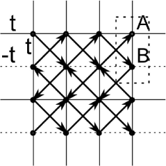
Figure 8: Illustration of a square lattice hopping model connected with a $d+id$ superconductor. While the nearest neighbor hopping is along the square edges with amplitude $t$ ($(-t)$ for hopping along dash lines), the second nearest neighbor hopping is along the square diagonal (arrows in bold), with amplitude $+i\Delta$ ($-i\Delta$) when hopping direction is along (against) the arrow. The two sublattices in the unit cell are marked as A and B.

Chiral Spin Liquid From Gutzwiller Projection: The lattice wave function for the CSL states that we consider are obtained using the slave-particle formalism by Gutzwiller projecting a $d+id$ BCS state kalmeyer ; thomale . Specifically, we Gutzwiller project the ground state of the following Hamiltonian of electrons hopping on a square lattice at half filling:

$$H=\underset{\left\langle ij\right\rangle}{\sum}t_{ij}c_{i}^{\dagger}c_{j}+i\underset{\left\langle\left\langle ik\right\rangle\right\rangle}{\sum}\Delta_{ik}c_{i}^{\dagger}c_{k}$$ (32)

Here $i$ and $j$ are nearest neighbors and the hopping amplitude $t_{ij}$ is $t$ along the $\hat{y}$ direction and alternating between $t$ and $-t$ in the $\hat{x}$ direction from row to row; and $i$ and $k$ are second nearest neighbors connected by hoppings along the square lattice diagonals, with amplitude $i\Delta_{ik}=i\Delta$ along the arrows and $i\Delta_{ik}=-i\Delta$ against the arrows, see Fig.8. The unit cell contains two sublattices A and B. This model leads to a gapped state at half filling and the resulting valence band has unit Chern number. This hopping model is equivalent to a $d+id$ BCS state by an $SU(2)$ Gauge transformation. We take $\Delta=0.5t$ to maximize the relative size of the gap and minimize the finite size effect. Please refer to Reffrank2011 for further details regarding the exact form of the wave function.

Z₂ Spin Liquid from the Gutzwiller Construction:

$$H=-\underset{\left\langle ij\right\rangle}{\sum}\left(\psi_{i}^{\dagger}\mu_{ij}\psi_{j}+h.c.\right)+\underset{i}{\sum}\psi_{i}^{\dagger}a_{0}^{l}\tau^{l}\psi_{i}$$

where $\psi_{i}=\left(f_{\uparrow},f_{\downarrow}^{\dagger}\right)^{T}$. $\tau^{1,2,3}$ are Pauli matrices. The second term is related to chemical potentials, we set $a_{0}^{2,3}=0$, with $a_{0}^{1}$ fixed by the conditions $\left\langle\psi^{\dagger}\tau^{1,2,3}\psi\right\rangle=0$. Matrices $\mu_{ij}$ connecting nearest and next nearest neighbors:

$$\mu_{i,i+x} = \mu_{i,i+y}=-\tau^{3}$$

$$\mu_{i,i+x+y} = \eta\tau^{1}+\lambda\tau^{2}$$

$$\mu_{i,i-x+y} = \eta\tau^{1}-\lambda\tau^{2}$$

This mean field model is readily solvable, with dispersion:

$$E_{k} = \sqrt{\epsilon_{k}^{2}+\left|\Delta_{k}^{2}\right|}$$

$$\epsilon_{k} = 2\left(\cos\left(k_{x}\right)+\cos\left(k_{y}\right)\right)$$

$$\Delta_{k} = 2\eta\left[\cos\left(k_{x}+k_{y}\right)+\cos\left(k_{x}-k_{y}\right)\right]+a_{0}^{1}$$

$$-2i\lambda\left[\cos\left(k_{x}+k_{y}\right)-\cos\left(k_{x}-k_{y}\right)\right]$$

We choose $\eta=\lambda=1.5$ for a large gap and our calculation estimates that the correlation length is as short as $\sim 1.3$ lattice spacings. Please refer to Reffrank2011 for more details on the construction.

Appendix C Minimum entropy states of Toric code model on dividing torus

In this appendix we Schmidt-decompose the individual Toric code ground states $\left|\Psi\right\rangle$ in Eqn.19 for the bipartition of a torus in Fig.4. It is helpful to introduce a virtual cut $\Delta$ which wraps around the torus in the $\hat{x}$ direction, and define $\left|\Psi^{A\left(B\right)}_{{\{q_{l}\}},b}\right\rangle$ as the normalized equal superposition of all the possible configurations of closed-loop strings $C$ in the subsystem $A$ ($B$) with the partition boundary condition specified by ${\{q_{l}=0,1\}}$, $l=1,2,...,L$(so L is the total length of the boundary), and the number of crossings of the virtual cut $\Delta$ modulo 2 equals $b=0,1$. The four ground states may now be expanded as

$$|\xi_{ab}\rangle = \frac{1}{\sqrt{2N_{q}}}\sum_{\{q_{l}\}\in\,a}\left(|\Psi^{A}_{\{q_{l}\},0}\rangle|\Psi^{B}_{\{q_{l}\},b}\rangle\right.$$

$$+\left.|\Psi^{A}_{\{q_{l}\},1}\rangle|\Psi^{B}_{\{q_{l}\},(b+1)\,\textrm{mod}\,2}\rangle\right)$$

Here $\{q_{l}\}\in\,a=0$ $(1)$ denotes that the only even (odd) number of crossings are allowed at the boundary $\Gamma_{1}$ (the number of crossings at the other boundary $\Gamma_{2}$ must be same modulo 2). $N_{q}=2^{L-2}$ equals the total number of valid boundary conditions $\{q_{l}\}\in\,a$ in each parity sector.

We calculate entanglement entropy using the reduced density matrix. Here, $\rho^{A}=\textrm{tr}_{B}|\Psi\rangle\langle\Psi|$ is readily calculated,

$$\rho^{A} = \frac{1}{2N_{q}}\sum_{\{q_{l}\}\in\,\textrm{even}}\left[\left(|c_{00}|^{2}+|c_{01}|^{2}\right)\left(|\Psi^{A}_{\{q_{l}\},0}\rangle\langle\Psi^{A}_{\{q_{l}\},0}|\right.\right.$$

$$+\left.|\Psi^{A}_{\{q_{l}\},1}\rangle\langle\Psi^{A}_{\{q_{l}\},1}|\right)$$

$$\left.+2\,\textrm{Real}(c^{*}_{00}c_{01})\left(|\Psi^{A}_{\{q_{l}\},0}\rangle\langle\Psi^{A}_{\{q_{l}\},1}|+|\Psi^{A}_{\{q_{l}\},1}\rangle\langle\Psi^{A}_{\{q_{l}\},0}|\right)\right]$$

$$+\frac{1}{2N_{q}}\sum_{\{q_{l}\}\in\,\textrm{odd}}\left[\left(|c_{10}|^{2}+|c_{11}|^{2}\right)\left(|\Psi^{A}_{\{q_{l}\},0}\rangle\langle\Psi^{A}_{\{q_{l}\},0}|\right.\right.$$

$$+\left.|\Psi^{A}_{\{q_{l}\},1}\rangle\langle\Psi^{A}_{\{q_{l}\},1}|\right)$$

$$\left.+2\,\textrm{Real}(c^{*}_{10}c_{11})\left(|\Psi^{A}_{\{q_{l}\},0}\rangle\langle\Psi^{A}_{\{q_{l}\},1}|+|\Psi^{A}_{\{q_{l}\},1}\rangle\langle\Psi^{A}_{\{q_{l}\},0}|\right)\right]$$

$$= \frac{1}{2N_{q}}\sum_{\{q_{l}\}\in\,\textrm{even}}\left[|c_{00}+c_{01}|^{2}|\Psi^{A}_{\{q_{l}\},+}\rangle\langle\Psi^{A}_{\{q_{l}\},+}|\right.$$

$$+\left.|c_{00}-c_{01}|^{2}|\Psi^{A}_{\{q_{l}\},-}\rangle\langle\Psi^{A}_{\{q_{l}\},-}|\right]$$

$$+\frac{1}{2N_{q}}\sum_{\{q_{l}\}\in\,\textrm{odd}}\left[|c_{10}+c_{11}|^{2}|\Psi^{A}_{\{q_{l}\},+}\rangle\langle\Psi^{A}_{\{q_{l}\},+}|\right.$$

$$+\left.|c_{10}-c_{11}|^{2}|\Psi^{A}_{\{q_{l}\},-}\rangle\langle\Psi^{A}_{\{q_{l}\},-}|\right]$$

Here $|\Psi^{A}_{\{q_{l}\},\pm}\rangle=\frac{1}{\sqrt{2}}\left(|\Psi_{\{q_{l}\},0}^{A}\rangle\pm\Psi_{\{q_{l}\},1}^{A}\rangle\right)$ and hold the orthogonal condition.

From the above expression, it immediately follows that the Renyi entanglement entropy $S_{n}$ is given by Eqn.20:

$$S_{n} = \frac{1}{1-n}\log\left(Tr\rho^{n}_{A}\right)$$

$$= \frac{1}{1-n}\log\left(\left(\frac{1}{2N_{q}}\right)^{n}\cdot N_{q}\left(\sum_{j=1}^{4}(2p_{j})^{n}\right)\right)$$

$$= \log N_{q}+\frac{1}{1-n}\log\sum_{j=1}^{4}p_{j}^{n}$$

$$= L\log 2-\left(2\log 2+\frac{1}{n-1}\log\sum_{j=1}^{4}p_{j}^{n}\right)$$

where $p_{j}$ are defined in Eqn. 21.

To understand the nature of the corresponding MES in Eqn. 22, we first discuss the quasi-particle excitations of the Toric code model. Imagine acting a string operator defined on the links of the lattice

$$W^{z}(O) = \prod_{j\in O}\sigma_{j}^{z}$$

Now $W^{z}(O)|\mbox{vac}_{x}\rangle$ is an excited states and still an eigenstate of $A_{s}$ and $B_{p}$, with $A_{s}=-1$ at the two ends of $O$. We may regard them as electric charge quasi-particles that cost a finite energy to create and the string connecting them as an electric field line. To return to the ground state, the electric charges need to be annihilated with each other. One way to do this is to wrap the open string $O$ parallel to $\hat{x}$ around the cycle of the torus. $O$ becomes a closed loop $C$, yet this changes the parity of electric field winding number along $\hat{x}$. We define the electric charge loop operator that insert an additional electric field in the $\hat{x}$($\hat{y}$) direction by the above procedure as a $Z_{2}$ electric flux insertion operator $T_{x}$($T_{y}$).

$$T_{x}|\xi_{1b}\rangle = |\xi_{0b}\rangle$$

$$T_{x}|\xi_{0b}\rangle = |\xi_{1b}\rangle$$

$$T_{y}|\xi_{a1}\rangle = |\xi_{a0}\rangle$$

$$T_{y}|\xi_{a0}\rangle = |\xi_{a1}\rangle$$ (33)

There is also a magnetic field, which determines the phase of the electric charge as it moves. In particular, when there is a magnetic field along the $\hat{y}$ direction of the torus of $1$($0$) total flux($mod2$), the electric charge picks up a $-$($+$) sign traveling around the loop around the $\hat{x}$ direction, and similarly for the magnetic field along the $\hat{x}$ direction. Denoting the insertion operator of such $Z_{2}$ magnetic flux as $F_{y}$ and $F_{x}$, the loop operators of the magnetic charge (vison), we have,

$$T_{x}F_{y}=-F_{y}T_{x}$$

$$T_{y}F_{x}=-F_{x}T_{y}$$

They suggest that $T_{x}$($T_{y}$) is the magnetic flux measuring operator in the $\hat{y}$($\hat{x}$) direction and $F_{x}$($F_{y}$) is the electric flux measuring operator in the $\hat{y}$($\hat{x}$) direction. Note that both electric and magnetic flux are defined modulo 2 in correspondence with the $Z_{2}$ gauge theory. After simple algebra,

$$F_{y}|\xi_{ab}\rangle = (-1)^{a}|\xi_{ab}\rangle$$

$$F_{x}|\xi_{ab}\rangle = (-1)^{b}|\xi_{ab}\rangle$$ (34)

Compare Eqn. 33 and 34 with Eqn. 22, we arrive at the conclusions listed in Table 1.

Appendix D Modular Transformations

The $\mathcal{S}$ and $\mathcal{U}$ matrices describe the action of modular transformations on the degenerate ground states of the topological quantum field theory on a torus. For Abelian phases, the $ij$’th entry of the $\mathcal{S}$ matrix corresponds to the phase the $i$’th quasi-particle acquires when it encircles the $j$’th quasi-particle. The $\mathcal{U}$ matrix is diagonal and the $ii$’th entry corresponds to the phase the $i$’th quasi-particle acquires when it is exchanged with an identical one. Let us first review the geometric meaning of these transformations. Labeling our system by complex coordinates $z=x+iy$, the torus may be defined by the periodicity of $\omega_{1}$ and $\omega_{2}$ along the two directions $\hat{e_{1}}$ and $\hat{e_{2}}$ (need not to be orthogonal) i.e. $z\equiv z+\omega_{1}\equiv z+\omega_{2}$. Now consider a transformation

$$\left(\begin{array}[]{c}\omega_{1}\\ \omega_{2}\\ \end{array}\right)\rightarrow\left(\begin{array}[]{c}\omega^{\prime}_{1}\\ \omega^{\prime}_{2}\\ \end{array}\right)=\left(\begin{array}[]{cc}a&b\\ c&d\\ \end{array}\right)\left(\begin{array}[]{c}\omega_{1}\\ \omega_{2}\\ \end{array}\right)$$ (35)

where $a,b,c,d\in\mathbb{Z}$. Since our system lives on a lattice, the inverse of the above matrix should again have integer components, hence the determinant $ad-bc=1$. One can show that matrices with these properties form a group, called $SL(2,\mathbb{Z})$. Interestingly, all the elements in this group can be obtained by a successive application of the following two generators of $SL(2,\mathbb{Z})$:

• $S=\left(\begin{array}[]{cc}0&1\\ -1&0\\ \end{array}\right)$. This transformation corresponds to $\omega_{1}\rightarrow\omega_{2}$ and $\omega_{2}\rightarrow-\omega_{1}$ and therefore, for a square geometry corresponds to rotation of the system by $90^{o}$.

• $U=\left(\begin{array}[]{cc}1&1\\ 0&1\\ \end{array}\right)$. Under this transformation $\omega_{1}\rightarrow\omega^{\prime}_{1}=\omega_{1}+\omega_{2}$ and $\omega_{2}\rightarrow\omega^{\prime}_{2}=\omega_{2}$. Consider a loop on the torus with winding numbers $n_{1}$ and $n_{2}$ along $\omega_{1}$ and $\omega_{2}$ directions. By definition of the $U$ transformation, the winding numbers in the transformed basis:

  $$n_{1}\omega_{1}+n_{2}\omega_{2}$$

  $$= n_{1}(\omega^{\prime}_{1}-\omega^{\prime}_{2})+n_{2}\omega^{\prime}_{2}$$

  $$= n^{\prime}_{1}\omega^{\prime}_{1}+n^{\prime}_{2}\omega^{\prime}_{2}$$

  where $n^{\prime}_{1}=n_{1}$ and $n^{\prime}_{2}=n_{2}-n_{1}$ are the winding numbers along the $\omega^{\prime}_{1}$ and $\omega^{\prime}_{2}$ directions.

The transformation properties of the resulting MESs under modular transformations would yield the desired $\mathcal{S}$ and $\mathcal{U}$ matrices. Further, for a symmetry transformation of $F(S,U)$ on $(\omega_{1},\omega_{2})^{T}$, the corresponding modular transformation on MESs would yield the modular $\mathcal{F(S,U)}$ matrix.

In the main text, we have obtained $\mathcal{S}$ and $\mathcal{U}$ matrices for the toric code model from the action of these transformations on the basis states $|\xi_{ab}\rangle$. We now show that one can also obtain the $\mathcal{U}S$ matrix by studying the action of $2\pi/3$ rotation $R_{2\pi/3}$ on the MESs (provided that $R_{2\pi/3}$ is symmetry of the model). To see this, consider a triangular lattice that is defined by two lattice vectors (complex numbers) $\omega_{1},\omega_{2}$ with $\omega_{1}=(1,0)$ and $\omega_{2}=(1/2,\sqrt{3}/2)$. The transformation of our interest is the transformation of $\omega_{1},\omega_{2}$ under $R_{2\pi/3}$ rotation: $\omega_{1}\rightarrow\omega^{\prime}_{1}=-\omega_{1}+\omega_{2}$ and $\omega_{2}\rightarrow\omega^{\prime}_{2}=-\omega_{1}$. Therefore, one can write the $R_{2\pi/3}$-matrix

$$R_{2\pi/3}=\left(\begin{array}[]{cc}-1&1\\ -1&0\\ \end{array}\right)$$ (36)

This matrix belongs to the group $SL(2,\mathbb{Z})$ and simple algebra shows that $R_{2\pi/3}=US$. One may also check that $R_{2\pi/3}^{3}=1$ as one might expect. Therefore, knowing the action of $R_{2\pi/3}$ on the MESs would lead to the $\mathcal{US}$ matrix.

Appendix E Modular matrices of $Z_{2}$ gauge theory by transforming minimum entropy states

Let’s study the action of modular transformation on the MESs $|\Xi_{\alpha}\rangle$ for the $Z_{2}$ gauge theory in Sec. II.3 and compare the resulting modular matrices with the known results.

First consider a $\pi/2$ rotation symmetric square sample. Under $\pi/2$ rotation, $|\xi_{ab}\rangle\rightarrow|\xi_{ba}\rangle$. According to Eqn.22, the transformation for the MESs $|\Xi_{\alpha}\rangle$ for cuts along $\hat{y}$:

$$|\Xi_{1}\rangle\rightarrow\frac{1}{2}\left(|\Xi_{1}\rangle+|\Xi_{2}\rangle+|\Xi_{3}\rangle+|\Xi_{4}\rangle\right)$$

$$|\Xi_{2}\rangle\rightarrow\frac{1}{2}\left(|\Xi_{1}\rangle+|\Xi_{2}\rangle-|\Xi_{3}\rangle-|\Xi_{4}\rangle\right)$$

$$|\Xi_{3}\rangle\rightarrow\frac{1}{2}\left(|\Xi_{1}\rangle-|\Xi_{2}\rangle+|\Xi_{3}\rangle-|\Xi_{4}\rangle\right)$$

$$|\Xi_{4}\rangle\rightarrow\frac{1}{2}\left(|\Xi_{1}\rangle-|\Xi_{2}\rangle-|\Xi_{3}\rangle+|\Xi_{4}\rangle\right)$$

Hence, the modular $\mathcal{S}$ matrix is given by

$$\mathcal{S}=\frac{1}{2}\left(\begin{array}[]{cccc}1&1&1&1\\ 1&1&-1&-1\\ 1&-1&1&-1\\ 1&-1&-1&1\end{array}\right)$$

This is exactly what one expects from the topological quantum field theory corresponding to the zero correlation length deconfined-confined $Z_{2}$ gauge theory. There are four flavors of quasi-particles in the spectrum: $1,m,e,em$, as we have shown in Table 1. The electric charge $e$ and magnetic charge (vison) $m$ both have self-statistics of a boson and pick up a phase of $\pi$ when they encircle each other (and as a corollary, the same phase when they encircle $em$). By studying $\mathcal{S}$, one gets the self and mutual statistics for quasi-particles encircling each other.

In Sec III.2 we further show that symmetry is not required to determine the $\mathcal{S}$ matrix. In Eqn. 22 we have shown the MESs for cuts along $w_{2}=\hat{y}$ direction:

$$|\Xi_{1}\rangle=\frac{e^{i\varphi_{1}}}{\sqrt{2}}(|\xi_{00}\rangle+|\xi_{01}\rangle)$$

$$|\Xi_{2}\rangle=\frac{e^{i\varphi_{2}}}{\sqrt{2}}(|\xi_{00}\rangle-|\xi_{01}\rangle)$$

$$|\Xi_{3}\rangle=\frac{e^{i\varphi_{3}}}{\sqrt{2}}(|\xi_{10}\rangle+|\xi_{11}\rangle)$$

$$|\Xi_{4}\rangle=\frac{e^{i\varphi_{4}}}{\sqrt{2}}(|\xi_{10}\rangle-|\xi_{11}\rangle)$$

where $\varphi_{i}$ are undetermined phases for MESs $|\Xi_{i}\rangle$. The unitary matrix $U_{1}$ connecting the $w_{2}$ MESs and the electric flux states:

$$U_{1}=\frac{1}{\sqrt{2}}\left(\begin{array}[]{cccc}e^{i\varphi_{1}}&e^{i\varphi_{2}}&&\\ e^{i\varphi_{1}}&-e^{i\varphi_{2}}&&\\ &&e^{i\varphi_{3}}&e^{i\varphi_{4}}\\ &&e^{i\varphi_{3}}&-e^{i\varphi_{4}}\end{array}\right)$$ (37)

On the other hand, it is straightforward to verify that for loops along $w_{2}^{\prime}=-\hat{x}+\hat{y}$ direction, which satisfies our requirement Eqn.29, the corresponding MESs:

$$|\Xi_{1}^{\prime}\rangle=\frac{e^{i\varphi_{1}^{\prime}}}{\sqrt{2}}(|\xi_{00}\rangle+|\xi_{11}\rangle)$$

$$|\Xi_{2}^{\prime}\rangle=\frac{e^{i\varphi_{2}^{\prime}}}{\sqrt{2}}(|\xi_{00}\rangle-|\xi_{11}\rangle)$$

$$|\Xi_{3}^{\prime}\rangle=\frac{e^{i\varphi_{3}^{\prime}}}{\sqrt{2}}(|\xi_{01}\rangle+|\xi_{10}\rangle)$$

$$|\Xi_{4}^{\prime}\rangle=\frac{e^{i\varphi_{4}^{\prime}}}{\sqrt{2}}(|\xi_{01}\rangle-|\xi_{10}\rangle)$$

again $\varphi_{i}^{\prime}$ are undetermined phases for MESs $|\Xi_{i}^{\prime}\rangle$. The unitary matrix $U_{2}$ connecting the $w_{2}^{\prime}$ MESs and the electric flux states:

$$U_{2}=\frac{1}{\sqrt{2}}\left(\begin{array}[]{cccc}e^{i\varphi_{1}^{\prime}}&e^{i\varphi_{2}^{\prime}}&&\\ &&e^{i\varphi_{3}^{\prime}}&e^{i\varphi_{4}^{\prime}}\\ &&e^{i\varphi_{3}^{\prime}}&-e^{i\varphi_{4}^{\prime}}\\ e^{i\varphi_{1}^{\prime}}&-e^{i\varphi_{2}^{\prime}}&&\end{array}\right)$$ (38)

Combining Eqn. 37 and 38, we can write down the modular $\mathcal{S}$ matrix as:

$$\mathcal{S} = U_{2}^{-1}U_{1}$$

$$= \frac{1}{2}\left(\begin{array}[]{cccc}e^{i(\varphi_{1}-\varphi_{1}^{\prime})}&e^{i(\varphi_{2}-\varphi_{1}^{\prime})}&e^{i(\varphi_{3}-\varphi_{1}^{\prime})}&-e^{i(\varphi_{4}-\varphi_{1}^{\prime})}\\ e^{i(\varphi_{1}-\varphi_{2}^{\prime})}&e^{i(\varphi_{2}-\varphi_{2}^{\prime})}&-e^{i(\varphi_{3}-\varphi_{2}^{\prime})}&e^{i(\varphi_{4}-\varphi_{2}^{\prime})}\\ e^{i(\varphi_{1}-\varphi_{3}^{\prime})}&-e^{i(\varphi_{2}-\varphi_{3}^{\prime})}&e^{i(\varphi_{3}-\varphi_{3}^{\prime})}&e^{i(\varphi_{4}-\varphi_{3}^{\prime})}\\ e^{i(\varphi_{1}-\varphi_{4}^{\prime})}&-e^{i(\varphi_{2}-\varphi_{4}^{\prime})}&-e^{i(\varphi_{3}-\varphi_{4}^{\prime})}&-e^{i(\varphi_{4}-\varphi_{4}^{\prime})}\end{array}\right)$$

To ensure the existence of an identity particle in accord with the first row and column, we impose the conditions:

$$\varphi_{1}^{\prime}=\varphi_{2}^{\prime}=\varphi_{3}^{\prime}=\varphi_{4}^{\prime}$$

$$= \varphi_{1}=\varphi_{2}=\varphi_{3}=\varphi_{4}+\pi$$

This leads to the following modular $\mathcal{S}$ matrix:

$$\mathcal{S}=\frac{1}{2}\left(\begin{array}[]{cccc}1&1&1&1\\ 1&1&-1&-1\\ 1&-1&1&-1\\ 1&-1&-1&1\end{array}\right)$$

which is indeed the correct result for $Z_{2}$ toric code.

Now consider the transformation corresponding to $\mathcal{U}$ matrix as described in Appendix D, where $n^{\prime}_{1}=n_{1}$ and $n^{\prime}_{2}=n_{2}-n_{1}$ are the winding numbers along the $\omega^{\prime}_{1}$ and $\omega^{\prime}_{2}$ directions. Using this expression and Eqn.22, the transformation for MESs from $w_{2}$ cut to $w_{2}^{\prime}$ cut:

$$|\Xi_{1}\rangle \rightarrow |\Xi_{1}\rangle$$

$$|\Xi_{2}\rangle \rightarrow |\Xi_{2}\rangle$$

$$|\Xi_{3}\rangle \rightarrow |\Xi_{3}\rangle$$

$$|\Xi_{4}\rangle \rightarrow -|\Xi_{4}\rangle$$

This leads to the following modular $\mathcal{U}$ matrix:

$$\mathcal{U}=\left(\begin{array}[]{cccc}1&0&0&0\\ 0&1&0&0\\ 0&0&1&0\\ 0&0&0&-1\end{array}\right)$$

Again, this is what is expected from the $Z_{2}$ gauge theory. The sign of $-1$ on the last entry of the diagonal corresponds to the fermionic self statistics of the $em$ while the positive signs correspond to the bosonic self statistics of $1,e$ and $m$ particles.

To see a more generic example to derive the $\mathcal{U}$ matrix from rotation symmetry, we first define the toric code on a triangular lattice, with system dimensions such that the $2\pi/3$ rotation is a symmetry of the system. The Hamiltonian is same as Eq. 14 with the star $`s^{\prime}$ denoting six links emanating from a vertex while the plaquette $`p^{\prime}$ now involves three links. We again denote the four degenerate ground states on a torus as $|\xi_{ab}\rangle$ with $a,b=0,1$ denoting the parity of electric field along the non-contractible cycles. The relation between the MESs $|\Xi_{\alpha}\rangle$ and the states $|\xi_{ab}\rangle$ remains unchanged (Eqn. 22). The calculation for the transformation under $2\pi/3$ proceeds analogously to that for $\pi/2$ rotation and one finds:

$$R_{2\pi/3}|\xi_{00}\rangle = |\xi_{00}\rangle$$

$$R_{2\pi/3}|\xi_{01}\rangle = |\xi_{10}\rangle$$

$$R_{2\pi/3}|\xi_{10}\rangle = |\xi_{11}\rangle$$

$$R_{2\pi/3}|\xi_{11}\rangle = |\xi_{01}\rangle$$

Translating the action of $R_{2\pi/3}$ on the states $|\xi_{\alpha}\rangle$ to that on states $|\Xi_{\alpha}\rangle$, one finds

$$\mathcal{US}=\frac{1}{2}\left(\begin{array}[]{cccc}1&1&1&1\\ 1&1&-1&-1\\ 1&-1&1&-1\\ -1&1&1&-1\end{array}\right)$$

Combining the expression and the $\mathcal{S}$ matrix, one obtains

$$\mathcal{U}=\left(\begin{array}[]{cccc}1&0&0&0\\ 0&1&0&0\\ 0&0&1&0\\ 0&0&0&-1\end{array}\right)$$

as expected.

References

- (1) Xiao-Gang Wen, Quantum field theory of many-body systems, Oxford Graduate Texts, 2004.
- (2) P.W. Anderson, Science 237, 1196 (1987).
- (3) X.-G. Wen, Int. J. Mod. Phys. B4, 239 (1990).
- (4) N. Read and B. Chakraborty, Phys. Rev. B 40, 7133 (1989).
- (5) X.-G. Wen, Phys. Rev. B 44, 2664 (1991).
- (6) N. Read and S. Sachdev, Phys. Rev. Lett. 66, 1773 (1991); S. Sachdev, Physical Review B 45, 12377 (1992).
- (7) T. Senthil and M. P. A. Fisher. Phys. Rev. B 62, 7850 (2000).
- (8) R. Moessner and S. L. Sondhi, Phys. Rev. Lett. 86, 1881 (2001).
- (9) A. Kitaev, Ann. Phys., 303, 2 (2003).
- (10) see e.g. Chetan Nayak, Steven H. Simon, Ady Stern, Michael Freedman, and Sankar Das Sarma, Rev. Mod. Phys. 80, 1083 (2008).
- (11) A. Hamma, R. Ionicioiu, and P. Zanardi, Phys. Lett. A 337, 22 (2005); Phys. Rev. A 71, 022315 (2005).
- (12) M. Levin, X.-G. Wen, Phys. Rev. Lett. 96, 110405 (2006).
- (13) A. Kitaev, J. Preskill, Phys. Rev. Lett. 96, 110404 (2006).
- (14) Shiying Dong, Eduardo Fradkin, Robert G. Leigh, Sean Nowling, JHEP 0805:016(2008).
- (15) V. Kalmeyer and R. B. Laughlin, Phys. Rev. Lett. 59, 2095; V. Kalmeyer and R. B. Laughlin, Phys. Rev. B 39, 11 879; X. G. Wen, Frank Wilczek, and A. Zee, Phys. Rev. B 39, 11 413 (1989).
- (16) D. F. Schroeter, E. Kapit, R. Thomale, and M. Greiter, Phys. Rev. Lett. 99, 097202 (2007).
- (17) C. Gros, Ann. Phys. 189, 53 (1989).
- (18) M. B. Hastings et al., Phys. Rev. Lett. 104, 157201(2010).
- (19) Yi Zhang, Tarun Grover, Ashvin Vishwanath, Phys. Rev. Lett. 107, 067202 (2011); Yi Zhang, Tarun Grover, Ashvin Vishwanath, Phys. Rev. B 84, 075128 (2011).
- (20) E. Keski-Vakkuri and Xiao-Gang Wen, Int. J. Mod. Phys. B7, 4227 (1993).
- (21) P. Di Francesco, P. Mathieu, D. Senechal, Conformal field theory, Springer 1997.
- (22) A. Kitaev Ann. Phys. 321, 2 (2006).
- (23) S. Furukawa and G. Misguich, Phys. Rev. B 75, 214407 (2007).
- (24) Masudul Haque, Oleksandr Zozulya, and Kareljan Schoutens Phys. Rev. Lett. 98, 060401 (2007); O. S. Zozulya, M. Haque, K. Schoutens, and E. H. Rezayi, Phys. Rev. B 76, 125310 (2007).
- (25) Hong Yao and Xiao-Liang Qi, Phys. Rev. Lett. 105, 080501 (2010).
- (26) Sergei V. Isakov, Matthew B. Hastings, Roger G. Melko, Nature Physics 7, 772 (2011).
- (27) Hui Li and F. D. M. Haldane , Phys. Rev. Lett. 101, 010504 (2008)
- (28) S. T. Flammia et al, Phys. Rev. Lett. 103, 261601 (2009).
- (29) M.A. Nielsen and I.L. Chuang, Quantum Computation and Quantum Information, (Cambridge University Press, 2000).
- (30) T. Grover, A. Turner and A. Vishwanath, Phys. Rev. B 84, 075128 (2011).