Anomaly Equations and Intersection Theory

Abstract:

Six-dimensional supergravity theories with ${\cal N}=(1,0)$ supersymmetry must satisfy anomaly equations. These equations come from demanding the cancellation of gravitational, gauge and mixed anomalies. The anomaly equations have implications for the geometrical data of Calabi-Yau threefolds, since F-theory compactified on an elliptically fibered Calabi-Yau threefold with a section generates a consistent six-dimensional ${\cal N}=(1,0)$ supergravity theory. In this paper, we show that the anomaly equations can be summarized by three intersection theory identities. In the process we also identify the geometric counterpart of the anomaly coefficients—in particular, those of the abelian gauge groups—that govern the low-energy dynamics of the theory. We discuss the results in the context of investigating string universality in six dimensions.

1 Introduction

The massless spectrum of six-dimensional supergravity theories with minimal supersymmetry is severely restricted due to the existence of gravitational, gauge and mixed anomalies [1, 2]. This implies that the massless spectrum must satisfy anomaly equations that come from a generalized version of the Green-Schwarz factorization condition [3, 4, 5], originally formulated in ten-dimensions [6]. These equations involve two types of data of the theory:

1. The anomaly coefficients, which we schematically denote by $\{b\}$.

2. The spectrum of the theory, which we schematically denote by $S$.

Then the anomaly equations have the form:

$$f_{i}(\{b\})=F_{i}(S)$$ (1)

where $f_{i}$ and $F_{i}$ are some functions.

These equations have implications on the geometry of elliptically fibered Calabi-Yau threefolds that have a section. For an elliptically fibered Calabi-Yau threefold $X$ with a section and a smooth resolution, we can obtain a corresponding consistent six-dimensional supergravity theory by compactifying F-theory on $X$ [7, 8, 9]. The resulting low-energy effective theory is guaranteed to be non-anomalous as the the background is consistent. Hence if we denote the anomaly coefficients of this theory $\{b\}(X)$, and the massless spectrum of this theory $S(X)$, they must satisfy the anomaly equations:

$$f_{i}(\{b\}(X))=F_{i}(S(X))$$ (2)

Therefore, the anomaly equations imply non-trivial identities involving the geometric data of $X$ [10, 11, 12].

In order to get to the geometric identities, we must first be able to identify $\{b\}(X)$ and $S(X)$, given a manifold $X$. $\{b\}(X)$ are identified readily when all the massless vector fields of the theory are non-abelian, i.e., when for each massless vector field, there exists another vector field charged under it. The geometric counterpart of abelian anomaly coefficients—to our knowledge—was unidentified up to this point. Our first task is to identify the abelian anomaly coefficients given $X$. A convenient method to investigate the abelian sector of F-theory backgrounds is to use M-theory/F-theory duality [7], and take an intersection theory-based approach in the dual M-theory background [10, 13, 23, 24, 25, 26].

Once $\{b\}(X)$ and $S(X)$ are identified for $X$, we may translate the anomaly equations to identities of the geometric data of $X$. The main result of this paper is that the anomaly equations imply the following three identities for a smooth Calabi-Yau manifold ${\hat{X}}$ that is a smooth resolution of an elliptically fibered manifold $X$ with a section:

$$\begin{split}&\pi(\SS_{1}\cdot\SS_{2})\cdot\pi(\SS_{3}\cdot\SS_{4})+\pi(\SS_{1}\cdot\SS_{3})\cdot\pi(\SS_{2}\cdot\SS_{4})+\pi(\SS_{1}\cdot\SS_{4})\cdot\pi(\SS_{2}\cdot\SS_{3})\\ &=\sum_{r}\prod_{k=1}^{4}(c_{r}\cdot\SS_{k})+\sum_{\rho}(2g_{\rho}-2)\prod_{k=1}^{4}(\chi_{\rho}\cdot\SS_{k})\end{split} \begin{split}6K\cdot\pi(\SS_{1}\cdot\SS_{2})=\sum_{r}(c_{r}\cdot\SS_{1})(c_{r}\cdot\SS_{2})+\sum_{\rho}(2g_{\rho}-2)(\chi_{\rho}\cdot\SS_{1})(\chi_{\rho}\cdot\SS_{2})\end{split}$$ (3) (4)

Some definitions are needed to explain these identities. Since ${\hat{X}}$ is a smooth resolution of an elliptically fibered manifold, it must also be a fibered manifold whose fiber at a generic point of the base is an elliptic curve. We define $f$ to be the fiber class and $\mathcal{B}$ to be the base. $\pi:{\hat{X}}\rightarrow\mathcal{B}$ is defined to be the projection to the base manifold. $K$ denotes the canonical class of the base manifold. $c_{r}$ and $\chi_{\rho}$ are connected rational curves that shrink in the fibration limit, i.e., as ${\hat{X}}\rightarrow X$. $c_{r}$ are those that are isolated and $\chi_{\rho}$ are those that are fibered over a curve of genus $g_{\rho}$. $\chi_{\hat{X}}$ in (LABEL:three) is the Euler characteristic of ${\hat{X}}$.

$\SS_{k}$ denote four-cycles in the full manifold, while the dots denote intersection operations. To be precise:

1. The dots inside the projection function denote the intersection products in the full manifold $\hat{X}$. As the intersection is taken between two four-cycles, the product is a two-cycle in ${\hat{X}}$.

2. The dots outside the projection function and on the left hand side of the equations denote the intersection products in the base manifold. Since $\SS_{i}\cdot\SS_{j}$ is a two-cycle, its projection $\pi(\SS_{i}\cdot\SS_{j})$ is in general a linear combination of two-cycles, one-cycles and zero-cycles. Regarding cycles of dimension smaller than two as being “null two-cycles,” the product, being the intersection of two-cycles in the base, yields a number as the base manifold is two-complex dimensional.

3. The dots on the right hand side of the equations denote the intersection products in the full manifold $\hat{X}$. Since the product is taken between a four-cycle and a two-cycle, the intersection product is a number.

The claim is that the equations (3) and (4) hold for any four-cycles $\SS_{k}$ of the manifold $\hat{X}$ that do not intersect the fiber.

The equations (3), (4) and (LABEL:three) follow from the gauge, mixed and gravitational anomaly cancellation conditions, respectively. We note that the third equation, coming from gravitational anomaly cancellation, is implicit in works from the very early stages of F-theory and has been presented in various forms in the literature [8, 9, 10, 11, 12].

The structure of this paper is as follows. In section 2 we review six-dimensional theories with ${\cal N}=(1,0)$ supersymmetry and the anomaly cancellation conditions. We define anomaly coefficients and show how they determine the low-energy dynamics of the theory in this section. In section 3, we study F-theory compactified on Calabi-Yau threefolds. We use the duality between M-theory and F-theory to extract the anomaly coefficients and the massless spectrum from the geometry. The main result of this section is that we identify the geometric counterpart of abelian anomaly coefficients. We also show (LABEL:three) in this section. In section 4, we explain how the anomaly equations imply the geometric identities (3) and (4). Finally in section 5, we summarize the results and discuss its implications. In particular, we focus on explaining why identifying the abelian anomaly coefficients in F-theory is an important step in investigating the question of string universality in six dimensions [28].

2 6D $(1,0)$ Theories and Anomaly Cancellation

In this section we review six-dimensional theories with ${\cal N}=(1,0)$ supersymmetry and the dynamics of the massless spectrum. In section 2.1 we present an overview of the field content of six-dimensional theories with $(1,0)$ supersymmetry. Next we review anomaly cancellation conditions for these theories in section 2.2. In particular, we introduce the definition of anomaly coefficients and present how they determine the dynamics of the massless fields. We summarize in section 2.3.

2.1 The Massless Spectrum

The massless spectrum of the models we consider contains four different multiplets of the supersymmetry algebra: the gravity and tensor multiplet, vector multiplet, and hypermultiplet. The contents of these multiplets are summarized in table 1.

We consider theories with one gravity multiplet. There can in general be multiple tensor multiplets, whose number we denote by $T$. Theories with $T$ tensor multiplets have a moduli space with $SO(1,T)$ symmetry; the $T$ scalars in each multiplet combine into a $SO(1,T)$ vector $j$ which can be taken to have unit norm. The theory may have an arbitrary gauge group.

We write the gauge group for a given theory as

$$\mathcal{G}=\prod_{\kappa=1}^{N}\mathcal{G}_{\kappa}\times\prod_{i=1}^{{V_{A}}}U(1)_{i}\,,$$ (6)

modulo possible quotients of discrete subgroups. Since we discuss only local gauge anomalies in this paper, such quotients can be ignored for our purposes. The lowercase greek letters $\kappa,\lambda,\cdots$ are used to denote the simple non-abelian gauge group factors; lowercase roman letters $i,j,k,\cdots$ are used to denote $U(1)$ factors. $N$ and $V_{A}$ are used to denote the number of non-abelian and abelian gauge group factors of the theory.

As explained in [29], abelian vector multiplets can become massive at the linear level by the Stückelberg mechanism and form a long multiplet. We have argued there that such long multiplets can be safely ignored when discussing the massless spectrum.

The theory also may have hypermultiplets transforming under various representations of the gauge group. The type of allowed matter is determined by anomaly cancellation conditions, as we review shortly.

Multiplet	Field Content
Gravity	$(g_{\mu\nu},\psi^{+}_{\mu},B^{+}_{\mu\nu})$
Tensor	$(\phi,\chi^{-},B^{-}_{\mu\nu})$
Vector	$(A_{\mu},\lambda^{+})$
Hyper	$(4\varphi,\psi^{-})$

Table 1: Six-dimensional (1,0) supersymmetry multiplets. The signs on the fermions indicate the chirality. The signs on antisymmetric tensors indicate self-duality/anti-self-duality.

2.2 The Anomaly Equations and Anomaly Coefficients

In six-dimensional chiral theories there can be gravitational, gauge and mixed anomalies [1, 2]. The sign with which each chiral field contributes to the anomaly is determined by their chirality. The 6D anomaly can be described by the method of descent from an 8D anomaly polynomial. The anomaly polynomial is obtained by adding up the contributions of all the chiral fields present in the theory. The anomaly polynomial is given by [29];

$$\begin{split}I_{8}=&-{1\over 5760}(H-V+29T-273)[{\rm tr}R^{4}+{5\over 4}({\rm tr}R^{2})^{2}]\\ &-{1\over 128}(9-T)({\rm tr}R^{2})^{2}\\ &-{1\over 96}{\rm tr}R^{2}[\sum_{\kappa}{\rm Tr}F_{\kappa}^{2}-\sum_{\kappa,R}x_{R}{\rm tr}_{R}F_{\kappa}^{2}]\\ &+{1\over 24}[\sum_{\kappa}{\rm Tr}F_{\kappa}^{4}-\sum_{R,\kappa}x_{R}{\rm tr}_{R}F_{\kappa}^{4}-6\sum_{\kappa,R,\lambda,S}x_{RS}({\rm tr}_{R}F_{\kappa}^{2})({\rm tr}_{S}F_{\mu}^{2})]\\ &+{1\over 96}{\rm tr}R^{2}\sum_{i,j,q_{i},q_{j}}x_{q_{i}q_{j}}q_{i}q_{j}F_{i}F_{j}\\ &-{1\over 6}\sum_{\kappa,R,i,q_{i}}x_{R,q_{i}}q_{i}({\rm tr}_{R}F_{\kappa}^{3})F_{i}-{1\over 4}\sum_{\kappa,R,i,j,q_{i},q_{j}}x_{R,q_{i},q_{j}}q_{i}q_{j}({\rm tr}_{R}F_{\kappa}^{2})F_{i}F_{j}\\ &-{1\over 24}\sum_{i,j,k,l,q_{i},q_{j},q_{k},q_{l}}x_{q_{i},q_{j},q_{k},q_{l}}q_{i}q_{j}q_{k}q_{l}F_{i}F_{j}F_{k}F_{l}\end{split}$$ (7)

$V$ and $H$ are the numbers of massless vector multiplets and hypermultiplets in the theory. We use “${\rm tr}$” to denote the trace in the fundamental representation, and “${\rm Tr}$” to denote the trace in the adjoint. ${\rm tr}_{R}$ denotes the trace in representation $R$. The various $x$’s denote the number of hypermultiplets of given charge or representation:

1. $x_{R}$ is the number of hypermultiplets of representation $R$ of gauge group $\mathcal{G}_{\kappa}$.

2. $x_{RS}$ is the number of hypermultiplets of representation $R\times S$ of gauge group $\mathcal{G}_{\kappa}\times\mathcal{G}_{\mu}$.

3. $x_{R,q_{i}}$ is the number of hypermultiplets of representation $R$ of gauge group $\mathcal{G}_{\kappa}$ with charge $q_{i}$ under $U(1)_{i}$.

4. $x_{R,q_{i},q_{j}}$ is the number of hypermultiplets of representation $R$ of gauge group $\mathcal{G}_{\kappa}$ with charge $(q_{i},q_{j})$ under $U(1)_{i}\times U(1)_{j}$.

5. $x_{q_{i},q_{j},q_{k},q_{l}}$ is the number of hypermultiplets that have charge $(q_{i},q_{j},q_{k},q_{l})$ under $U(1)_{i}\times U(1)_{j}\times U(1)_{k}\times U(1)_{l}$.

Multiplication of forms should be interpreted as wedge products throughout this paper unless stated otherwise.

In the presence of multiple tensors in the theory, a generalized version [3, 4, 5] of the Green-Schwarz mechanism [6] can be used to cancel the anomaly when the anomaly polynomial can be “factorized” into a certain form. To be precise, when there are $T$ tensor multiplets in the theory, the anomaly polynomial must be “factorized” in the following way:

$$I_{8}=-{1\over 32}{\Omega}_{\alpha\beta}X_{4}^{\alpha}X_{4}^{\beta}$$ (8)

Here ${\Omega}$ is a symmetric bilinear form(or metric) in $SO(1,T)$ and $X_{4}$ is a four-form that is an $SO(1,T)$ vector. $X_{4}$ can be written as

$$X_{4}^{\alpha}={1\over 2}a^{\alpha}{\rm tr}R^{2}+\sum_{\kappa}({2b_{\kappa}^{\alpha}\over\lambda_{\kappa}}){\rm tr}F_{\kappa}^{2}+\sum_{ij}2b^{\alpha}_{ij}F_{i}F_{j}$$ (9)

where we define $b_{ij}$ to be symmetric in $i,j$. The $a$ and $b$’s are $SO(1,T)$ vectors and $\alpha$ are $SO(1,T)$ indices. $a$, $b_{\kappa}$, and $b_{ij}$ are the anomaly coefficients of the theory.

Note that in the presence of $U(1)$’s, the anomaly polynomial factorization condition is generalized in the form (9) due to the fact that the field strength is gauge invariant on its own [31]. Under linear redefinitions of the $U(1)$’s $b_{ij}$ transforms as a bilinear, i.e.,

$$F_{i}=M_{i}^{j}F_{j}^{\prime},\quad b_{ij}^{\prime}=M_{i}^{k}M_{j}^{l}b_{kl},\quad M\in GL(V_{A},{\mathbb{{R}}})\,.$$ (10)

The $\lambda_{\kappa}$’s are normalization factors that are fixed by demanding that the smallest topological charge of an embedded $SU(2)$ instanton is 1. $\lambda_{\kappa}$ is actually equal to the Dynkin index of the fundamental representation of the gauge group $\mathcal{G}_{\kappa}$. The values of $\lambda_{\kappa}$ for given $\mathcal{G}_{\kappa}$ are listed in table 2 for all the simple groups. $b_{\kappa}$ turn out to form an integral $SO(1,T)$ lattice when we include these normalization factors [30].

$\mathcal{G}$	$A_{n}$	$B_{n}$	$C_{n}$	$D_{n}$	$E_{6}$	$E_{7}$	$E_{8}$	$F_{4}$	$G_{2}$
$\lambda$	1	2	1	2	6	12	60	6	2

Table 2: Normalization factors for the simple groups.

There is an important fact related to the factors $\lambda(\mathcal{G})$ worth noting for future reference. Let us define the normalized basis $\{T_{i}\}$ for the Cartan sub-algebra of $\mathcal{G}$ such that

$${\rm tr}_{f}T_{i}T_{j}=\delta_{ij}\,.$$ (11)

This provides an unambiguous normalization for the root lattice of a given Lie group. Note that two Lie groups with the same Lie algebra can have different normalizations of the root lattice if their fundamental representations differ. We may define the “coroot basis” for the Cartan sub-algebra as

$$\mathcal{T}_{I}\equiv{2\alpha_{I}^{i}T_{i}\over\langle\alpha_{I},\alpha_{I}\rangle}$$ (12)

where $\alpha^{i}_{I}$ are the coordinates of the $I$’th simple root. $\mathcal{T}_{I}$ have the following properties:

1. The charge of the root vector $E_{\alpha}$ under $\mathcal{T}_{I}$ is

   $$\mathcal{T}_{I}|\alpha\rangle={2\langle\alpha_{I},\alpha\rangle\over\langle\alpha_{I},\alpha_{I}\rangle}|\alpha\rangle\,.$$ (13)

   In particular for the simple roots of the Lie algebra,

   $$\mathcal{T}_{I}|\alpha_{J}\rangle=C_{IJ}|\alpha_{J}\rangle\,.$$ (14)

   where $C_{IJ}$ are the elements of the Cartan matrix. We note that the Cartan matrix is determined by the gauge algebra, rather than the gauge group. For example, it is the same for $SO(3)$ and $SU(2)$.

2. The charge of any weight vector $|\beta\rangle$ under $\mathcal{T}_{I}$ is

   $${2\langle\alpha_{I},\beta\rangle\over\langle\alpha_{I},\alpha_{I}\rangle}\,,$$ (15)

   which is always integral, by definition of weight vectors.

3. For two basis elements among $\{\mathcal{T}_{I}\}$,

   $${1\over\lambda(\mathcal{G})}{\rm tr}\mathcal{T}_{I}\mathcal{T}_{J}={\cal C}_{IJ}$$ (16)

   where ${\cal C}$ is the normalized inner product matrix of the coroots, i.e.,

   $${\cal C}_{IJ}={1\over\lambda(\mathcal{G})}{4\langle\alpha_{I},\alpha_{J}\rangle\over\langle\alpha_{I},\alpha_{I}\rangle\langle\alpha_{J},\alpha_{J}\rangle}\,.$$ (17)

   Just as with the Cartan matrix, the normalized coroot matrix ${\cal C}$ is determined uniquely by the gauge algebra.

Proofs of these statements and the relation of the normalized coroot matrix ${\cal C}$ to intersection theory is discussed in appendix A.

The gauge invariant three-form field strengths are given by

$$H^{\alpha}=dB^{\alpha}+{1\over 2}a^{\alpha}\omega_{3L}+2\sum_{\kappa}{b^{\alpha}_{\kappa}\over\lambda_{\kappa}}\omega^{\kappa}_{3Y}+2\sum_{ij}{b^{\alpha}_{ij}}\omega^{ij}_{3Y}\,.$$ (18)

$\omega_{3L}$ and $\omega_{3Y}$ are Chern-Simons 3-forms of the spin connection and gauge field respectively. If the factorization condition (8) is satisfied, anomaly cancellation can be achieved by adding the local counter-term

$$\delta{\cal L}_{GS}\propto-{\Omega}_{\alpha\beta}B^{\alpha}\wedge X_{4}^{\beta}\,.$$ (19)

Supersymmetry determines the kinetic term for the gauge fields to be (up to an overall factor) [4, 31]

$$-\sum_{\kappa}({j\cdot b_{\kappa}\over\lambda_{\kappa}}){\rm tr}F_{\kappa}^{2}-\sum_{k,l}(j\cdot b_{kl})F_{i}F_{j}\,,$$ (20)

where the squared terms of the field strength are inner products. $j$ is the unit $SO(1,T)$ vector defined by the $T$ scalars in the tensor multiplets. The inner product of $j$ and the $b$ vectors are defined with respect to the metric ${\Omega}$. We want there to be a value of $j$ such that all the gauge fields have positive definite kinetic terms. This means that there should be some value of $j$ such that all $j\cdot b_{\kappa}$ are positive and that $j\cdot b_{kl}$ is a positive definite matrix with respect to $k,l$.

In the presence of abelian vector multiplets, there is yet another way to cancel anomalies [32], by coupling the abelian vector field to a Stückelberg zero-form field. It is shown in [29] that this mechanism can be safely ignored when we are discussing the massless vector fields. In other words, it is shown that the mixed/gauge anomalies of the unbroken gauge group are cancelled by the tensor fields, not by zero-form fields.

The anomaly equations come from demanding that the anomaly polynomial (7) coming from adding all the contributions from the chiral fields in the theory factorize in the form (8). This amounts to the following equations.

Equations from gravitational anomalies

$$\begin{split}273&=H-V+29T\\ a\cdot a&=9-T\end{split}$$ (21)

These equations come from demanding that pure gravitational anomalies are cancelled. Here, $H$ denotes the number of hypermultiplets and $V$ denotes the number of vector multiplets.

Equations from mixed anomalies

$$\begin{split}a\cdot({b_{\kappa}\over\lambda_{\kappa}})&={1\over 6}(A_{\text{Adj}_{\kappa}}-\sum_{R}x_{R}A_{R})\\ a\cdot b_{ij}&=-{1\over 6}\sum_{I}x_{q_{i},q_{j}}q_{i}q_{j}\end{split}$$ (22)

These equations should be satisfied for each gauge group $\mathcal{G}_{\kappa}$, $U(1)_{i}$, and $U(1)_{j}$. The inner products on the left-hand-side of the equations are inner products with respect to the $SO(1,T)$ metric ${\Omega}$. The group theory factor $A_{R}$ is defined to be

$${\rm tr}_{R}F_{\kappa}^{2}=A_{R}{\rm tr}F_{\kappa}^{2}$$ (23)

for a given representation $R$ of the gauge group $\mathcal{G}_{\kappa}$.

Equations from gauge anomalies

$$\begin{split}0&=B_{\text{Adj}_{\kappa}}-\sum_{R}x_{R}B_{R}\\ ({b_{\kappa}\over\lambda_{\kappa}})^{2}&={1\over 3}(\sum_{R}x_{R}C_{R}-C_{\text{Adj}_{\kappa}})\\ ({b_{\kappa}\over\lambda_{\kappa}})\cdot({b_{\mu}\over\lambda_{\mu}})&=\sum_{I}x_{RS}A_{R}A_{S}\\ 0&=\sum_{R,q_{i}}x_{R,q_{i}}q_{i}E_{R}\\ ({b_{\kappa}\over\lambda_{\kappa}})\cdot b_{ij}&=\sum_{R,q_{i},q_{j}}x_{R,q_{i},q_{j}}q_{i}q_{j}A_{R}\\ b_{ij}\cdot b_{kl}+b_{ik}\cdot b_{jl}+b_{il}\cdot b_{jk}&=\sum_{q_{i},q_{j},q_{k},q_{l}}x_{q_{i},q_{j},q_{k},q_{l}}q_{i}q_{j}q_{k}q_{l}\end{split}$$ (24)

These equations should be satisfied for all $\mathcal{G}_{\kappa}\neq\mathcal{G}_{\lambda}$, and for all $U(1)_{i}$, $U(1)_{j}$, $U(1)_{k}$ and $U(1)_{l}$. For each representation $R$ of group $\mathcal{G}_{\kappa}$ the group theory coefficients $B_{R}$ and $C_{R}$ are defined by

$${\rm tr}_{R}F^{4}=B_{R}{\rm tr}F^{4}+C_{R}({\rm tr}F^{2})^{2}$$ (25)

In the event that there is only one fourth order invariant for the given gauge group—as is with for example, $SU(2)$—we define $B_{R}=0$. Also, $E$ is defined by

$${\rm tr}_{R}F^{3}=E_{R}{\rm tr}F^{3}\,.$$ (26)

It was shown in [30] using the anomaly equations that the $SO(1,T)$ vector $a$ and the non-abelian anomaly coefficients $b_{\kappa}$ form an integral lattice $\Lambda$. It was subsequently shown that quantum consistency conditions impose that $\Lambda$ must further be embeddable in a unimodular lattice [33].

2.3 Summary

A six-dimensional ${\cal N}=(1,0)$ theory is characterized by its massless spectrum, the vacuum expectation value of the scalars present in the theory, and the anomaly coefficients $a,b_{\kappa}$ and $b_{ij}$. The massless spectrum is specified by the following data:

1. The number of tensor multiplets $T$.

2. The gauge group

   $$\mathcal{G}=\prod_{\kappa=1}^{N}\mathcal{G}_{\kappa}\times\prod_{i=1}^{{V_{A}}}U(1)_{i}\,.$$ (27)

3. The hypermultiplet matter content.

The vacuum expectation value of the scalars in the tensor multiplet is given by a $SO(1,T)$ unit vector $j$. The anomaly coefficients are $SO(1,T)$ vectors, and in particular $b_{ij}$ is also a bilinear form which transforms under the linear redefinitions of the $U(1)$’s. The massless matter content and the anomaly coefficients must satisfy the anomaly equations (21), (22) and (24).

The anomaly coefficients determine the invariant field strength of the tensors (18), the Green-Schwarz term of the quantum effective action (19), and the corrected kinetic term for the gauge fields (20). Quantum consistency conditions demand that $a,b_{\kappa}$ must be embeddable into a unimodular lattice.

3 Six-dimensional F-theory Backgrounds

F-theory is a convenient way of thinking about type IIB backgrounds with a varying axio-dilaton [7]. F-theory backgrounds can be thought of as being obtained from a twelve-dimensional theory compactified on an elliptically fibered manifold with a section. F-theory, when compactified on a Calabi-Yau threefold, yields a six-dimensional theory with ${\cal N}=(1,0)$ supersymmetry [7, 8, 9].

There is an elegant picture of how the geometry of the internal Calabi-Yau threefold is encoded in the non-abelian sector of the low-energy theory [11, 12, 30, 34]. In particular, there is a precise geometric meaning of the non-abelian anomaly coefficients of the six-dimensional theory. In this section, we clarify the geometric data encoded in the abelian sector of the low energy theory, i.e., understand what the abelian anomaly coefficients mean geometrically.

In section 3.1 we review how the geometry of the Calabi-Yau threefold is encoded in the non-abelian sector of the low-energy theory following [30, 34]. In section 3.2 we use the duality between M-theory and F-theory to reaffirm the results on the non-abelian sector, and identify the geometric quantity corresponding to the abelian anomaly coefficient. In the process we identify the M-theory origin of the various fields present in the six-dimensional theory. We summarize the results in section 3.3.

While our main purpose for using M-theory/F-theory duality is to identify the anomaly coefficients of the abelian gauge fields, one can also use the same tools to reconstruct the effective action of the six-dimensional theory in more detail. We are aware of the work [27], where the authors carry out this analysis carefully in the case that the gauge group is non-abelian.

3.1 A Very Brief Review of the Non-Abelian Sector

F-theory backgrounds can be thought of as non-perturbative type-IIB backgrounds with seven-branes which are not necessarily mutually local. When we are compactifying F-theory on some elliptically fibered manifold, the base of the manifold $\mathcal{B}$ can be thought of as the space we are compactifying type IIB string theory on. The value of the axio-dilaton varies over the base; this value is identified with the complex structure of the elliptic fiber of the fibration. In order to get ${\cal N}=(1,0)$ supersymmetry, the total space of the fibration must be a Calabi-Yau threefold. This fact places restrictions on $\mathcal{B}$ [30]. Two relevant conditions that $\mathcal{B}$ must satisfy are that $h^{2,0}(\mathcal{B})=h^{1,0}(\mathcal{B})=0$ and that $K\cdot K=10-h^{1,1}(\mathcal{B})$ where $K$ is the canonical class of $\mathcal{B}$. We note that the first condition implies that $H_{2}(\mathcal{B})\cong H^{1,1}(\mathcal{B})$.

The fiber degenerates on complex codimension-one submanifolds of the base. These submanifolds can be thought of as the submanifolds the seven-branes wrap. The type of degeneration determines the nature of the seven-brane and tells us the non-abelian gauge group we get in the six-dimensional theory [8, 9, 10, 11, 12, 35]. The codimension-two singularities can be thought of as intersecting points of the seven-branes. These contain information on the local matter we obtain [11, 12, 35, 36, 37, 38, 39, 40, 41].

A beautiful fact is that the geometrical data of an elliptically fibered Calabi-Yau threefold can be encoded in an integral lattice. More precisely, geometric data such as the canonical divisor class, the Kähler class of the base manifold, or the algebraic two-cycles (or divisors) the seven-branes wrap can be expressed as a vector in the $H_{2}\cong H^{1,1}$ lattice of the base manifold. It turns out that this integral lattice is precisely the lattice $\Lambda$ that parametrizes the low energy theory.

To provide the complete map between geometrical data and the low-energy data, we begin by noting that the number of tensor multiplets $T$ satisfies $T=h^{1,1}(\mathcal{B})-1$. The $H_{2}$ lattice of the base manifold is an $SO(1,T)$ lattice [30]. The anomaly coefficients and the modulus $j$—which parameterizes the vacuum expectation values of the scalars in the tensor multiplets—are vectors in this lattice, and hence correspond to two-cycles in the base. The $a$ vector corresponds to the canonical divisor class of the base, the $j$ vector corresponds to the Kähler class of the base, and the $b_{\kappa}$ vectors corresponds to the locus of brane $\kappa$. The “type of degeneration” along the locus $b_{\kappa}$—more precisely the singularity type and the monodromy of the fiber—determines the gauge group $\mathcal{G}_{\kappa}$.

3.2 M/F-theory Duality and Abelian Anomaly Coefficients

As appealing the picture drawn so far may be, it is not clear how to probe the abelian sector of F-theory backgrounds directly. This is because the degrees of freedom of the underlying twelve-dimensional theory and their interactions—if they exist at all—is unclear at the moment. We did not necessarily need such a global picture to probe the non-abelian sector of the theory as its dynamics could be determined locally—only the near-brane geometry mattered in understanding it. However, there is a global flavor to abelian gauge symmetry. For example, even simple information such as the number of massless abelian vector fields is encoded in global data of the full manifold [9, 56, 57]. In order to understand the abelian sector of the theory, it turns out to be more convenient to take an intersection theory-based approach in the M-theory dual of the F-theory background [10, 13, 23, 26]. By recovering the low-energy data of the six-dimensional F-theory background using this duality, we can identify the geometric meaning of the abelian anomaly coefficients by comparing the coefficients of topological terms obtained from both sides [24, 25, 26].

We proceed in three steps. In section 3.2.1, we first review M-theory/F-theory duality and obtain basic information about the massless spectrum of F-theory from the M-theory side. In the process we obtain (LABEL:three). In section 3.2.2, we demonstrate how M-theory/F-theory duality can be used to recover the low-energy data of the non-abelian sector. Finally in section 3.2.3, we identify the geometric counterparts of the low-energy data of the abelian sector in an analogous way.

3.2.1 M/F-theory Duality

The duality between M and F-theory [7] provides the clearest way to see how the low-energy dynamics of gauge bosons and matter content arise in F-theory backgrounds. F-theory compactified on $X\times S^{1}$—where $X$ is an elliptically fibered Calabi-Yau threefold with a section—is dual to M-theory compactified on $X$. In the five-dimensional M-theory background, all the Kähler deformations of $X$ become available, unlike in the six-dimensional theory. These moduli on the F-theory side are given by the size of the $S^{1}$ and the Wilson lines of the gauge fields along the $S^{1}$. By turning these moduli on to generic values, we may resolve the singular manifold $X$ to ${\hat{X}}$. This is equivalent to going to the Coulomb branch of the non-abelian gauge theory, as the five-dimensional vector multiplet has a real adjoint scalar. We can recover the fibration limit ${\hat{X}}\rightarrow X$ as we turn off all the Wilson lines and take the radius of the $S^{1}$ to infinity. In this sense, the six-dimensional theory can be thought of as a “decompactification limit” of the M-theory background. We use the terms “decompactification limit,” “F-theory limit,” and “fibration limit” interchangeably.

Now let us recover the massless spectrum of the six-dimensional theory from the geometrical data of ${\hat{X}}$. When we compactify the six-dimensional theory with ${\cal N}=(1,0)$ supersymmetry on $S^{1}$, we get a five-dimensional ${\cal N}=2$ theory with 8 supercharges. The short multiplets of the six-dimensional theory descend to short multiplets of the five-dimensional theory as shown in table 3. By resolving $X$ to ${\hat{X}}$ we have turned on Wilson lines, and hence all multiplets charged under the Cartan sub-algebra of the full gauge group become massive. We will denote these multiplets “charged multiplets.” Charged multiplets descend from either vector multiplets or hypermultiplets. Therefore the six-dimensional massless spectrum can be recovered from the five-dimensional theory by identifying the massless multiplets and the charged multiplets that become massless in the decompactification limit.

There is nothing special about the Cartan basis. The Wilson lines turned on are generic and mutually commuting, and hence we can always find a Cartan subgroup of which the Wilson lines are elements of. We note that the Cartan sub-algebra of the full gauge algebra consists of the direct sum of the Cartan sub-algebra of the individual gauge groups. For abelian groups, the Cartan sub-algebra is equal to the full gauge algebra.

6D	5D
Gravity	1$\times$(Gravity)+1$\times$(Vector)
Tensor	1$\times$(Vector)
Vector	1$\times$(Vector)
Hyper	1$\times$(Hyper)

Table 3: Six-dimensional (1,0) supersymmetry multiplets and their descendants in five dimensions when compactified on a circle.

Let us first identify the massless fields of the five-dimensional theory [59, 60, 61]. M-theory compactified on the fully resolved manifold ${\hat{X}}$ has $h^{2}({\hat{X}})=h^{1,1}({\hat{X}})$ massless vector fields coming from descending the three-form on the harmonic two-forms of ${\hat{X}}$. Among these, one vector field is inside the five-dimensional gravity multiplet and the others belong to vector multiplets. The two-forms are Poincaré dual to four-cycles in ${\hat{X}}$, that is, for any harmonic two-form $\omega$ there exists a four-cycle $\Sigma$ in ${\hat{X}}$ such that for any two-cycle $c$ in ${\hat{X}}$,

$$\int_{c}\omega=\Sigma\cdot c$$ (28)

where the right-hand side denotes the intersection number between the two cycles. Therefore, for each massless vector field, there is a corresponding four-cycle. On the F-theory side, one of these vector fields come from KK-reducing the graviton along the $S^{1}$, while $(T+1)=h^{1,1}(\mathcal{B})$ come from KK-reducing the one self-dual and $T$ anti-self dual tensor fields. The rest come from vectors in the six-dimensional vector multiplets that are either abelian or in the Cartan of a non-abelian gauge group.

Also, there are $h^{3}({\hat{X}})=h^{2,1}({\hat{X}})+1$ massless hypermultiplets in the five-dimensional spectrum. In the decompactification limit, all of these hypermultiplets become six-dimensional neutral hypermultiplets—hypermultiplets that are not charged under any vector field in the Cartan.

Now let us identify the charged multiplets. These come from M2 branes wrapping complex curves of ${\hat{X}}$. Since the charged multiplets should become massless in the decompactification limit, they should come from M2 branes wrapping curves that shrink in the fibration limit. As we move along the Coulomb branch to recover the full non-abelian gauge symmetry of $X$, two types of curves shrink to zero size.

1. Type I : Isolated rational curves that shrink to zero size in the limit ${\hat{X}}\rightarrow X$.

2. Type F : Rational curves fibered over a curve that shrink to zero size in the limit ${\hat{X}}\rightarrow X$.

These curves are all rational curves; they are topologically ${\mathbb{{P}}}^{1}$’s as only these types of curves can shrink in ${\hat{X}}$ [62]. We index the curves of type I by $r$ and denote them $c_{r}$, and index the curves of type F by $\rho$ and denote them $\chi_{\rho}$. We use $g_{\rho}$ to denote the genus of the curve $\chi_{\rho}$ is fibered over. The curve a type F curve is fibered over is either a curve in the base or its branched cover [10]. In the fibration limit ${\hat{X}}\rightarrow X$, the type F curves shrink into points on the singular fibers along codimension-one loci in the base while the type I curves shrink into points on singular fibers at codimension-two loci.

A curve of type I contributes one hypermultiplet, while a curve of type F fibered over a curve of genus $g$ contributes $2g$ hypermultiplets and $2$ vector multiplets to the BPS spectrum [13, 23]. By quantizing the zero mode of an M2 brane wrapping a curve of type I, one obtains a half-hypermultiplet. Together with another half-hypermultiplet that comes from quantizing the zero modes of an anti-brane wrapping the same curve, a curve of type I contributes one hypermultiplet. Meanwhile, $2g$ half-hypermultiplets and one vector multiplet come from quantizing the zero-modes of an M2 brane wrapping a curve of type F fibered over a curve of genus $g$. Also the same number of multiplets come from quantizing the zero-modes of an anti-M2 brane wrapping the same curve. By definition, these multiplets become massless in the decompactification limit, and are in the massless spectrum of the six-dimensional theory.

The charge of a charged BPS particle coming from a brane wrapping a rational curve $c$ under a vector field $A_{\Sigma}$ coming from reducing the eleven-dimensional three-form field on the harmonic three-form $\omega$ is given by

$$\pm\int_{c}\omega=\pm\Sigma\cdot c\,,$$ (29)

where $\Sigma$ is the four-cycle that is Poincaré dual to $\omega$. The sign depends on whether the brane is an M2 brane or and anti-M2 brane. While the charge of a vector multiplet is unambiguous, there is an overall sign ambiguity in defining charges of the hypermultiplet. A hypermultiplet consists of two half-hypermultiplets with opposite charges under any abelian or non-abelian Cartan gauge field; one coming from M2 branes wrapped on a curve and the other coming from an anti-brane wrapped on the same curve. We fix the sign of the charge of a hypermultiplet coming from a curve $c$ under a gauge field $A_{\Sigma}$ as

$$\int_{c}\omega=\Sigma\cdot c\,.$$ (30)

Meanwhile, the charge of vector or hypermultiplets under the vector multiplets coming from shrinking rational curves of type F can be obtained by considering the algebra of BPS states in the Calabi-Yau manifold as described in [63]. Some of the multiplets that are uncharged under the vector fields in the Cartan sub-algebra can be charged under vector fields that come from shrinking type F rational curves.

Let us summarize what we have learned. There are $h^{1,1}({\hat{X}})$ massless vector fields in the five-dimensional M-theory background. In the decompactification limit, two of them belong to the gravity multiplet, $T=(h^{1,1}(\mathcal{B})-1)$ of them belong to the tensor multiplets and the rest of them belong to the vector multiplets that are either abelian or in the Cartan of the non-abelian gauge groups. There are $h^{2,1}({\hat{X}})+1$ massless hypermultiplets in the five-dimensional theory. In the decompactification limit, they are hypermultiplets uncharged under the Cartan/abelian vector multiplets. There are $(\sum_{r}1+\sum_{\rho}2g_{\rho})$ massive hypermultiplets and $(\sum_{\rho}2)$ massive vector multiplets, which in the decompactification limit, are hyper/vector multiplets charged under the abelian or non-abelian Cartan vector multiplets.

Since we have accounted for all the vector and hypermultiplets of the six-dimensional theory from the geometric data of ${\hat{X}}$, the gravitational anomaly constraint

$$H-V+29T=273\,,$$ (31)

can be written in terms of this data. The number of six-dimensional vector multiplets and hypermultiplets are given by

$$V =(h^{1,1}({\hat{X}})-2-T)+\sum_{\rho}2$$ (32)

$$H =(h^{2,1}({\hat{X}})+1)+\sum_{r}1+\sum_{\rho}2g_{\rho}\,.$$ (33)

Thus, the gravitational anomaly constraint can be re-written as

$$270-30T+(h^{1,1}({\hat{X}})-h^{2,1}({\hat{X}}))=\sum_{r}1+\sum_{\rho}(2g_{\rho}-2)\,.$$ (34)

Using the fact that $K\cdot K=9-T$ for the canonical divisor $K$ of $\mathcal{B}$, and that $\chi_{\hat{X}}=2(h^{1,1}({\hat{X}})-h^{2,1}({\hat{X}}))$ for the Euler characteristic $\chi_{\hat{X}}$ of ${\hat{X}}$, we find

$$30K\cdot K+{1\over 2}\chi_{\hat{X}}=\sum_{r}1+\sum_{\rho}(2g_{\rho}-2)\,.$$ (35)

3.2.2 The Non-Abelian Sector

In this section, we continue the analysis of the M-theory/F-theory duality. We first classify the vector fields of the five-dimensional theory in a useful way. Then we recover the low-energy data of the non-abelian sector from the geometric data of ${\hat{X}}$. The results turn out to be consistent with that of section 3.1. Most of the discussion in this section can be found in [10, 11, 12, 35, 36] but we have rephrased them in a way more convenient for our purposes.

Let us first classify the vector fields of the five-dimensional theory in a useful way. Recall there is a one-to-one correspondence between the massless five-dimensional vector fields and four-cycles of ${\hat{X}}$. There are four types of four-cycles in ${\hat{X}}$.

1. Type Ẑ : The zero section; $\hat{Z}$ $\leftrightarrow\hat{\zeta}$.

2. Type B : Four-cycles obtained by fibering the elliptic fiber $f$ over two-cycles $H_{0},\cdots,H_{T}$ in the base $\mathcal{B}$; $B_{0},\cdots,B_{T}$ $\leftrightarrow\beta_{0},\cdots,\beta_{T}$.

3. Type C : Monodromy invariant four-cycles that are locally type F rational curves fibered over a curve in the base $\mathcal{B}$; $T_{1},\cdots,T_{r}$ $\leftrightarrow\tau_{1},\cdots,\tau_{R}$.

4. Type Ŝ : Non-zero sections of the fibration; ${\hat{S}}_{1},\cdots,{\hat{S}}_{V_{A}}$ $\leftrightarrow\hat{\sigma}_{1},\cdots,\hat{\sigma}_{V_{A}}$.

The lowercase greek letters denote the Poincaré dual two-forms in the resolved manifold. The type Ŝ four-cycles are generators of the non-torsion part of the Mordell-Weil group of the elliptic fibration. The number ${V_{A}}$ is the Mordell-Weil rank of the elliptic fibration [9, 56, 57].

We note that the intersection of type B cycles satisfy

$$B_{\alpha}\cdot B_{\beta}=(H_{\alpha}\cdot H_{\beta})_{\mathcal{B}}f\equiv{\Omega}_{\alpha\beta}f\,,$$ (36)

where the subscript $\mathcal{B}$ means that we are taking the intersection of curves on the base and $f$ is the fiber class of the elliptic fibration. We emphasize once more that $H_{\alpha}$ are the basis elements of $H_{2}(\mathcal{B})$. From this relation we also see that the triple intersection products among the type B cycles are zero, as the type B cycles do not intersect a generic fiber. The ${\Omega}$ is a symmetric invertible $SO(1,T)$ bilinear form, or an $SO(1,T)$ “metric.” We denote

$${\Omega}^{\alpha\beta}\equiv({\Omega}^{-1})_{\alpha\beta}$$ (37)

and raise and lower $SO(1,T)$ indices by ${\Omega}.$

We postpone the discussion of the four cycles of type Ŝ to section 3.2.3 and focus on the first three types of cycles. We make the following

(Claim 1)

1. The vector field $Z$ obtained by the three-form KK-reduced along $\zeta=\hat{\zeta}-{1\over 2}(\hat{Z}\cdot\hat{Z}\cdot B^{\alpha})\beta_{\alpha}$ can be identified with the vector field coming from KK-reducing the six-dimensional metric along $S^{1}$ in the decompactification limit. It is inside the five dimensional gravity multiplet.

2. The vector fields $B_{0},\cdots,B_{T}$ obtained by the three form KK-reduced along $\beta_{0},\cdots,\beta_{T}$ can be identified with the vector fields obtained by KK-reducing the $(T+1)$ six-dimensional tensor fields along $S^{1}$ in the decompactification limit.

3. The vector fields $\mathcal{A}_{1},\cdots,\mathcal{A}_{R}$ obtained by the three-form KK-reduced along $\tau_{i}$ can be identified with the vector fields obtained by KK-reducing the six-dimensional non-abelian vector fields in the coroot basis of the Cartan of each gauge group along $S^{1}$ in the decompactification limit.

For convenience, we abuse the term “duality” throughout the course of the paper in the following way; we say that a vector field is “dual to” a four-cycle $S$ when it is obtained by KK-reducing the eleven-dimensional three-form on a two-form that is Poincaré dual to $S$.

We denote the Poincaré dual four-cycle of $\zeta$ as

$$Z=\hat{Z}-{1\over 2}(\hat{Z}\cdot\hat{Z}\cdot B^{\alpha})B_{\alpha}$$ (38)

$Z$ has been defined so that

$$B_{\alpha}\cdot Z\cdot Z=0$$ (39)

for all $\alpha$, as can be checked explicitly. Also, as the $B_{\alpha}$ do not intersect the fiber, $Z\cdot f=\hat{Z}\cdot f=1$. We denote this four-cycle a type Z four-cycle.

Let us verify the third entry of (Claim 1) first. We can always organize the basis of type C cycles in a convenient way. For each non-abelian gauge group $\mathcal{G}_{\kappa}$, there exists a curve $b_{\kappa}$ in the base over which the fiber takes the Kodaira fiber-type corresponding to $\mathcal{G}_{\kappa}$. We use $b_{\kappa}$ to denote both the actual curve and its class in the base. The fiber at $b_{\kappa}$ consists of groups of type F rational curves. There is a canonical way of choosing linearly independent monodromy invariant groups of these rational curves, which we discuss in length in appendix A. If we denote this group as $\gamma_{I,\kappa}$ for each $\kappa$, the four cycles obtained by fibering $\gamma_{I,\kappa}$ over $b_{\kappa}$ are dual to the vector field corresponding to $\mathcal{T}_{I,\kappa}$, the $I$’th element of the coroot basis of the Cartan of $\mathcal{G}_{\kappa}$. This is because, as we have checked in appendix A.2, the intersection numbers reproduce the charges of the charged adjoint multiplets under $\mathcal{T}_{I,\kappa}$ correctly.

To be more precise, let us denote $T_{I,\kappa}$ to be the four cycle obtained by fibering $\gamma_{I,\kappa}$ over the curve $b_{\kappa}$. As checked case by case for each Lie group in A.2, for each $\kappa$ we can find type F rational curves that correspond to the simple roots $\alpha_{I,\kappa}$ of the Lie group $\mathcal{G}_{\kappa}$. Let us denote those curves $\chi_{I,\kappa}$. Then,

$$T_{I,\kappa}\cdot\chi_{J,\lambda}=-\delta_{\kappa\lambda}{2{\langle\alpha_{I,\kappa},\alpha_{J,\kappa}\rangle}\over{\langle\alpha_{I,\kappa},\alpha_{I,\kappa}\rangle}}=-\delta_{\kappa\lambda}C_{IJ,\kappa}\,,$$ (40)

where $C_{\kappa}$ is the Cartan matrix of $\mathcal{G}_{\kappa}$. All type F rational curves $\chi_{\rho}$ can be written as linear combinations of $\chi_{I,\kappa}$. The intersection numbers between these curves and $T_{I,\kappa}$ precisely reproduce the charges all the negative roots of each gauge group. By wrapping branes and anti-branes along these type F curves, one recovers all the charged adjoint vector fields of the theory. In the F-theory limit, these charged vector fields become massless, and along with the vector fields dual to $T_{I,\kappa}$ form the vector multiplet of gauge group $\mathcal{G}_{\kappa}$.

Therefore we can group the type C cycles according to their gauge groups i.e.,

$$T_{I,\kappa}~{}:~{}(T_{1,1},\cdots,T_{R_{1},1}),\cdots,(T_{1,N},\cdots,T_{R_{N},{N}})\,.$$ (41)

These are dual to non-abelian gauge field components

$$\mathcal{A}_{I,\kappa}~{}:~{}(\mathcal{A}_{1,1},\cdots,\mathcal{A}_{R_{1},1}),\cdots,(\mathcal{A}_{1,N},\cdots,\mathcal{A}_{R_{N},{N}})$$ (42)

of the coroot basis elements of the Cartans of the non-abelian gauge groups;

$$\mathcal{T}_{I,\kappa}~{}:~{}(\mathcal{T}_{1,1},\cdots,\mathcal{T}_{R_{1},1}),\cdots,(\mathcal{T}_{1,N},\cdots,\mathcal{T}_{R_{N},{N}})\,.$$ (43)

Meanwhile, hypermultiplets obtained by wrapping M2 branes around clusters of type I curves in the resolved manifold also form representations under the non-abelian gauge groups. The representations can be determined by computing the intersection number of all the type I curves in each “cluster” with each $T_{I,\kappa}$. Note that the intersection number between $T_{I,\kappa}$ and any rational curve is integral. This is consistent with the fact that the charge of any weight vector is integral under elements of the coroot basis.

There is one question we raise before we go further. The type B cycles and type Z cycles do not intersect any of the shrinking curves, i.e.,

$$B_{\alpha}\cdot c_{r}=B_{\alpha}\cdot\chi_{\rho}=Z\cdot c_{r}=Z\cdot\chi_{\rho}=0\,.$$ (44)

A given shrinking rational curve sits at a point above the base, and hence $B_{\alpha}$, which is a fibration over a curve in the base, can always be smoothly deformed to avoid intersecting it. $Z$ does not intersect any shrinking curves since the zero section does not touch any singularities in the fibration limit. Therefore, a vector field obtained by reducing the 11D three-form over some type C cycle $T$, and a vector field dual to $T+xZ+t^{\alpha}B_{\alpha}$ should reproduce the same charges. We claim that $x$ and $t^{\alpha}$ can be fixed to zero by comparing the coefficient for the Chern-Simons five-form for the vector fields.

We now justify the two claims about vector fields $Z$ and $B^{\alpha}$ by examining the Chern-Simons term in the five-dimensional theory in a generic point in the Coulomb branch. It is given by [61]

$$(\SS_{x}\cdot\SS_{y}\cdot\SS_{z})\int A^{x}\wedge F^{y}\wedge F^{z}\,,$$ (45)

where $\SS_{x}$ are the dual four-cycles of the two-forms each gauge field is KK-reduced upon. The coefficient is the triple intersection of the four-cycles involved.

The intersection numbers are given by

$$\begin{split}&{1\over 4}(9-T)(ZZZ)+{3\over 2}\delta_{\kappa\lambda}{\cal C}_{IJ,\kappa}(K\cdot b)_{\mathcal{B}}(ZT_{I,\kappa}T_{J,\lambda})\\ &+3{\Omega}_{\alpha\beta}(ZB_{\alpha}B_{\beta})-3\delta_{\kappa\lambda}{\cal C}_{IJ,\kappa}b_{\alpha,\kappa}(B_{\alpha}T_{I,\kappa}T_{J,\lambda})\\ &+\text{(triple intersections among $T$'s)}\end{split}$$ (46)

in standard polynomial notation; the coefficient of the term $(\SS_{x}\SS_{y}\SS_{z})$ is the intersection number $(\SS_{x}\cdot\SS_{y}\cdot\SS_{z})$ with multiplicities, i.e., the polynomial is defined as

$$\sum_{x,y,z}(\SS_{x}\cdot\SS_{y}\cdot\SS_{z})(\SS_{x}\SS_{y}\SS_{z})\,.$$ (47)

$b^{\alpha}_{\kappa}$ are the $SO(1,T)$ coordinates of $b_{\kappa}$, i.e.,

$$b_{\kappa}=b^{\alpha}_{\kappa}H_{\alpha}\,.$$ (48)

${\cal C}_{\kappa}$ is the normalized coroot inner-product matrix for gauge group $\mathcal{G}_{\kappa}$ defined in section 2.2 and discussed extensively in appendix A. $K$ is the canonical divisor of the base.

Let us explain this result first. It is more convenient to obtain the intersection numbers using ${\hat{Z}}$, so we use the ${\hat{Z}}$ rather than $Z$. Intersection numbers involving $Z$ can be obtained straightforwardly from those involving ${\hat{Z}}$.

We first note that

$${\hat{Z}}\cdot X\cdot Y=\left(X|_{\mathcal{B}}\cdot Y|_{\mathcal{B}}\right)_{\mathcal{B}}$$ (49)

since ${\hat{Z}}$ is the normal bundle of the base $\mathcal{B}$. $X|_{\mathcal{B}}$ is the two-cycle on $\mathcal{B}$—or more precisely, the zero section ${\hat{Z}}$—obtained by restricting the four-cycle $X$ to ${\hat{Z}}$. The manifold ${\hat{X}}$ is Calabi-Yau and hence by the adjunction formula

$${\hat{Z}}|_{\mathcal{B}}=K\,.$$ (50)

Also,

$$B_{\alpha}|_{\mathcal{B}}=H_{\alpha}\,.$$ (51)

Hence

$$\begin{split}{\hat{Z}}\cdot{\hat{Z}}\cdot{\hat{Z}}=(K\cdot K)_{\mathcal{B}}=(9-T)&,\quad{\hat{Z}}\cdot{\hat{Z}}\cdot B_{\alpha}=(K\cdot H_{\alpha})_{\mathcal{B}}=K_{\alpha},\\ {\hat{Z}}\cdot B_{\alpha}\cdot B_{\beta}&=(H_{\alpha}\cdot H_{\beta})_{\mathcal{B}}={\Omega}_{\alpha\beta}\,.\end{split}$$ (52)

By construction, ${\hat{Z}}$ and $T_{I,\kappa}$ are disjoint; the zero section does not touch any of the singularities. Hence for any four cycle $X$,

$${\hat{Z}}\cdot T_{I,\kappa}\cdot X=0\,.$$ (53)

Also, by (36)

$$B_{\alpha}\cdot B_{\beta}\cdot T_{I,\kappa}={\Omega}_{\alpha\beta}f\cdot T_{I,\kappa}\,.$$ (54)

Since $T_{I,\kappa}$ are rational curves fibered along a curve in the base, it does not intersect with a generic fiber. Hence the intersection number is $0$.

It is shown in appendix A that

$$B_{\alpha}\cdot T_{I,\kappa}\cdot T_{J,\lambda}=-b_{\alpha,\kappa}(\gamma_{I,\kappa}\cdot T_{J,\lambda})=-\delta_{\kappa\lambda}{\cal C}_{IJ}b_{\alpha,\kappa}\,.$$ (55)

$\kappa$ and $\lambda$ must be the same in order to get a non-zero result since $T_{I,\kappa}$ does not intersect type F rational curves fibered over a different locus.

It is convenient to express this relation using the projection $\pi$ to the base manifold. More precisely, we define $\pi(C)$ of some two-cycle $C$ in ${\hat{X}}$ to be the projection of $C$ to the $H_{2}(\mathcal{B})\cong H^{1,1}(\mathcal{B})$ lattice of the base manifold. As pointed out in the introduction, the projection of $C$ to the base can in general be a linear combination of two, one and zero-cycles in the base. We treat one-cycles and zero-cycles to be null vectors in $H_{2}(\mathcal{B})$. Then $\pi$ is defined so that for any two-cycle $C$ in ${\hat{X}}$,

$$\pi(C)=(C\cdot B^{\alpha})H_{\alpha}\quad\Leftrightarrow\quad B_{\alpha}\cdot C=(H_{\alpha}\cdot\pi(C))_{\mathcal{B}}=\pi(C)_{\alpha}\,.$$ (56)

Therefore (55) can be rewritten as

$$\pi(T_{I,\kappa}\cdot T_{J,\lambda})=-\delta_{\kappa\lambda}{\cal C}_{IJ}b_{\alpha,\kappa}H^{\alpha}=-\delta_{\kappa\lambda}{\cal C}_{IJ}b_{\kappa}\,.$$ (57)

Now let us investigate the six-dimensional F-theory background compactified on the singular manifold $X$ and then further compactified on $S^{1}$. Let us denote the vector fields obtained by KK-reduction on $S^{1}$ in the following way:

1. $Z^{\prime}$ is the vector field obtained by KK-reducing the six-dimensional metric. It is inside the gravity multiplet.

2. $B^{\prime}$ are the vector fields obtained by KK-reducing the $(T+1)$ tensors.

3. $\mathcal{A}^{\prime}$ are the vector fields obtained by KK-reducing the non-abelian vector fields in the coroot basis of the Cartan of the gauge group.

Let us denote the anomaly coefficients for the non-abelian gauge fields as $b_{\kappa}^{\prime}$. In section 3 of [24], the coefficients of the Chern-Simons term of the KK-reduced five-dimensional theory on a generic point in the Coulomb branch is worked out explicitly. The intersection polynomial is given by

$$\begin{split}&{\Omega}_{\alpha\beta}(Z^{\prime}B^{\prime}_{\alpha}B^{\prime}_{\beta})-2\delta_{\kappa\lambda}{\cal C}_{IJ,\kappa}b^{\prime}_{\alpha,\kappa}(B^{\prime}_{\alpha}\mathcal{A}^{\prime}_{I,\kappa}\mathcal{A}^{\prime}_{J,\lambda})\\ &+\text{(triple intersections among $\mathcal{A}$'s)}\end{split}$$ (58)

up to an overall constant—that we denote $K_{int}$—in the “decompactification limit,” i.e., when the vacuum expectation value of the scalars in the vector multiplets and the inverse radius of the $S^{1}$ go to zero [24]. Note that we have used the non-trivial fact that $\lambda_{\kappa}$ is chosen so that the Cartan generators $\{\mathcal{T}_{I,\kappa}\}$ of $\mathcal{G}_{\kappa}$ in the coroot basis satisfy

$${1\over\lambda_{\kappa}}{\rm tr}\mathcal{T}_{I,\kappa}\mathcal{T}_{J,\kappa}={\cal C}_{IJ,\kappa}\,.$$ (59)

This intersection form agrees with (46) up to terms that do not involve $B$ when we identify $b_{\kappa}=b^{\prime}_{\kappa}$—which is indeed true for non-abelian gauge fields [30, 34]—and take $Z$ and $B_{\alpha}$ to be proportional to $Z^{\prime}$ and $B_{\alpha}^{\prime}$. The terms that involve $B$ cannot receive corrections for the following reason. The corrections to these Chern-Simons terms come from one-loop integrals of five-dimensional fermions [13]. The only way that terms involving $B$ could receive corrections on the F-theory side is if some six-dimensional fermion in a short multiplet couples to the tensor field $B$ in a way that reduces to

$$\bar{\psi}B_{\mu}\Gamma^{\mu}\psi$$ (60)

in five dimensions. There are no such couplings so these terms are not modified [27]. Meanwhile, the vector field $Z_{\mu}\sim g_{\mu 5}$ can couple in this manner to charged fermions in short multiplets. One-loop contributions of these fermions generate the first two terms of (46) [27].

We note that we have a well defined normalization prescription for $Z$ and $B$ given in the following way. There is an unambiguous prescription for the normalization of non-abelian gauge fields on both sides; they were normalized to reproduce the charges of the coroot lattice. This implies that $\mathcal{A}$ and $\mathcal{A}^{\prime}$ are indeed identical. Then we can fix the proportionality constant of the $B$ with respect to $B^{\prime}$ by using the fact that

$$b_{\kappa}=b^{\prime}_{\kappa}\,.$$ (61)

This in turn fixes the proportionality constant of $Z$ with respect to $Z^{\prime}$. Fixing the normalization of $B$ and $Z$ is important in determining what the abelian anomaly coefficients are.

We have verified (Claim 1) by comparing the Chern-Simons five form on the M-theory and F-theory side. Note that if we add type B or type Z cycles to type C cycles, the intersection polynomial becomes modified. In particular, terms of form $(ZBT)$ would appear, which do not and cannot appear on the F-theory side in the decompactification limit.

3.2.3 The Abelian Sector

In this section we find the four-cycles dual to KK-reduced abelian gauge fields and identify the abelian anomaly coefficients. We make the following

(Claim 2) The vector fields $A_{1},\cdots,A_{V_{A}}$ dual to type S four-cycles $S_{i}$—which we shortly define—can be identified with the vector fields obtained by KK-reducing the six-dimensional abelian vector fields along $S^{1}$ in the decompactification limit.

We construct the type S four-cycles in the following way. For each type Ŝ four-cycle ${\hat{S}}_{i}$, define the corresponding type S four-cycle $S_{i}$ as

$$S_{i}={\hat{S}}_{i}-({\hat{S}}_{i}\cdot f){\hat{Z}}-(({\hat{S}}_{i}-({\hat{S}}_{i}\cdot f){\hat{Z}})\cdot{\hat{Z}}\cdot B^{\alpha})B_{\alpha}+\sum_{I,J,\kappa}({\hat{S}}_{i}\cdot\chi_{I,\kappa})(C_{\kappa}^{-1})_{IJ}T_{J,\kappa}$$ (62)

where $\kappa$ labels the non-abelian gauge groups of the six-dimensional theory and $I$ labels their simple roots. $(C_{\kappa}^{-1})_{IJ}$ is the $(I,J)$ component of the inverse of the Cartan matrix $C_{\kappa}$. Recall that $\chi_{I,\kappa}$ is the type F cycle corresponding to the simple roots $\alpha_{I,\kappa}$ of $\mathcal{G}_{\kappa}$. Type S cycles are defined so that

1. $S_{i}\cdot f=0$.

2. $S_{i}\cdot{\hat{Z}}\cdot B_{\alpha}=0$.

3. $S_{i}\cdot\chi_{\rho}=0$.

The first and second identities can be checked easily by using intersection identities given in the previous section. We note that the first condition implies that

$$S_{i}\cdot B_{\alpha}\cdot B_{\beta}={\Omega}_{\alpha\beta}S_{i}\cdot f=0\,.$$ (63)

We also note that the second condition implies that

$$S_{i}\cdot{\hat{Z}}\cdot X=(S_{i}|_{\mathcal{B}}\cdot X|_{\mathcal{B}})_{\mathcal{B}}=(X|_{\mathcal{B}})^{\alpha}S_{i}\cdot{\hat{Z}}\cdot B_{\alpha}=0$$ (64)

for any four-cycle X.

Since all $\chi_{\rho}$ are homologically equivalent to a sum of $\chi_{I,\kappa}$, the third identity needs to be checked only for all $\chi_{I,\kappa}$. This can be done:

$$\begin{split}S_{i}\cdot\chi_{I,\kappa}&={\hat{S}}_{i}\cdot\chi_{I,\kappa}+\sum_{J,K,\lambda}({\hat{S}}_{i}\cdot\chi_{J,\lambda})(C_{\lambda}^{-1})_{JK}(T_{K,\lambda}\cdot\chi_{I,\kappa})\\ &={\hat{S}}_{i}\cdot\chi_{I,\kappa}+\sum_{J,K,\lambda}({\hat{S}}_{i}\cdot\chi_{J,\lambda})(C_{\lambda}^{-1})_{JK}(-\delta_{\lambda\kappa}C_{KI,\kappa})\\ &={\hat{S}}_{i}\cdot\chi_{I,\kappa}-{\hat{S}}_{i}\cdot\chi_{I,\kappa}=0\,.\end{split}$$ (65)

Meanwhile,

$$\begin{split}S_{i}\cdot T_{I,\kappa}\cdot B_{\alpha}=b_{\alpha,\kappa}(S_{i}\cdot\gamma_{I,\kappa})\,.\end{split}$$ (66)

Recall that $\gamma_{I,\kappa}$ is the monodromy invariant fiber of $T_{I,\kappa}$ over $b_{\kappa}$. As can be seen in appendix A, the $\gamma_{I,\kappa}$ are linear combinations of $\chi_{J,\kappa}$. Therefore, it follows that

$$S_{i}\cdot T_{I,\kappa}\cdot B_{\alpha}=0$$ (67)

for any $T_{I,\kappa}$ and $B_{\alpha}$.

Equation (62) is the threefold analog of the map Shioda used to map rational sections of an elliptically fibered surface to points in the Néron-Severi lattice of that surface [64]. Once the rational sections were mapped to a lattice, a number-valued inner-product on the sections could be defined. In our case there is an $H_{2}(\mathcal{B})$ vector-valued inner-product on type S cycles. It is $-\pi(S_{i}\cdot S_{j})$. We claim that these are the anomaly coefficients of the abelian gauge groups.

Now we verify that vector fields dual to type S cycles can indeed be identified with the KK-reduced six dimensional abelian vector fields in the decompactification limit. We verify that none of the vector multiplets are charged under $A_{i}$ and that the coefficients of the Chern-Simons five-forms have the proper form. The first point is easily checked since $S_{i}\cdot\chi_{\rho}=0$ implies that none of the charged vector multiplets are charged under $A_{i}$. $S_{i}$, however, can intersect with curves of type I, i.e., hypermultiplets can be charged under abelian gauge fields.

The triple intersection polynomial, when incorporating $S_{i}$ becomes

$$\begin{split}&{1\over 4}(9-T)(ZZZ)+{3\over 2}\delta_{\kappa\lambda}{\cal C}_{IJ,\kappa}(K\cdot b)_{\mathcal{B}}(ZT_{I,\kappa}T_{J,\lambda})-{3\over 2}(K\cdot\pi(S_{i}\cdot S_{j}))_{\mathcal{B}}(ZS_{i}S_{j})\\ &+3{\Omega}_{\alpha\beta}(ZB_{\alpha}B_{\beta})-3\delta_{\kappa\lambda}{\cal C}_{IJ,\kappa}b_{\alpha,\kappa}(B_{\alpha}T_{I,\kappa}T_{J,\lambda})+3\pi(S_{i}\cdot S_{j})_{\alpha}(B_{\alpha}S_{i}S_{j})\\ &+\text{(triple intersections among $T$, $S$)}\end{split}$$ (68)

We have explained the absence of the terms $(SBB)$, $(SBZ)$, $(STZ)$ and $(STB)$. Coefficients of the $(SSB)$ terms follow from the definition of the projection $\pi$.

Adding the contributions of $A^{\prime}$—the vector fields obtained by KK-reducing the six-dimensional abelian vector fields—to equation (58), the tree-level intersection polynomial on the F-theory side is given by

$$\begin{split}&{\Omega}_{\alpha\beta}(Z^{\prime}B^{\prime}_{\alpha}B^{\prime}_{\beta})-2\delta_{\kappa\lambda}{\cal C}_{IJ,\kappa}b^{\prime}_{\alpha,\kappa}(B^{\prime}_{\alpha}\mathcal{A}^{\prime}_{I,\kappa}\mathcal{A}^{\prime}_{J,\lambda})-2b_{\alpha,ij}(B^{\prime}_{\alpha}A^{\prime}_{I,\kappa}A^{\prime}_{J,\lambda})\\ &+\text{(triple intersections among $\mathcal{A}$'s and $A$'s)}\end{split}$$ (69)

up to the same overall constant $K_{int}$ defined below (58). Recall that $b_{\alpha,ij}$ are the $SO(1,T)$ vector components of the abelian anomaly coefficients. We see that the intersection polynomial (68) matches with (69) up to terms not involving $B$, when we normalize $Z$ and $B$ with respect to $Z^{\prime}$ and $B^{\prime}$ according to the prescription given at the end of the previous section. The matching of the intersection polynomial concludes the justification of (Claim 2).

Furthermore, if we normalize the gauge fields $A^{\prime}_{i}$ so that the charge of the hypermultiplet coming from branes wrapping $c_{r}$ is $c_{r}\cdot S_{i}$, we can equate $A^{\prime}_{i}$ and $A_{i}$. Then due to the normalization prescription of $B_{\alpha}$ we have given in the previous section, we can unambiguously equate

$$b_{ij}=-\pi(S_{i}\cdot S_{j})\,.$$ (70)

This is the main result of this section.

3.3 Summary

Let us summarize our findings. F-theory compactified on $X\times S^{1}$—where $X$ is an elliptically fibered Calabi-Yau threefold with a section—is dual to M-theory compactified on $X$. We have identified the massless field content of the six-dimensional theory from the M-theory dual. In the process, we have proven equation (LABEL:three).

The vector fields of the six-dimensional theory KK-reduce along $S^{1}$ to vector fields in five dimensions. In the M-theory dual, the KK-reduced vector fields have the following origins:

1. Abelian Vector Fields : KK-reduction of the 11D three-form on two-forms dual to four-cycles of type S.

2. Non-abelian Vector Fields in the Cartan of the Gauge Group: KK-reduction of the 11D three-form on two-forms dual to four-cycles of type C.

3. Non-abelian Vector Fields Not in the Cartan of the Gauge Group: M2 branes and anti-branes wrapping curves of type F.

The definitions of the various types of cycles are given in section 3.2. We note once again that we abuse the term “duality” in the following way; we say that a vector field is “dual to” a four-cycle $\SS$ when it is obtained by KK-reducing the eleven-dimensional three-form on a two-form Poincaré dual to $\SS$. The abelian and non-abelian Cartan vector multiplets are dual to four-cycles that do not intersect the fiber.

We elaborate on the construction of cycles of type S. Type S cycles $S_{i}$ are constructed from four-cycles that are the generators of the rational sections through the Shioda map (62). The anomaly coefficient of the abelian vector fields can be identified with the opposite vector of the projection of the the intersection of two type S four-cycles to the $H^{1,1}$ lattice of the base:

$$b_{ij}=-\pi(S_{i}\cdot S_{j})\,.$$ (71)

All the fields charged under abelian or non-abelian Cartan vector fields come from M2 branes wrapping shrinking rational curves. Rational curves of type I—or isolated rational curves—contribute one hypermultiplet each to the massless spectrum in the decompactification limit: a brane and an anti-brane wrapping a given curve contribute a half-hypermultiplet each, which together form one hypermultiplet. Rational curves of type F—or fibered rational curves—contribute $2g$ hypermultiplets where $g$ is the genus of the curve over which the rational curve is fibered. As mentioned above, a type F rational curve also contributes two vector multiplets to the massless spectrum of the six-dimensional theory, each obtained by either wrapping a brane or an anti-brane.

A charged hypermultiplet consists of two half-hypermultiplets each coming from wrapping an M2 brane or anti-brane on a curve. There is an overall sign ambiguity in defining charges of hypermultiplets. We use the convention that a hypermultiplet coming from wrapping branes and anti-branes on a rational curve $C$ has charge $C\cdot\SS$ under the vector field dual to a four-cycle $\SS$. Meanwhile, each vector field coming from wrapping M2 branes(anti-branes) on the type F curve $\chi_{\rho}$ has charge $\chi_{\rho}\cdot\SS$($-\chi_{\rho}\cdot\SS$) under the vector multiplet dual to a four-cycle $\SS$, respectively.

4 Anomaly Equations and Intersection Theory

Due to the identifications made in the previous section, the mixed/gauge anomaly equations can be reformulated into equalities between intersection numbers obtained in the resolved Calabi-Yau threefold. Remarkably, they can be summarized in two equalities. They are given by the following:

$$\begin{split}&\pi(\SS_{1}\cdot\SS_{2})\cdot\pi(\SS_{3}\cdot\SS_{4})+\pi(\SS_{1}\cdot\SS_{3})\cdot\pi(\SS_{2}\cdot\SS_{4})+\pi(\SS_{1}\cdot\SS_{4})\cdot\pi(\SS_{2}\cdot\SS_{3})\\ &=\sum_{r}(c_{r}\cdot\SS_{1})(c_{r}\cdot\SS_{2})(c_{r}\cdot\SS_{3})(c_{r}\cdot\SS_{4})+\sum_{\rho}(2g_{\rho}-2)(\chi_{\rho}\cdot\SS_{1})(\chi_{\rho}\cdot\SS_{2})(\chi_{\rho}\cdot\SS_{3})(\chi_{\rho}\cdot\SS_{4})\end{split}$$ (72)

and

$$\begin{split}6K\cdot\pi(\SS_{1}\cdot\SS_{2})=\sum_{r}(c_{r}\cdot\SS_{1})(c_{r}\cdot\SS_{2})+\sum_{\rho}(2g_{\rho}-2)(\chi_{\rho}\cdot\SS_{1})(\chi_{\rho}\cdot\SS_{2})\end{split}$$ (73)

when

$$f\cdot\SS_{n}=0\,.$$ (74)

As in the previous section, $c_{r}$ denote the rational curves of type I, while $\chi_{\rho}$ denote the rational curves of type F. Recall that by definition $c_{r}$ and $\chi_{\rho}$ are curves that shrink to zero area in the fibration limit. $g_{\rho}$ denotes the genus of the curve over which rational curve $\chi_{\rho}$ is fibered. We have used $K$ to denote the canonical class divisor of the base.

$\pi$ is the projection to the base manifold. More precisely, $\pi(C)$ of some two-cycle $C$ in ${\hat{X}}$ is the projection of $C$ to the $H_{2}(\mathcal{B})$ lattice of the base manifold. The intersection between projected curves are taken in the base, while all the other intersections are taken inside the full manifold. Recall that for any two-cycle $C$ in ${\hat{X}}$

$$\pi(C)=(C\cdot B^{\alpha})H_{\alpha}\quad\Leftrightarrow\quad B_{\alpha}\cdot C=(H_{\alpha}\cdot\pi(C))_{\mathcal{B}}=\pi(C)_{\alpha}\,,$$ (75)

for the basis elements $H_{\alpha}$ of $H_{2}(\mathcal{B})$.

As seen in section 3.2, any four-cycle that does not intersect the fiber is a linear combination of four-cycles of type B, S, or C. One can easily check that to prove equations (72) and (73) for any four-cycle with zero intersection with the fiber, it is enough to prove them in the case when all $\SS_{n}$ are among the basis elements $\{B_{\alpha},T_{I,\kappa},S_{i}\}$. We can carry out this procedure in the following steps.

1. We first show that these equations trivially hold when one of $\SS_{n}$ is of type B.

2. We then show that these equations hold when all four four-cycles $\SS_{n}$ are of type S or of type C.

3. Finally we show the validity of the equations when there are both four-cycles of type S and C among $\SS_{n}$ thereby concluding the proof of these equations.

The details of these steps are unilluminating, but the basic idea is simple. For the rest of the section, we carry out step 1 explicitly and sketch the idea behind showing steps 2 and 3. We have carried out steps 2 and 3 explicitly in appendix B.

Let us prove equations (72) and (73) in the case that one of the four cycles is of type B. Without loss of generality, let $\SS_{1}=B_{\alpha}$. All shrinking two-cycles do not intersect $\SS_{1}$. Therefore the right-hand sides of both equations are 0. Meanwhile, for any $S$ such that $S\cdot f=0$

$$B_{\alpha}\cdot B_{\beta}\cdot S={\Omega}_{\alpha\beta}f\cdot S=0$$ (76)

for all $B_{\beta}$ and therefore

$$\pi(B_{\alpha}\cdot S)=(B_{\beta}\cdot B_{\alpha}\cdot S)H^{\beta}=0\,.$$ (77)

Therefore $\pi(\SS_{n}\cdot\SS_{1})=0$ for $n=2,3,4$ and hence the left-hand sides of the two equations are also zero.

When all $\SS_{n}$ are either of type C or S, the equations (72) and (73) become more interesting. In this case, the gauge anomaly equations (24) lead to (72) and the mixed anomaly equations (22) lead to (73). As can be seen in section 3.2, each gauge field $A_{x}$ in the Cartan subalgebra of the full gauge group is dual to a four-cycle $C_{x}\in\{T_{I,\kappa},S_{i}\}$ in the resolved Calabi-Yau manifold ${\hat{X}}$. If we restrict our attention to only these gauge fields, the anomaly polynomial takes the structure of an abelian theory. In particular, the anomaly coefficients of $F_{x}F_{y}$ are given by $-\pi(C_{x}\cdot C_{y})$—they are bilinear forms in the $x$ index and are vectors in the $H_{2}$ lattice of the base. Therefore by plugging in elements of the Cartan to the gauge/mixed anomaly equations, the inner-products between anomaly coefficients on left-hand sides reproduce the intersection numbers between between various $\pi(\SS_{i}\cdot\SS_{j})$ of (72) and (73).

The right-hand sides of the gauge/mixed anomaly equations (24)/(22), are given by the sum of products of the charges of “charged multiplets” under vector fields dual to $C_{x}\in\{T_{I,\kappa},S_{i}\}$. The charged multiplets come from quantizing zero-modes of the M2 branes and anti-branes wrapping type I or type F curves. A type I curve $c_{r}$ contributes one hypermultiplet with charge $c_{r}\cdot C_{x}$, while a type F curve $\chi_{\rho}$ contributes $2g_{\rho}$ hypermultiplets of charge $\chi_{\rho}\cdot C_{x}$ and two vector multiplets each with charge $\pm\chi_{\rho}\cdot C_{x}$ under the vector field dual to $C_{x}$ [13, 23]. Therefore the right-hand sides of equations (72)/(73) are reproduced by plugging in elements of the Cartan to the right-hand sides of the gauge/mixed anomaly equations. This concludes the proof of the two equations.

5 Summary and Discussion

Using anomaly equations we have presented a physics proof of the equations (3), (4) and (LABEL:three) given in the introduction. The geometric implications of the mixed and gauged anomaly equations have been studied in [11, 12] for non-abelian gauge groups, but have not been put into the form we have presented in (3) and (4). The implications of the third equation—coming from the gravitational anomaly constraint—has also been studied previously [10, 11, 12], although not quite in the language that we have used. An interesting fact is that the equation (LABEL:three) can be translated into a threefold analogue [67] of the Sethi-Vafa-Witten formula [68] for elliptically fibered Calabi-Yau threefolds with various fiber types. We note that the Sethi-Vafa-Witten formula was originally derived for elliptically fibered Calabi-Yau fourfolds in Weierstrass form, and has been extended to more general elliptically fibered fourfolds [67, 69, 70]. While the equations we have derived are aesthetically pleasing, we do not yet have much insight into how much they add to what we already know about the geometry of Calabi-Yau threefolds. Understanding the origin and implications of these equations geometrically and possibly generalizing them in a meaningful way would be an interesting direction of inquiry.

For the rest of the section, we discuss our results in the context of the string universality conjecture in six dimensions [28], and conclude with some comments on four-dimensional F-theory backgrounds. The anomaly constraints of six dimensional supergravity theories with minimal supersymmetry are strong enough that it seems plausible that any “consistent” low energy theory—characterized by its massless spectrum—can be realizable in string vacua. The word consistent is in quotation marks because it is not clear at the moment what the complete set of consistency conditions on these theories should be. Since, however, anomaly constraints are a necessary condition of consistency, the strong anomaly constraints render the space of potentially consistent theories quite manageable under certain assumptions.

For example, it has been proven that the number of possible non-anomalous massless spectra is bounded when the number of tensor multiplets $T$ is smaller than nine and there are no abelian gauge group factors [30, 73]. The situation becomes less tractable when the gauge group has abelian factors. It has been shown that while the number of allowed gauge groups and non-abelian matter representations are bounded when $T<9$, there exist infinite classes of theories generated by assigning different $U(1)$ charges to the matter [29].

The immediate question that arises in this context is whether such infinite classes of theories are consistent. This is a hard question to answer. To our knowledge, there are no consistency conditions that could rule out the simple examples of infinite classes of theories given in [29], but at the same time, there is no guarantee that these examples are consistent. We may be less ambitious and ask whether there is an obstruction to embedding all of these theories in string theory. This question is still a difficult one to answer, as there may be undiscovered string vacua with minimal supersymmetry in six dimensions. The practical strategy to pursue seems to be to ask whether there is an obstruction in incorporating the infinite class of theories to known string vacua, and hope to gain insight from it.

An example that sheds light on this question can be found in non-abelian theories with no tensor multiplets [74]. When $T=0$, all the anomaly equations simplify as all the anomaly coefficients become numbers. Due to this fact, there is a systematic way of constructing all non-anomalous models given the gauge group. Hence it is possible to compare all non-anomalous models with all known string vacua for a given gauge group.

N	# $SU(N)$ models	# satisfy Kodaira
13-24	1	1
12	2	2
11	2	2
10	2	2
9	3	3
8	15	14
7	16	16
6	48	47
5	23	16
4	207	154
3	10100	262
2	$\sim 5\times 10^{7}$	176

Table 4: The table of numbers of non-anomalous $T=0$ theories with gauge group $SU(N)$ for various $N$. There are no non-anomalous theories when $N>24$. The number of all theories that are anomalous are given in the second column. The number of theories that satisfy the Kodaira condition in addition are given in the third column. The number of non-anomalous theories with $N=2$ are very large and have not been computed precisely.

All six-dimensional $(1,0)$ vacua constructed in string theory that we are aware of satisfy the Kodaira constraint [8, 9]:

$$\sum_{\kappa}\nu_{\kappa}(j\cdot b_{\kappa})\leq-12j\cdot a\,.$$ (78)

Recall that $a$, $b_{\kappa}$ are anomaly coefficients from (9) and (18) and $j$ is the $SO(1,T)$ unit vector that parametrizes the vacuum expectation value of the scalars of the tensor multiplet. $\kappa$ label the non-abelian gauge groups of the theory. $\nu_{\kappa}$ are positive coefficients that are determined by the gauge group. The number of non-anomalous theories with gauge group $SU(N)$ and the number of such theories that also satisfy (78) have been compared in [74]. We have reproduced the results in table 4. From this table it is clear that the number of allowed representations grow very fast as the gauge group becomes small. The obstruction to embedding the bulk of the theories in string theory—in a way known to us—is the Kodaira constraint.

In light of this example, generalizing the Kodaira constraint in known string vacua to incorporate abelian gauge groups, if possible, would be an important step in addressing the problem of the infinite classes of theories with different $U(1)$ charge assignments. Since $U(1)$ charges of quantum gravity theories are expected to be quantized [76, 77, 78], the anomaly equations (24) imply that the magnitude of some $b_{ii}$ must be unbounded for any infinite class of $U(1)$ charge assignments. If a generalized version of the Kodaira constraint bounds the magnitude of $b_{ii}$ at least for known string vacua, only a finite number among the infinite non-anomalous $U(1)$ charge assignments would be realizable in known string vacua.

From this point of view, the results of this paper is a step toward generalizing the Kodaira constraint for F-theory vacua. The geometry of the non-abelian sector and the Kodaira constraint is well understood in F-theory. We have used M-theory/F-theory duality to understand the geometry of the abelian sector.

We have shown that there is a correspondence between abelian vector fields of a six-dimensional F-theory background obtained by compactifying on Calabi-Yau manifold $X$, and certain four-cycles in the resolved manifold ${\hat{X}}$. To be more precise, there is a one-to-one correspondence between six-dimensional abelian gauge fields $A_{i}$ and four-cycles $S_{i}$ of type S in ${\hat{X}}$. Type S four-cycles are defined to be images of the generators of the rational sections under the Shioda map (62). The hypermultiplets charged under the abelian gauge fields come from quantizing zero modes of isolated rational curves $c_{r}$ that shrink in the fibration limit $X\rightarrow{\hat{X}}$. Their charges are given by $c_{r}\cdot S_{i}$. We have shown that the abelian anomaly coefficients $b_{ij}$, as defined in (9) and (18), are given by

$$b_{ij}=-\pi(S_{i}\cdot S_{j})\,.$$ (79)

$\pi$ is the projection to the base manifold $\mathcal{B}$. $S_{i}\cdot S_{j}$ is a curve and hence its projection is a linear combination of two, one and zero-cycles in the base. Treating one-cycles and zero-cycles as null vectors in $H_{2}(\mathcal{B})$, we find that $b_{ij}$ are vectors in the $H_{2}(\mathcal{B})$ lattice just as the $b_{\kappa}$. Whether a generalized version of the Kodaira constraint involving the $b_{ij}$ could be derived geometrically remains to be seen.

Four dimensional F-theory backgrounds have much richer structure than six-dimensional backgrounds. Therefore understanding the interaction between anomaly constraints and consistency conditions that the geometry and various fluxes of 4D F-theory constructions must satisfy is expected to be more involved. There has, however, been beautiful work [53] in which constraints on “hypercharge fluxes” on F-theory $SU(5)$ GUT models with $U(1)$ symmetries—referred to as “generalized Dudas-Palti relations” [86]—are derived by four-dimensional anomaly cancellation. The generalized Dudas-Palti relations provide a good handle on F-theory GUT models with $U(1)$ symmetries [53, 54]. It would be interesting to expand the anomaly analysis to more general F-theory constructions and see if one could understand the constraints that anomaly cancellation imposes upon the various building-blocks of 4D F-theory models in the language of intersection theory.

Appendix A Lie Algebra and Intersection Theory

In this appendix, we show that the normalized coroot inner-product matrix, and the Cartan matrix defined as

$${\cal C}_{IJ} ={1\over\lambda(\mathcal{G})}{4{\langle\alpha_{I},\alpha_{J}\rangle}\over{\langle\alpha_{I},\alpha_{I}\rangle}{\langle\alpha_{J},\alpha_{J}\rangle}}$$ (80)

$$C_{IJ} ={2{\langle\alpha_{I},\alpha_{J}\rangle}\over{\langle\alpha_{I},\alpha_{I}\rangle}}$$ (81)

are related to the intersection matrix of cycles obtained by blowing up singular fibers. $\alpha_{I}$ are simple roots of the Lie algebra. The simple roots are normalized by fixing the normalization of the matrices $\{T_{i}\}$ that generate the Cartan sub-algebra such that

$${\rm tr}T_{i}T_{j}=\delta_{ij}\,,$$ (82)

where the trace is taken in the fundamental representation. Therefore we see that the normalization of the roots depend on the Lie group, rather than the Lie algebra. The Cartan matrix, however, clearly only depends on the Lie algebra rather than the Lie group from its definition; it is independent of the normalization of the roots. We show that the same holds for the normalized coroot matrix ${\cal C}_{IJ}$ later in this section.

To make a precise statement relating these matrices to the intersection theory of a resolved codimension-one singularity on the base, let us set up the context. Suppose there is a singular fiber of Calabi-Yau threefold $X$ fibered over a curve $b$ in the base that gives an enhanced gauge symmetry with Lie algebra $\mathfrak{g}$. One can resolve this singularity by blowing up $r$ independent $\mathbb{P}^{1}$’s, where $r$ is the rank of $\mathfrak{g}$. Denote the $r$ $\mathbb{P}^{1}$’s as $\chi_{1},\cdots,\chi_{r}$. Also denote the $r$ four-cycles obtained by fibering the $\mathbb{P}^{1}$’s along $b$ as $C_{1},\cdots,C_{r}$. In the case of non-simply laced gauge groups, a single fiber of $C_{I}$ might contain multiple copies $\mathbb{P}^{1}$’s because monodromy of the fibers will map rational curves in the fiber into each other. We denote the monodromy invariant fibers $\gamma_{I}$, so that $C_{I}$ is obtained by fibering $\gamma_{I}$ over $b$.

The statement is that

$$\begin{split}B_{\alpha}\cdot C_{I}\cdot C_{J}&=-{\cal C}_{IJ}b_{\alpha}\\ C_{I}\cdot c_{J}&=-C_{IJ}\end{split}$$ (83)

where $B_{\alpha}$ are the four-cycles that are obtained by fibering the elliptic fiber over elements of $H_{2}(\mathcal{B})$. We check this statement in two steps. In section A.1 we review some basic facts on Lie groups. In particular, we list some useful properties of the coroot basis of the Cartan sub-algebra and compute ${\cal C}$ for all the simple Lie groups. In section A.2 we verify the formulae (83).

All of the facts stated in this appendix either can be found in, or are implicit in [8, 9, 10, 11, 12, 35, 62], but we have stated them in a way that is convenient for our purposes.

A.1 Some Lie Algebra

In this section, we review some relevant Lie algebra. Almost all of what is discussed in this section can be found in standard texts such as [87, 88].

For a given Lie group $\mathcal{G}$ and its Lie algebra $\mathfrak{g}$, let us define the generators of Cartan sub-algebra $\{T_{i}\}$. Let us normalize the Cartan generators so that

$${\rm tr}T_{i}T_{j}=\delta_{ij}$$ (84)

where the trace is taken in the fundamental representation. We can diagonalize all the other generators of the Lie group with respect to $\{T_{i}\}$. Each such generator is uniquely labelled by its eigenvalue under $\{T_{i}\}$, i.e.,

$$[T_{i},E_{\alpha}]=\alpha_{i}E_{\alpha}\,.$$ (85)

In other words, there is a one-to-one correspondence between the vectors $\alpha$ and the generators of the Lie group. These vectors $\alpha$ are called the roots of the Lie algebra.

Notice that $\alpha$ will scale with a change of normalization in $T_{i}$. Since we have normalized the Cartan generators in an unambiguous way with respect to the definition of $\mathcal{G}$, the normalization of $\alpha$ are also fixed. This is because the weights $\beta_{s}$ of the fundamental representation of $\mathcal{G}$ must satisfy

$$\sum_{s}\beta_{s,i}^{2}=1$$ (86)

for each $i$, where $\beta_{s,i}$ is the $i$ coordinate value of $\beta_{s}$. This condition fixes the normalization of the weight lattice. In this sense, we can say that $\alpha$ are the roots of the Lie group $\mathcal{G}$, with a slight abuse of terminology.

Now let us determine $\lambda(\mathcal{G})$ with respect to these vectors. Recall that $\lambda(\mathcal{G})$ is a normalization factor fixed by demanding that the smallest topological charge of an embedded $SU(2)$ instanton is 1. This definition can be rephrased in the following way.

For any given Lie group $\mathcal{G}$, we may find an $SU(2)$ subgroup. Hence we may always find an $SU(2)$ sub-algebra $\mathfrak{s}$ generated by a subgroup of the generators of the Lie algebra $\mathfrak{g}$ of $\mathcal{G}$, i.e., there exist elements $S_{i}$, $i=1,2,3$ of the Lie algebra that satisfy

$$[S_{i},S_{j}]=i\epsilon_{ijk}S_{k}\,.$$ (87)

From this relation, one can deduce that

$$2{\rm tr}S_{1}^{2}=2{\rm tr}S_{2}^{2}=2{\rm tr}S_{3}^{2}$$ (88)

in any representation. Let us call this value $l(\mathfrak{s})$ where the trace is taken in the fundamental representation. The normalization of the $S_{i}$ are fixed; if we multiply them by a factor, the defining commutation relation does not hold anymore. Therefore, for all the $SU(2)$ sub-algebras $\mathfrak{s}$ of Lie algebra $\mathfrak{g}$, the $l(\mathfrak{s})$ is a well-defined number. We define $\lambda(\mathcal{G})$ to be,

$$\lambda(\mathcal{G})=\mathop{\text{min}}_{\{\mathfrak{s}\}}l(\mathfrak{s})$$ (89)

where $\{\mathfrak{s}\}$ are all the $SU(2)$ sub-algebras of $\mathfrak{g}$. For example, in $SU(2)$ the generators that satisfy the $SU(2)$ sub-algebra—in the fundamental representation—are given by $S_{i}={1\over 2}\sigma_{i}$ where $\sigma_{i}$ are the Pauli matrices. It is clear that $2{\rm tr}S_{1}^{2}=1$. For $SO(4)$, the generators that satisfy the $SU(2)$ sub-algebra with minimum $l(\mathfrak{s})$ are,

$$S_{1}=\begin{pmatrix}0&i/2&0&0\\ -i/2&0&0&0\\ 0&0&0&-i/2\\ 0&0&i/2&0\end{pmatrix},~{}S_{2}=\begin{pmatrix}0&0&1/2&0\\ 0&0&0&1/2\\ 1/2&0&0&0\\ 0&1/2&0&0\end{pmatrix},~{}S_{3}=\begin{pmatrix}0&0&0&i/2\\ 0&0&-i/2&0\\ 0&-i/2&0&0\\ i/2&0&0&0\end{pmatrix}$$ (90)

In this case, $l(\mathfrak{s})=2{\rm tr}S_{1}^{2}=2$.

Now it can be shown that for any root $\alpha$

$$[{\alpha\cdot T\over{\langle\alpha,\alpha\rangle}},E_{\alpha}]=E_{\alpha},\quad[{\alpha\cdot T\over{\langle\alpha,\alpha\rangle}},E_{-\alpha}]=-E_{\alpha},\quad[E_{\alpha},E_{-\alpha}]\propto\alpha\cdot T\,,$$ (91)

where we have defined

$$\alpha\cdot T\equiv\alpha_{i}T_{i}\,.$$ (92)

We may use the freedom to rescale $E_{\alpha}$ so that the proportionality constant in (91) is ${{\langle\alpha,\alpha\rangle}^{-1}}$. Then

$${E_{\alpha}+E_{-\alpha}\over 2},\quad{E_{\alpha}-E_{-\alpha}\over 2i},\quad{\alpha\cdot T\over{\langle\alpha,\alpha\rangle}}$$ (93)

generate a $\mathfrak{su}(2)$ subalgebra $\mathfrak{s}(\alpha)$ of $\mathfrak{g}$. Then

$$l(\mathfrak{s}(\alpha))=2{\rm tr}({\alpha\cdot T\over{\langle\alpha,\alpha\rangle}})^{2}={2\over{\langle\alpha,\alpha\rangle}}\,.$$ (94)

Every $\mathfrak{su}(2)$ sub-algebra can be embedded into the Lie algebra in this way by a change of basis, so we find that

$$\lambda(\mathcal{G})={2\over{\langle\alpha,\alpha\rangle}_{\text{max}}}$$ (95)

where ${\langle\alpha,\alpha\rangle}_{\text{max}}$ is the length squared of the longest root of the Lie algebra.

Now let us examine properties of $\{\mathcal{T}_{I}\}$, which are the coroot basis for the Cartan generators. They are defined to be

$$\mathcal{T}_{I}\equiv{2\alpha_{I}\cdot T\over{\langle\alpha_{I},\alpha_{I}\rangle}}$$ (96)

where $\alpha_{I}$ are the simple roots of the Lie group. The charges of the root vectors $E_{\beta}$ under $\mathcal{T}_{I}$ are given as

$$[\mathcal{T}_{I},E_{\beta}]={2\alpha_{I,i}\over{\langle\alpha_{I},\alpha_{I}\rangle}}[T_{i},E_{\beta}]={2{\langle\alpha_{I},\beta\rangle}\over{\langle\alpha_{I},\alpha_{I}\rangle}}\,.$$ (97)

In particular,

$$[\mathcal{T}_{I},E_{\alpha_{J}}]={2{\langle\alpha_{I},\alpha_{J}\rangle}\over{\langle\alpha_{I},\alpha_{I}\rangle}}=C_{IJ}\,.$$ (98)

Now let us examine

$${1\over\lambda(\mathcal{G})}{\rm tr}\mathcal{T}_{I}\mathcal{T}_{J}\,.$$ (99)

Using (95) we find that

$${1\over\lambda(\mathcal{G})}{\rm tr}\mathcal{T}_{I}\mathcal{T}_{J}={2{\langle\alpha,\alpha\rangle}_{\text{max}}{\langle\alpha_{I},\alpha_{J}\rangle}\over{\langle\alpha_{I},\alpha_{I}\rangle}{\langle\alpha_{J},\alpha_{J}\rangle}}={\cal C}_{IJ}\,.$$ (100)

This is exactly the inner-product matrix for the coroot lattice normalized such that the shortest coroot has length $2$. Note that although we had to refer to the group $\mathcal{G}$ in defining $\mathcal{T}_{I}$, the matrix ${\cal C}_{IJ}$ only depends on the Lie algebra due to the dividing out by $\lambda(\mathcal{G})$. For example, ${\cal C}=(2)$ for both $SU(2)$ and $SO(3)$.

For simply laced groups, ${\cal C}_{IJ}$ coincides with the Cartan matrix $C_{IJ}$. For non-simply laced groups ${\cal C}$ and $C$ are different. ${\cal C}$ for $B_{n}$ and $C_{n}$ are given by

$${\cal C}(B_{n})=\begin{pmatrix}2&-1&\cdots&0&0&0&0\\ -1&2&\cdots&0&0&0&0\\ \vdots&\vdots&\ddots&\vdots&\vdots&\vdots&\vdots\\ 0&0&\cdots&2&-1&0&0\\ 0&0&\cdots&-1&2&-1&0\\ 0&0&\cdots&0&-1&2&-2\\ 0&0&\cdots&0&0&-2&4\end{pmatrix},\quad{\cal C}(C_{n})=\begin{pmatrix}2&-2&0&0&\cdots&0&0\\ -2&4&-2&0&\cdots&0&0\\ 0&-2&4&-2&\cdots&0&0\\ 0&0&-2&4&\cdots&0&0\\ \vdots&\vdots&\vdots&\vdots&\ddots&\vdots&\vdots\\ 0&0&0&0&\cdots&4&-2\\ 0&0&0&0&\cdots&-2&4\end{pmatrix}$$ (101)

For $B_{n}$ we have defined $\alpha_{n}$ to be the simple root with the different(short) norm, i.e.,

$${\langle\alpha_{1},\alpha_{1}\rangle}={\langle\alpha_{2},\alpha_{2}\rangle}=\cdots={\langle\alpha_{n-1},\alpha_{n-1}\rangle}=2{\langle\alpha_{n},\alpha_{n}\rangle}\,.$$ (102)

For $C_{n}$ we have defined $\alpha_{1}$ to be the simple root with the different(long) norm, i.e.,

$${\langle\alpha_{1},\alpha_{1}\rangle}=2{\langle\alpha_{2},\alpha_{2}\rangle}=\cdots=2{\langle\alpha_{n-1},\alpha_{n-1}\rangle}=2{\langle\alpha_{n},\alpha_{n}\rangle}\,.$$ (103)

Note that the coroot corresponding to a long/short root becomes a short/long coroot, respectively.

${\cal C}$ for $F_{4}$ and $G_{2}$ are given by

$${\cal C}(F_{4})=\begin{pmatrix}2&-1&0&0\\ -1&2&-2&0\\ 0&-2&4&-2\\ 0&0&-2&4\\ \end{pmatrix},\quad{\cal C}(G_{2})=\begin{pmatrix}2&-3\\ -3&6\end{pmatrix}$$ (104)

respectively. For $F_{4}$ we have taken $\alpha_{1}$ and $\alpha_{2}$ to be the long roots, i.e.,

$${\langle\alpha_{1},\alpha_{1}\rangle}={\langle\alpha_{2},\alpha_{2}\rangle}=2{\langle\alpha_{3},\alpha_{3}\rangle}=2{\langle\alpha_{4},\alpha_{4}\rangle}\,.$$ (105)

For $G_{2}$ we have taken $\alpha_{1}$ to be the long root, i.e.,

$${\langle\alpha_{1},\alpha_{1}\rangle}=3{\langle\alpha_{2},\alpha_{2}\rangle}\,.$$ (106)

For each non-simply laced group, we have aligned the roots so that they are decreasing in norm.

A.2 Matching with Intersection Theory

We verify the equations (83) in this section first for simply laced Lie algebras, and then for non-simply laced Lie algebras. We denote the curve in the base that the blown up singular fiber is fibered over in the resolved manifold, $b$.

We verify the equations pictorially. For each gauge algebra, we draw the corresponding tree of resolved rational curves and label the linearly independent curves as $\alpha_{I}$ and label the monodromy invariant combinations of rational curves $\gamma_{J}$ according to [11]. The curves $\chi_{I}$ that M2 branes wrap to give root vectors are identified with $\alpha_{I}$. The four cycles $C_{J}$ dual to non-abelian gauge field components of the coroot basis elements $\mathcal{T}_{J}$ of the Cartan are obtained by fibering $\gamma_{J}$ over $b$.

We verify that

$$\begin{split}\gamma_{I}\cdot\gamma_{J}=-{\cal C}_{IJ}\\ \gamma_{I}\cdot\alpha_{J}=-C_{IJ}\end{split}$$ (107)

where the intersections are taken within a local complex dimension two slice of the manifold transverse to $b$ at a generic point in $b$. These two equations imply (83) since

$$B_{\alpha}\cdot C_{I}\cdot C_{J} =b_{\alpha}(\gamma_{I}\cdot C_{J})=-b_{\alpha}{\cal C}_{IJ}\,,$$ (108)

$$C_{I}\cdot\chi_{J} =C_{I}\cdot\alpha_{J}=-C_{IJ}\,.$$ (109)

The latter equalities of the two equations follow from (107) since $C_{I}$ is a $\gamma_{I}$ fibration over $b$. We note that all the data are defined for the Lie algebra, and not sensitive to the Lie group.

A.2.1 Simply Laced Lie Algebras

For simply laced Lie algebras, the monodromy group of the blown-up singular fibers are trivial and the blown-up rational curves form the Dynkin diagram of the corresponding Lie algebra, except possibly for the case of $\mathfrak{su}(2)$. It turns out that $\alpha_{I}=\gamma_{I}$ for all the simply laced Lie algebras.

The self-intersection number of a rational curve is $(-2)$ and the intersection number between adjacent rational curves is $1$. The intersection number between non-adjacent curves are $0$. The intersection number satisfies linearity conditions, i.e.,

$$c\cdot(\lambda_{1}c_{1}+\lambda_{2}c_{2})=\lambda_{1}(c\cdot c_{1})+\lambda_{2}(c\cdot c_{2})\,.$$ (110)

Based on these rules, we can verify that the resolved fibers that give the $A,D,E$ algebra satisfy (107).

$I_{n+1}$ fibers, or possibly the $III$/$IV$ fiber for $A_{1}$/$A_{2}$ respectively, give the $A_{n}$ Lie algebra. The tree of blown-up rational curves of the resolved $I_{n+1}$ fiber—or the $III$/$IV$ fiber for $A_{1}$/$A_{2}$—is depicted in figure 1. It is clear that

$$(\gamma_{I}\cdot\gamma_{J})=(\gamma_{I}\cdot\alpha_{J})=\begin{pmatrix}-2&1&\cdots&0&0&0&0\\ 1&-2&\cdots&0&0&0&0\\ \vdots&\vdots&\ddots&\vdots&\vdots&\vdots&\vdots\\ 0&0&\cdots&-2&1&0&0\\ 0&0&\cdots&1&-2&1&0\\ 0&0&\cdots&0&1&-2&1\\ 0&0&\cdots&0&0&1&-2\end{pmatrix}=-C_{IJ}=-{\cal C}_{IJ}\,.$$ (111)

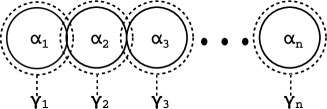
Figure 1: Resolved fiber for $A_{n}$. The curves $\alpha$ corresponding to root vectors are in solid lines while the monodromy invariant fibers $\gamma$ corresponding to coroots are in dotted lines.

$I^{*}_{n-4}$ fibers give the $D_{n}$ Lie algebra. The tree of blown-up rational curves of the resolved $I^{*}_{n-4}$ fiber is depicted in figure 2. The intersection matrices are given by

$$(\gamma_{I}\cdot\gamma_{J})=(\gamma_{I}\cdot\alpha_{J})=\begin{pmatrix}-2&0&1&0&\cdots&0&0\\ 0&-2&1&0&\cdots&0&0\\ 1&1&-2&1&\cdots&0&0\\ 0&0&1&-2&\cdots&0&0\\ \vdots&\vdots&\vdots&\vdots&\ddots&\vdots&\vdots\\ 0&0&0&0&\cdots&-2&1\\ 0&0&0&0&\cdots&1&-2\end{pmatrix}=-C_{IJ}=-{\cal C}_{IJ}\,.$$ (112)

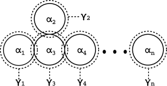
Figure 2: Resolved fiber for $D_{n}$.

The fibers $IV^{*}$, $III^{*}$ and $II^{*}$ give the $E_{6}$, $E_{7}$ and $E_{8}$ Lie algebra respectively. The tree of blown-up rational curves of the resolved $E_{n}$ fiber is depicted in figure 3. The intersection matrices are given by

$$(\gamma_{I}\cdot\gamma_{J})=(\gamma_{I}\cdot\alpha_{J})=\begin{pmatrix}-2&1&0&0&0&\cdots&0&0\\ 1&-2&0&1&0&\cdots&0&0\\ 0&0&-2&1&0&\cdots&0&0\\ 0&1&1&-2&1&\cdots&0&0\\ 0&0&0&1&-2&\cdots&0&0\\ \vdots&\vdots&\vdots&\vdots&\vdots&\ddots&\vdots&\vdots\\ 0&0&0&0&0&\cdots&-2&1\\ 0&0&0&0&0&\cdots&1&-2\end{pmatrix}=-C_{IJ}=-{\cal C}_{IJ}\,.$$ (113)

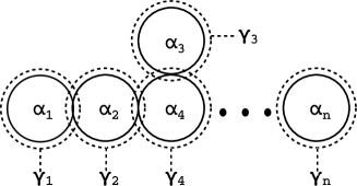
Figure 3: Resolved fiber for $E_{n}$.

$\mathfrak{su}(2)$ can come from an $I_{3}$ or $IV$ fiber with a ${\mathbb{{Z}}}_{2}$ monodromy. The resolved fiber that gives the $A_{1}$ Lie algebra in this way is given by figure 4. The ${\mathbb{{Z}}}_{2}$ interchanges the two ${\mathbb{{P}}}^{1}$’s drawn in the figure, and hence the point where the two rational curves touch is singular. $\gamma_{1}$ is the monodromy invariant fiber. It is shown in [10] that the BPS states come from branes wrapping $\alpha_{1}$ rather than the the individual components drawn as spheres in the figure. The intersection matrices are given by

$$(\gamma_{I}\cdot\gamma_{J})=(\gamma_{I}\cdot\alpha_{J})=\begin{pmatrix}-2\end{pmatrix}=-C_{IJ}=-{\cal C}_{IJ}\,.$$ (114)

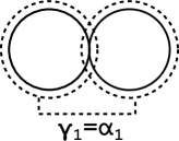
Figure 4: Resolved fiber for $A_{1}$.

A.2.2 Non-simply Laced Lie Algebras

For non-simply laced Lie algebras, the blown-up singular fibers have non-trivial monodromy. The blown-up rational curves form the Dynkin diagram of a larger Lie algebra. Under monodromy, the rational curves are exchanged among themselves. For each fiber, we denote the independent rational curves $\alpha_{I}$, and the monodromy invariant components of the fiber $\gamma_{I}$ . Let us verify that the resolved fibers that give the $A,D,E$ algebra satisfy (107).

The fibers $I^{*}_{(n-3)}$ with ${\mathbb{{Z}}}_{2}$ monodromy give the $B_{n}$ Lie algebra. The tree of blown-up rational curves of the resolved $I^{*}_{(n-3)}$ fiber is depicted in figure 5. The ${\mathbb{{Z}}}_{2}$ monodromy exchanges the two rational curves in $\gamma_{n}$. The intersection matrices are given by

$$\begin{split}(\gamma_{I}\cdot\gamma_{J})=\begin{pmatrix}-2&1&\cdots&0&0&0\\ 1&-2&\cdots&0&0&0\\ \vdots&\vdots&\ddots&\vdots&\vdots&\vdots\\ 0&0&\cdots&-2&1&0\\ 0&0&\cdots&1&-2&2\\ 0&0&\cdots&0&2&-4\end{pmatrix}\,,~{}~{}(\gamma_{I}\cdot\alpha_{J})=\begin{pmatrix}-2&1&\cdots&0&0&0\\ 1&-2&\cdots&0&0&0\\ \vdots&\vdots&\ddots&\vdots&\vdots&\vdots\\ 0&0&\cdots&-2&1&0\\ 0&0&\cdots&1&-2&1\\ 0&0&\cdots&0&2&-2\end{pmatrix}\\[3.0pt] \Rightarrow(\gamma_{I}\cdot\gamma_{J})=-{\cal C}_{IJ},\quad(\gamma_{I}\cdot\alpha_{J})=-C_{IJ}\,.\end{split}$$ (115)

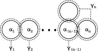
Figure 5: Resolved fiber for $B_{n}$. The curves $\alpha$ corresponding to root vectors are in solid lines while the monodromy invariant fibers $\gamma$ corresponding to coroots are in dotted lines.

The fibers $I_{2n}$ or $I_{(2n+1)}$ with ${\mathbb{{Z}}}_{2}$ monodromy give the $C_{n}$ Lie algebra. The trees of blown-up rational curves of the resolved $I_{2n}$ and $I_{(2n+1)}$ fibers are depicted in figure 6. The ${\mathbb{{Z}}}_{2}$ monodromy exchanges the two rational curves in each $\gamma_{I}$. Just as with the case of $\mathfrak{su}(2)$, $\alpha_{1}$ should be taken to be equal to $\gamma_{1}$ [10]. The intersection matrices are given by

$$\begin{split}(\gamma_{I}\cdot\gamma_{J})=\begin{pmatrix}-2&2&0&\cdots&0&0\\ 2&-4&2&\cdots&0&0\\ 0&2&-4&\cdots&0&0\\ \vdots&\vdots&\vdots&\ddots&\vdots&\vdots\\ 0&0&0&\cdots&-4&2\\ 0&0&0&\cdots&2&-4\end{pmatrix}\,,\quad(\gamma_{I}\cdot\alpha_{J})=\begin{pmatrix}-2&1&0&\cdots&0&0\\ 2&-2&1&\cdots&0&0\\ 0&1&-2&\cdots&0&0\\ \vdots&\vdots&\vdots&\ddots&\vdots&\vdots\\ 0&0&0&\cdots&-2&1\\ 0&0&0&\cdots&1&-2\end{pmatrix}\\[3.0pt] \Rightarrow(\gamma_{I}\cdot\gamma_{J})=-{\cal C}_{IJ},\quad(\gamma_{I}\cdot\alpha_{J})=-C_{IJ}\,.\end{split}$$ (116)

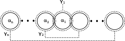
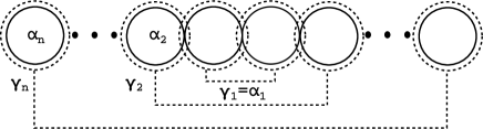
Figure 6: Resolved fiber for $C_{n}$.

The fiber $IV^{*}$ with ${\mathbb{{Z}}}_{2}$ monodromy gives the $F_{4}$ Lie algebra. The tree of blown-up rational curves of the resolved $IV^{*}$ fiber is depicted in figure 7. The ${\mathbb{{Z}}}_{2}$ monodromy exchanges the two rational curves in $\gamma_{3}$ and $\gamma_{4}$. The intersection matrices are given by

$$(\gamma_{I}\cdot\gamma_{J})=\begin{pmatrix}-2&1&0&0\\ 1&-2&2&0\\ 0&2&-4&2\\ 0&0&2&-4\\ \end{pmatrix}=-{\cal C}_{IJ}\,,~{}~{}(\gamma_{I}\cdot\alpha_{J})=\begin{pmatrix}-2&1&0&0\\ 1&-2&1&0\\ 0&2&-2&1\\ 0&0&1&-2\\ \end{pmatrix}=-C_{IJ}\,.$$ (117)

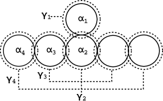
Figure 7: Resolved fiber for $F_{4}$.

The fiber $I^{*}_{0}$ with ${\mathbb{{Z}}}_{3}$ or $\mathfrak{S}_{3}$ monodromy gives the $G_{2}$ Lie algebra. The tree of blown-up rational curves of the resolved $I^{*}_{0}$ fiber is depicted in figure 8. The ${\mathbb{{Z}}}_{3}$ or $\mathfrak{S}_{3}$ monodromy exchanges the three rational curves in $\gamma_{2}$. The intersection matrices are given by

$$(\gamma_{I}\cdot\gamma_{J})=\begin{pmatrix}-2&3\\ 3&-6\end{pmatrix}=-{\cal C}_{IJ}\,,\quad(\gamma_{I}\cdot\alpha_{J})=\begin{pmatrix}-2&1\\ 3&-2\end{pmatrix}=-C_{IJ}\,.$$ (118)

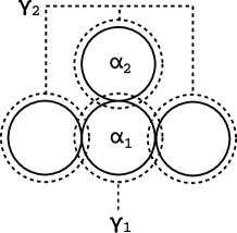
Figure 8: Resolved fiber for $G_{2}$.

Appendix B Proof of Intersection Equations for $\SS_{n}$ of Type S or C

We prove the intersection equations

$$\begin{split}&\pi(\SS_{1}\cdot\SS_{2})\cdot\pi(\SS_{3}\cdot\SS_{4})+\pi(\SS_{1}\cdot\SS_{3})\cdot\pi(\SS_{2}\cdot\SS_{4})+\pi(\SS_{1}\cdot\SS_{4})\cdot\pi(\SS_{2}\cdot\SS_{3})\\ &=\sum_{r}(c_{r}\cdot\SS_{1})(c_{r}\cdot\SS_{2})(c_{r}\cdot\SS_{3})(c_{r}\cdot\SS_{4})+\sum_{\rho}(2g_{\rho}-2)(\chi_{\rho}\cdot\SS_{1})(\chi_{\rho}\cdot\SS_{2})(\chi_{\rho}\cdot\SS_{3})(\chi_{\rho}\cdot\SS_{4})\end{split}$$ (119)

and

$$\begin{split}6K\cdot\pi(\SS_{1}\cdot\SS_{2})=\sum_{r}(c_{r}\cdot\SS_{1})(c_{r}\cdot\SS_{2})+\sum_{\rho}(2g_{\rho}-2)(\chi_{\rho}\cdot\SS_{1})(\chi_{\rho}\cdot\SS_{2})\end{split}$$ (120)

when

$$\SS_{n}\in\{T_{I,\kappa},S_{i}\}\,.$$ (121)

We first check the case when $\SS_{n}$ are all of type S, then check the case when $\SS_{n}$ are all of type C. Finally we check the case when there is a mixture of type S and C cycles among $\SS_{n}$. We refer to the first equation (119) the quartic equation and the second equation (120) the quadratic equation throughout this appendix.

B.1 Type S Cycles Only

Take $\SS_{n}$ to be type S cycles $\{S_{i},S_{j},S_{k},S_{l}\}$. $\SS_{n}$ are dual to abelian vector multiplets. Then using the result (70)

$$b_{ij}=-\pi(S_{i}\cdot S_{j})\,,$$ (122)

the last equation of (24) can be rewritten in the form

$$\begin{split}\pi(S_{i}\cdot S_{j})\cdot\pi(S_{k}\cdot S_{l})+\pi(S_{i}\cdot S_{k})\cdot\pi(S_{j}\cdot S_{l})+\pi(S_{i}\cdot S_{l})\cdot\pi(S_{j}\cdot S_{k})=\sum_{x}q^{x}_{i}q^{x}_{j}q^{x}_{k}q^{x}_{l}\,.\end{split}$$ (123)

We have used $x$ to index all the hypermultiplets in the theory and $q^{x}_{n}$ denotes the charge of hypermultiplet $x$ under the $U(1)$ vector field dual to $S_{n}$.

We note that all hypermultiplets charged under these vector multiplets come from M2 branes wrapping type I curves, which are precisely $c_{r}$. Recall that

$$S_{j}\cdot\chi_{\rho}=0$$ (124)

for all $\rho$ by the construction of S-type cycles.

Then since the charge of the hypermultiplet coming from wrapping branes on $c_{r}$ under vector field $n$ is $c_{r}\cdot S_{i}$, the last equation of (24) is indeed equivalent to the equation

$$\begin{split}&\pi(S_{i}\cdot S_{j})\cdot\pi(S_{k}\cdot S_{l})+\pi(S_{i}\cdot S_{k})\cdot\pi(S_{j}\cdot S_{l})+\pi(S_{i}\cdot S_{l})\cdot\pi(S_{j}\cdot S_{k})\\ &=\sum_{r}(c_{r}\cdot S_{i})(c_{r}\cdot S_{j})(c_{r}\cdot S_{k})(c_{r}\cdot S_{l})+\sum_{\rho}(2g_{\rho}-2)(\chi_{\rho}\cdot S_{i})(\chi_{\rho}\cdot S_{j})(\chi_{\rho}\cdot S_{k})(\chi_{\rho}\cdot S_{l})\end{split}$$ (125)

since the latter term on the right hand side is zero.

Similarly, since the vector $a$ is identified with the canonical class of the base $K$, the second equation in (22) implies that

$$\begin{split}6K\cdot\pi(S_{i}\cdot S_{j})&=-6a\cdot b_{ij}=\sum_{x}q^{x}_{i}q^{x}_{j}\\ &=\sum_{r}(c_{r}\cdot S_{i})(c_{r}\cdot S_{j})+\sum_{\rho}(2g_{\rho}-2)(\chi_{\rho}\cdot S_{i})(\chi_{\rho}\cdot S_{j})\end{split}$$ (126)

for two type S four-cycles $S_{i},S_{j}$. Hence we have shown that (119) and (120) hold when $\SS_{n}$ are all of type S.

B.2 Type C Cycles Only

We prove

$$\begin{split}\pi(T_{I,\kappa}\cdot T_{J,\nu})\cdot&\pi(T_{K,\lambda}\cdot T_{L,\mu})+\text{(2 other groupings)}\\ &=\sum_{r}(c_{r}\cdot T_{I,\kappa})(c_{r}\cdot T_{J,\nu})(c_{r}\cdot T_{K,\lambda})(c_{r}\cdot T_{L,\mu})\\ &+\sum_{\rho}(2g_{\rho}-2)(\chi_{\rho}\cdot T_{I,\kappa})(\chi_{\rho}\cdot T_{J,\nu})(\chi_{\rho}\cdot T_{K,\lambda})(\chi_{\rho}\cdot T_{L,\mu})\end{split}$$ (127)

and

$$\begin{split}6K\cdot\pi(T_{I,\kappa}\cdot T_{J,\nu})=\sum_{r}(c_{r}\cdot T_{I,\kappa})(c_{r}\cdot T_{J,\nu})+\sum_{\rho}(2g_{\rho}-2)(\chi_{\rho}\cdot T_{I,\kappa})(\chi_{\rho}\cdot T_{J,\nu})\end{split}$$ (128)

for $T_{I,\kappa}$ of type C. The quartic equation is only non-trivial when the $\kappa,\nu,\lambda,\mu$ are equal in pairs—this includes the case when they are all equal. The quadratic equation is only non-trivial when $\kappa$ and $\nu$ are equal.

The two statements above follow from three facts.

1. $\pi(T_{I,\kappa}\cdot T_{J,\nu})$ satisfies

   $$\pi(T_{I,\kappa}\cdot T_{J,\nu})=-\delta_{\kappa\nu}b_{\kappa}{\cal C}_{IJ,\kappa}\,,$$ (129)

   so the left-hand side of the quartic equation is zero unless $\kappa,\nu,\lambda,\mu$ are equal in pairs. Similarly, the left hand side of the quadratic equation is zero unless $\kappa$ and $\nu$ are equal.

2. Unless $\kappa,\nu,\lambda,\mu$ are equal in pairs,

   $$\sum_{r}(c_{r}\cdot T_{I,\kappa})(c_{r}\cdot T_{J,\nu})(c_{r}\cdot T_{K,\lambda})(c_{r}\cdot T_{L,\mu})=\sum_{R}k_{R}{\rm tr}_{R}\mathcal{T}_{M,\eta}=0$$ (130)

   for some constants $k_{R}$ and $M,\eta$. Similarly, unless $\kappa$ and $\nu$ are equal,

   $$\sum_{r}(c_{r}\cdot T_{I,\kappa})(c_{r}\cdot T_{J,\nu})=\sum_{R}k_{R}{\rm tr}_{R}\mathcal{T}_{M,\eta}=0$$ (131)

   for some constants $k_{R}$ and $M,\eta$. This is because the hypermultiplets coming from type I cycles always can be organized into representations of the Lie algebra.

3. $\chi_{\rho}$ can be organized into positive(or negative, depending on convention) roots of the simple Lie algebra factors as $\{\chi_{\rho}\}=\{\chi_{s,\kappa}\}$. Any $\chi_{s,\kappa}$ for a given $\kappa$ is a linear combination of curves $\chi_{I,\kappa}$ corresponding to the simple roots of $\mathcal{G}_{\kappa}$. Since

   $$\chi_{I,\kappa}\cdot T_{J,\nu}=-\delta_{\kappa\nu}C_{IJ,\kappa}\,,$$ (132)

   the equation

   $$(\chi_{\rho}\cdot T_{I,\kappa})(\chi_{\rho}\cdot T_{I,\nu})=0$$ (133)

   holds for $\kappa\neq\nu$.

Therefore (127) is non-trivial only when $\kappa,\nu,\lambda,\mu$ are equal in pairs, and (128) is non-trivial only when $\kappa=\nu$.

Now let us write the anomaly equations in a form more convenient to our purposes. The anomaly equations concerning only non-abelian gauge group factors implies that the following holds for all elements ${T_{\kappa}},{T_{\nu}}$ of the Cartan of the gauge groups $\mathcal{G}_{\kappa},\mathcal{G}_{\nu}$:

$$a\cdot{b_{\kappa}}{{\rm tr}{T_{\kappa}}^{2}\over\lambda_{\kappa}} ={1\over 6}({\rm tr}_{\text{Adj}_{\kappa}}{T_{\kappa}}^{2}-\sum_{I}x_{R}{\rm tr}_{R}{T_{\kappa}}^{2})$$ (134)

$$b_{\kappa}\cdot b_{\kappa}({{\rm tr}{T_{\kappa}}^{2}\over\lambda_{\kappa}})^{2} ={1\over 3}(\sum_{I}x_{R}{\rm tr}_{R}{T_{\kappa}}^{4}-{\rm tr}_{\text{Adj}_{\kappa}}{T_{\kappa}}^{4})$$ (135)

$$b_{\kappa}\cdot b_{\nu}({{\rm tr}{T_{\kappa}}^{2}\over\lambda_{\kappa}})({{\rm tr}{T_{\nu}}^{2}\over\lambda_{\nu}}) =\sum_{R,S}x_{RS}{\rm tr}_{R}{T_{\kappa}}^{2}{\rm tr}_{S}{T_{\nu}}^{2}\quad(\kappa\neq\nu)$$ (136)

Let us take ${T_{\kappa}}=t_{I}{\mathcal{T}_{I,\kappa}}$ and ${T_{\nu}}=s_{I}{\mathcal{T}_{I,\kappa}}$ where $I$ runs over the indices of the coroot basis of the Cartan sub-algebra of each gauge group. Expanding the equalities above, we obtain polynomials with respect to $t_{I}$ and $s_{I}$ on both sides of the equations. The anomaly equations must hold for any value of $t_{I}$ and $s_{I}$. Hence all the coefficients of the polynomials must be identical. By identifying the coefficients, we obtain

$$\begin{split}a\cdot{b_{\kappa}}{\cal C}_{IJ,\kappa}&={1\over 6}({\rm tr}_{\text{Adj}_{\kappa}}{\mathcal{T}_{I,\kappa}}{\mathcal{T}_{J,\kappa}}-\sum_{I}x_{R}{\rm tr}_{R}{\mathcal{T}_{I,\kappa}}{\mathcal{T}_{J,\kappa}})\\ b_{\kappa}\cdot b_{\kappa}({\cal C}_{IJ,\kappa}{\cal C}_{KL,\kappa}+&{\cal C}_{IK,\kappa}{\cal C}_{JL,\kappa}+{\cal C}_{IL,\kappa}{\cal C}_{JK,\kappa})=\\ &\sum_{I}x_{R}{\rm tr}_{R}{\mathcal{T}_{I,\kappa}}{\mathcal{T}_{J,\kappa}}{\mathcal{T}_{K,\kappa}}{\mathcal{T}_{L,\kappa}}-{\rm tr}_{\text{Adj}_{\kappa}}{\mathcal{T}_{I,\kappa}}{\mathcal{T}_{J,\kappa}}{\mathcal{T}_{K,\kappa}}{\mathcal{T}_{L,\kappa}}\\ b_{\kappa}\cdot b_{\nu}{\cal C}_{IJ,\kappa}{\cal C}_{KL,\nu}&=\sum_{R,S}x_{RS}{\rm tr}_{R}{\mathcal{T}_{I,\kappa}}{\mathcal{T}_{J,\kappa}}{\rm tr}_{S}{\mathcal{T}_{K,\nu}}{\mathcal{T}_{L,\nu}}\end{split}$$ (137)

for $\kappa\neq\nu$.

We can write all the elements of the right-hand sides as a sum of products of the charge of each vector or hypermultiplet under each Cartan element. Each charged multiplet corresponds to a type I or a type F rational curve, and its charges are given by the intersection numbers of the curve with the four-cycles of type C. Rewriting the right-hand sides of the equations we obtain

$$\begin{split}-6a\cdot{b_{\kappa}}&{\cal C}_{IJ,\kappa}=\\ &\sum_{r}(c_{r}\cdot T_{I,\kappa})(c_{r}\cdot T_{J,\kappa})+\sum_{\rho}(2g_{\rho}-2)(\chi_{\rho}\cdot T_{I,\kappa})(\chi_{\rho}\cdot T_{J,\kappa})\\ b_{\kappa}\cdot b_{\kappa}({\cal C}_{IJ,\kappa}{\cal C}_{KL,\kappa}&+{\cal C}_{IK,\kappa}{\cal C}_{JL,\kappa}+{\cal C}_{IL,\kappa}{\cal C}_{JK,\kappa})=\\ &\sum_{r}(c_{r}\cdot T_{I,\kappa})(c_{r}\cdot T_{J,\kappa})(c_{r}\cdot T_{K,\kappa})(c_{r}\cdot T_{L,\kappa})\\ &+\sum_{\rho}(2g_{\rho}-2)(\chi_{\rho}\cdot T_{I,\kappa})(\chi_{\rho}\cdot T_{J,\kappa})(\chi_{\rho}\cdot T_{K,\kappa})(\chi_{\rho}\cdot T_{L,\kappa})\\ b_{\kappa}\cdot b_{\nu}&{\cal C}_{IJ,\kappa}{\cal C}_{KL,\nu}=\\ &\sum_{r}(c_{r}\cdot T_{I,\kappa})(c_{r}\cdot T_{J,\kappa})(c_{r}\cdot T_{K,\nu})(c_{r}\cdot T_{L,\nu})\\ &+\sum_{\rho}(2g_{\rho}-2)(\chi_{\rho}\cdot T_{I,\kappa})(\chi_{\rho}\cdot T_{J,\kappa})(\chi_{\rho}\cdot T_{K,\nu})(\chi_{\rho}\cdot T_{L,\nu})\end{split}$$ (138)

Note that the curve $\chi_{\rho}$ contributes $2g_{\rho}$ hypermultiplets and two vector multiplets [13, 23], as explained in section 3.2.1. The vector multiplet always contributes with a negative sign with respect to the contribution of the hypermultiplet to the right hand sides of the equations. The last term of the last equation is zero.

Finally using

$$\pi(T_{I,\kappa}\cdot T_{J,\nu})=-\delta_{\kappa\nu}b_{\kappa}{\cal C}_{IJ,\kappa}\,,$$ (139)

and the fact that $a$ is equal to the canonical class $K$ of the base, the three equations translate into

$$\begin{split}6K&\cdot\pi(T_{I,\kappa}\cdot T_{J,\kappa})=\\ &\sum_{r}(c_{r}\cdot T_{I,\kappa})(c_{r}\cdot T_{J,\kappa})+\sum_{\rho}(2g_{\rho}-2)(\chi_{\rho}\cdot T_{I,\kappa})(\chi_{\rho}\cdot T_{J,\kappa})\\ \pi(T_{I,\kappa}\cdot T_{J,\kappa})\cdot&\pi(T_{K,\kappa}\cdot T_{L,\kappa})+\text{(2 other groupings)}=\\ &\sum_{r}(c_{r}\cdot T_{I,\kappa})(c_{r}\cdot T_{J,\kappa})(c_{r}\cdot T_{K,\kappa})(c_{r}\cdot T_{L,\kappa})\\ &+\sum_{\rho}(2g_{\rho}-2)(\chi_{\rho}\cdot T_{I,\kappa})(\chi_{\rho}\cdot T_{J,\kappa})(\chi_{\rho}\cdot T_{K,\kappa})(\chi_{\rho}\cdot T_{L,\kappa})\\ \pi(T_{I,\kappa}\cdot T_{J,\kappa})\cdot&\pi(T_{K,\nu}\cdot T_{L,\nu})+\text{(2 other groupings)}=\\ &\sum_{r}(c_{r}\cdot T_{I,\kappa})(c_{r}\cdot T_{J,\kappa})(c_{r}\cdot T_{K,\nu})(c_{r}\cdot T_{L,\nu})\\ &+\sum_{\rho}(2g_{\rho}-2)(\chi_{\rho}\cdot T_{I,\kappa})(\chi_{\rho}\cdot T_{J,\kappa})(\chi_{\rho}\cdot T_{K,\nu})(\chi_{\rho}\cdot T_{L,\nu})\end{split}$$ (140)

We note that in the last equation, the two other groupings of cycles that are not written down are zero.

B.3 Both Type S and C Cycles

The quadratic equation is always trivial when $\SS_{1}$ and $\SS_{2}$ are each of type S and C, for the following reasons.

1. The left hand side of the quadratic equation is trivially zero since

   $$\pi(S_{i}\cdot T_{I,\kappa})=0\,,$$ (141)

   due to the construction of type S cycles.

2. The hypermultiplets come in representations of the non-abelian Lie algebra. Hence,

   $$\sum_{r}(c_{r}\cdot S_{i})(c_{r}\cdot T_{I,\kappa})=\sum_{R}k_{R}{\rm tr}_{R}\mathcal{T}_{I,\kappa}=0\,.$$ (142)

3. $S_{i}$ do not intersect type $\chi_{\rho}$ curves by construction. Hence,

   $$\sum_{\rho}(2g_{\rho}-2)(\chi_{\rho}\cdot S_{i})(\chi_{\rho}\cdot T_{I,\kappa})=0\,.$$ (143)

Similarly we can show that the non-trivial cases to check for the quartic equation are, without loss of generality, when

1. $\SS_{1}={\mathcal{T}_{I,\kappa}},~{}\SS_{2}={\mathcal{T}_{J,\kappa}},~{}\SS_{3}={\mathcal{T}_{K,\kappa}},~{}\SS_{4}=S_{i}$.

2. $\SS_{1}={\mathcal{T}_{I,\kappa}},~{}\SS_{2}={\mathcal{T}_{J,\kappa}},~{}\SS_{3}=S_{i},~{}\SS_{4}=S_{j}$.

From the anomaly equations, we can show that for any element of the Cartan $T_{\kappa}$ of $\mathcal{G}_{\kappa}$

$$\begin{split}0&=\sum_{R,q_{i}}x_{R,q_{i}}q_{i}{\rm tr}_{R}T_{\kappa}^{3}\\ b_{\kappa}\cdot b_{ij}{{\rm tr}T_{\kappa}^{2}\over\lambda_{\kappa}}&=\sum_{R,q_{i},q_{j}}x_{R,q_{i},q_{j}}q_{i}q_{j}{\rm tr}T_{\kappa}^{2}\end{split}$$ (144)

Setting $T_{\kappa}={\mathcal{T}_{I,\kappa}}t_{I}$, we can write both sides of the two equations as polynomials with respect to $t_{I}$. Since the equality must hold for all values of $t_{I}$, the coefficients of the polynomials must match on both sides, and hence

$$\begin{split}0&=\sum_{R,q_{i}}x_{R,q_{i}}{\rm tr}_{R}({\mathcal{T}_{I,\kappa}}{\mathcal{T}_{J,\kappa}}{\mathcal{T}_{L,\kappa}})q_{i}\\ b_{\kappa}\cdot b_{ij}{\cal C}_{IJ}&=\sum_{R,q_{i},q_{j}}x_{R,q_{i},q_{j}}{\rm tr}_{R}({\mathcal{T}_{I,\kappa}}{\mathcal{T}_{J,\kappa}})q_{i}q_{j}\end{split}$$ (145)

As before, we can write all the elements of the right-hand sides as a sum of products of the charge of each vector or hypermultiplet under $\mathcal{T}_{I,\kappa}$, $U(1)_{i}$ or $U(1)_{j}$. Each charged hypermultiplet has a corresponding type I rational curve, and its charge is given by the intersection numbers of the curve with the four-cycles of type C or S. Rewriting the right-hand sides of the equations we obtain

$$\begin{split}0&=\sum_{r}(c_{r}\cdot T_{I,\kappa})(c_{r}\cdot T_{J,\kappa})(c_{r}\cdot T_{K,\kappa})(c_{r}\cdot S_{i})\\ b_{\kappa}\cdot b_{ij}{\cal C}_{IJ,\kappa}&=\sum_{r}(c_{r}\cdot T_{I,\kappa})(c_{r}\cdot T_{J,\kappa})(c_{r}\cdot S_{i})(c_{r}\cdot S_{j})\end{split}$$ (146)

Using

$$b_{\kappa}{\cal C}_{IJ,\kappa}=-\pi({\mathcal{T}_{I,\kappa}}\cdot{\mathcal{T}_{J,\kappa}}),\quad\pi({\mathcal{T}_{I,\kappa}}\cdot S_{i})=0,\quad b_{ij}=-\pi(S_{i}\cdot S_{j})\,,$$ (147)

we obtain the final expressions by rewriting the equations:

$$\begin{split}\pi({\mathcal{T}_{I,\kappa}}\cdot S_{i})\cdot\pi({\mathcal{T}_{J,\kappa}}\cdot{\mathcal{T}_{L,\kappa}})&+\text{(2 other groupings)}\\ &=\sum_{r}(c_{r}\cdot T_{I,\kappa})(c_{r}\cdot T_{J,\kappa})(c_{r}\cdot T_{K,\kappa})(c_{r}\cdot S_{i})\\ &+\sum_{\rho}(2g_{\rho}-2)(\chi_{\rho}\cdot T_{I,\kappa})(\chi_{\rho}\cdot T_{J,\kappa})(\chi_{\rho}\cdot T_{K,\kappa})(\chi_{\rho}\cdot S_{i})\\ \pi({\mathcal{T}_{I,\kappa}}\cdot{\mathcal{T}_{J,\kappa}})\cdot\pi(S_{i}\cdot S_{j})&+\text{(2 other groupings)}\\ &=\sum_{r}(c_{r}\cdot T_{I,\kappa})(c_{r}\cdot T_{J,\kappa})(c_{r}\cdot S_{i})(c_{r}\cdot S_{j})\\ &+\sum_{\rho}(2g_{\rho}-2)(\chi_{\rho}\cdot T_{I,\kappa})(\chi_{\rho}\cdot T_{J,\kappa})(\chi_{\rho}\cdot S_{i})(\chi_{\rho}\cdot S_{j})\end{split}$$ (148)

Note that the left hand side of the first equation is zero, and that the two other groupings in the second equation are zero. The second term on the right hand side of both equations are zero since $S_{i}\cdot\chi_{\rho}=0$ by construction of type S cycles. $\Box$

References

- [1] S. L. Adler, “Axial vector vertex in spinor electrodynamics,” Phys. Rev. 177, 2426 (1969). J. S. Bell and R. Jackiw, “A PCAC puzzle: pi0 gamma gamma in the sigma model,” Nuovo Cim. A 60, 47 (1969).
- [2] L. Alvarez-Gaume and E. Witten, “Gravitational Anomalies,” Nucl. Phys. B 234, 269 (1984).
- [3] M. B. Green, J. H. Schwarz, P. C. West, “Anomaly Free Chiral Theories in Six-Dimensions,” Nucl. Phys. B254, 327-348 (1985).
- [4] A. Sagnotti, “A Note on the Green-Schwarz mechanism in open string theories,” Phys. Lett. B 294, 196 (1992) [arXiv:hep-th/9210127].
- [5] V. Sadov, “Generalized Green-Schwarz mechanism in F theory,” Phys. Lett. B388, 45-50 (1996). [hep-th/9606008].
- [6] M. B. Green, J. H. Schwarz, “Anomaly Cancellation in Supersymmetric D=10 Gauge Theory and Superstring Theory,” Phys. Lett. B149, 117-122 (1984).
- [7] C. Vafa, “Evidence for F theory,” Nucl. Phys. B469, 403-418 (1996). [hep-th/9602022].
- [8] D. R. Morrison, C. Vafa, “Compactifications of F theory on Calabi-Yau threefolds. 1,” Nucl. Phys. B473, 74-92 (1996), [hep-th/9602114].
- [9] D. R. Morrison, C. Vafa, “Compactifications of F theory on Calabi-Yau threefolds. 2.,” Nucl. Phys. B476, 437-469 (1996). [hep-th/9603161].
- [10] P. S. Aspinwall, S. H. Katz, D. R. Morrison, “Lie groups, Calabi-Yau threefolds, and F theory,” Adv. Theor. Math. Phys. 4, 95-126 (2000). [hep-th/0002012].
- [11] A. Grassi, D. R. Morrison, “Group representations and the Euler characteristic of elliptically fibered Calabi-Yau threefolds,” [math/0005196 [math-ag]].
- [12] A. Grassi, D. R. Morrison, “Anomalies and the Euler characteristic of elliptic Calabi-Yau threefolds,” [arXiv:1109.0042 [hep-th]].
- [13] E. Witten, “Phase transitions in M theory and F theory,” Nucl. Phys. B471, 195-216 (1996). [hep-th/9603150].
- [14] P. S. Aspinwall, D. R. Morrison, “Point - like instantons on K3 orbifolds,” Nucl. Phys. B503, 533-564 (1997). [hep-th/9705104].
- [15] E. Witten, “Some comments on string dynamics,” [hep-th/9507121].
- [16] A. Strominger, “Open p-branes,” Phys. Lett. B383, 44-47 (1996). [hep-th/9512059].
- [17] M. J. Duff, R. Minasian, E. Witten, “Evidence for heterotic / heterotic duality,” Nucl. Phys. B465, 413-438 (1996). [hep-th/9601036].
- [18] O. J. Ganor, A. Hanany, “Small E(8) instantons and tensionless noncritical strings,” Nucl. Phys. B474, 122-140 (1996). [hep-th/9602120].
- [19] N. Seiberg, E. Witten, “Comments on string dynamics in six-dimensions,” Nucl. Phys. B471, 121-134 (1996). [hep-th/9603003].
- [20] M. J. Duff, H. Lu, C. N. Pope, “Heterotic phase transitions and singularities of the gauge dyonic string,” Phys. Lett. B378, 101-106 (1996). [hep-th/9603037].
- [21] W. Fulton, Intersection Theory, Springer Verlag, 1984.
- [22] P. Griffiths, J. Harris, Principles of Algebraic Geometry, John Wiley & Sons, Inc., New York, 1978.
- [23] S. H. Katz, D. R. Morrison, M. R. Plesser, “Enhanced gauge symmetry in type II string theory,” Nucl. Phys. B477, 105-140 (1996). [arXiv:hep-th/9601108 [hep-th]].
- [24] S. Ferrara, R. Minasian, A. Sagnotti, “Low-energy analysis of M and F theories on Calabi-Yau threefolds,” Nucl. Phys. B474, 323-342 (1996). [hep-th/9604097].
- [25] T. W. Grimm, “The N=1 effective action of F-theory compactifications,” Nucl. Phys. B845, 48-92 (2011). [arXiv:1008.4133 [hep-th]].
- [26] T. W. Grimm and H. Hayashi, “F-theory fluxes, Chirality and Chern-Simons theories,” arXiv:1111.1232 [hep-th].
- [27] F. Bonetti, T. Grimm, “Six-dimensional (1,0) action for F-theory via M-theory on Calabi-Yau threefolds,” to appear.
- [28] V. Kumar, W. Taylor, “String Universality in Six Dimensions,” [arXiv:0906.0987 [hep-th]].
- [29] D. S. Park, W. Taylor, “Constraints on 6D Supergravity Theories with Abelian Gauge Symmetry,” [arXiv:1110.5916 [hep-th]].
- [30] V. Kumar, D. R. Morrison and W. Taylor, “Global aspects of the space of 6D N = 1 supergravities,” arXiv:1008.1062 [hep-th].
- [31] F. Riccioni, “Abelian vector multiplets in six-dimensional supergravity,” Phys. Lett. B 474, 79 (2000) [arXiv:hep-th/9910246]. F. Riccioni, “All couplings of minimal six-dimensional supergravity,” Nucl. Phys. B 605, 245 (2001) [arXiv:hep-th/0101074].
- [32] M. Berkooz, R. G. Leigh, J. Polchinski, J. H. Schwarz, N. Seiberg and E. Witten, “Anomalies, Dualities, and Topology of D=6 N=1 Superstring Vacua,” Nucl. Phys. B 475, 115 (1996) [arXiv:hep-th/9605184].
- [33] N. Seiberg, W. Taylor, “Charge Lattices and Consistency of 6D Supergravity,” [arXiv:1103.0019 [hep-th]].
- [34] V. Kumar, D. R. Morrison and W. Taylor, “Mapping 6D N = 1 supergravities to F-theory,” arXiv:0911.3393 [hep-th].
- [35] M. Bershadsky, K. A. Intriligator, S. Kachru, D. R. Morrison, V. Sadov, C. Vafa, “Geometric singularities and enhanced gauge symmetries,” Nucl. Phys. B481, 215-252 (1996). [hep-th/9605200].
- [36] S. H. Katz, C. Vafa, “Matter from geometry,” Nucl. Phys. B497, 146-154 (1997). [hep-th/9606086].
- [37] D. R. Morrison, W. Taylor, “Matter and singularities,” [arXiv:1106.3563 [hep-th]].
- [38] M. Esole, S. -T. Yau, “Small resolutions of SU(5)-models in F-theory,” [arXiv:1107.0733 [hep-th]].
- [39] M. Esole, J. Fullwood, S. -T. Yau, “D5 elliptic fibrations: non-Kodaira fibers and new orientifold limits of F-theory,” [arXiv:1110.6177 [hep-th]].
- [40] J. Marsano, S. Schafer-Nameki, “Yukawas, G-flux, and Spectral Covers from Resolved Calabi-Yau’s,” [arXiv:1108.1794 [hep-th]].
- [41] S. Krause, C. Mayrhofer, T. Weigand, “ flux, chiral matter and singularity resolution in F-theory compactifications,” [arXiv:1109.3454 [hep-th]].
- [42] A. Strominger, “Superstrings with Torsion,” Nucl. Phys. B274, 253 (1986).
- [43] J. Erler, “Anomaly Cancellation In Six-Dimensions,” J. Math. Phys. 35, 1819 (1994) [arXiv:hep-th/9304104].
- [44] G. Aldazabal, A. Font, L. E. Ibanez, A. M. Uranga, “New branches of string compactifications and their F theory duals,” Nucl. Phys. B492, 119-151 (1997) [hep-th/9607121].
- [45] P. Berglund, A. Klemm, P. Mayr, S. Theisen, “On type IIB vacua with varying coupling constant,” Nucl. Phys. B558, 178-204 (1999) [hep-th/9805189].
- [46] P. S. Aspinwall, “An analysis of fluxes by duality,” [hep-th/0504036].
- [47] R. Blumenhagen, G. Honecker, T. Weigand, “Loop-corrected compactifications of the heterotic string with line bundles,” JHEP 0506, 020 (2005). [hep-th/0504232]. R. Blumenhagen, G. Honecker, T. Weigand, “Supersymmetric (non-)Abelian bundles in the Type I and SO(32) heterotic string,” JHEP 0508, 009 (2005). [hep-th/0507041]. R. Blumenhagen, G. Honecker, T. Weigand, “Non-Abelian brane worlds: The Heterotic string story,” JHEP 0510, 086 (2005). [hep-th/0510049]. T. Weigand, “Heterotic vacua from general (non-) Abelian bundles,” Fortsch. Phys. 54, 505-513 (2006). [hep-th/0512191].
- [48] G. Honecker, “Massive U(1)s and heterotic five-branes on K3,” Nucl. Phys. B748, 126-148 (2006) [hep-th/0602101]. G. Honecker, M. Trapletti, “Merging Heterotic Orbifolds and K3 Compactifications with Line Bundles,” JHEP 0701, 051 (2007) [hep-th/0612030]. G. Honecker, “Orbifolds versus smooth heterotic compactifications,” [arXiv:0709.2037 [hep-th]].
- [49] M. Buican, D. Malyshev, D. R. Morrison, H. Verlinde, M. Wijnholt, “D-branes at Singularities, Compactification, and Hypercharge,” JHEP 0701, 107 (2007). [hep-th/0610007].
- [50] H. Hayashi, T. Kawano, Y. Tsuchiya, T. Watari, “More on Dimension-4 Proton Decay Problem in F-theory – Spectral Surface, Discriminant Locus and Monodromy,” Nucl. Phys. B840, 304-348 (2010). [arXiv:1004.3870 [hep-th]].
- [51] T. W. Grimm, T. Weigand, “On Abelian Gauge Symmetries and Proton Decay in Global F-theory GUTs,” Phys. Rev. D82, 086009 (2010). [arXiv:1006.0226 [hep-th]].
- [52] J. Marsano, N. Saulina, S. Schafer-Nameki, “A Note on G-Fluxes for F-theory Model Building,” JHEP 1011, 088 (2010). [arXiv:1006.0483 [hep-th]]. J. Marsano, N. Saulina, S. Schafer-Nameki, “On G-flux, M5 instantons, and U(1)s in F-theory,” [arXiv:1107.1718 [hep-th]].
- [53] J. Marsano, “Hypercharge Flux, Exotics, and Anomaly Cancellation in F-theory GUTs,” Phys. Rev. Lett. 106, 081601 (2011). [arXiv:1011.2212 [hep-th]].
- [54] M. J. Dolan, J. Marsano, N. Saulina, S. Schafer-Nameki, “F-theory GUTs with U(1) Symmetries: Generalities and Survey,” Phys. Rev. D84, 066008 (2011). [arXiv:1102.0290 [hep-th]].
- [55] T. W. Grimm, M. Kerstan, E. Palti, T. Weigand, “Massive Abelian Gauge Symmetries and Fluxes in F-theory,” [arXiv:1107.3842 [hep-th]].
- [56] R. Wazir. “Arithmetic on elliptic threefolds,” Compos. Math. 140, 567-580 (2004).
- [57] K. Hulek and R. Kloosterman, “Calculating the Mordell-Weil rank of elliptic threefolds and the cohomology of singular hypersurfaces,” [arXiv:0806.2025v3].
- [58] F. Denef, “Les Houches Lectures on Constructing String Vacua,” [arXiv:0803.1194 [hep-th]].
- [59] A. C. Cadavid, A. Ceresole, R. D’Auria, S. Ferrara, “Eleven-dimensional supergravity compactified on Calabi-Yau threefolds,” Phys. Lett. B357, 76-80 (1995). [hep-th/9506144].
- [60] I. Antoniadis, S. Ferrara, T. R. Taylor, “N=2 heterotic superstring and its dual theory in five-dimensions,” Nucl. Phys. B460, 489-505 (1996). [arXiv:hep-th/9511108 [hep-th]].
- [61] S. Ferrara, R. R. Khuri, R. Minasian, “M theory on a Calabi-Yau manifold,” Phys. Lett. B375, 81-88 (1996). [hep-th/9602102].
- [62] P. S. Aspinwall, “K3 surfaces and string duality,” [hep-th/9611137].
- [63] J. A. Harvey, G. W. Moore, “Algebras, BPS states, and strings,” Nucl. Phys. B463, 315-368 (1996). [hep-th/9510182]. J. A. Harvey, G. W. Moore, “On the algebras of BPS states,” Commun. Math. Phys. 197, 489-519 (1998). [hep-th/9609017].
- [64] T. Shioda, “Mordell-Weil lattices and Galois representation. I,” Proc. Japan Acad. 65A, 268-271 (1989).
- [65] M. Fukae, Y. Yamada, S. -K. Yang, “Mordell-Weil lattice via string junctions,” Nucl. Phys. B572, 71-94 (2000). [hep-th/9909122].
- [66] Z. Guralnik, “String junctions and nonsimply connected gauge groups,” JHEP 0107, 002 (2001). [hep-th/0102031].
- [67] A. Klemm, B. Lian, S. S. Roan, S. -T. Yau, “Calabi-Yau fourfolds for M theory and F theory compactifications,” Nucl. Phys. B518, 515-574 (1998). [hep-th/9701023].
- [68] S. Sethi, C. Vafa, E. Witten, “Constraints on low dimensional string compactifications,” Nucl. Phys. B480, 213-224 (1996). [hep-th/9606122].
- [69] P. Aluffi, M. Esole, “Chern class identities from tadpole matching in type IIB and F-theory,” JHEP 0903, 032 (2009). [arXiv:0710.2544 [hep-th]].
- [70] J. Fullwood, “On generalized Sethi-Vafa-Witten formulas,” [arXiv:1103.6066 [math.AG]].
- [71] D. J. Gross, J. A. Harvey, E. J. Martinec, R. Rohm, “The Heterotic String,” Phys. Rev. Lett. 54, 502-505 (1985); “Heterotic String Theory. 1. The Free Heterotic String,” Nucl. Phys. B256, 253 (1985); “Heterotic String Theory. 2. The Interacting Heterotic String,” Nucl. Phys. B267, 75 (1986).
- [72] A. Adams, O. DeWolfe and W. Taylor, “String universality in ten dimensions,” Phys. Rev. Lett. 105, 071601 (2010) [arXiv:1006.1352 [hep-th]].
- [73] V. Kumar, W. Taylor, “A Bound on 6D N=1 supergravities,” JHEP 0912, 050 (2009). [arXiv:0910.1586 [hep-th]].
- [74] V. Kumar, D. S. Park, W. Taylor, “6D supergravity without tensor multiplets,” JHEP 1104, 080 (2011). [arXiv:1011.0726 [hep-th]].
- [75] W. Taylor, “TASI Lectures on Supergravity and String Vacua in Various Dimensions,” [arXiv:1104.2051 [hep-th]].
- [76] J. Polchinski, “Monopoles, duality, and string theory,” Int. J. Mod. Phys. A19S1, 145-156 (2004). [hep-th/0304042].
- [77] T. Banks, N. Seiberg, “Symmetries and Strings in Field Theory and Gravity,” Phys. Rev. D83, 084019 (2011). [arXiv:1011.5120 [hep-th]].
- [78] S. Hellerman, E. Sharpe, “Sums over topological sectors and quantization of Fayet-Iliopoulos parameters,” [arXiv:1012.5999 [hep-th]].
- [79] R. Donagi, M. Wijnholt, “Model Building with F-Theory,” [arXiv:0802.2969 [hep-th]]. R. Donagi, M. Wijnholt, “Higgs Bundles and UV Completion in F-Theory,” [arXiv:0904.1218 [hep-th]].
- [80] C. Beasley, J. J. Heckman, C. Vafa, “GUTs and Exceptional Branes in F-theory - I,” JHEP 0901, 058 (2009). [arXiv:0802.3391 [hep-th]]. C. Beasley, J. J. Heckman, C. Vafa, “GUTs and Exceptional Branes in F-theory - II: Experimental Predictions,” JHEP 0901, 059 (2009). [arXiv:0806.0102 [hep-th]].
- [81] H. Hayashi, T. Kawano, R. Tatar, T. Watari, “Codimension-3 Singularities and Yukawa Couplings in F-theory,” Nucl. Phys. B823, 47-115 (2009). [arXiv:0901.4941 [hep-th]].
- [82] R. Blumenhagen, T. W. Grimm, B. Jurke, T. Weigand, “Global F-theory GUTs,” Nucl. Phys. B829, 325-369 (2010). [arXiv:0908.1784 [hep-th]].
- [83] M. Cvetic, I. Garcia-Etxebarria, J. Halverson, “Global F-theory Models: Instantons and Gauge Dynamics,” JHEP 1101, 073 (2011). [arXiv:1003.5337 [hep-th]]. M. Cvetic, J. Halverson, I. Garcia-Etxebarria, “Three Looks at Instantons in F-theory – New Insights from Anomaly Inflow, String Junctions and Heterotic Duality,” [arXiv:1107.2388 [hep-th]].
- [84] A. P. Braun, A. Collinucci, R. Valandro, “G-flux in F-theory and algebraic cycles,” [arXiv:1107.5337 [hep-th]].
- [85] T. Weigand, “Lectures on F-theory compactifications and model building,” Class. Quant. Grav. 27, 214004 (2010). [arXiv:1009.3497 [hep-th]].
- [86] E. Dudas, E. Palti, “On hypercharge flux and exotics in F-theory GUTs,” JHEP 1009, 013 (2010). [arXiv:1007.1297 [hep-ph]].
- [87] H. Georgi, “Lie Algebras In Particle Physics. From Isospin To Unified Theories,” Front. Phys. 54, 1-255 (1982).
- [88] R. N. Cahn, “Semisimple Lie Algebras And Their Representations,” Menlo Park, Usa: Benjamin/cummings ( 1984) 158 P. ( Frontiers In Physics, 59).