Weighted eigenfunction estimates with applications to compressed sensing

Abstract.

Using tools from semiclassical analysis, we give weighted $L^{\infty}$ estimates for eigenfunctions of strictly convex surfaces of revolution. These estimates give rise to new sampling techniques and provide improved bounds on the number of samples necessary for recovering sparse eigenfunction expansions on surfaces of revolution. On the sphere, our estimates imply that any function having an $s$-sparse expansion in the first $N$ spherical harmonics can be efficiently recovered from its values at $m\gtrsim sN^{1/6}\log^{4}(N)$ sampling points.

1. Introduction

Consider the sphere and a chosen rotational action generated by $\partial_{\varphi}$:

$${\mathbb{S}}^{2}:=\{x\in\mathbb{R}^{3}\,:\,x_{1}^{2}+x_{2}^{2}+x_{3}^{2}=1\}\,,\ \ \ \partial_{\varphi}=x_{1}\partial_{x_{2}}-x_{2}\partial_{x_{1}}\,,$$

$$\mathbb{S}^{2}\ni x=(\cos\varphi\sin\theta,\sin\varphi\sin\theta,\cos\theta)\,,\ \ 0\leq\theta\leq\pi\,,\ \ 0\leq\varphi\leq 2\pi\,.$$

Let $k,\ell\in\mathbb{Z}$, $|k|\leq\ell$, and let $Y_{\ell}^{k}(\varphi,\theta)$ be the $L^{2}$ normalized spherical harmonics, the joint eigenfunctions of the Laplacian in spherical coordinates $\Delta_{{\mathbb{S}}^{2}}$ and the rotational generator $\partial_{\varphi}$:

$$\begin{gathered}-\Delta_{{\mathbb{S}}^{2}}Y_{\ell}^{k}=-\left(\frac{1}{\sin^{2}\theta}\partial_{\varphi}^{2}+\frac{1}{\sin\theta}\partial_{\theta}\left(\sin\theta\partial_{\theta}\right)\right)Y_{\ell}^{k}=l(l+1)Y_{\ell}^{k}\,,\ \ \ \frac{1}{i}\partial_{\varphi}Y_{\ell}^{k}=kY_{\ell}^{k}\,,\\ \int_{0}^{2\pi}\int_{0}^{\pi}Y_{\ell}^{k}(\varphi,\theta)\overline{Y_{\ell^{\prime}}^{k^{\prime}}(\varphi,\theta)}\sin\theta d\theta d\varphi=\delta_{\ell\ell^{\prime}}\delta_{kk^{\prime}}\,.\end{gathered}$$ (1.3)

Applied to the sphere, our main result on weighted $L^{\infty}$ estimates reads

Theorem 1.

Let $Y_{\ell}^{k}(\varphi,\theta)$, $0\leq\varphi\leq 2\pi$, $0\leq\theta\leq\pi$, be the spherical harmonics defined above. Then for $\ell\geq 1$,

$$|\sin^{2}\theta\cos\theta|^{1/6}\,|Y_{\ell}^{k}(\varphi,\theta)|\leq C\ell^{1/6}\,,$$ (1.4)

where $C$ is a universal constant.

The power $\ell^{1/6}$ in (1.4) can be explained as follows. Taking the Fourier expansion in $\varphi$ reduces the first differential equation in (1.3) to

$$\left(\frac{1}{\sin\theta}h\partial_{\theta}\left(\sin\theta h\partial_{\theta}\right)+\frac{\alpha^{2}}{\sin^{2}\theta}-1\right)u=0,\ \ h=(\ell(\ell+1))^{-1/2},\ \ \alpha=h^{2}k^{2},$$

where $k\in{\mathbb{Z}}$ is an eigenvalue of $\frac{1}{i}\partial_{\varphi}$ and $Y_{\ell}^{k}=u(\theta)e^{ik\varphi}$. When $\alpha$ is such that $0<\epsilon<|\alpha|<1-\epsilon$, this equation has two turning points at $\sin\theta=\pm\alpha$. Physically this corresponds to caustic formation: the focusing at turning points increases the intensity of the wave function, that is, it increases its $L^{\infty}$ norm by a factor of $h^{-1/6}\sim\ell^{1/6}$ – see Proposition 4.5 below. Since the $h^{-1/6}$ loss happens all over the sphere, such growth in the $L^{\infty}$ norm cannot be eliminated by a weight function. In order to get a uniform bound on the entire sphere in (1.4), we choose a weight function vanishing at the pole and the equator. A more detailed explanation of the weights and the principles of semiclassical analysis on which the analysis is based is given at the end of Section 3.

1.1. Motivation

Consider functions on the sphere which are bandlimited and sparse:

$$f(\varphi,\theta)=\sum_{\ell=0}^{\sqrt{N}-1}\sum_{k=-\ell}^{\ell}c_{\ell,k}Y_{\ell}^{k}(\varphi,\theta);\quad\textrm{at most $s<N$ of the $c_{\ell,k}$ are nonzero.}$$ (1.5)

Functions well-approximated as bandlimited and sparse arise in applications ranging from models for protein structure [20] to cosmic microwave background (CMB) data [1]. In [24], Rauhut and Ward showed that such functions can be efficiently reconstructed from far less information than their ambient dimension suggests; in particular, they show that for certain sets of sampling points $(\varphi_{i},\theta_{i})\in\mathbb{S}^{2},\hskip 2.84526ptj\in[m],$ of size

$$m\gtrsim sN^{1/4}\log^{4}N,$$ (1.6)

any function $f$ of the form (1.5) can be reconstructed from its values $f(\varphi_{i},\theta_{i})$ as the function of this bandwidth whose coefficient vector $c=c_{\ell,k}$ has minimal $\ell_{1}$-norm $\|c\|_{1}=\sum_{\ell=0}^{\sqrt{N}-1}\sum_{k=-\ell}^{\ell}|c_{\ell,k}|$. It is shown that $m$ angular coordinates $(\theta_{i},\varphi_{i})$ where $m$ satisfies (1.6), drawn independently from the measure $d\theta d\varphi$ on $[0,\pi]\times[0,2\pi]$, will almost always be a set of sampling points for which this holds.

In Section $2$ we show how Theorem 1 improves on the results in [24], strengthening the required number of sampling points for recovering functions of the form (1.5) to

$$m\gtrsim sN^{1/6}\log^{4}(N)$$ (1.7)

by drawing angular coordinates $(\theta_{i},\varphi_{i})$ independently from the measure $|\tan(\theta)|^{1/3}d\theta d\varphi$ on $[0,\pi]\times[0,2\pi]$. The specific statement is given in Corollary 1. As seen in Figure 1.1(c), this measure generates higher sampling density around the poles and equator; the measure $d\theta d\varphi$, illustrated in Figure 1.1(b) and on which the analysis of [24] is based, only generates higher sampling density at the poles.

It remains open whether there exists a sampling strategy for which the factor of $N^{1/6}$ in (1.7) can be provably eliminated. As the discussion following Theorem 1 indicates, such a result cannot be done by using weight functions alone.

1.2. Sparse recovery for arbitrary surfaces of revolution.

The weighted $L^{\infty}$ estimates given in Corollary 3 of Section 3 provide sampling strategies more broadly for recovering sparse eigenfunction expansions on any strictly convex surface of revolution. In particular, assume that $M$ is a strictly convex surface of revolution parametrized by $(r,\varphi)\in[r_{-},r_{+}]\times[0,2\pi)$. The induced Riemannian metric on $M$ is given by

$$g=dr^{2}+a(r)^{2}d\varphi^{2},\ \ a(r)=(r_{+}-r)(r-r_{-})b(r),\ \ b(r_{\pm})>0,\ \ b^{\prime}(r_{\pm})=0,$$

where $a(r)$ has a unique nondegerate local maximum at $r=r_{0}$, $r_{-}<r_{0}<r_{+}$: $a^{\prime}(r)\neq 0$, $r\neq r_{0}$, $a^{\prime\prime}(r_{0})<0$. In particular, using Corollary 3 in Section 3, we will prove the following.

Proposition 1.1.

Suppose that $M$ is a strictly convex surface of revolution and consider $\psi_{j}$, the ($L^{2}$-normalized) joint eigenfunctions of the Laplace-Beltrami operator on $M$ and the rotational generator $\frac{1}{i}\partial_{\varphi}$.

Let $m,s$, and $N$ be given integers satisfying

$$m\gtrsim sN^{1/6}\log^{4}(N),$$ (1.8)

and suppose that $m$ coordinates $(\varphi_{i},r_{i})$ are drawn independently according to the measure

$$\left(\frac{a(r)}{|r-r_{0}|}\right)^{1/3}drd\varphi$$

on $[r_{-},r_{+}]\times[0,2\pi)$. Consider the associated $m\times N$ sampling matrix $A$ with entries

$$A_{i,j}=a(r_{i})^{-2/3}|r_{i}-r_{0}|^{-1/3}\psi_{j}(\varphi_{i},r_{i}).$$

With probability exceeding $1-N^{-\log^{3}(s)}$ the following holds for all $s$-sparse functions

$$f(\varphi,r)=\sum_{j=1}^{N}c_{j}\psi_{j}(\varphi,r),\quad\quad|c|\leq s:$$

Suppose that sample values $y_{i}=f(\varphi_{i},r_{i})$ are known, and let

$${c}^{\sharp}=\arg\min\|z\|_{1}\hskip 8.53581pt\textrm{subject to}\hskip 8.53581ptAz=y.$$ (1.9)

Then $c=c^{\#}.$ That is, $f$ is recovered exactly via (1.9).

Applying Proposition 1.1 to the sphere, we get in particular

Corollary 1.

Given $m\gtrsim sN^{1/6}\log^{4}N$ sampling points on the sphere with angular coordinates $(\theta_{i},\varphi_{i})$ drawn independently from the measure $|\tan^{1/3}(\theta)|d\theta d\varphi$ on $[0,\pi]\times[0,2\pi]$ , with high probability any $s$-sparse function of the form (1.5) can be recovered exactly as the minimizing function of the convex program (1.9) with $A_{i,j}=|\sin^{2}{\theta_{i}}\cos{\theta_{i}}|^{1/3}\psi_{j}(\varphi_{i},\theta_{i})$.

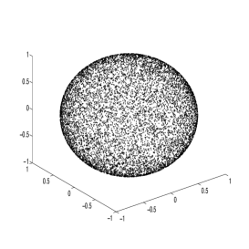
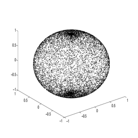
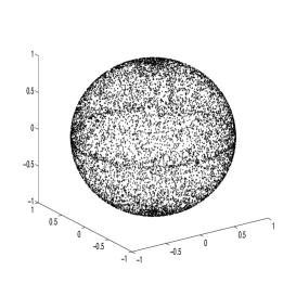
                      (a) (b) (c)                       

Figure 1.1. $m=10,000$ independent draws from the spherical measures (a) $\sin(\theta)\,d\theta d\varphi$, (b) $d\theta d\varphi$, and (c) $|\tan(\theta)|^{1/3}\,d\theta d\varphi$.

1.3. Numerical experiments

In this section we test the numerical relevance of Corollary 1, comparing the rate of correct reconstruction of sparse bandlimited functions on the sphere (1.5) via the $\ell_{1}$-minimizer (1.9) when $m$ sampling points $(\theta_{i},\varphi_{i})$ are drawn i.i.d. from the measures (a) $\sin(\theta)\,d\theta d\varphi$, (b) $d\theta d\varphi$, and (c) $|\tan(\theta)|^{1/3}\,d\theta d\varphi$. More specifically, for each choice of sampling measure, we vary a number of sampling points $m$ between $1$ and $N$, and vary a sparsity level $s$ between $1$ and $m$. For each choice of $m$ and $s$, we generate $50$ $s$-sparse bandlimited functions by repeatedly choosing a support of $[N]$ of size $s$ at random, and prescribing to the chosen support i.i.d. Gaussian coefficients.

From left to right, the phase diagrams in Figure 1.2 correspond to sampling measures (a) $\sin(\theta)d\theta d\varphi$, (b) $d\theta d\varphi$, and (c) $|\tan(\theta)|^{1/3}d\theta d\varphi$. White indicates complete recovery, and black indicates no recovery whatsoever. It is clear that the sampling strategies $(b)$ or $(c)$ give better results than $(a)$. Diagrams (b) and (c) both show a sharp transition between complete recovery and no recovery whatsoever as the ratio $s/m$ increases as a function of $m/N$. However, the region of phase space corresponding to complete recovery is noticeably larger in (3) when $m/N$ is large. Note that when $m=N$, all three sampling schemes should give perfect reconstruction as the system of equations $y=Ac$ in the minimization problem (1.9) has a unique solution with probability $1$. However, plots (a) and (b) show zero reconstruction around this point, an artifact of round-off error due to the ill-conditioning of the sampling matrix $A$.

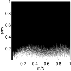
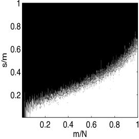
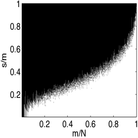
                          (a) (b) (c)                     

Figure 1.2. Phase diagrams illustrating transition between uniform recovery (white) to no recovery whatsoever (black) of spherical harmonic expansions $f(\varphi,\theta)=\sum_{\ell=0}^{19}\sum_{k=-\ell}^{\ell}c_{\ell,k}Y_{\ell}^{k}(\varphi,\theta)$ of sparsity level $|c|\leq s$ from $m$ samples $f(\varphi_{i},\theta_{i})$. In (a), sampling points are drawn from the volume measure $\sin\theta\,d\theta d\varphi$. In (b) the $m$ sampling points are drawn from $d\theta d\varphi$, and in (c) the sampling points are drawn from $|\tan(\theta)|^{1/3}\,d\theta d\varphi$.

Organization of the paper. In Section 2 we review the relationship between sparse recovery techniques on manifolds and weighted $L^{\infty}$ bounds on the associated eigenfunctions. We then show how the main results of this paper strengthen and generalize existing sparse recovery bounds. The generalization of Theorem 1 to arbitrary convex surfaces of revolution is given in Theorem 2 of Section 3, while Section 4 provides a detailed account of preliminaries from semiclassical analysis needed for the proof which is presented in Section 5.

Notation. In the paper $C$ denotes a constant, independent of asymptotic parameters, but changing depending on the context. We use the usual ${\mathcal{O}}$ notation with subscripts to indicate that the associated constant might depend on the variable in the subscript, for instance $f={\mathcal{O}}_{x}(g)$ means that $f(x,y)\leq C(x)g(y)$ for some $C(x)$ depending on $x$. We follow the basic notational convention listed in [12, Appendix A]. Consequently the above notation should not be confused with $u={\mathcal{O}}_{V}(g)$ for $V$ a Hilbert space; the latter means that $\|u\|_{V}\leq Cg$. The notation $f\lesssim g$ means that there exists $C$ such that $f\leq Cg$. Finally, we use the shorthand $[N]=\{1,2,...,N\}$. For a vector $x\in\mathbb{C}^{N}$ or $x\in\mathbb{R}^{N}$, we indicate the size of the support of by $|x|=\{\#j:|x_{j}|>0\}$.

2. Compressed sensing and weighted $L^{\infty}$ estimates

Suppose we have a finite system of functions $\{\psi_{j},j\in[N]\}$ on a compact manifold $M$. Suppose we also have a function $f:{M}\rightarrow\mathbb{C}$ which is $s$-sparse with respect to this function system,

$$f=\sum_{j=1}^{N}c_{j}\psi_{j},\ \ \ \ |c|\leq s<N.$$ (2.1)

The area of compressed sensing [4] is concerned with the following questions. For a given system $\{\psi_{j}\}$ and $s$-sparse function $f$ of the form (2.1), how many samples $f(x_{i})$ where $x_{i}\in M$ do we need to uniquely identify $f$? Is it possible moreover to efficiently and robustly reconstruct such a function from these samples? That is, to distinguish an arbitrary linear combination of $N$ known functions $\psi_{j}$ we would clearly need $N$ samples. But if we know a priori that $f$ is $s$-sparse, and if the locations of the $s$ nonzero coefficients $c_{j}$ are known, then we would need only $s$ samples. When the locations of the $s$ coefficients are not known, $2s$ samples still suffice in certain situations. Namely, consider the matrix $\Psi\in\mathbb{C}^{m\times N}$ with entries $\Psi_{i,j}=\psi_{j}(x_{i})$, and observe that

$$y=\big{(}f(x_{1}),f(x_{2}),\dots,f(x_{m})\big{)}^{t}=\Psi c.$$ (2.2)

Each $s$-sparse function $f$ has a distinct image $y=\Psi c$ if every sub-matrix of the $m\times N$ matrix $\Psi$ consisting of at most $2s$ columns is non-singular, and this is true for many $m\times N$ matrices having only $m=2s$ rows (consider matrices having i.i.d. Gaussian entries, for example.) Subject to this condition, one could solve for the unique $s$-sparse solution to $y=\Psi c$ by searching over all $s$-sparse vectors $c$. However, in general this is an NP-hard problem. As it turns out, polynomial-time recovery of sparse solutions is possible if all $2s$-column sub-matrices of $\Psi$ are not only nonsingular, but well-conditioned - a property that can only hold if $\Psi$ has at least $m\gtrsim s\log(N)$ rows [4]. In the compressed sensing literature, a matrix $\Psi\in\mathbb{C}^{m\times N}$ is said to have the restricted isometry property of order $2s$ if, for a fixed parameter $\delta<1$,

$$(1-\delta)\|u\|_{2}\leq\|\Psi u\|_{2}\leq(1+\delta)\|u\|_{2},\quad\forall u:|u|\leq 2s.$$ (2.3)

As shown in [4], if a matrix $\Psi\in\mathbb{C}^{m\times N}$ has this property, and if $y=\Psi c$ for some $s$-sparse vector $c\in\mathbb{C}^{N}$, then $c$ is guaranteed to also be the vector of minimal $\ell_{1}$-norm among solutions $c^{\prime}$ to the underdetermined system $\Psi c^{\prime}=y$. As $\ell_{1}$-minimization can be solved efficiently using linear programming, the sparse coefficient vector $c$ can be reconstructed efficiently. Moreover, given any arbitrary vector $c\in\mathbb{C}^{N}$ with best $s$-sparse approximation error

$$\varepsilon=\min_{z\in\mathbb{C}^{N}:|z|\leq s}\|c-z\|_{1},$$ (2.4)

and the minimizing solution

$$c^{\sharp}=\arg\min\|z\|_{1}\quad\textrm{subject to }\|\Psi z-\Psi c\|_{2}\leq\epsilon,$$

then $\|c-c^{\sharp}\|_{2}\lesssim\varepsilon/\sqrt{s}$.

2.1. Sparse recovery for bounded orthonormal systems.

In general it is hard to verify the restricted isometry property (2.3) holds for a given matrix $\Psi$, but in the following set-up it can be assured with high probability. Suppose we have a system of functions $\{\psi_{j}$, $j\in[N]\}$ which are orthonormal on a measurable space ${M}$ endowed with a probability measure $\nu$, i.e.

$$\int_{M}\psi_{j}(x)\overline{\psi_{i}(x)}d\nu(x)=\delta_{i,j},\quad i,j\in[N].$$ (2.5)

Suppose further that $m$ sampling points $x_{i}\in M$ are drawn independently from the orthogonalization measure $\nu$. Then, as shown in [21], with high probability with respect to the draw of the sampling points, the normalized sampling matrix $\frac{1}{\sqrt{m}}\Psi$, where $\Psi_{i,j}=\psi_{j}(x_{i})$, satisfies (2.3) as long as the number of samples $m\gtrsim B^{2}s\log^{4}(N)$, where

$$B=\max_{j}\|\psi_{j}\|_{\infty}.$$ (2.6)

The parameter $B$ should be interprested as a measure of incoherence between the basis $\psi_{j}$ and pointwise measurements; the smaller $B$, the fewer number $m$ of sampling points $\big{(}f(x_{1}),f(x_{2}),...,f(x_{m})\big{)}^{t}=\Psi c$ are needed to recover sparse expansions (2.1). This can be interpreted as a discrete Heisenberg uncertainty principle [10]. A precise statement follows.

Proposition 2.1.

Suppose $\{x_{i}:i\in[m]\}$ is a set of independent and identically distributed (i.i.d.) sampling points drawn from the orthogonalization measure $\nu$ associated to an orthonormal system of functions $\{\psi_{j},j\in[N]\}$ with uniform bound $B=\max_{j}\|\psi_{j}\|_{\infty}$. If

$$m\gtrsim B^{2}s\log^{4}(N),$$ (2.7)

then with probability at least $1-N^{-\log^{3}(s)},$ the following holds for all $f(x)=\sum_{j=1}^{N}c_{j}\psi_{j}(x)$ with $s$-term approximation error $\varepsilon$ as in (2.4). Given $m$ observations $y_{i}=f(x_{i})$, or more concisely $y=\Psi c$, and the minimizer

$$c^{\#}=\arg\min_{z\in\mathbb{C}^{N}}\|z\|_{1}\mbox{ subject to }\frac{1}{\sqrt{m}}\|\Psi z-\Psi c\|_{2}\leq\epsilon,$$ (2.8)

it follows that

$$\|c-c^{\#}\|_{2}\lesssim\varepsilon/\sqrt{s}.$$ (2.9)

In particular, if $f$ is $s$-sparse then reconstruction is exact, $c^{\#}=c$.

Let us apply Proposition 2.1 to a concrete example. The orthonormal system of complex exponentials $\psi_{j}(t)=e^{2\pi ijt},t\in[0,1],$ has optimal uniform bound $B=\max_{j}\|\psi_{j}\|_{\infty}=1$. Applying Proposition 2.1, we see that $m\gtrsim s\log^{4}(N)$ sampling points drawn independently from the uniform measure on $[0,1]$ will be sufficient to identify any $s$-sparse trigonometric polynomial of degree at most $N$.

The complex exponentials are eigenfunctions of the Laplacian on the circle. More generally, for a compact $n$-dimensional Riemannian manifold, the $L^{2}$-normalized eigenfunctions with eigenvalue $\lambda$ are bounded in $L^{\infty}$ by $\lambda^{(n-1)/4}$ – see [12, Section 7.4] and references given there. Since the number of eigenvalues less than $\lambda$ behaves like $N=\lambda^{n/2}$ (see [16] or [12, Section 14.3]), we obtain a uniform bound on the first $N$ eigenfunctions of a general $n$-dimensional manifold:

$$B\simeq N^{\frac{n-1}{2n}}.$$

Applying Proposition 2.1 immediately gives the following.

Corollary 2.

Let $(M,g)$ be a compact $n$-dimensional Riemannian manifold and let $\{\psi_{j},j\in[N]\}$ be the first $N$ eigenfunctions of the Laplacian on $M$ (with respect to the ordering of eigenfunctions).

Suppose $\{x_{i}:i\in[m]\}$ is a set of independent and identically distributed sampling points drawn from the measure given by the Riemannian volume. If the number of sampling points satisfies

$$m\gtrsim sN^{\frac{n-1}{n}}\log^{4}(N),$$ (2.10)

then with probability at least $1-N^{-\log^{3}(s)},$ the following holds for all $f(x)=\sum_{j=1}^{N}c_{j}\psi_{j}(x)$.

If $\Psi$ is the sampling matrix associated to the eigenfunctions and sampling points, and if $c^{\#}$ is defined as in (2.8) then

$$\|c-c^{\#}\|_{1}\lesssim\varepsilon,$$

where $\varepsilon$ is the $s$-term approximation error (2.4).

As $n\rightarrow\infty$, the bound (2.10) becomes weaker and weaker. However, even when $n=1$, Proposition 2.1 can be rather restrictive for certain function systems. Consider the ($L^{2}$-normalized) Legendre polynomials $\{P_{j}\}$, the unique orthonormal polynomials with respect to the Lebesgue measure on $[-1,1]$. The Legendre polynomials satisfy $B=\|P_{j}\|_{\infty}=|P_{j}(1)|=(j+1)^{1/2}$. In this situation, Proposition 2.1 gives only that $m\gtrsim sN\log^{4}(N)$ measurements are necessary for identifying functions with an $s$-sparse expansion in the first $N$ Legendre polynomials - a trivial estimate. Proposition 2.1 can however be adapted to give meaningful estimates in a more general setting, as introduced in [23].

Proposition 2.2.

Let $\{\psi_{j},j\in[N]\}$ be an orthonormal system of functions on a probability space ${{M}}$ with orthogonalization measure $\nu$.

Suppose that $\omega:{{M}}\rightarrow\mathbb{R}$ satisfies $\int_{{M}}\omega(x)\nu(x)dx=1$, and suppose that the functions $Q_{j}(x)=\omega(x)^{-1/2}\psi_{j}(x)$ are bounded:

$$\sup_{j\in[N]}\sup_{x\in{M}}|Q_{j}(x)|\leq K.$$ (2.11)

Suppose $\{x_{i}:i\in[m]\}$ are i.i.d. sampling points from the composite orthogonalization measure $\mu=\omega\nu$, and let $A$ be the preconditioned sampling matrix with entries $A_{i,j}=Q_{j}(x_{i})=\omega(x_{i})^{-1/2}\psi_{j}(x_{i})$.

If $m\gtrsim K^{2}s\log^{4}(N)$ then with probability at least $1-N^{-\log^{3}(s)}$ the following holds for all $f(x)=\sum_{j=1}^{N}c_{j}\psi_{j}(x)$ with best $s$-term approximation error $\varepsilon$. Given $m$ observations $y_{k}=f(x_{k})$, or more concisely $y=Ac$, and the minimizer

$$c^{\#}=\arg\min_{z\in\mathbb{C}^{N}}\|z\|_{1}\mbox{ subject to }\frac{1}{\sqrt{m}}\|Az-Ac\|_{2}\leq\epsilon,$$ (2.12)

it follows that

$$\|c-c^{\#}\|_{2}\lesssim\varepsilon/\sqrt{s}.$$ (2.13)

Proof.

Apply Proposition 2.1 to the system $\{Q_{j}\}_{j\in[N]}$, which is a bounded orthonormal system: $\sup_{j\in[N]}\|Q_{j}\|_{\infty}\leq K$ and the $Q_{j}$ are orthonormal with respect to the composite measure $\mu=\omega\nu$. ∎

Proposition 2.2 quantifies the link between weighted $L^{\infty}$ estimates on orthonormal function systems and sparse recovery guarantees. For the Legendre polynomials, which satisfy the weighted $L^{\infty}$ estimate

$$(1-x^{2})^{1/2}|P_{j}(x)|\leq 2\sqrt{\pi},$$

Proposition 2.2 gives that $m\gtrsim s\log^{4}{N}$ sampling points from the Chebyshev measure $\mu(x)=\sin^{-1/2}(x)dx$ are sufficient for recovering $s$-sparse expansions in the first $N$ Legendre polynomials. For details, see [23].

Below we summarize how the weighted $L^{\infty}$ estimates of this paper improve and generalize previous results and give rise to Proposition 1.1.

1. In [19], Krasikov proves the following weighted $L^{\infty}$ estimate for the spherical harmonics $Y_{\ell}^{k}$:

   $$(\sin\theta)^{1/2}|Y_{\ell}^{k}(\varphi,\theta)|\lesssim\ell^{1/4}.$$

   This estimate implies

   $$\sup_{0\leq\ell\leq\sqrt{N}-1}\sup_{-\ell\leq k\leq\ell}(\sin\theta)^{1/2}|Y_{\ell}^{k}(\varphi,\theta)|\lesssim N^{1/8}.$$ (2.14)

   In [24], the authors apply Proposition 2.2 using this estimate to conclude that $m\gtrsim sN^{1/4}\log^{4}N$ sampling points on the sphere with angular coordinates $(\theta_{i},\varphi_{i})$ drawn independently from the measure $d\theta d\varphi$ on $[0,\pi]\times[0,2\pi)$ suffice for recovering bandlimited sparse spherical harmonic expansions of the form (1.5). This improved on the $m\gtrsim sN^{1/2}\log^{4}(N)$ required sampling points given by Corollary 2, if sampling points are drawn i.i.d. from the uniform distribution on the sphere.

2. The weighted $L^{\infty}$ estimate given in Theorem 1 provides even stronger sparse recovery guarantees for spherical harmonic expansions. Corollary 1 results from applying this estimate to Proposition 2.2: $m\gtrsim sN^{1/6}\log^{4}(N)$ sampling points $(\theta_{i},\varphi_{i})$ from the measure $|\tan(\theta)|^{1/3}d\theta d\varphi$ suffice for recovering sparse bandlimited spherical harmonic expansions (1.5).

3. As summarized in Proposition 1.1, the weighted $L^{\infty}$ estimate of Corollary 3 gives rise to more general sampling strategies for recovering sparse eigenfunction expansions on strictly convex surfaces of revolution.

3. Weighted eigenfunction estimates for surfaces of revolution

If $M$ be a smooth surface of revolution, let $\partial_{\varphi}$ be the vector field generating the action of the circle $\mathbb{S}^{1}=\mathbb{R}/(2\pi\mathbb{Z})$ on $M$ by rotations around the axis of revolution. Denote by $\Delta$ the Laplace–Beltrami operator on $M$, and by $D_{\varphi}$ the self-adjoint operator $\frac{1}{i}\partial_{\varphi}$ which commutes with $\Delta$. This follows the standard convention for the operators quantizing momenta.

Let $h>0$ be a small parameter, and assume that $u\in{\mathcal{C}}^{\infty}(M)$ satisfies the conditions

$$\|u\|_{L^{2}}\leq C_{0}\,,$$ (3.1)

$$\|(-h^{2}\Delta-1)u\|_{L^{2}}\leq C_{0}h\,,$$ (3.2)

$$(hD_{\varphi}-\alpha)u=0\,.$$ (3.3)

Here $\alpha\in h\mathbb{Z}$ varies in a fixed compact set and $C_{0}$ is some fixed constant. Both $-h^{2}\Delta-1$ and $hD_{\varphi}-\alpha$ are semiclassical differential operators; we will freely use the notation of semiclassical analysis that can be found, for example, in [12, Chapter 4].

We also assume that $u$ satisfies the following localization assumption: there exists a compactly microlocalized operator $X(h)$ (that is, $X(h)=\psi^{w}(x,hD_{x})+\mathcal{O}_{H^{-N}_{h}\to H^{N}_{h}}(h^{N})$ for some $\psi\in{\mathcal{C}}^{\infty}_{\rm{c}}(T^{*}M)$ and each $N$) and fixed constants $C_{N}$ such that for each $N$,

$$\|(1-X(h))u\|_{H^{N}_{h}}\leq C_{N}h^{N}.$$ (3.4)

Remark: Conditions (3.1), (3.2), and (3.4) are in particular satisfied if $u$ is an $L^{2}$ normalized eigenfunction of $-\Delta$ for an eigenvalue in the segment

$$h^{-2}[1-C_{0}h,1+C_{0}h]\,,$$

as applied in Proposition 1.1.

The weaker condition (3.2) has the advantage that it is local:

Figure 3.1. A surface of revolution

Proposition 3.1.

Assume that $\chi\in{\mathcal{C}}^{\infty}(M)$ and $D_{\varphi}\chi=0$. If $u$ satisfies (3.1)–(3.3), then $\chi u$ satisfies these conditions as well, possibly with larger value of the constant $C_{0}$.

Similarly, if condition (3.4) holds for $u$, it holds for $\chi u$.

Proof.

Conditions (3.1) and (3.3) for $\chi u$ are trivially satisfied; we now verify (3.2). Since the commutator $[-h^{2}\Delta,\chi]$ is equal to $h$ times a semiclassical differential operator of order 1, we have

$$\begin{gathered}\|(-h^{2}\Delta-1)\chi u\|_{L^{2}}\leq\|\chi(-h^{2}\Delta-1)u\|_{L^{2}}+\|[-h^{2}\Delta,\chi]u\|_{L^{2}}\\ =\mathcal{O}(h(1+\|u\|_{H^{1}_{h}})).\end{gathered}$$

However,

$$\|u\|_{H^{1}_{h}}^{2}\sim((-h^{2}\Delta+1)u,u)_{L^{2}}={\mathcal{O}}(1)$$

by (3.1) and (3.2). Here $H_{h}^{s}$ denotes the semiclassical Sobolev space defined using the norm $\|(I-h^{2}\Delta_{M})^{s/2}u\|_{L^{2}}$.

To verify (3.4), we use that $\chi u=\chi X(h)u+{\mathcal{O}}_{{\mathcal{C}}^{\infty}}(h^{\infty})$; however, if $Y(h)$ is a compactly microlocalized pseudodifferential operator equal to the identity microlocally near the wavefront set of $X(h)$ (and thus of $\chi X(h)$), then $(1-Y(h))\chi u=(1-Y(h))\chi X(h)u+{\mathcal{O}}_{{\mathcal{C}}^{\infty}}(h^{\infty})={\mathcal{O}}_{{\mathcal{C}}^{\infty}}(h^{\infty})$.

∎

Proposition 3.1 implies that, if we want to obtain weighted $L^{\infty}$ (or any other local) estimates on every function $u$ satisfying (3.1)–(3.3), it is enough to cover $M$ by open sets invariant under rotation (which we will call bands) and prove the estimates for functions supported in each of these bands. The next result provides weighted $L^{\infty}$ estimates for three common types of behavior of the metric in bands:

Theorem 2.

Let $U_{\varepsilon}\subset M$ be a band given by one of the three cases below; the small parameter $\varepsilon>0$ characterizes the width of this band. Then for $\varepsilon>0$ and $h>0$ small enough and some constant $C$, and for each $\alpha\in h\mathbb{Z}$ varying in a fixed compact set, each function $u\in{\mathcal{C}}^{\infty}(M)$ supported in $U_{\varepsilon}$ and satisfying (3.1)–(3.4) has the following weighted $L^{\infty}$ estimates:

Figure 3.2. Three considered types of bands, with a geodesic shown for each type

1. Regular case: $U_{\varepsilon}$ has coordinates $(r,\varphi)\in(-\varepsilon,\varepsilon)\times\mathbb{S}^{1}$ and the metric

   $$g=g(r)[dr^{2}+d\varphi^{2}].$$ (3.5)

   Here $g$ is a smooth function independent of $\varepsilon$, and $g(0)>0$, $g^{\prime}(0)\neq 0$. The corresponding estimate is

   $$|u(r,\varphi)|\leq Ch^{-1/6}.$$ (3.6)

2. Elliptic equator: $U_{\varepsilon}$ has the same coordinates and metric as in the regular case, but $g(0)>0$, $g^{\prime}(0)=0$, and $g^{\prime\prime}(0)<0$. The corresponding estimates are

   $$|u(r,\varphi)|\leq C\min(h^{-1/4}\,,\,h^{-1/6}r^{-1/6}\,,\,h^{-1/6}|g(0)-\alpha^{2}|^{-1/12});$$ (3.7)

   $$|u(r,\varphi)|\leq Cr^{-1/2}\ \text{ for }|g(0)-\alpha^{2}|<\varepsilon r^{2}.$$ (3.8)

3. Pole: $U_{\varepsilon}$ has coordinates $(x,y)=(r\cos\varphi,r\sin\varphi)$, with $|x|^{2}+|y|^{2}<\varepsilon^{2}$, and the metric

   $$g=g(x^{2}+y^{2})[dx^{2}+dy^{2}]=g(r^{2})[dr^{2}+r^{2}\,d\varphi^{2}],$$ (3.9)

   where $g$ is a smooth function and $g(0)>0$. The corresponding estimates are

   $$|u(r,\varphi)|\leq C\min(h^{-1/2}\,,\,h^{-1/6}r^{-1/3}\,,\,h^{-1/6}|\alpha|^{-1/3});$$ (3.10)

   $$|u(r,\varphi)|\leq Cr^{-1/2}\ \text{ for }|\alpha|<\varepsilon r.$$ (3.11)

Remark. The metric of a surface of revolution can be brought locally to the form (3.5) or (3.9), with $g(0)>0$, with no conditions on the derivatives of $g$. Indeed, away from the poles (points on the surface lying on the axis of rotation), the metric has the form

$$(1+\tilde{g}^{\prime}(\tilde{r})^{2})d\tilde{r}^{2}+\tilde{g}(\tilde{r})^{2}\,d\varphi^{2},$$

where $\tilde{r}$ is the projection onto the axis of rotation and $\tilde{g}$ is a positive function giving the profile of the surface. Making a change of variables $\tilde{r}\to r$ with $dr/d\tilde{r}=\tilde{g}(\tilde{r})^{-1}\sqrt{1+\tilde{g}^{\prime}(\tilde{r})^{2}}$, we bring the metric to the form (3.5). The case of a pole is handled similarly. As $(\tilde{r},\varphi)$ we can use the geodesic polar coordinates with respect to the pole and a different change of variables $\tilde{r}\to r$.

We obtain the following corollary for convex surfaces of revolution. The estimate is the analogue of the estimate (1.4) in the case of the sphere:

Corollary 3.

Suppose that $M$ is a strictly convex surface of revolution parametrized by $(r,\varphi)\in[r_{-},r_{+}]\times[0,2\pi)$, with the metric $dr^{2}+a(r)\,d\varphi^{2}$ as in the discussion preceeding Proposition 1.1. Suppose that

$$(\Delta-\lambda)u=0,\ \ (\textstyle{\frac{1}{i}}\partial_{\varphi}-k)u=0,\ \|u\|_{L^{2}(M)}=1.$$ (3.12)

Then,

$$a(r)^{1/3}|r-r_{0}|^{1/6}|u(r,\varphi)|\leq C\lambda^{1/12}.$$ (3.13)

The Riemannian volume measure on $M$ is given by $a(r)drd\varphi$ which means that the sampling measure based on (3.13) should be given by

$$\left(\frac{a(r)}{|r-r_{0}|}\right)^{1/3}drd\theta;$$

here $a(r)/(r-r_{0})$ is the replacement for $\tan\theta$. The constant $K$ in (2.11) is given by

$$K\simeq N^{1/12}.$$

Theorem 2 does not cover the case of a band with metric of the form (3.5) and $g^{\prime}(0)=0$, $g^{\prime\prime}(0)\leq 0$; in particular, it does not apply to the case of a hyperbolic equator, when $g^{\prime\prime}(0)<0$. This case does not occur for convex surfaces considered here.

Let us give an informal explanation of the estimates in Theorem 2. By considering an eigenfunction decomposition of $u$, we can reduce to the case when $u$ is an exact joint eigenfunction of $-h^{2}\Delta$ and $hD_{\varphi}$, rather than a function satisfying (3.2). Using semiclassical analysis (see [12] for the general theory and the references below for specific facts we will be using), we can relate the behavior of the ‘quantum’ object $u$ for small values of the ‘Planck constant’ $h$ to the corresponding ‘classical’ integrable Hamiltonian system given by the principal symbols $p$ and $q$ of $-h^{2}\Delta$ and $hD_{\varphi}$, respectively. The principal symbol of a differential operator is a polynomial (on each fiber) function on the cotangent bundle $T^{*}M$, obtained formally by replacing each instance of $hD_{x_{j}}$ by the corresponding momentum $\xi_{j}$, and then discarding the terms of higher order in $h$. In our situation, $p$ is the square of the norm induced by $g$ on the cotangent bundle and $q$ is the momentum corresponding to $\varphi$. The function $u$ will then be concentrated, or microlocalized, on the set

$$\Lambda=\{p=1,\ q=\alpha\}\subset T^{*}M.$$

One can in fact approximate $u$ by certain explicit highly oscillating integral expressions up to an $\mathcal{O}(h^{\infty})$ error; our analysis would consist of studying the asymptotic behavior of these integrals as $h\to 0$. The set $\Lambda$ consists of unit geodesics with prescribed angular momentum (that is, of rotations of one such geodesic); there are two possibilities:

1. $\Lambda$ is a Lagrangian torus;

2. $\Lambda$ is a circle corresponding to an equator.

In case (1), $u$ is a Lagrangian distribution associated to $\Lambda$ – that is, it can be written as a finite sum of expressions of the WKB form (4.1), with $\Phi(x,\theta)$ locally parametrizing the Lagrangian $\Lambda$ and $a$ some smooth symbol – see Section 4.1 for details. The $L^{\infty}$ norm of $u$ corresponds to how well $\Lambda$ projects onto the base space $M$. At a point where the tangent space of $\Lambda$ projects surjectively onto $M$, the $L^{\infty}$ norm of $u$ is $\mathcal{O}(1)$. The only other possibility that could arise in the regular case is a turning point; that is, a point where the function $r$ has a nondegenerate critical point when restricted to a geodesic (for the sphere, these are the points of maximal and minimal latitude on a given great circle). The behavior of $u$ near the turning points is similar to that of the Airy function, and its $L^{\infty}$ norm is of order $h^{-1/6}$ by a variant of Van der Corput’s lemma.

If one is unfamiliar with Lagrangian distributions, the simple model case to consider would be the eigenfunctions of the Laplacian $h^{2}D_{x}^{2}$ on the circle $\mathbb{S}^{1}=\mathbb{R}/(2\pi\mathbb{Z})$. Those are given by $e^{i\lambda x/h}$, with the eigenvalue $\lambda^{2}$. (Note that only a discrete set of $\lambda$ is possible here – this is a baby version of the quantization condition mentioned in the next section.) The corresponding symbol is $p(x,\xi)=\xi^{2}$ and the corresponding Lagrangian would be $\{x\in\mathbb{S}^{1},\ \xi=\lambda\}$; it projects surjectively onto the $x$ variables, which corresponds to the fact that we do not need any integration variables $\theta$ in the formula (4.1) to define eigenfunctions, and to the fact that the $L^{\infty}$ norm of eigenfunctions is bounded by a constant.

For $\alpha=0$, a new kind of problem arises – the intersection of $\Lambda$ with the fiber of $T^{*}M$ at a pole is a not a point, but a circle consisting of all unit covectors at the pole, leading to a loss of $h^{-1/2}$ in the $L^{\infty}$ norm. This problem disappears and we get back the $h^{1/6}$ estimate if either $\alpha$ is away from zero or we are away from the pole, which is reflected in (3.10). If $\alpha=0$, the turning points are located at the poles; therefore, away from the poles we get an $\mathcal{O}(1)$ estimate. The blow-up rate of this estimate as we approach a pole is quantified by (3.11).

In case (2) we can separate out the $\varphi$ variable (as $\Lambda$ does not pass through any poles) and obtain a one-dimensional problem; then $u$ is a low-lying eigenfunction of a Schrödinger operator with a potential well. The bottom of the well eigenfunctions (those with $g(0)-\alpha^{2}=\mathcal{O}(h)$) are approximated by the Gaussian $h^{-1/4}e^{-r^{2}/(2h)}$; we see that they are

$$\mathcal{O}(\min(h^{-1/4},r^{-1/2}))\,.$$

This explains the first part of (3.7) and (3.8). However, if $g(0)-\alpha^{2}$ is bounded away from zero, we are away from the equator and thus back to case (1), which explains the $h^{-1/6}$ term in (3.7).

4. Preliminaries

4.1. Semiclassical Lagrangian distributions

In this subsection, we briefly review the local theory of semiclassical Lagrangian distributions; see for example [2],[14, Chapter 6], [15, Chapter 8] or [27, Section 2.3] for a detailed account, and [18, Section 25.1] or [13, Chapter 11] for the presentation in the closely related microlocal case.

Assume that $X$ is a manifold and $\Phi(x,\theta)$ is a smooth real-valued function defined on an open set $U_{\Phi}\subset X\times\mathbb{R}^{m}$. Define the critical set $C_{\Phi}\subset U_{\Phi}$ by

$$(x,\theta)\in C_{\Phi}\iff\partial_{\theta}\Phi(x,\theta)=0.$$

The function $\Phi$ is called a (nondegenerate) phase function, if for each $(x,\theta)\in C_{\Phi}$, the differentials $d(\partial_{\theta_{1}}\Phi),\dots,d(\partial_{\theta_{m}}\Phi)$ are linearly independent at $(x,\theta)$. If this is the case, the set

$$\Lambda_{\Phi}=\{(x,\partial_{x}\Phi(x,\theta))\mid(x,\theta)\in C_{\Phi}\}\subset T^{*}X$$

is an (immersed) Lagrangian submanifold. We say that $\Phi$ generates $\Lambda_{\Phi}$; in general, if $\Lambda\subset T^{*}X$ is a Lagrangian submanifold and $(x,\xi)\in\Lambda_{\Phi}\subset\Lambda$, then we say that $\Phi$ generates $\Lambda$ near $(x,\xi)$. For each Lagrangian submanifold $\Lambda$ and each $(x,\xi)\in\Lambda$, there exists a phase function generating $\Lambda$ near $(x,\xi)$; however, such phase function is not unique.

If $\Lambda\subset T^{*}X$ is an (embedded) Lagrangian submanifold, $\Phi$ is a phase function generating $\Lambda$ near some point, and $a(x,\theta;h)\in{\mathcal{C}}^{\infty}_{\rm{c}}(U_{\Phi})$ is bounded in ${\mathcal{C}}^{\infty}_{x,\theta}$ uniformly in $h$, we can define the $h$-dependent family of smooth functions

$$u(x;h)=h^{-m/2}\int e^{i\Phi(x,\theta)/h}a(x,\theta)\,d\theta.$$ (4.1)

Here the factor $h^{-m/2}$ is chosen so that $\|u(x;h)\|_{L^{2}}$ is bounded by a certain ${\mathcal{C}}^{\infty}$ seminorm of $a$ and equivalent to the $L^{2}$ norm of $a|_{C_{\Phi}}$, modulo ${\mathcal{O}}(h)$ terms. We call $u(x;h)$ a (semiclassical compactly microlocalized) Lagrangian distribution associated to $\Lambda$. This family is microlocalized on $\Lambda_{\Phi}$ in the following sense:

$$b\in{\mathcal{C}}^{\infty}_{\rm{c}}(T^{*}X)\,,\ b|_{\operatorname{neigh}(\Lambda_{\Phi})}=0\ \Longrightarrow\ \|b^{w}(x,hD_{x})u(x;h)\|_{L^{2}}={\mathcal{O}}(h^{\infty})\,.$$

More generally, we call $u(x;h)$ a Lagrangian distribution associated to $\Lambda$, if it is the sum of finitely many expressions of the form (4.1), for different phase functions parametrizing $\Lambda$, and an ${\mathcal{O}}_{{\mathcal{C}}^{\infty}_{\rm{c}}}(h^{\infty})$ remainder.

If $u(x;h)$ is a Lagrangian distribution associated to $\Lambda$, $\Phi$ is a phase function generating $\Lambda$, and $u$ is microlocalized in a compact subset of $\Lambda_{\Phi}$, then we can always write $u$ in the form (4.1) for some amplitude $a$ modulo an ${\mathcal{O}}(h^{\infty})$ remainder. (The general case can always be reduced to this one by a microlocal partition of unity, if we know enough phase functions to cover the whole $\Lambda$.) In other words, if two phase functions locally generate the same Lagrangian, then oscillatory integrals (4.1) associated to one phase function can be written in the form (4.1) using the other phase function as well. However, the formulas relating even the principal parts of the amplitudes corresponding to different phase functions are quite complicated; obtaining a geometric interpretation for these formulas is the subject of global theory of Lagrangian distributions. This global theory is needed to produce quantization conditions that we use below; however, as we are only interested in estimating the resulting eigenfunctions and in some rough properties of the spectrum given by quantization conditions, we do not use the global theory directly.

4.2. Specific generating functions and $L^{\infty}$ estimates

In this subsection, we assume that $\Lambda\subset T^{*}\mathbb{R}^{n}$ is a Lagrangian submanifold and $(x^{0},\xi^{0})\in\Lambda$.

Proposition 4.1.

Take $0\leq m\leq n$ and denote $x=(x^{\prime},x^{\prime\prime}),\xi=(\xi^{\prime},\xi^{\prime\prime})$, where $x^{\prime},\xi^{\prime}\in\mathbb{R}^{m}$ and $x^{\prime\prime},\xi^{\prime\prime}\in\mathbb{R}^{n-m}$. Assume that $T_{(x^{0},\xi^{0})}\Lambda$ projects surjectively onto the $(x^{\prime},\xi^{\prime\prime})$ variables. Then there exists a function $S(x^{\prime},\xi^{\prime\prime})$ such that near $(x^{0},\xi^{0})$, $\Lambda$ is given by

$$\{\xi^{\prime}=-\partial_{x^{\prime}}S(x^{\prime},\xi^{\prime\prime}),\ x^{\prime\prime}=\partial_{\xi^{\prime\prime}}S(x^{\prime},\xi^{\prime\prime})\}.$$

Consequently, $\Lambda$ is generated near $(x^{0},\xi^{0})$ by the phase function

$$\Phi(x,\theta)=x^{\prime\prime}\cdot\theta-S(x^{\prime},\theta),\ \theta\in\mathbb{R}^{n-m}.$$

Proof.

For the reader’s convenience we recall the well known argument. We can write $\Lambda$ locally as a graph $\{\xi^{\prime}=-F(x^{\prime},\xi^{\prime\prime}),\ x^{\prime\prime}=G(x^{\prime},\xi^{\prime\prime})\}$. The restriction of the symplectic form $d\xi\wedge dx$ to $\Lambda$ is zero; therefore, the restriction of the 1-form $\alpha=x^{\prime\prime}\,d\xi^{\prime\prime}-\xi^{\prime}\,dx^{\prime}$ to $\Lambda$ is closed. Therefore, there exists a function $S(x^{\prime},\xi^{\prime\prime})$ such that $\alpha=dS$ when restricted to $\Lambda$. However, if we use $(x^{\prime},\xi^{\prime\prime})$ as a coordinate system on $\Lambda$, then $\alpha=G\,d\xi^{\prime\prime}+F\,dx^{\prime}$ and $dS=\partial_{\xi^{\prime\prime}}S\,d\xi^{\prime\prime}+\partial_{x^{\prime}}S\,dx^{\prime}$; it follows that $F=\partial_{x^{\prime}}S$ and $G=\partial_{\xi^{\prime\prime}}S$. ∎

In one special case $\Lambda$ can be locally parametrized by $x$; the corresponding Lagrangian distributions satisfy the best $L^{\infty}$ estimate possible:

Proposition 4.2.

Assume that the tangent space to $\Lambda$ at each point projects surjectively onto the $x$ variables. Then, each Lagrangian distribution $u(x;h)$ associated to $\Lambda$ satisfies $\|u(x;h)\|_{L^{\infty}}={\mathcal{O}}(1)$.

Proof.

Putting $x^{\prime}=x$ and $x^{\prime\prime}=\emptyset$ in Proposition 4.1, we get a phase function $\Phi(x)=-S(x)$. The expression (4.1) for this phase function has the form $e^{-iS(x)/h}a(x;h)$ and is trivially ${\mathcal{O}}(1)$ in $L^{\infty}$. ∎

If $\Lambda$ does not satisfy the condition of Proposition 4.2, then the associated Lagrangian distributions can have $L^{\infty}$ norm as large as $h^{-n/2}$. However, in some cases we are still able to find a phase function satisfying some additional conditions that will ensure a better bound. We will in particular use the following estimate for the case when $\theta$ is one-dimensional:

Proposition 4.3.

Assume that $\Phi(x,\theta)$, $(x,\theta)\in U\subset\mathbb{R}^{n}\times\mathbb{R}$, is a phase function and

$$|\partial_{\theta}\Phi(x,\theta)|+|\partial_{\theta}^{2}\Phi(x,\theta)|+|\partial_{\theta}^{3}\Phi(x,\theta)|>0\text{ for each }(x,\theta)\in U.$$

Then each oscillatory integral $u(x;h)$ of the form (4.1) satisfies

$$\|u\|_{L^{\infty}}={\mathcal{O}}(h^{-1/6}).$$

Proof.

This follows from the van der Corput’s Lemma as presented in [26, Proposition VIII.2]. We can also argue using more precise asymptotics which are relevant when precise information at the caustic is needed: If the amplitude $a(x,\theta;h)$ is supported in a region where $|\partial_{\theta}\Phi|+|\partial_{\theta}^{2}\Phi|>0$, then we can apply the stationary phase method to (4.1) to get $\|u\|_{L^{\infty}}={\mathcal{O}}(1)$. (Alternatively, the corresponding piece of the Lagrangian $\Lambda_{\Phi}$ will satisfy the condition of Proposition 4.2.) If at $(x_{0},\theta_{0})$ we have $\partial_{\theta}\Phi(x_{0},\theta_{0})=\partial^{2}_{\theta}\Phi(x_{0},\theta_{0})=0$ and $\partial^{3}_{\theta}\Phi(x_{0},\theta_{0})\neq 0$, then we can apply [17, Theorem 7.7.18] which shows that for $a$ supported near $(x_{0},\theta_{0})$, there exist smooth functions $a_{1},a_{2},b$ such that $a_{1},b$ are real-valued and

$$h^{-\frac{1}{2}}\int e^{i\Phi(x,\theta)/h}a(x,\theta)\,d\theta=h^{-1/6}e^{ib(x)/h}Ai(h^{-\frac{2}{3}}a_{1}(x))a_{2}(x)+{\mathcal{O}}(h^{\frac{1}{6}})\,.$$

Since the Airy function $Ai$ is bounded, this expression is $\mathcal{O}(h^{-1/6})$. A partition of unity argument finishes the proof of the proposition. ∎

4.3. $L^{\infty}$ estimates for potential wells

Assume that $V(x)$, $x\in\mathbb{R}$, is a smooth real-valued potential such that:

• for each $N$, there exists a constant $C_{N}$ such that $|\partial_{x}^{N}V(x)|\leq C_{N}(1+|x|^{2})$ for all $x$;

• there exists a constant $\varepsilon_{V}>0$ such that $V(x)\geq\varepsilon_{V}|x|^{2}$ for all $x$;

• $V(0)=V^{\prime}(0)=0$, $V^{\prime\prime}(0)=2c^{2}$ for some $c>0$, and $\pm V^{\prime}(x)>0$ for $\pm x>0$.

Consider the semiclassical Schrödinger operator

$$P(h)=h^{2}D_{x}^{2}+V(x);$$

let $p(x,\xi)=\xi^{2}+V(x)$ be the corresponding principal symbol. Since $p(x,\xi)\to\infty$ as $|x|+|\xi|\to\infty$, it follows [12, Section 6.3] that $P(h)$ is a self-adjoint operator on $L^{2}(\mathbb{R})$ with compact resolvent and therefore posesses a complete orthonormal system of eigenfunctions.

For $\lambda>0$, $p$ does not have critical points on $p^{-1}(\lambda)$ and thus produces a completely integrable one-dimensional Hamiltonian system. The following is a corollary of the spectral theory of self-adjoint operators corresponding to quantum completely integrable systems (see [14, Section 2.7] or [27, Theorème 5.1.11]):

Proposition 4.4.

Let $K$ be a compact subset of $(0,\infty)$. Then for $h$ small enough, the eigenvalues $\lambda$ of $P(h)$ in $K$ are simple and given by the quantization condition

$$S(\lambda)=(2j+1)\pi h+{\mathcal{O}}(h^{2}),\ j\in\mathbb{Z},\$$ (4.2)

where $S(\lambda)$ is the action functional:

$$S(\lambda)=\oint_{p(x,\xi)=\lambda}\xi\,dx$$

and the curve $p^{-1}(\lambda)$ is oriented clockwise. In particular, $S$ is smooth and $S^{\prime}(\lambda)>0$ everywhere. Moreover, each $L^{2}$ normalized joint eigenfunction corresponding to an eigenvalue $\lambda\in K$ is a Lagrangian distribution associated to $p^{-1}(\lambda)$ (that is, it admits a parametrization by integrals of the form (4.1) with estimates on the symbol and the remainder uniform in $\lambda$).

Remark. The quantization condition (4.2) is valid for the eigenvalues close to zero as well, if we add the requirement that $j\geq 0$. This can be proved by conjugating $P(h)$ by a semiclassical Fourier integral operator to a function of the harmonic oscillator; it follows from the analysis in [6] and can be found for example in [27, Theorème 5.2.4].

For $\lambda$ away from zero, we get the following estimate on eigenfunctions of $P(h)$:

Proposition 4.5.

Let $K$ be a compact subset of $(0,\infty)$. Then each $L^{2}$-normalized eigenfunction $v_{\lambda}$ with eigenvalue $\lambda\in K$ satisfies

$$\|v_{\lambda}\|_{L^{\infty}}={\mathcal{O}}(h^{-1/6}).$$

Proof.

Figure 4.1. The curve $p^{-1}(\lambda)$ and the regions $\Gamma_{\pm}$

By Proposition 4.4, $v_{\lambda}$ is a Lagrangian distribution associated to the curve $p^{-1}(\lambda)$. Let $\Gamma_{\pm}$ be the intersections of $p^{-1}(\lambda)$ with small neighborhoods of the turning points $(x_{\pm}(\lambda),0)$; here $x_{-}(\lambda)<x_{+}(\lambda)$ are the two roots of the equation $V(x)=\lambda$. Away from $\Gamma_{\pm}$, the curve $p^{-1}(\lambda)$ projects diffeomorphically onto the $x$ axis; therefore, by Proposition 4.2, Lagrangian distributions associated to $p^{-1}(\lambda)\setminus(\Gamma_{+}\cup\Gamma_{-})$ have $L^{\infty}$ norm ${\mathcal{O}}(1)$. It remains to consider the case of a Lagrangian distribution associated to, say, $\Gamma_{+}$. However, $\Gamma_{+}$ can be parametrized by $\xi$ and thus by Proposition 4.1 it has a generating function of the form $\Phi(x,\xi)=x\xi-T(\xi)$. We can calculate that $\partial_{\xi}^{3}T(\xi)$ is nonvanishing; it remains to apply Proposition 4.3. ∎

Using Proposition 4.5 together with elliptic estimates, we get $L^{\infty}$ bounds on functions satisfying the analogue of (3.2):

Proposition 4.6.

Assume $\lambda\in\mathbb{R}$ lies in a fixed compact set $K$ and $u\in\mathcal{{\mathcal{C}}^{\infty}_{\rm{c}}}(\mathbb{R})$ satisfies

$$\|u\|_{L^{2}}\leq C_{0},\ \|(P(h)-\lambda)u\|_{L^{2}}\leq C_{0}h,$$ (4.3)

for some constant $C_{0}$. Then:

1. If $\chi\in{\mathcal{C}}^{\infty}_{\rm{c}}(T^{*}\mathbb{R})$ is equal to 1 near $p^{-1}(\lambda)$, then

   $$\|(1-\chi^{w}(x,hD_{x}))u\|_{L^{\infty}}=\mathcal{O}_{\chi,\lambda}(1).$$

   In particular, if $\pi:T^{*}\mathbb{R}\to\mathbb{R}$ is the projection map, then

   $$x\not\in\pi(p^{-1}(\lambda))\Longrightarrow\ |u(x)|=\mathcal{O}_{x,\lambda}(1)\,.$$ (4.4)

   The constants in $\mathcal{O}(\cdot)$ are locally uniform in $x,\lambda$.

2. If $|\lambda|\geq\delta$ for some constant $\delta>0$, then

   $$\|u\|_{L^{\infty}}={\mathcal{O}}_{\delta}(h^{-1/6}).$$

3. If $|x|\geq\delta$ for some constant $\delta>0$, then

   $$|u(x)|={\mathcal{O}}_{\delta}(h^{-1/6}).$$

Remark. We do not assume the localization condition (3.4) and work only under the hypothesis (4.3). That is because we will apply the proposition to a rescaled version of the original $u$ which no longer satisfies (3.4).

Proof.

1. The operator $P(h)-\lambda$ is elliptic with respect to the order function $m(x,\xi)=1+x^{2}+\xi^{2}$ on $\operatorname{supp}(1-\chi)$; therefore, the elliptic parametrix construction (as in [12, Section 4.5] or [7, Proposition 8.6], with minor adjustments found for example in [11, Proposition 5.1]) gives a symbol $q\in S(m^{-1})$ such that

$$q^{w}(x,hD_{x})(P(h)-\lambda)=1-\chi^{w}(x,hD_{x})+{\mathcal{O}}_{L^{2}\to L^{2}}(h^{\infty}).$$

Therefore, by Sobolev embedding

$$\begin{split}\|(1-\chi^{w}(x,hD_{x}))u\|_{L^{\infty}}&\lesssim\|(1-\chi^{w}(x,hD_{x}))u\|_{H^{1}}\lesssim h^{-1}\|(1-\chi^{w}(x,hD_{x}))u\|_{H^{1}_{h}}\\ &\lesssim h^{-1}\|q^{w}(x,hD_{x})(P(h)-\lambda)u\|_{H^{1}_{h}}+{\mathcal{O}}(h^{\infty})\|u\|_{L^{2}}\\ &\lesssim h^{-1}\|(P(h)-\lambda)u\|_{L^{2}}+{\mathcal{O}}(h^{\infty})\|u\|_{L^{2}}={\mathcal{O}}(1).\end{split}$$

To show (4.4), it suffices to apply the previous inequality with $\chi$ vanishing near $\pi^{-1}(x)$, but equal to 1 near $p^{-1}(\lambda)$.

2. If $\lambda\leq-\delta$, then $p^{-1}(\lambda)=\emptyset$ and thus part 1 of this proposition applies with $\chi\equiv 0$. We now assume that $\lambda\geq\delta$. Take $\tilde{\chi}\in{\mathcal{C}}^{\infty}_{\rm{c}}(\lambda/2,2\lambda)$ equal to 1 near $\lambda$; then the operator $\tilde{\chi}(P(h))$, defined by means of functional calculus, is pseudodifferential, compactly microlocalized, and equal to the identity microlocally near $p^{-1}(\lambda)$ [7, Chapter 8]. By part 1 of this proposition, we have

$$u=\tilde{\chi}(P(h))u+{\mathcal{O}}_{L^{\infty}}(1);$$

it remains to estimate $\|\tilde{\chi}(P(h))u\|_{L^{\infty}}$. Let $v_{1},v_{2},\ldots\in{\mathcal{C}}^{\infty}$ be the orthonormal basis of $L^{2}(\mathbb{R})$ consisting of eigenfunctions of $P(h)$ with eigenvalues $\lambda_{1},\lambda_{2},\dots$. If

$$u=\sum_{j}c_{j}v_{j},$$

then by (4.3),

$$\begin{gathered}\sum_{j}(|\lambda_{j}-\lambda|+h)^{2}|c_{j}|^{2}\leq 4C_{0}^{2}h^{2};\\ \|\tilde{\chi}(P(h))u\|_{L^{\infty}}\leq\sum_{\lambda/2\leq\lambda_{j}\leq 2\lambda}|c_{j}|\cdot\|v_{j}\|_{L^{\infty}}\\ \leq 2C_{0}h\Big{(}\sup_{\lambda/2\leq\lambda_{j}\leq 2\lambda}\|v_{j}\|_{L^{\infty}}\Big{)}\cdot\bigg{(}\sum_{\lambda/2\leq\lambda_{j}\leq 2\lambda}(|\lambda_{j}-\lambda|+h)^{-2}\bigg{)}^{1/2}.\end{gathered}$$

The sum in the second factor is ${\mathcal{O}}(h^{-1})$ by the quantization condition (4.2). The supremum in the first factor is ${\mathcal{O}}(h^{-1/6})$ by Proposition 4.5.

3. There exists $\delta_{1}>0$, depending on $\delta$, such that if $|x|\geq\delta$ and $|\lambda|\leq\delta_{1}$, then $x\not\in\pi(p^{-1}(\lambda))$. The case $|\lambda|\leq\delta_{1}$ is then handled by (4.4), while the case $|\lambda|\geq\delta_{1}$ is handled by part 2 of this proposition. ∎

5. Proof of Theorem 2

5.1. Regular case

We have

$$g(r)[-h^{2}\Delta-1]=h^{2}[D_{r}^{2}+D_{\varphi}^{2}]-g(r).$$

We then separate out the $\varphi$ variable: if $u(r,\varphi)=u(r)e^{i\alpha\varphi/h}$, then

$$u(r)\in{\mathcal{C}}^{\infty}_{\rm{c}}(-\varepsilon,\varepsilon)\,,\ \ \|u\|_{L^{2}}={\mathcal{O}}(1)\,,\ \ \|(h^{2}D_{r}^{2}+\alpha^{2}-g(r))u\|_{L^{2}}={\mathcal{O}}(h)\,.$$ (5.1)

Now, for $\varepsilon$ small enough,

$$g(r)=V_{0}-V(r+x_{0})\,,\ \ |r|<\varepsilon\,$$

where a potential $V(x)$ satisfies conditions of Section 4.3. Moreover, $|x_{0}|>2\varepsilon$. If $\tilde{u}(x)=u(x-x_{0})$, then $\|(P(h)-V_{0}+\alpha^{2})\tilde{u}\|_{L^{2}}={\mathcal{O}}(h)$, where

$$P(h)=h^{2}D_{x}^{2}+V(x).$$

However, $\tilde{u}$ is supported away from zero; therefore, by part 3 of Proposition 4.6, we find

$$\|u\|_{L^{\infty}}={\mathcal{O}}(h^{-1/6})$$

as required.

5.2. Case of an equator

As in the regular case, we can separate out the $\varphi$ variable and obtain (5.1). Now, take a potential $V(r)$ satisfying conditions of Section 4.3 such that $V(r)=g(0)-g(r)$ for $|r|<\varepsilon$. Then, $\|(P(h)-\lambda)u\|_{L^{2}}={\mathcal{O}}(h)$, with

$$P(h)=h^{2}D_{r}^{2}+V(r)\,,\ \ \ \lambda=g(0)-\alpha^{2}.$$

For $\lambda$ or $r$ bounded away from zero, we can argue similarly to the regular case. Indeed, (3.7) follows from parts 2 and 3 of Proposition 4.6. To obtain the estimate (3.8) for $r$ bounded away from zero, we use (4.4): the condition in (3.8) means that $|\lambda|\leq\varepsilon r^{2}$ so that $r\not\in\pi(p^{-1}(\lambda))$.

If both $\lambda$ and $r$ are close to zero, we will use the natural rescaling of the quantum harmonic oscillator: for some constant $C_{1}$ and $C_{1}^{-1}h\leq\beta\leq C_{1}$, define

$$\begin{gathered}(T_{\beta}f)(\tilde{r})=\beta^{1/4}f(\beta^{1/2}\tilde{r}),\ f\in L^{2}(\mathbb{R});\\ h_{\beta}=\beta^{-1}h,\ \lambda_{\beta}=\beta^{-1}\lambda\,,\ \ \\ V_{\beta}(\tilde{r})=\beta^{-1}V(\beta^{1/2}\tilde{r}),\ \ P_{\beta}(h_{\beta})=h_{\beta}^{2}D_{\tilde{r}}^{2}+V_{\beta}(\tilde{r}).\end{gathered}$$

We note that if $V(r)=r^{2}$, then

$$P_{\beta}(h_{\beta})=h_{\beta}^{2}D_{\tilde{r}}^{2}+V(\tilde{r})\,;$$

that is, the operator does not change. For a general potential we get closer to the harmonic oscillator as $\beta\rightarrow 0$. Moreover, the potential $V_{\beta}$ satisfies conditions of Section 4.3 uniformly in $\beta$. Indeed, the only nontrivial part is verifying the first of these conditions for $N=0,1$, and this follows from the fact that $V(r)={\mathcal{O}}(r^{2})$ and $V^{\prime}(r)={\mathcal{O}}(|r|+r^{2})$. Therefore, the constants in the estimates of Proposition 4.6 do not depend on $\beta$.

The operator $T_{\beta}$ is unitary on $L^{2}(\mathbb{R})$ and

$$P_{\beta}(h_{\beta})-\lambda_{\beta}=\beta^{-1}T_{\beta}(P(h)-\lambda)T_{\beta}^{*}\,,$$

Therefore, if $u_{\beta}=T_{\beta}u$, then

$$\|u_{\beta}\|_{L^{2}}={\mathcal{O}}(1),\ \|(P_{\beta}(h_{\beta})-\lambda_{\beta})u_{\beta}\|_{L^{2}}={\mathcal{O}}(h_{\beta}).$$

For $\varepsilon>0$ small enough, we have $P(h)\geq\varepsilon(h^{2}D_{r}^{2}+r^{2})$; the ground state of the quantum harmonic oscillator [12, Section 6.1] then gives $P(h)\geq\varepsilon h$. Therefore, we can assume that $|\lambda|\geq\varepsilon h$ – indeed, if $|\lambda|\leq\varepsilon h$, then we can replace $\lambda$ by $\varepsilon h$ and obtain same conditions on $u$ and stronger conclusions (except for (3.8) in case when $r^{2}<h$ – however, in this case $r^{-1/2}\geq h^{-1/4}$ and (3.8) follows from (3.7)). Now, consider the following two subcases:

1. $|\lambda|<\varepsilon r^{2}$. Since $|\lambda|\geq\varepsilon h$, we have $|r|>h^{1/2}$. Put $\beta=r^{2}$; then $u(r)=r^{-1/2}u_{\beta}(\pm 1)$ (depending on the sign or $r$) and $|\lambda_{\beta}|<\varepsilon$. For $\varepsilon$ small enough, $\tilde{r}=\pm 1$ does not lie in the projection of $\{\xi^{2}+V_{\beta}(\tilde{r})=\lambda_{\beta}\}$; therefore, (4.4) applies, giving $|u_{\beta}(\pm 1)|={\mathcal{O}}(1)$ and thus $|u(r)|={\mathcal{O}}(r^{-1/2})$; this proves (3.8), which implies (3.7) in the present case.

2. $|\lambda|\geq\varepsilon r^{2}$, where $\varepsilon$ is chosen as in case (1). Put $\beta=|\lambda|$; then $\lambda_{\beta}=\pm 1$ depending on the sign of $\lambda$ and $u(r)=|\lambda|^{-1/4}u_{\beta}(\tilde{r})$, where $\tilde{r}=|\lambda|^{-1/2}r$ is bounded. Now, part 2 of Proposition 4.6 applies for $\lambda_{\beta}=1$ and part 1 of the same proposition applies for $\lambda_{\beta}=-1$ (with $\chi=0$), giving $|u_{\beta}(\tilde{r})|={\mathcal{O}}(h_{\beta}^{-1/6})$ and thus $|u(r)|={\mathcal{O}}(h^{-1/6}|\lambda|^{-1/12})$. This proves (3.7) as the third term in the minimum expression is controlled by each of the other two in the present case.

5.3. Case of a pole

Define the operators $P(h)=-h^{2}\Delta$ and $Q(h)=hD_{\varphi}$; let $p,q$ be the corresponding semiclassical principal symbols; for $\lambda\geq 0$, consider the compact set

$$\Lambda(\lambda,\alpha)=\{p=\lambda,\ q=\alpha\}\subset T^{*}M.$$

We start by an analogue of part 1 of Proposition 4.3:

Proposition 5.1.

Assume that $X(h)$ is a compactly microlocalized pseudodifferential operator on $\mathbb{S}^{2}$ microlocally equal to the identity near $\Lambda(1,\alpha)$. Then

$$\|(1-X(h))u\|_{L^{\infty}}={\mathcal{O}}(1).$$

Proof.

Using the localization assumption (3.4), a microlocal partition of unity, and the elliptic parametrix construction (see the proof of Proposition 4.6) we can write

$$(1-X(h))u=A(h)(P(h)-1)u+B(h)(Q(h)-\alpha)u+{\mathcal{O}}_{{\mathcal{C}}^{\infty}}(h^{\infty}),$$ (5.2)

where both $A(h)$ and $B(h)$ are pseudodifferential and compactly microlocalized, and thus act $L^{2}\to L^{\infty}$ with norm ${\mathcal{O}}(h^{-1})$ [12, Theorem 7.10]. We now use  (3.2) and (3.3) in (5.2) and that proves the proposition. ∎

If $(\xi,\eta)$ are the momenta corresponding to the coordinates $(x,y)=(r\cos\varphi,r\sin\varphi)$, then

$$p=g(x^{2}+y^{2})^{-1}(\xi^{2}+\eta^{2}),\ q=x\eta-y\xi.$$

Therefore, if $\alpha$ is bounded away from zero and $\varepsilon$ is small, then the projection of $\Lambda(1,\alpha)$ onto $M$ does not intersect $U_{\varepsilon}=\{r<\varepsilon\}$ and $\|u\|_{L^{\infty}}={\mathcal{O}}(1)$ by Proposition 5.1. Therefore, we may assume that $|\alpha|<\varepsilon$. The symbols $p$ and $q$ have linearly independent differentials on $\Lambda(1,0)$, and they Poisson commute; therefore, $\Lambda(\lambda,\alpha)$ is a Lagrangian torus for small $\alpha$ and $\lambda$ close to 1. The joint spectrum of $P(h),Q(h)$ near $(1,0)$ obeys a quantization condition; in particular, the spectrum of $P(h)$ restricted to the eigenspace $\{Q(h)=\alpha\}$ is approximated by a formula similar to (4.2). (See [5] or [27, Theorème 5.1.11].) Similarly to the proof of part 2 of Proposition 4.6, we reduce the problem to the following

Proposition 5.2.

If $\varepsilon>0$ is small enough, then each $L^{2}$ normalized joint eigenfunction $v$ for $P(h),Q(h)$ with eigenvalue $(\lambda,\alpha)$, where $|\lambda-1|,|\alpha|<\varepsilon$, satisfies the following estimates for $|r|<\varepsilon$:

$$|v(r,\varphi)|={\mathcal{O}}(\min(h^{-1/2},h^{-1/6}r^{-1/3},h^{-1/6}|\alpha|^{-1/3}));$$ (5.3)

$$|v(r,\varphi)|={\mathcal{O}}(r^{-1/2})\text{ for }|\alpha|<\varepsilon r.$$ (5.4)

Proof.

As follows from the proof of the quantization condition, $v(r,\varphi)$ is a Lagrangian distribution associated to $\Lambda(\lambda,\alpha)$. Using a microlocal partition of unity and the rotational symmetry of the problem, we can reduce to the case when $v$ is microlocalized in $\{\xi>\eta/2,\ |r|<\varepsilon\}$. However, in this region $\Lambda(\lambda,\alpha)$ can be parametrized by $x,\eta$, since the matrix of derivatives of $p,q$ in $y,\xi$ is nondegenerate for $x=y=0$; by Proposition 4.1, $\Lambda(\lambda,\alpha)$ is generated by a phase function of the form $\Phi=y\eta-S(x,\eta;\lambda,\alpha)$, where $S$ is a smooth function. We recall that this means that on $p=\lambda$ and $q=\alpha$, $\xi=-\partial_{x}S$ and $y=\partial_{\eta}S$.

From this we calculate

$$\begin{split}&\partial_{x}S(0,\eta,\lambda,\alpha)=-\sqrt{g(y^{2})\lambda-\eta^{2}}=-\sqrt{\lambda g(0)-\eta^{2}}+{\mathcal{O}}(\alpha^{2})\,,\\ &\partial_{\eta}S(0,\eta,\lambda,\alpha)=-\alpha/\xi=-\frac{\alpha}{\sqrt{\lambda g(0)-\eta^{2}}}+{\mathcal{O}}(\alpha^{2});\end{split}$$

if we normalize $S$ by the condition $S(0,0,\lambda,\alpha)=0$, then $S(0,\eta,\lambda,0)=0$, and

$$\begin{split}\partial_{\alpha}S(0,\eta,\lambda,0)&=\partial_{\alpha}S(0,0,\lambda,0)+\int_{0}^{\eta}\partial_{\alpha}\partial_{\eta}S(0,t,\lambda,0)dt=-\int_{0}^{\eta}\frac{dt}{\sqrt{\lambda g(0)-t^{2}}}\\ &=-\arcsin(\eta/{\sqrt{\lambda g(0)}})\,.\end{split}$$

Now, put $(r,\alpha)=(s\tilde{r},s\tilde{\alpha})$ with $\tilde{r}^{2}+\tilde{\alpha}^{2}=1$ and define $\tilde{h}=h/s$; we get by (4.1),

$$\begin{split}v(r,\varphi;\lambda,\alpha,h)&=h^{-1/2}\int\exp\left({i(s\tilde{r}\eta\sin\varphi-S(s\tilde{r}\cos\varphi,\eta;\lambda,s\tilde{\alpha}))/h}\right)a\,d\eta\\ &=s^{-1/2}\tilde{h}^{-1/2}\int\exp\left({i\tilde{\Phi}(\eta,s,\tilde{r},\tilde{\alpha},\varphi,\lambda)/\tilde{h}}\right)a\,d\eta,\end{split}$$

where

$$\tilde{\Phi}=\tilde{r}(\eta\sin\varphi+\sqrt{\lambda g(0)-\eta^{2}}\cos\varphi)+\tilde{\alpha}\arcsin(\eta/\sqrt{\lambda g(0)})+{\mathcal{O}}(s)\,,$$

and

$$a=a(s\tilde{r}\cos\varphi,s\tilde{r}\sin\varphi,\eta)\,,\ \ a\in{\mathcal{C}}^{\infty}_{\rm{c}}(\mathbb{R}^{3})\,.$$

For $s$ small enough, $\tilde{\Phi}$ satisfies the condition of Proposition 4.3. Indeed, under the change of variables $\eta=\sqrt{\lambda g(0)}\sin\theta$ we get $\tilde{\Phi}=\tilde{r}\sqrt{\lambda g(0)}\cos(\theta-\varphi)+\tilde{\alpha}\theta+{\mathcal{O}}(s)$. Therefore,

$$|v|={\mathcal{O}}(s^{-1/2}\tilde{h}^{-1/6})={\mathcal{O}}(s^{-1/3}h^{-1/6}).$$

This proves (5.3) (note that the bound ${\mathcal{O}}(h^{-1/2})$ follows directly from the integral representation). To show (5.4), note that for $|\alpha|<\varepsilon r$, $\tilde{\alpha}$ is close to zero; then $\tilde{\Phi}$ is a Morse function and we can use stationary phase in place of Proposition 4.3 (see also the beginning of the proof of that proposition). ∎

Acknowledgements. NB acknowledges partial support from Agence Nationale de la Recherche project ANR-07-BLAN-0250. SD and MZ acknowledge partial support by the National Science Foundation under the grant DMS-0654436. They are also grateful to Université Paris-Nord for its generous hospitality in the Spring 2011 when this paper was written.

References

- [1] P. Abrial, Y. Moudden, J. Starck, J. Fadili, J. Delabrouille, and M. Nguyen, C.M.B. data analysis and sparsity, Stat. Methodol. 5(2008), 289–298.
- [2] I. Alexandrova, Semi-Classical wavefront set and Fourier integral operators, Can. J. Math. 60(2008), 241–263.
- [3] N. Burq, P. Gérard, and N. Tzvetkov, Restrictions of the Laplace–Beltrami eigenfunctions to submanifolds, Duke. Math. J. 138(2007), 445–486.
- [4] E. Candes, J. Romberg, and T. Tao, Robust uncertainty principles: exact signal reconstruction from highly incomplete frequency information, IEEE Trans. Inform. Theory 52(2006), 489–509.
- [5] A.-M. Charbonnel, Spectre conjoint d’opérateurs pseudodifférentiels qui commutent, Ann. Fac. Sci. Toulouse Math. 5(1983), 109–147.
- [6] Y. Colin de Verdière, Spectre conjoint d’opérateurs pseudo-différentiels qui commutent. II. Le cas intégrable, Math. Z. 171(1980), 51–73.
- [7] M. Dimassi and J. Sjöstrand, Specral asymptotics in the semi-classical limit, Cambridge University Press, 1999.
- [8] D. Donoho, Compressed sensing, IEEE Trans. Inform. Theory 52(2006), 1289–1306.
- [9] D. Donoho and X. Huo, Uncertainty principles and ideal atomic decompositions, IEEE Trans. Inform. Theory 47(2001), 2845–2862.
- [10] D. Donoho and P. Starck, Uncertainty principles and signal recovery, SIAM J. Appl. Math 49 3 (1989), 906–931.
- [11] S. Dyatlov, Quasi-normal modes and exponential energy decay for the Kerr–de Sitter black hole, Comm. Math. Phys. 306(2011), 119–163.
- [12] L.C. Evans and M. Zworski, Semiclassical analysis, Graduate Studies in Mathematics, AMS, to appear.
- [13] A. Grigis and J. Sjöstrand, Microlocal analysis for differential operators: an introduction, Cambridge University Press, 1994.
- [14] V. Guillemin and S. Sternberg, Geometric asymptotics, AMS, 1990.
-
[15]
V. Guillemin and S. Sternberg,
Semi-classical analysis, lecture notes,
http://www-math.mit.edu/vwg/semiclassGuilleminSternberg.pdf - [16] L. Hörmander, The spectral function of an elliptic operator, Acta Math. 121(1968), 193–218.
- [17] L. Hörmander, The Analysis of Linear Partial Differential Operators. I. Distribution Theory and Fourier Analysis, Springer Verlag, 1983.
- [18] L. Hörmander, The Analysis of Linear Partial Differential Operators. IV. Fourier Integral Operators, Springer Verlag, 1994.
- [19] I. Krasikov, On the Erdelyi-Magnus-Nevai conjecture for Jacobi polynomias, Constr. Approx., 2008, 113–125.
- [20] R. Morris, R. Najmanovich, A. Kahraman, and J. Thornton, Real spherical harmonic expansion coefficients as 3D shape descriptors for protein binding pocket and ligand comparison, Bioinformatics, 21 10 (2005), 2347–2355.
- [21] H. Rauhut, Compressive Sensing and Structured Random Matrices, in Theoretical Foundations and Numerical Methods for Sparse Recovery, Radon Series Comp. Appl. Math, deGruyter, 9(2010), 1–92.
- [22] H. Rauhut, Stability results for random sampling of sparse trigonometric polynomials, IEEE Trans. Inform. Theory, 54 12 (2006). 5661–5670.
- [23] H. Rauhut and R. Ward, Sparse Legendre expansions via -minimization, Submitted (2010).
- [24] H. Rauhut and R. Ward, Sparse recovery for spherical harmonic expansions, Proc. SampTA 2011, Singapore, 2011.
- [25] M. Rudelson and R. Vershynin, On sparse reconstruction from Fourier and Gaussian measurements, Comm. Pure Appl. Math, 61(2008), 1025–1045.
- [26] E.M. Stein and T.S. Murphy, Harmonic Analysis: real variable methods, orthogonality, and oscillatory integrals, Princeton University Press, 1993.
- [27] San Vũ Ngọc, Systèmes intégrables semi-classiques: du local au global, Panoramas et Synthèses 22, 2006.