Torsion Cosmology of Poincaré gauge theory and the constraints of its parameters via SNeIa data

Abstract

Poincarè gauge theory (PGT) is an alternative gravity theory, which attempts to bring the gravity into the gauge-theoretic frame, where the Lagrangian is quadratic in torsion and curvature. Recently, the cosmological models with torsion based on this theory have drawn many attentions, which try to explain the cosmic acceleration in a new way. Among these PGT cosmological models, the one with only even parity dynamical modes – SNY model, for its realistic meaning, is very attractive. In this paper, we first analyze the past-time cosmic evolution of SNY model analytically. And based on these results we fit this model to the most comprehensive SNeIa data (Union 2) and thus find the best-fit values of model parameters and initial conditions, whose related $\chi^{2}$ value is consistent with the one from $\Lambda$CMD at the 1$\sigma$ level. Also by the $\chi^{2}$ estimate, we provide certain constraints on these parameters. Using these best-fit values for the Union 2 SNeIa dataset, we are able to predict the evolution of our real universe over the late time. From this prediction, we know the fate of our universe that it would expand forever, slowly asymptotically to a halt, which is in accordance with the earlier works.

I Introduction

About 12 years ago, the high redshift SNeIa observations, suggesting that our universe is not only expanding but also accelerating, have changed our basic understanding of the universe, which led us to the new era of cosmology. In order to explain this weird phenomena, cosmologists introduced the cosmological constant back again, and constructed a new standard model also known as the concordance model, which is intended to satisfy all the main observations such as type Ia supernovae (SNeIa), cosmic microwave background radiation (CMBR) and large scale structure (LSS). Although the cosmological constant accounts for almost 74% of the whole energy density in this concordance model, the value is still too small to be explained by any current fundamental theories. Lacking the underlying theoretical foundations, the particular value of cosmological constant is just selected phenomenologically, which means the model is highly sensitive to the value of model parameter, resulting in the so-called the fine-tuning problem. This problem is considered as the biggest issue for almost all cosmological models. In order to alleviate this troublesome problem, various dynamical dark energy theories have been proposed and developed these years, such as quintessence Peebles:2002gy ; Li:2001xaa and phantom Caldwell:1999ew ; Li:2003ft , in which the energy composition depends on time. But these exotic fields are still phenomenological, lacking theoretical foundations. Besides adding some unknown fields, there is another kind of theories known as modified gravity, which use alternative gravity theory instead of Einstein theory, such as $f(R)$ theory Nojiri:2010wj ; Du:2010rv , MOND cosmology Zhang:2011uf , Poincaré gauge theory Hehl:1994ue ; Blagojevic2002 , and de Sitter gauge theory Ao:2011dn . Among these theories, Poincaré gauge theory (PGT) has a solid theoretical motivation, which tries to bring the gravity into the gauge-theoretic framework.

The attempt to treat gravitation as a gauge interaction could date back to the 1950s. Utiyama first presented a groundwork for a gauge theory of gravitation Utiyama:1956sy . Later Kibble and Sciama Kibble:1961ba inherited Utiyama’s work and developed a gauge theory of gravitation commonly called Einstein-Cartan-Sciama-Kibble (ECSK) theory, where the symmetry group is Poincaré group. In ECSK theory, the Lagrangian has only one linear curvature term, thus the equation of torsion is algebraic, and torsion is non-dynamical. Some follow-up cosmological models with torsion, based on ECSK model, were investigated, which try to avoid the cosmological singularity Kerlick:1976uz , and from these cosmological discussions, they found the torsion was imagined as playing role only at high densities in the early universe. In order to enable torsion to propagate, one has to introduce quadratic term of torsion and curvature, which is spoken of Poincaré gauge theory, proposed by Hehl in 1980 Hehl1980 . Poincaré group is a semiproduct of translation group and Lorentz rotation group, which is the global symmetry group of a space-time in absence of gravity. If one localize this global symmetry as a gauge symmetry, the gravity would emerge spontaneously. Note that in this transition some independent compensating fields have to be introduced, the orthonormal coframe and the metric-compatible connection, which correspond to the translation and local rotation potentials, respectively. And their corresponding field strength are torsion and curvature. The early works of PGT are intended to unify gravity and the other three interactions in the framework of gauge field theory. However now it might be the solution to the cosmic acceleration problem, in which the dynamical torsion could play the role as dark energy to drive our universe to accelerateShie:2008ms ; Chen:2009at ; Ho:2011qn ; Ho:2011xf .

In PGT, the propagating torsion field can be identified as six possible dynamic modes, carrying spins and parity: $2^{\pm},1^{\pm},0^{\pm}$, respectively Hayashi:1979wj ; Hayashi:1980ir . However, expect for two ”scalar modes”, $0^{\pm}$, other dynamical modes are not physically acceptable, which are ruled out by certain theoretical constraints (e.g., ”no-ghosts” and ”no-tachyons”). The pseudoscalar mode with the odd parity, $0^{-}$, is reflected in the axial vector torsion, which is driven by the intrinsic spin of elementary fermions. It is generally thought that the axial torsion is large and has notable effects only in the very early universe, where the spin density is large. Therefore, this part probably have insignificant contribution to the current evolution of our universe. Whereas the scalar mode with the even parity, $0^{+}$, which is associated with the vector torsion, does not interact in any direct way with any known of matter. Consequently, it is rational to imagine it has an significant magnitude but yet not been noticed. In 2008, Shie, Nester and Yo (SNY) proposed a cosmological model based on PGT, where the dynamical scalar torsion $0^{+}$ accounts for the cosmic acceleration Shie:2008ms ; Chen:2009at . Later, we investigated the dynamical properties of SNY model and applied the statefinder diagnostics to itLi:2009zzc ; Li:2009gj , and did some analytical analysis on the late-time evolution in Ao:2010mg . In 2010, Baekler, Hehl and Nester generalized the SNY model to the BHN model which includes the $0^{-}$ mode and even the cross parity couplings and gave a comprehensive picture of PGT cosmology Baekler:2010fr . And some follow-up works suggest the cosmic acceleration is still mainly due to the even mode. Ho:2011qn ; Ho:2011xf

In this paper, we study the evolution of our universe based on SNY model. In SNY model, the cosmic evolution is described in terms of three variables, ($H,\Phi,R$), by three first-order dynamical equations. We obtain three exact solutions of scale factor with certain particular constant affine scalar curvature, and show that these solutions are not physically real, which requires us to study the non-constant curvature case. Then we extend the investigation to the non-constant affine scalar curvature, and find the analytical solutions for the past-time evolution, which could be compared with the observational data to constrain the values of parameters and determine the goodness of this model. Then we fit these theoretical results to the Union 2 supernovae dataset, and find the best-fit values of the model parameters and initial conditions, by means of the $\chi^{2}$ estimate. Also, we plot the contours of certain confidence levels, which shows some constraints on the parameters. Finally, we study the future evolution. Using these constraints of parameters, we predict that the real universe would expand forever, slowly asymptotically to a halt, which is consistent with some earlier works.Li:2009gj ; Ao:2010mg

II SNY model and its some exact solutions

In order to localize the global Poincaré symmetry, one has to introduce two compensating fields: coframe field $\vartheta^{\alpha}$ and metric-compatible connection field $\Gamma^{\alpha\beta}=\Gamma^{[\alpha\beta]}_{i}\mathrm{d}x^{i}$ . And their associated field strengths are the torsion and curvature 2-forms

$$T^{\mu} \equiv \frac{1}{2}T^{\mu}_{\alpha\beta}~{}\vartheta^{\alpha}\wedge\vartheta^{\beta}=\mathrm{d}\vartheta^{\mu}+\Gamma^{\mu}_{\nu}\wedge\vartheta^{\nu}$$ (1)

$$R^{\mu\nu} \equiv \frac{1}{2}R^{\mu\nu}_{\alpha\beta}~{}\vartheta^{\alpha}\wedge\vartheta^{\beta}=\mathrm{d}\Gamma^{\mu\nu}+\Gamma^{\mu}_{\rho}\wedge\Gamma^{\rho\nu}$$ (2)

which satisfy the respective Bianchi identities:

$$\mathrm{D}T^{\mu}\equiv R^{\mu}_{\,\nu}\wedge\vartheta^{\nu},\quad\mathrm{D}R^{\mu}_{\,\nu}\equiv 0$$ (3)

The Lagrangian denstiy in PGT takes the standard quadratic Yang-Mills form, qualitively,

$$\mathcal{L}[\vartheta,\Gamma]\sim\mathrm{curvature}+(\mathrm{torsion})^{2}+(\mathrm{curvature})^{2}.$$ (4)

Some early works on PGT concluded that in the weak field approximation, the torsion field could be identified as six irreducible parts with certain dynamical modes, which propagate with $2^{\pm}$, $1^{\pm}$, $0^{\pm}$. Later some investigations by linearized theory and Hamiltonian analysis concluded that only the two ”scalar modes” are physically acceptable, carrying $0^{\pm}$. Furthermore, because the $0^{-}$ is driven by spin density, this mode would not have a significant effects, expect in the very early universe. And some numerical results demonstrate that the acceleration is mainly due to the $0^{+}$. So here we only consider the simple $0^{+}$ case, i.e., SNY model. In this case, the gravitational lagrangian density is simplified to this specific form,

$$\mathcal{L}[\vartheta,\Gamma]=\frac{1}{2\kappa}\left[-a_{0}R+\sum^{3}_{n=1}a_{n}{\buildrel(n)\over{T}}{}^{2}+\frac{b}{12}R^{2}\right],$$ (5)

where is the algebraically irreducible parts of torsion, R is the scalar curvature, which is the non-vanishing irreducible parts of curvature Baekler:2010fr . Note that $a_{0}$ and $a_{n}$ are dimensionless parameters, whereas $b$ have the same dimension with $R^{-1}$.

Since current observations favor a homogeneous, isotropic and spatially flat universe, it is reasonable to work on the Friedman-Lemaitre-Robertsen-Walker (FLRW) metric, where the isotropic orthonormal coframe takes the form:

$$\vartheta^{0}=\mathrm{d}t,\qquad\vartheta^{i}=a(t)\mathrm{d}x^{i};$$ (6)

and the only non-vanishing connection 1-form coefficients are of the form:

$$\Gamma^{i}_{0}=\Psi(t)\mathrm{x}^{i},$$ (7)

Consequently, the nonvanishing torsion tensor components take the form

$$T^{i}_{~{}j0}=a(t)^{-1}(\Psi(t)-\dot{a}(t))\delta^{i}_{j}\equiv\frac{-\Phi(t)}{3}\delta^{i}_{j}$$ (8)

where $\Phi$ represents torsion. By variation w.r.t. the coframe and connection, one could find the cosmological equations of SNY model.

$$\dot{H} = \frac{\mu}{6a_{2}}R-\frac{\kappa\;\rho_{m}}{6a_{2}}-2H^{2}$$ (9)

$$\dot{\Phi} = \frac{a_{0}}{2a_{2}}R-\frac{\kappa\;\rho_{m}}{2a_{2}}-3H\Phi+\frac{1}{3}\Phi^{2}$$ (10)

$$\dot{R} = -\frac{2}{3}\left(R+\frac{6\mu}{b}\right)\Phi,$$ (11)

where the $H=\dot{a}/a$ is the Hubble parameter, $\mu=a_{2}-a_{0}$, which represents the mass of $0^{+}$ mode, and the energy density of matter component is

$$\kappa\rho_{m}=\frac{b}{18}\left(R+\frac{6\mu}{b}\right)(3H-\Phi)^{2}-\frac{b}{24}R^{2}-3a_{2}H^{2}.$$ (12)

Note that the universe here is assumed to be the dust universe, for the effect of radiation is almost negligible in the late-time evolution. The Newtonian limit requires $a_{0}=-1$.

From Eq.(11) , it is easy to find the scalar affine curvature remains a constant $R=-6\mu/b$ forever as long as its initial data has this special value. In this case, Eq. (9) can be rewritten as

$$2a\ddot{a}+\dot{a}^{2}+\frac{3}{2}\frac{\mu^{2}}{a_{2}b}a^{2}=0,$$ (13)

where the scale factor $a(t)$ is decoupled to $\Phi$ and $R$ fields. Thus, we could obtain some simple exact solution of $a(t)$.

The positivity of the kinetic energy requires $a_{2}>0$ and $b>0$ Yo:1999ex , so we have the solution

$$a(t)=a_{0}\left(\frac{\cos\left[\frac{3\zeta}{2}\left(t-t_{0}\right)-\arctan\left(\frac{H_{0}}{\zeta}\right)\right]}{\cos\left[\arctan\left(\frac{H_{0}}{\zeta}\right)\right]}\right)^{\frac{2}{3}},$$ (14)

where $\zeta=\mu/\sqrt{2a_{2}b}$ and $H_{0}=H(t_{0})$. However, such a choice conflicts with the assumption of energy positivity in the $R=-6\mu/b$ case.

If we audaciously relax the parameter requirement for positive kinetic energy, i.e., $a_{2}<-1$ and $\mu<0$, this phantom scenario will turn out to be interesting. Now we have the solution

$$a(t) =a_{0}\exp\left[(\xi-2)(t-t_{0})+\frac{2}{3\xi}\ln\frac{(\xi-H_{0})+(\xi+H_{0})\exp[3\xi(t-t_{0})]}{2\xi}\right],$$ (15)

where $\xi=\mu/\sqrt{-2a_{2}b}$. From this expression, it is obvious that the late-time behavior would be analogous with the exponential expansion of the de Sitter universe. In other words, dark energy can be mimicked in such case. Using the dynamical analysis, we have pointed out that there is a late-time de Sitter attractor Li:2009zzc ; Ao:2010mg . Note that the solution (15) is just corresponding to the de Sitter attractor.

Especially, as $a_{2}=-1$, we have a solution

$$a(t)=a_{0}\left(\frac{2+3H_{0}t}{2+3H_{0}t_{0}}\right)^{\frac{2}{3}}.$$ (16)

From this expression, we could find that the late-time evolution is similar to the $t^{2/3}$ expansion of the matter dominant universe.

In this constant affine scalar curvature case, the three exact solutions we find are all not physically acceptable: the first conflicts with the assumption of energy positivity; while the second and third ones breaks the positivity of kinetic energy. For this reason, these solutions with constant scalar curvature cannot describe our real universe, and thus we have to study the case of non-constant scalar curvature.

Unfortunately, for such a complex nonlinear system, Eqs. (9)-(11), the whole evolution of our universe is difficult to obtain, so we are forced to divide it into two seperate parts, the past and the future, and discuss them respectively. Among these two parts, it is the past one that could be compared with the existing observational results and impose constraints on the values of model parameters and initial conditions. Based on these constraints, we could obtain the future evolution and the fate of our real universe. Therefore, we study the past-time evolution first.

III The Analytical Approach for the $a(t)<a(t_{0})$

In Ref.Ao:2010mg , we analyzed the evolution when $a(t)>a(t_{0})$, i.e. the future evolution. In this section, we investigate the evolution when $a(t)<a(t_{0})$, i.e. the evolution of universe at $t<t_{0}$.

For such a dust universe, the continuity equation is

$$\dot{\rho}=-3H\rho,$$ (17)

which could also be derived directly by the dynamical equations Eqs.(9)-(11) and the constraint equation Eq. (12). This equation is easy to solve,

$$\rho=\frac{\rho_{0}}{a^{3}},$$ (18)

where $\rho_{0}$ is the current matter density of our universe.

If we rescale the variables and parameters as

$$t\rightarrow t/l_{0};\quad H\rightarrow l_{0}H;\quad R\rightarrow l_{0}^{2}R;$$

$$\Phi\rightarrow l_{0}\Phi;\quad\rho\rightarrow l_{0}^{2}\kappa\rho;\quad b\rightarrow b/l_{0}^{2},$$ (19)

where $l_{0}=c/H_{0}$ is the Hubble radius, these motion equations Eqs.(9)-(11) would be dimensionless.

By the substitution Eq.(18) back to Eqs.(9)-(11) and rescaling transformations, one could obtain the new equation set, which is more convenient to solve,

$$aHH^{\prime} = \frac{\mu}{6a_{2}}R-\frac{\rho_{0}}{6a_{2}}\frac{1}{a^{3}}-2H^{2}$$ (20)

$$aH\Phi^{\prime} = \frac{1}{2a_{2}}R-\frac{\rho_{0}}{2a_{2}}\frac{1}{a^{3}}-3H\Phi+\frac{1}{3}\Phi^{2}$$ (21)

$$aHR^{\prime} = -\frac{2}{3}(R+\frac{6\mu}{b})\Phi,$$ (22)

where the prime means the derivation with respect to scale factor $a$. The current scale factor is generally supposed to be unity, so it is reasonable to assume the ans$\ddot{\mathrm{a}}$tz is as follows,

$$H(a) = h_{0}+\sum^{\infty}_{n=1}h_{n}(a-1)^{n},$$ (23)

$$\Phi(a) = \varphi_{0}+\sum^{\infty}_{n=1}\varphi_{n}(a-1)^{n},$$ (24)

$$R(a) = r_{0}+\sum^{\infty}_{n=1}r_{n}(a-1)^{n},$$ (25)

which has a good convergence when $a(t)<a(t_{0})$.

Substitute this ans$\ddot{\mathrm{a}}$tz back to the Eqs.(20)-(22), we find the recursion relation of coefficients,

$$h_{1}=\frac{1}{h_{0}}\left(\frac{\mu r_{0}}{6a_{2}}-\frac{\rho_{0}}{6a_{2}}-2h_{0}^{2}\right),$$ (26)

$$\varphi_{1}=\frac{1}{h_{0}}\left(\frac{r_{0}}{2a_{2}}-\frac{\rho_{0}}{2a_{2}}-3h_{0}\varphi_{0}+\frac{\varphi_{0}^{2}}{3}\right),$$ (27)

$$r_{1}=-\frac{2}{3h_{0}}\left(r_{0}+\frac{6\mu}{b}\right)\varphi_{0},$$ (28)

when $n\geq 2$,

$$h_{n} = \frac{1}{nh_{0}}\left[\frac{\mu r_{n-1}}{6a_{2}}-\frac{\rho_{0}}{12a_{2}}n(n+1)-2\sum^{n-1}_{i=0}h_{i}h_{n-i}-\sum^{n-1}_{i=0}(n-1-i)h_{i}h_{n-1-i}\right.$$ (29)

$$\left.-\sum^{n-1}_{i=1}(n-i)h_{i}h_{n-i}\right],$$

$$\varphi_{n} = \frac{1}{nh_{0}}\left[\frac{r_{n-1}}{2a_{2}}-\frac{\rho_{0}}{4a_{2}}n(n+1)-3\sum^{n-1}_{i=0}h_{i}\varphi_{n-1-i}+\sum^{n-1}_{i=0}\frac{\varphi_{i}\varphi_{n-1-i}}{3}\right.$$ (30)

$$\left.-\sum^{n-1}_{i=0}(n-1-i)h_{i}\varphi_{n-i}-\sum^{n-1}_{i=1}(n-i)h_{i}\varphi_{n-i}\right],$$

$$r_{n} = \frac{1}{nh_{0}}\left[\frac{2}{3}\sum^{n-1}_{i=0}r_{i}\varphi_{n-1-i}+\frac{4\mu}{b}\varphi_{n}\sum^{n-1}_{i=1}(n-i)h_{i}r_{n-i}\right],$$ (31)

with

$$\rho_{0}=\frac{b}{18}\left(r_{0}+\frac{6\mu}{b}\right)(3h_{0}-\varphi_{0})^{2}-\frac{b}{24}r_{0}^{2}-3a_{2}h_{0}^{2},$$ (32)

where $h_{0},~{}\phi_{0}$ and $r_{0}$ are the initial conditions of $H(1),~{}\Phi(1)$ and $R(1)$, i.e. the present time. Note that for the rescaling transformation Eq.(19), the initial value for $H$ is supposed to be unity, and therefore $h_{0}=1$. We here obtained the analytical solution of the past evolution of SNY model, which can be tested by the observational results, realistically.

IV The Constraints of Parameters via SNeIa

The most common approach to test a cosmological model is the supernovae fitting. In this section we attempt to fit the model parameters and the initial values to the current type Ia supernovae data.

The supernovae data we use here is the Union 2 dataset (N=557), which is the most comprehensive one up to date, combining the former SNeIa dataset in a homogeneous manner. It consists of distance modulus $\mu_{obs}$, which equals to the difference between apparent magnitude $m_{i}$ and the absolute magnitude $M_{i}$, redshifts $z_{i}$ of supernovae, and the covariance matrix $C_{SN}$ represents the statistical and systematic errors. By comparing the theoretical distance modulus $\mu_{th}$, derived from the cosmological model, with the observational data, we could obtain the constraints on the model parameters and initial value as well as the goodness of the model.

As stated above, the SNY model predicts a specific form of the Hubble constant $H(a;a_{2},b,\varphi_{0},r_{0})$ as a function of scale factor, which is explicitly expressed in Eqs.(23),(26) and (29). For the relation between scale factor $a$ and redshift $z$, it is easy to rewrite $H(a)$ in terms of redshift,

$$H(z;a_{2},b,\varphi_{0},r_{0})=\sum^{\infty}_{n=0}(-1)^{n}h_{n}\left(\frac{z}{1+z}\right)^{n},$$ (33)

which is more convenient to compare to the supernovae data.

The theoretical distance modulus is related to the luminosity distance $d_{L}$ by

$$\mu_{th}(z_{i}) = 5\log_{10}\left(\frac{d_{L}(z_{i})}{\mathrm{Mpc}}\right)+25$$ (34)

$$= 5\log_{10}D_{L}(z_{i})-5\log_{10}\left(\frac{cH_{0}^{-1}}{\mathrm{Mpc}}\right)+25$$

$$= 5\log_{10}D_{L}(z_{i})-5\log_{10}h+42.38,$$

where the $D_{L}(z)$ is the dimensionless ’Hubble-constant free’ luminosity distance defined by $D_{L}(z)=H_{0}d_{L}(z)/c$.

For the spatially flat model we consider here, the ’Hubble-constant free’ luminosity distance could be expressed in terms of Hubble parameter $H(z;a_{2},b,\phi_{0},r_{0})$, Eq.(33) ,

$$D_{L}(z) = (1+z)\int^{z}_{0}\mathrm{d}z^{\prime}\frac{1}{H(z^{\prime};a_{2},b,\phi_{0},r_{0})}.$$ (35)

Due to the normal distribution of errors, the $\chi^{2}$ method could be used as the maximum likelihood estimator to compare the theoretical models and the observational data, which would show us the best-fit parameters ($a_{2},b,\varphi_{0}$ $,r_{0}$) and the goodness of model. The $\chi^{2}$ here for the SNeIa data is

$$\chi^{2}(\theta) = \sum^{N}_{i,j}\left[\mu_{obs}(z_{i})-\mu_{th}(z_{i})\right](C_{SN}^{-1})_{ij}[\mu_{obs}(z_{j})-\mu_{th}(z_{j})]$$ (36)

$$= \sum^{N}_{i,j}\left[\mu_{obs}(z_{i})-5\log_{10}D_{L}(z_{i};\theta)-\mu_{0}\right](C_{SN}^{-1})_{ij}[\mu_{obs}(z_{j})-5\log_{10}D_{L}(z_{i};\theta)-\mu_{0}].$$

where $\mu_{0}=-5\log_{10}h+42.38$ and $\theta$ denotes the model parameters and initial values. The parameter $\mu_{0}$ is a nuisance parameter, whose contribution we are not interested in. By marginalization over this parameter $\mu_{0}$, we obtain

$$\tilde{\chi}^{2}(\theta)=A(\theta)-\frac{B(\theta)^{2}}{C}+\ln\left(\frac{C}{2\pi}\right),$$ (37)

where

$$A(\theta) = \sum^{N}_{i,j}\left[\mu_{obs}(z_{i};\theta)-5\log_{10}D_{L}(z_{i};\theta)\right](C_{SN}^{-1})_{ij}[\mu_{obs}(z_{j};\theta)-5\log_{10}D_{L}(z_{i};\theta)],$$ (38)

$$B(\theta) = \sum^{N}_{j}(C_{SN}^{-1})_{ij}[\mu_{obs}(z_{j};\theta)-5\log_{10}D_{L}(z_{i};\theta)],$$ (39)

$$C(\theta) = \sum^{N}_{i,j}=(C_{SN}^{-1})_{i,j}.$$ (40)

By minimizing the $\chi^{2}$, we find the best-fit values of parameters and initial conditions ($a_{2},b,\varphi_{0},r_{0}$) of SNY model , as shown in Tab.1.

	$a_{2}$	$b$	$\varphi_{0}$	$r_{0}$	$\chi^{2}$
	1.336	0.992	0.584	5.839	535.284

Table 1: The best-fit initial data and parameters

The minimal $\chi^{2}$ here is $535.284$ , whereas the value for $\Lambda$CDM is $536.634$, with $\Omega_{m}=0.27$, $\Omega_{\Lambda}=0.73$, which implies that the torsion cosmology is consistent with $\Lambda$CMD at the 1$\sigma$ level. Substitute these best-fit values back to (32), we obtain the initial value of $\rho_{0}=1.004$. Since the parameter space here is 4-dimensional, we cannot show the contour of confidence level in one picture. We have to analyze it in two ”cases”. First, we fix the initial values at their best-fit values, and obtain the corresponding contours of some particular confidence levels of the model parameters, as shown in Fig.1. Second, we fix the model parameter at their best-fit values, and obtain the contours of confidence levels of initial conditions, as shown in Fig.2. From these two contours, it is easy to find that, to some extent, the sensitivity of model parameters and initial conditions has been lowered in torsion cosmology.

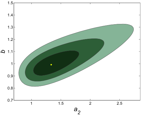
Figure 1: The 68.3%, 95.4% and 99.7% confidence contours with respect to model parameters $a_{2},~{}b$, using the Union 2 dataset. Here we assume the initial conditions are $\varphi_{0}=0.584$ and $r_{0}=5.839$. The yellow point denotes the best-fit point.

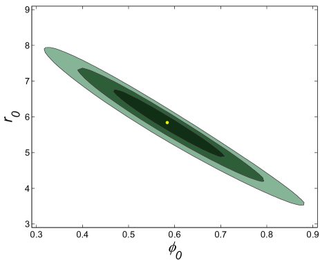
Figure 2: The 68.3%, 95.4% and 99.7% confidence contours with respect to the initial values of $\varphi_{0},~{}r_{0}$, using the Union 2 dataset. Here we assume the model parameters are $\varphi_{0}=0.584$ and $r_{0}=5.839$. The yellow point denotes the best-fit point.

V Fate of the Universe

The fate of the universe is an essential issue, which is discussed widely, for almost every cosmological model. In PGT cosmology, many works have also been conducted. In Shie:2008ms ; Chen:2009at , some numerical analyses have been done, which showed that $H$, $\Phi$ and $R$ have a periodic character at late-time of the evolution for $a_{2}>0$ and $b>0$, approximately. Some follow-up dynamics analysis and statefinder diagnostic done in Li:2009zzc ; Li:2009gj indicate that this character is corresponding to an asymptotically stable focus. And the related analytical discussion in Ao:2010mg confirmed this conclusion. However, the researches mentioned above only presented some qualitative results, where parameters $a_{2}$ and $b$ and initial values are set to certain particular positive values by hand rather than the values constrained via the observational data, and thus, quantitative analyses are still needed to be done. Therefore, in order to investigate the evolution of the real universe, it is necessary to place the constraints of parameters obtained via the SNeIa data on this model.

First we set model parameters and intial conditions to their best-fit values, and solve the evolution equations numerically. The solution of Hubble parameter and the trajectory in $H-\Phi-R$ space are plotted in Fig. 3 and Fig. 4, respectively. Then we test some other values of model parameters in the confidence interval of $3\sigma$ with fixed intial conditions which are still at the best-fit value, and plot the numerical solutions of $H(t)$ in the right column in Fig. 5. At last, we fixed the model parameters at their best-fit value, and solve the evolution equations numerically with various values of initial conditions in the confidence interval of $3\sigma$. Then we plot the results in the left column in Fig. 5. From these numerical results, it is easy to find that ($H$, $\Phi$, $R$) would tend to ($0,~{}0,~{}0$) in the far future, which indicate that our universe would expand forever asymptotically to a halt. This description of the fate of the universe is in accordance with the earlier analytical work.Ao:2010mg

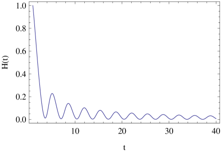
Figure 3: The late-time evolution of torsion cosmology with the best-fit values of model parameters and initial condtions for Union 2 SNeIa dataset

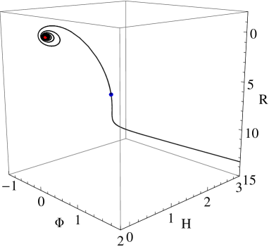
Figure 4: The evolution orbit of ($H,\Phi,R$) with the best-fit values. The blue point indicates the initial condition (1, 0.584, 5.839), whereas the red point (0, 0, 0) denotes the final state of our universe.

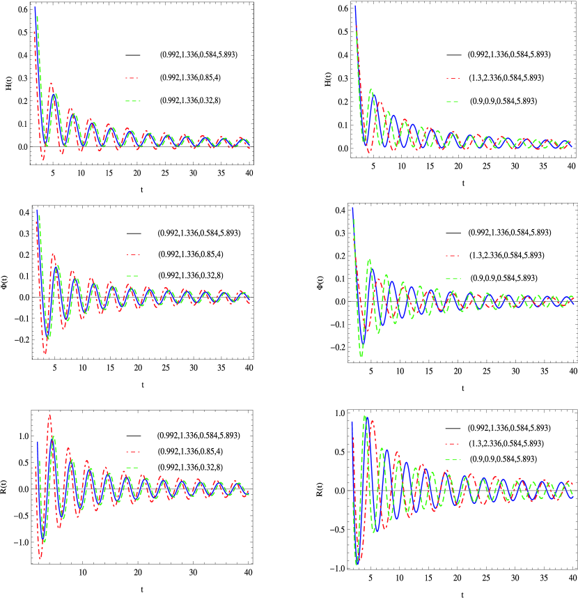
Figure 5: The late-time evolution of PGT cosmology with various values of model parameters and initial conditions lying in the confidence interval of $3\sigma$. In the left column, the model parameters are fixed at their best-fit values and the initial conditions are varied, whereas in the right column, the initial conditions are fixed at their best-fit values and the model parameters are changed.

VI Summary and Conclusion

We studied the cosmology based on PGT with even parity scalar mode dynamical connection, $0^{+}$. So the Lagrangian we use in this paper takes the form of SNY model Eq.(5). We rewrote the motion equations Eqs.(9)-Eqs.(11) as a dimensionless equation w.r.t scale factor $a$ rather than cosmological time. And we obtained the analytical solution of past time evolution of this new set of equations, as shown in Eqs.(23)-(25). Then we attempted to investigate the goodness of this model, by comparing these theoretical results with the latest observational data, Union 2 SNeIa dataset. Finally, we found the best-fit values of model parameters and initial conditions ($a_{2}=1.336,~{}b=0.992,$ $~{}\varphi_{0}=0.584$ and $r_{0}=5.839$), and that the associated minimal $\chi^{2}$ (535.284) is consistent with the $\Lambda$CDM at the 1$\sigma$ level. Furthermore, from the contours of the dynamics analysis conducted in some confidence level Fig.1 and 2, it is easy to see that, to some extent, the fine-tuning problem has been alleviated in SNY model. Next, we extended our investigation to future evolution. We plotted the whole evolution orbit of ($H,\Phi,R$), from the past to the future, with the best-fit values, in Fig. 4, which gives us a raw picture of the whole evolution. Finally, we tested some other values of parameters and initial conditions and found that $H,\Phi,R$ all tend to zero in the infinite future, which indicate our universe will expand forever asymptotically to a halt. This description of the fate of our universe is consistent with the analysis conducted above and the earlier works Li:2009zzc ; Li:2009gj ; Ao:2010mg . Thus, torsion cosmology is a ”competitive” model to explain the cosmic acceleration, which need not introduce some exotic matter composition.

In comparison to other models of accelerating universe, torsion cosmology of PGT is new, which still has a great number of issues to study. For instance, we could extend the research on SNY model to BHN model, which generalizes SNY model to a model with both $0^{\pm}$ and even the coupled term of these two modes. Also, we could investigate the effect of $0^{-}$ in the very early universe, which might has imprints in CMBR. These issues will considered in the upcoming papers.

- (1) P. J. E. Peebles and B. Ratra, The cosmological constant and dark energy, Rev. Mod. Phys. 75 (2003) 559–606, [astro-ph/0207347].
- (2) X.-Z. Li, J.-G. Hao, and D.-J. Liu, Quintessence with O(N) symmetry, Class. Quant. Grav. 19 (2002) 6049–6058, [astro-ph/0107171].
- (3) R. R. Caldwell, A Phantom Menace?, Phys. Lett. B545 (2002) 23–29, [astro-ph/9908168].
- (4) X.-Z. Li and J.-G. Hao, O(N) phantom, a way to implement w -1, Phys. Rev. D69 (2004) 107303, [hep-th/0303093].
- (5) S. Nojiri and S. D. Odintsov, Unified cosmic history in modified gravity: from F(R) theory to Lorentz non-invariant models, Phys. Rept. 505 (2011) 59–144, [arXiv:1011.0544].
- (6) Y. Du, H. Zhang, and X.-Z. Li, New mechanism to cross the phantom divide, Eur. Phys. J. 71 (2011) 1660, [arXiv:1008.4421].
- (7) H. Zhang and X.-Z. Li, MOND cosmology from holographic principle, arXiv:1106.2966.
- (8) F. W. Hehl, J. D. McCrea, E. W. Mielke, and Y. Ne’eman, Metric affine gauge theory of gravity: Field equations, Noether identities, world spinors, and breaking of dilation invariance, Phys. Rept. 258 (1995) 1–171, [gr-qc/9402012].
- (9) M. Blagojevi, Gravitation and Gauge Symmetries. IoP Publishing, Bristol, 2002.
- (10) X.-C. Ao and X.-Z. Li, de Sitter gauge theory of gravity: an alternative torsion cosmology, Journal of Cosmology and Astroparticle Physics 1110 (2011) 039, [arXiv:1111.1801].
- (11) R. Utiyama, Invariant theoretical interpretation of interaction, Phys. Rev. 101 (1956) 1597–1607.
- (12) T. W. B. Kibble, Lorentz invariance and the gravitational field, J. Math. Phys. 2 (1961) 212–221.
- (13) G. D. Kerlick, ’Bouncing’ of simple cosmological models with torsion, Annals Phys. 99 (1976) 127–141.
- (14) F. W. Hehl, Four lectures on Poincaré gauge field theory, in Proc. of the 6th Course of the School of Cosmology and Gravitation on Spin, Torsion, Rotation, and Supergravity, held at Erice, Italy, 1979 (P. G. Bergmann and V. De Sabbata, eds.), p. 5. Plenum, 1980.
- (15) K.-F. Shie, J. M. Nester, and H.-J. Yo, Torsion cosmology and the accelerating universe, Phys. Rev. D78 (2008) 023522, [arXiv:0805.3834].
- (16) H. Chen, F.-H. Ho, J. M. Nester, C.-H. Wang, and H.-J. Yo, Cosmological dynamics with propagating Lorentz connection modes of spin zero, JCAP 0910 (2009) 027, [arXiv:0908.3323].
- (17) F.-H. Ho and J. M. Nester, Poincaré gauge theory with even and odd parity dynamic connection modes: isotropic Bianchi cosmological models, arXiv:1105.5001.
- (18) F.-H. Ho and J. M. Nester, Poincaré gauge theory with coupled even and odd parity dynamic spin-0 modes: dynamic equations for isotropic Bianchi cosmologies, arXiv:1106.0711.
- (19) K. Hayashi and T. Shirafuji, Gravity from Poincaré gauge theory of the fundamental particles. 1. linear and quadratic Lagrangians, Prog. Theor. Phys. 64 (1980) 866.
- (20) K. Hayashi and T. Shirafuji, Gravity from Poincaré gauge theory of the fundamental particles. 3. weak field approximation, Prog. Theor. Phys. 64 (1980) 1435.
- (21) X.-Z. Li, C.-B. Sun, and P. Xi, Torsion cosmological dynamics, Phys. Rev. D79 (2009) 027301, [arXiv:0903.3088].
- (22) X.-Z. Li, C.-B. Sun, and P. Xi, Statefinder diagnostic in a torsion cosmology, JCAP 0904 (2009) 015, [arXiv:0903.4724].
- (23) X.-C. Ao, X.-Z. Li, and P. Xi, Analytical approach of late-time evolution in a torsion cosmology, Phys. Lett. B694 (2010) 186–190, [arXiv:1010.4117].
- (24) P. Baekler, F. W. Hehl, and J. M. Nester, Poincare gauge theory of gravity: Friedman cosmology with even and odd parity modes. Analytic part, Phys. Rev. D83 (2011) 024001, [arXiv:1009.5112].
- (25) H.-J. Yo and J. M. Nester, Hamiltonian analysis of Poincare gauge theory scalar modes, Int. J. Mod. Phys. D8 (1999) 459–479, [gr-qc/9902032].