Quasi-Biennial variations in helioseismic frequencies: Can the source of the variation be localized?

Abstract

We investigate the spherical harmonic degree ($l$) dependence of the “seismic” quasi-biennial oscillation (QBO) observed in low-degree solar p-mode frequencies, using Sun-as-a-star Birmingham Solar Oscillations Network (BiSON) data. The amplitude of the seismic QBO is modulated by the 11-yr solar cycle, with the amplitude of the signal being largest at solar maximum. The amplitude of the signal is noticeably larger for the $l=2$ and 3 modes than for the $l=0$ and 1 modes. The seismic QBO shows some frequency dependence but this dependence is not as strong as observed in the 11-yr solar cycle. These results are consistent with the seismic QBO having its origins in shallow layers of the interior (one possibility being the bottom of the shear layer extending 5 per cent below the solar surface). Under this scenario the magnetic flux responsible for the seismic QBO is brought to the surface (where its influence on the p modes is stronger) by buoyant flux from the 11-yr cycle, the strong component of which is observed at predominantly low-latitudes. As the $l=2$ and 3 modes are much more sensitive to equatorial latitudes than the $l=0$ and 1 modes the influence of the 11-yr cycle on the seismic QBO is more visible in $l=2$ and 3 mode frequencies. Our results imply that close to solar maximum the main influence of the seismic QBO occurs at low latitudes $(<45^{\circ})$, which is where the strong component of the 11-yr solar cycle resides. To isolate the latitudinal dependence of the seismic QBO from the 11-yr solar cycle we must consider epochs when the 11-yr solar cycle is weak. However, away from solar maximum, the amplitude of the seismic QBO is weak making the latitudinal dependence hard to constrain.

1 Introduction

It has been known since the mid 1980s that the frequencies of the Sun’s resonant oscillations, known as p modes, vary throughout the solar cycle with the frequencies being at their highest when the solar activity is at its maximum (e.g. Woodard & Noyes, 1985). More recently a quasi-biennial (2-year) signal has been observed in the frequencies of low-degree solar p modes (e.g. Fletcher et al., 2010, and references therein). In this paper we investigate the same quasi-biennial signal in more detail. The seismic quasi-biennial signal that we observe is highly correlated with the “quasi-biennial oscillation” (QBO) associated in other proxies of the Sun’s activity (e.g. Kane, 2005; Li et al., 2006; Ivanov, 2007; Vecchio & Carbone, 2009; Zaqarashvili et al., 2010; Badalyan & Obridko, 2011), and here we refer to the quasi-biennial signal observed in the p-mode frequencies as the “seismic” QBO. We note here that the QBO observed in other proxies of the Sun’s activity has previously been used to refer to signals with periodicities ranging from 1-3 yrs. The actual period varies depending on which epoch is considered and which proxy for solar activity is used (e.g. Kane, 2005, and references therein). There are many different methods by which a quasi-biennial modulation of the 11-yr solar cycle could be generated (e.g. Hoyng, 1990; Benevolenskaya, 1998a, b; Tobias, 2002; Wang & Sheeley, 2003; Zaqarashvili et al., 2010, and references therein), some of which involve the near-surface rotational shear layer.

The horizontal spatial structure of p modes in the Sun can be described by spherical harmonics with each mode being characterized by its spherical harmonic degree $(l)$ and azimuthal order $(m)$. The spatial structure of the oscillations means that the sectoral $|m|=l$ components of a mode are more concentrated around the equator than the zonal components, and this is particularly true as $l$ increases (see, for example, Christensen-Dalsgaard, 2002). The sectoral components are predominantly sensitive to changes in activity at lower latitudes. This is where strong-field structures, such as sunspots, dominate. On the other hand the zonal ($m=0$) components show a greater relative sensitivity to higher latitudes, where only the weak-component flux is present. Although the weak-component flux does increase slightly with the solar activity cycle it is the substantial increase in the strong-field component at low latitudes ($\leq 45^{\circ}$; de Toma, White & Harvey, 2000) that is largely responsible for the observed p-mode solar cycle variations (Howe, Komm & Hill, 1999). Therefore, the sectoral components of a p mode are more sensitive to solar cycle perturbations than the zonal components. The sizes of the shifts of different mode components scale proportionately with the corresponding spherical harmonic components of the observed line-of-sight surface magnetic field (e.g. Howe, Komm & Hill, 1999; Chaplin et al., 2003, 2004a, 2004c; Jiménez-Reyes et al., 2004; Chaplin et al., 2007b). By examining the $l$-dependence of the observed changes in frequencies throughout the solar cycle we can gain information on the latitudinal dependence of the solar magnetic field. Furthermore, the latitudinal dependence of the 11-yr solar cycle can be constrained using the frequencies of low-$l$ modes (Chaplin et al., 2007a; Chaplin, 2011).

Here we investigate whether the same constraints can be put on the latitudinal dependence of the seismic QBO, using low-$l$ modes, by examining the frequency shifts observed in modes of different $l$. Vecchio & Carbone (2009) used the green coronal emission line at 530.3 nm observed between 1939 and 2005 to examine the spatial distribution of the QBO. They found that the signal was strong in polar regions and weaker around the equator.

We make use of Sun-as-a-star (Doppler velocity) observations, which are sensitive to p modes with the largest horizontal scales (or lowest $l$). Resolved helioseismic observations allow higher-$l$ modes to be observed. However, in general these modes are more localized than are the low-$l$ modes and hence sensitive to local conditions. This has the potential to confuse the discussion of patterns on a large scale, which is what interests us here. Furthermore, the method used in the determination of frequencies for the high-$l$ modes is different from that used at low $l$ because of the influence of mode leakage, which occurs because the spatial filters are not perfect due to only half of the Sun being observed. Although analysis based on combined data sets is done, great care has to be taken to minimize systematic discrepancies (e.g. Chaplin et al., 2004a, b). Therefore, in this paper, we assess what information concerning the location of the QBO can be obtained from low-$l$ modes alone.

The structure of the remainder of this paper is as follows: Section 2 describes the data used in this paper. The $l$-dependence of the raw frequency shifts is discussed in Section 3. In Section 4 we assess whether the observed seismic QBO is strong enough to be significant when the frequencies are examined for each $l$ individually. Then, in Section 5, the $l$-dependence and frequency dependence of the seismic QBO is discussed. In Section 6 we use simple models to try and constrain the latitudinal dependence of the seismic QBO. Finally the main results are summarized in Section 7.

2 Data

The Birmingham Solar-Oscillations Network (BiSON) makes Sun-as-a-star (unresolved) Doppler velocity observations. We have used the BiSON data to investigate whether a seismic QBO is present in the frequencies of modes with $0\leq l\leq 3$, i.e. those modes that are prominent enough in Sun-as-a-star data to allow their frequencies to be determined with enough precision and accuracy to study solar cycle variations.

BiSON has now been collecting data for over 30 yrs. The time coverage of the early data, however, is poor compared to more recent data. As a consequence, here we have chosen to analyse the mode frequencies observed by BiSON from 1992 October 10 to 2011 April 7. To study the variation in the p-mode frequencies with time, the observations made by BiSON were divided into both 182.5-day-long independent subsets and 365-day-long subsets that overlapped by 91.25 d. The time series used in this paper cover a shorter epoch than the work of Fletcher et al. (2010). The start date for this analysis, i.e. 1992 October 10, was chosen because after this date the duty cycles of the 182.5-d time series were always above 60 per cent, and the average duty cycle of the subsets was 80 per cent. A high duty cycle was particularly important for determining accurately the frequencies of $l=3$ (and to a lesser extent the $l=2$) modes. This is because the heights of the individual $m$ components of these modes in a frequency-power spectrum constructed from Sun-as-a-star data are less prominent than the individual $m$ components of the $l=0$ and 1 modes. We have also classified the subsets as occurring during periods of either high- or low-surface activity. We have defined the level of surface activity to be “high” when the mean 10.7 cm flux observed in the 182.5 d independent subsets is above $100\times 10^{-22}\,\rm W\,m^{-2}\,Hz^{-1}$.

Estimates of the mode frequencies were extracted from each subset by fitting a modified Lorentzian model to the data using a standard likelihood maximization method (Fletcher et al., 2009). A reference frequency set was determined by averaging the frequencies in subsets covering the minimum activity epoch at the boundary between cycle 22 and cycle 23. It should be noted that the main results of this paper are insensitive to the exact choice of subsets used to make the reference frequency set. Frequency shifts were then defined as the differences between frequencies given in the reference set and the frequencies of the corresponding modes observed at different epochs in other subsets (Broomhall et al., 2009).

For each subset in time and each $l$ in the range $0\leq l\leq 3$, three weighted-average frequency shifts were generated, where the weights were determined by the formal errors on the fitted frequencies: first, a “total” average shift was determined by averaging the individual shifts of the modes over fourteen overtones (covering a frequency range of $1.86-3.72\,\rm mHz$); second, a “low-frequency” average shift was computed by averaging over seven overtones whose frequencies ranged from 1.86 to $2.77\,\rm mHz$; and third, a “high-frequency” average shift was calculated using seven overtones whose frequencies ranged from 2.80 to $3.72\,\rm mHz$. The lower limit of this frequency range (i.e., $1.86\,\rm mHz$) was determined by how low in frequency it was possible to accurately fit the data before the modes were no longer prominent above the background noise. The upper limit on the frequency range (i.e., $3.72\,\rm mHz$) was determined by how high in frequency the data could be fitted before errors on the obtained frequencies became too large to obtain precise values for the frequency shifts due to increasing line widths causing modes to overlap in frequency.

3 Degree dependence of frequency shifts over 11-yr solar cycle

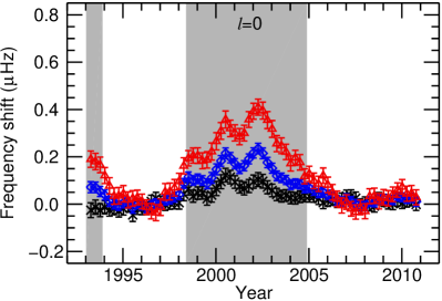
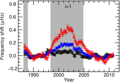
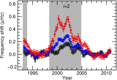
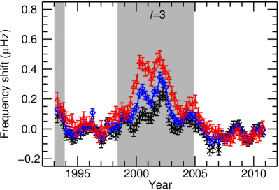
Figure 1: Individual-$l$ average frequency shifts of “Sun-as-a-star” modes observed in 365 d subsets that overlapped by 91.25 d, with frequencies between 1.86 and $3.72\,\rm mHz$ (total-frequency band, blue solid line, and diamond symbols); 1.86 and $2.77\,\rm mHz$ (low-frequency band, black dotted line, and cross symbols); and 2.80 and $3.72\,\rm mHz$ (high-frequency band, red dashed line, and triangle symbols). In each panel the shaded regions denote times of high-surface activity, while the unshaded regions denote times of low-surface activity.

Fig. 1 shows the individual-$l$ averaged frequency shifts observed in the 365 d subsets that overlapped by 91.25 d. The results from the 182.5 d subsets and the 365 d subsets are consistent and so we have chosen to plot the 365 d subsets only but we note that the 182.5 d independent subsets were used to assess the statistical significance of any signals in the frequency shifts as the overlaps in the 365 d subsets introduce artifacts in the periodicity measures we used for this purpose. The shaded regions in Fig. 1 differentiate between times of high- (shaded) and low-surface activity (unshaded).

The 11-yr solar cycle is clearly visible in the frequency shifts. For each $l$ the high-frequency range shows more sensitivity to the 11-yr cycle than the low-frequency range. This is consistent with previous observations (e.g. Broomhall et al., 2009, and references therein).

The higher-$l$ modes are more sensitive to the 11-yr solar cycle than the lower-$l$ modes. For example, the $l=2$ and 3 modes show a larger frequency shift at times of high activity than the $l=0$ and 1 modes. This is in agreement with previous observations and, as we will now explain, there are two main reasons for the observed $l$ dependence (e.g. Libbrecht & Woodard, 1990; Chaplin et al., 1998; Jiménez-Reyes et al., 2001; Salabert et al., 2009). Firstly, at fixed frequency, the mode inertia decreases with increasing degree (e.g. Howe, Komm & Hill, 1999; Chaplin et al., 2001; Rabello-Soares, Korzennik & Schou, 2008). The mode inertia (Christensen-Dalsgaard & Berthomieu, 1991) is a measure of the interior mass affected by a given mode and so, as the mode inertia decreases a smaller volume of the interior is associated with the motions generated by the mode. As such the frequencies of high-$l$ modes are more susceptible to change throughout the solar cycle than low-$l$ modes. However, the mode inertia varies very little across the modes examined here (at $3000\,\rm\mu Hz$ the inertia of an $l=0$ mode is approximately 0.3 per cent greater than the inertia of an $l=3$ mode). The second reason for the $l$-dependence of the solar cycle shifts, which is more important for low-$l$ modes than the mode inertia, is the latitudinal distribution of the solar magnetic field at the surface (e.g. Howe, Komm & Hill, 1999; Chaplin et al., 2003, 2004a, 2004c; Jiménez-Reyes et al., 2004; Chaplin et al., 2007b). Sun-as-a-star observations are most sensitive to the sectoral components of a mode, which, because of the spatial structure of the mode, show a greater sensitivity to equatorial regions as $l$ increases. Therefore, since at solar maximum the solar activity is also concentrated at low latitudes, $l=2$ and 3 modes experience a larger shift than the $l=0$ and 1 modes (when observed in Sun-as-a-star data).

Fig. 1 shows that, for each $l$, there is shorter-term, quasi-biennial structure on top of the dominant 11-yr trend and we now study this structure in more detail.

4 Assessing the significance of the seismic QBO

We begin by assessing whether the quasi-biennial structure observed in the frequency shifts represent a significant QBO. The significance of the seismic QBO was assessed by computing periodograms of the raw frequency shifts. When assessing the statistical significance of the seismic QBO we used the frequency shifts observed in the 182.5 d independent time series as artifacts can be introduced when using overlapping subsets. Overlaps in the subsets mean that the periodograms are modulated by a sinc squared function whose first zero was at $1.0\,\rm yr^{-1}$ i.e. the inverse of the time difference between independent subsets. This makes it difficult to determine whether any significant periodicities are present in the overlapping data, particularly above $0.5\,\rm yr^{-1}$.

The mean frequency shift was subtracted before each periodogram was calculated and the data were oversampled by a factor of 10. The results are shown in Fig. 2. Also plotted in Fig. 2 are the 1 per cent false alarm significance levels (Chaplin et al., 2002), which were determined using Monte Carlo simulations. 100,000 noise time series were simulated, using a normal distribution random number generator, to mimic those plotted in Fig. 1. The standard deviation of each point in the time series was taken as the $1\sigma$ error associated with the rotational splittings plotted in Fig. 1. Periodograms of the time series were calculated and the distribution of the amplitudes observed in the simulated periodograms was used to define the 1 per cent false alarm significance levels. The large peaks in each panel of Fig. 2 at $0.09\,\rm yr^{-1}$ are the signal from the 11-yr cycle.

The $l=2$ and 3 high-frequency-range periodograms show a significant peak (at a 1 per cent false alarm level) at a frequency of $\sim 0.5\,\rm yr^{-1}$. This is the same frequency as the seismic QBO observed by, for example, Fletcher et al. (2010). However, we note that Fletcher et al. also observed a significant peak at $\sim 0.5\,\rm yr^{-1}$ in low-frequency-range frequency shifts that were averaged over $0\leq l\leq 2$. However, there is no evidence for a significant signal at the same frequency in the low-frequency range observed here. We have improved our analysis techniques since Fletcher et al.. However, it is possible that this has introduced some destructive interference with noise that has reduced the amplitude of the signal. Alternatively the improved analysis could have removed constructive interference with noise that was artificially enhancing the observed signal observed by Fletcher et al.. Furthermore, Fletcher et al. examined a slightly longer time span, that included two solar maxima, which is when the seismic QBO is most prominent (this will be shown in Section 5).

A significant peak is observed at a marginally higher frequency ($\sim 0.55\,\rm yr^{-1}$) in the high-frequency-range $l=0$ periodogram. This difference would be equivalent to the resolution in a non-oversampled periodogram and so may not be significant. The $l=1$ high-frequency periodogram has a significant peak at a lower frequency ($\sim 0.35\,\rm yr^{-1}$). A significant peak at the same frequency is also present in the $l=3$ low-frequency-range periodogram. We recall that the seismic QBO has been used to refer to oscillations with periodicities ranging from 1-3 yrs. It is, therefore, possible that, despite the different periodicities, the signals observed in the different $l$ modes can be attributed to the same source.

There are two other significant peaks in the $l=3$ low-frequency-range periodogram, at 0.60 and $0.75\,\rm yr^{-1}$ respectively. The origin of these peaks is uncertain. However, we note that the peak at $0.75\,\rm yr^{-1}$ is of a similar periodicity to the 1.3-yr signal identified in other studies (e.g. Howe et al., 2000; Jiménez-Reyes et al., 2003; Wang & Sheeley, 2003; Broomhall et al., 2011).

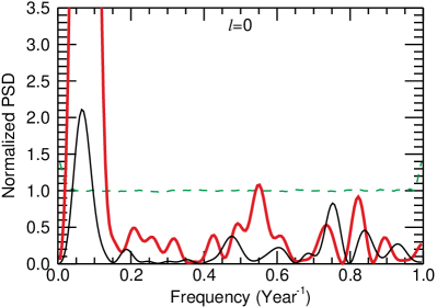
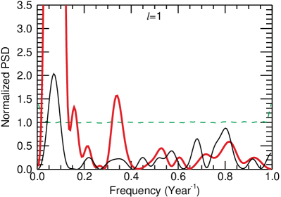
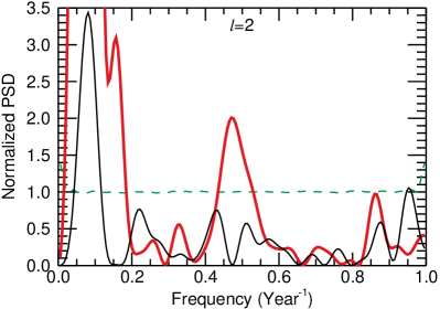
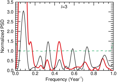
Figure 2: Periodograms of the individual-$l$ frequency shifts observed in different frequency bands using the 182.5 d independent subsets. In each panel the black thin lines are the periodograms of the low-frequency-range shifts and the red thick lines represent the high-frequency-range periodograms. The 1 per cent “false alarm” significance levels for the respective frequency ranges are also plotted (green dashed lines). The periodograms have been normalized so that for each periodogram the 1 per cent significance levels are unity. Note that the underlying resolution of a periodogram of the frequency shifts that had not been oversampled is $0.054\,\rm Year^{-1}$.

As a check of our methodology we ran the same tests on some artificial data. The data were simulated for the solar Fitting at Low Angular degree Group (solarFLAG; Chaplin et al., 2006). These data were made in the time domain and were designed to mimic Sun-as-a-star observations. The simulated oscillations were stochastically excited and damped with lifetimes analogous to those of real solar oscillations. The input mode frequencies were the same in each simulated data set and were held stationary throughout each simulated time series. However, the data simulated the stochastic nature of the mode excitation giving access to different mode and noise realizations. We have created a time series whose length was chosen to contain the same number of 182.5 d subsets as the BiSON data analyzed here. Although not shown here only one significant peak was observed in the periodograms of the frequency shifts. Furthermore, the peak was observed in the $l=3$ frequency shifts and, as we shall explain in Section 5.1, estimates of the $l=3$ mode frequencies are more noisy than the frequencies estimated for the other $l$. This indicates that we must be careful concerning the significance of the peaks observed in the $l=3$ periodograms as it is possible that the uncertainties associated with the $l=3$ frequencies underestimate the scatter in the estimated frequencies.

5 The seismic QBO

We now look at the $l$-dependence of the QBO in more detail. In order to extract the seismic QBO, we subtracted a smooth trend from the average shifts by applying a boxcar filter of width 2.5 yr. This removed the dominant 11-yr signal of the solar cycle. Note that, although the width of this boxcar is only slightly longer than the periodicity we are examining, wider filters produce similar results. The resulting residuals, which can be seen in Fig. 3 (from the overlapping 365-d subsets), show a periodicity on a timescale of about 2 yrs i.e. the seismic QBO.

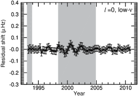
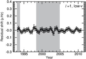
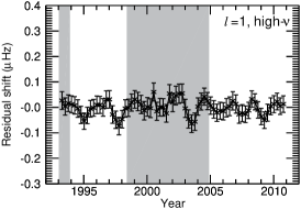
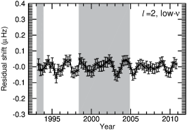
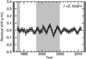
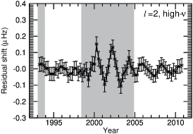
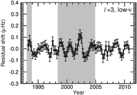
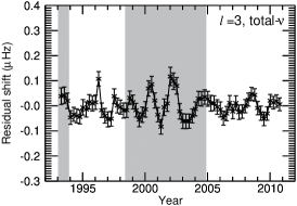
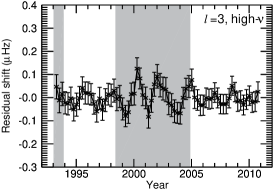
Figure 3: Individual-$l$ residuals left after the dominant 11-yr signal has been removed. The plotted results were obtained from the 365 d subsets that overlapped by 91.25 d. Right column: residuals for modes with frequencies between 1.86 and $2.77\,\rm mHz$ (low-frequency range). Middle column: residuals for modes with frequencies between 1.86 and $3.72\,\rm mHz$ (total-frequency range). Left column: residuals for modes with frequencies between 2.80 and $3.72\,\rm mHz$ (high-frequency range). First row: residuals for $l=0$ modes. Second row: residuals for $l=1$ modes. Third row: residuals for $l=2$ modes. Fourth row: residuals for $l=3$ modes. In each panel the shaded regions denote times of “high-surface activity“, while the unshaded regions denote times of “low-surface activity“.

For each $l$, the amplitude of the seismic QBO in the total- and high-frequency ranges varies with time. However, we note this is only marginally true for the $l=1$ total-frequency range. Furthermore, the amplitude of the signal in the $l=1$ total-frequency range appears to be smaller than the amplitude of the signal in the $l=1$ low- and high-frequency range because, at times, the signal in the low- and high-frequency ranges destructively interfere with each other. It could be argued that the amplitude of the seismic QBO in the total-frequency range is also smaller than in the low- and high-frequency ranges for the other $l$, although to a lesser extent. The effect is particularly evident at solar minimum.

The amplitude of the seismic QBO is larger at times of high solar surface activity than at times of low surface activity i.e. there is evidence for an 11-yr envelope on top of the seismic QBO, which is in agreement with the results of Fletcher et al. (2010). The amplitude of the envelope shows some degree dependence, being particularly visible in the $l=2$ and 3 high-frequency range residuals and less visible in the $l=0$ and 1 residuals. Notice that, for each $l$, the same envelope is barely, if at all, visible in the low-frequency-range residuals (see the left-hand panels of Fig. 3) i.e. the amplitude of the seismic QBO remains approximately constant with time. This indicates that the effect of the 11-yr cycle on the seismic QBO is, to some extent, frequency dependent.

The effect of the 11-yr envelope is further demonstrated by Table 1, which shows the maximum absolute deviations of the frequency residuals. For the high-frequency-range $l=2$ and 3 modes the maximum absolute deviation is greater at times of high activity than at times of low activity. However, the maximum absolute deviations observed in the high-frequency-range $l=0$ and 1 modes are approximately constant.

A similar dependence on the 11-yr solar cycle is also evident in the QBO in other proxies of the Sun’s activity (e.g. Benevolenskaya, 1995; Hathaway, 2010; Mursula, Zieger & Vilppola, 2003; Valdés-Galicia & Velasco, 2008; Vecchio & Carbone, 2008, 2009; Zaqarashvili et al., 2010, and references therein). The top panel of Fig. 4 shows the variation throughout the last solar cycle of the 10.7-cm radio flux ($\textrm{F}_{10.7}$) emitted from the Sun and the International Sunspot number (ISN). Many authors (e.g. Elsworth et al., 1990; Chaplin et al., 2007b; Howe, 2008, and references therein) have determined and commented upon the good correlations between shifts in the p-mode frequencies and activity proxies such as the $\textrm{F}_{10.7}$ and ISN. The bottom panel of Fig. 4 shows the residuals of the proxies once the dominant 11-yr signal has been removed (obtained by subtracting a smooth trend from the proxies). The proxies show clear evidence of the QBO, predominantly at times of high solar activity.

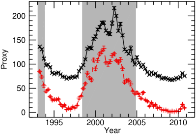
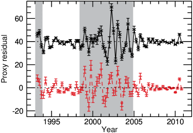
Figure 4: Top panel: Weighted mean activity proxies observed for 365 d overlapping subseries. The black solid line with the cross symbols shows the $\textrm{F}_{10.7}$, which is measured in units of $10^{-22}\,\rm W\,m^{-2}\,Hz^{-1}$. The red dashed line with the plus symbols shows the ISN. The errors on the proxies are determined using the standard error associated with a mean. Bottom panel: Residuals of the $\textrm{F}_{10.7}$ and the ISN after the dominant 11-yr signal was removed. The proxy residuals were found using 365 d overlapping subsets. The lines and symbols are the same as in the top panel. The $\textrm{F}_{10.7}$ residuals have been offset by $40\times 10^{-22}\,\rm W\,m^{-2}\,Hz^{-1}$ to ease viewing.

It is, therefore, reasonable to ask: Is there any evidence for the seismic QBO during times of low activity? Although not shown here, periodograms of the high-frequency-range frequency shifts observed during the most recent solar minimum (the unshaded region after 2005 in Fig. 1) indicate that that seismic QBO is still present, with a false alarm significance of less than 10 per cent in the $l=0$, 1, and 2 p modes. The seismic QBO is not significant at a 10 per cent threshold level in the $l=3$ modes because the errors associated with the frequency shifts are larger.

These results are not inconsistent with the conjecture that the magnetic flux responsible for the seismic QBO is situated in the near surface shear layer. Under such a scenario, when the 11-yr cycle is in a strong phase, buoyant magnetic flux sent upward from the base of the envelope could help to nudge flux produced in the near surface shear layer into shallower regions thus allowing the seismic QBO to be detected in the frequency signal. The 11-yr magnetic activity which brings the flux responsible for the seismic QBO to the surface is concentrated at low latitudes ($5^{\circ}\leq\lambda\leq 40^{\circ}$). When the 11-yr cycle is at or close to solar maximum, flux originating in the near-surface shear layer at low latitudes will be closer to the surface than the flux at higher latitudes. The influence of the flux on the p-mode frequencies is strongest when the flux is close to the surface. In Sun-as-a-star data the frequencies determined for $l=2$ and $l=3$ modes are dominated by their sectoral components ($|m|=l$; Chaplin et al., 2004a, b), which show a greater sensitivity to low latitudes than the zonal components ($m=0$).

This conjecture is consistent with the observation that the seismic QBO is stronger in the p modes and surface activity measures around solar maximum. It is also understandable that the influence of the 11-yr signal on the flux responsible for the seismic QBO is more visible in $l=2$ and 3 modes than in the $l=0$ and 1 modes.

Table 1: Maximum absolute deviations in the residuals, observed in the 365 d overlapping subsets, for the low- and high-frequency ranges (measured in $\rm\mu Hz$). The top half of the table shows the maximum absolute deviations observed during time of high solar activity i.e. before $\sim 1995$ and between 1999-2005. The bottom half of the table gives the maximum absolute deviations observed during times of low solar activity i.e. between 1995-1999 and 2005-2011 (also see for example Fig. 3).

	$l=0$	$l=1$	$l=2$	$l=3$
	During periods of high solar activity
Low	$0.04\pm 0.03$	$0.04\pm 0.02$	$0.06\pm 0.03$	$0.12\pm 0.03$
High	$0.07\pm 0.03$	$0.07\pm 0.04$	$0.14\pm 0.04$	$0.12\pm 0.05$
	During periods of low solar activity
Low	$0.03\pm 0.03$	$0.05\pm 0.02$	$0.06\pm 0.03$	$0.08\pm 0.03$
High	$0.05\pm 0.04$	$0.07\pm 0.03$	$0.04\pm 0.04$	$0.08\pm 0.05$

5.1 Constraints on the l-dependence of the seismic QBO

Monte Carlo simulations were performed to determine how constrained the observed $l$-dependence of the seismic QBO is for the entire epoch examined in this paper. For each degree 10,000 time series were simulated to contain a sine wave signal with a frequency of $0.5\,\rm yr^{-1}$, and a power spectral density comparable to that observed in the periodograms of the solar minimum frequency shifts. Noise was added to the signal, using a normally distributed random number generator, where the standard deviation of each point in the time series was taken as the $1\,\sigma$ error associated with each frequency shift plotted in Fig. 1. The simulated time series were then used to create periodograms. The simulations imply that there is more than a 90 per cent chance that the amplitude of the seismic QBO in the $l=2$ and 3 modes is greater than in the $l=0$ modes. Similarly there is more than an 80 per cent chance that the amplitude of the signal in the $l=2$ and 3 modes is greater than in the $l=1$ modes. There is a 65 per cent chance that the amplitude of the signal in the $l=1$ modes is greater than in the $l=0$ modes, while the amplitude of the signal in the $l=2$ and 3 modes is the same, to within the associated errors.

A similar analysis can be performed for the most recent solar minimum. As the $l=3$ signal is not significant during the low activity epoch we have only considered $0\leq l\leq 2$. The simulations showed that the $l$-dependence of the seismic QBO is poorly constrained by these observations and so it would be difficult to make any inferences about the latitudinal distribution of the source of the seismic QBO alone.

We also examined the $l$-dependence during the cycle 23 solar maximum i.e. 1998-2005. There is more than a 99 per cent probability that the seismic QBO in the $l=2$ p modes is greater than in both the $l=0$ and 1 p modes and there is more than a 95 per cent chance that the seismic QBO in the $l=3$ modes is greater than in the $l=0$ and 1 modes at solar maximum. The amplitude of the signal in the $l=2$ and 3 modes is the same, to within the associated errors.

Table 2: Ratios of the maximum absolute deviations of the $l=1$, 2, and 3 modes with the maximum absolute deviations of the $l=0$ modes for the high-frequency range residuals during periods of high solar activity.

$l=1$	$l=2$	$l=3$
$1.0\pm 0.7$	$2.0\pm 0.7$	$1.7\pm 0.8$

Table 2 gives the ratios between the maximum absolute deviations of the $l=1$, 2, and 3 modes and the maximum absolute deviations of the $l=0$ modes for the high-frequency range residuals during periods of high solar activity. Even at solar maximum the constraints on the $l$-dependence of the seismic QBO are not stringent and so it may be necessary to look at the frequency shifts experienced by higher-$l$ modes before any definitive conclusions can be made.

At solar maximum the seismic QBO appears to be modulated by the 11-yr solar cycle, which is known to be strongest at low latitudes, and therefore has more of an influence on the higher-$l$ modes. Therefore, the $l$-dependence of the seismic QBO at solar maximum contains information on the latitudinal dependence of both the 11-yr solar cycle and the seismic QBO such that the latitudinal dependence of the seismic QBO alone cannot be extracted. To determine the latitudinal dependence of the seismic QBO we must look at solar minimum. However, as we have shown, at this time the signal is not strong enough to constrain the $l$ dependence.

The amplitude of the QBO in the low-frequency-range $l=3$ residuals is noticeably larger than for the other $l$ (see Fig. 3 and Table 1). This could be a genuine effect: As noted in the previous section, there is a well-known dependence on $l$ in the size of the 11-yr solar cycle frequency shifts. However, we note that the estimates of the $l=3$ mode frequencies are more noisy than the frequencies estimated for the other $l$. Furthermore, estimates of the $l=3$ mode frequencies are also influenced by the nearby, much stronger, $l=1$ modes. This is partially reflected in the size of the error bars associated with the fitted frequencies (see also Figs. 1 and 3), but, as seen in Section 4 it is still possible that the uncertainties are underestimated.

5.2 The frequency dependence of the seismic QBO

Fig. 3 shows that the seismic QBO is more evident at high frequencies and it could be argued that the “signal” in the low-frequency range is just noise. This implies that the seismic QBO signal shows some frequency dependence.

We have used the 182.5 d frequencies to determine the frequency at which the seismic QBO stops being significant. To do this the weighted average frequency shifts were generated for each subset in time, in the manner described in Section 2. However, here we averaged the frequency shifts of the modes over four overtones only. The lowest frequency range for which the mean shifts were calculated was 1.86 - 2.37 mHz, i.e. the lower limit of the frequency ranges described in Section 2. The next frequency range was positioned so that it overlapped this range by 3 overtones i.e. 1.99 - 2.50 mHz. This process was repeated until the upper limit on the frequency ranges described in Section 2 was reached. In total the mean frequency shift was determined for 11 frequency ranges. We have considered the $l=2$ frequency shifts only, because over the entire epoch considered here, the seismic QBO is strongest in the $l=2$ frequencies (see Fig. 2). A periodogram of the $l=2$ frequency shifts was then determined in the manner described in Section 4. We found that the lowest frequency band at which the seismic QBO was still significant at a 1 per cent false alarm level was 2.60-3.04 mHz.

Residuals of the $l=2$ frequency shifts were then determined for the frequency bands in which the seismic QBO was significant. The maximum absolute deviations of the residuals at times of high- and low-surface activity are shown in Fig. 5. For comparison purposes the maximum absolute deviation of the raw frequency shifts was also calculated, as this reflects the amplitude of the seismic 11-yr solar cycle. Fig. 5 shows that the frequency dependence of the seismic QBO is weaker than the frequency dependence of the 11-yr solar cycle.

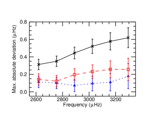
Figure 5: Maximum absolute deviations of $l=2$ residuals observed in different frequency bands. Each frequency band covers 4 overtones and the data are plotted at the frequency of the lowest overtone in each range. The red squares and the dashed line show the results for times of high-surface activity and the blue triangles and the dotted line show the results for times of low-surface activity. For comparison purposes the black crosses and the solid line show the maximum absolute deviations observed in the raw frequency shifts, which represents the amplitude of the seismic 11-yr solar cycle.

Although the 11-yr solar cycle magnetic flux is believed to be generated at the base of the convection zone the main influence of the 11-yr signal on the p-mode frequencies occurs in the upper few 100 km of the convection zone. This is above the upper turning point of the lowest frequency modes examined here and so explains the observed frequency dependence of the 11-yr cycle. Fletcher et al. (2010) postulated that the magnetic activity responsible for the seismic QBO is positioned deeper below the surface than the regions responsible for the 11-yr signal and as such the effect of the QBO on the p-modes shows a weaker frequency dependence.

Fig. 5 also shows that the frequency dependence of the seismic QBO is perhaps stronger at times of high-surface activity than at times of low-surface activity, which reflects the frequency dependence of the 11-yr envelope and again supports the idea that the 11-yr signal influences the QBO.

6 Can the degree dependence be modeled in terms of spatial distribution of magnetic field?

We now attempt to characterise the latitudinal distribution of the seismic QBO using the $l$ dependence of the signal described in Section 5, together with some simple models. Chaplin et al. (2007a) show that inferences about the spatial distribution of the 11-yr solar cycle can be made using simple models of how the latitudinal distribution of solar activity affects modes of different $l$ and $m$. Chaplin (2011) used this technique to make reasonably accurate inferences concerning the maximum latitude at which the strong field from the 11-yr solar cycle is observed. Here we determine whether similar models can be used to obtain information about the spatial distribution of the source of the seismic QBO.

We have produced a simple series of models to describe the latitudinal dependence of the magnetic activity responsible for the seismic QBO. The models are based on those used by Chaplin et al. (2007a). We took the amplitude of the magnetic activity to be uniform between some lower and upper bounds in latitude, $\lambda$, and null everywhere else. We neglect any radial dependence of the sound speed to simplify the problem. We assumed that the expected frequency shifts caused by the modeled magnetic activity were proportional to (e.g. Moreno-Insertis & Solanki, 2000)

$$\delta\nu_{lm}\propto\left(l+\frac{1}{2}\right)\frac{\left(l-m\right)!}{\left(l+m\right)!}\int_{0}^{\pi}|P_{l}^{m}(\cos\theta)|^{2}b(\theta)\sin\theta\textrm{d}\theta,$$ (1)

where $P_{l}^{m}(\cos\theta)$ are Legendre functions, while $b(\theta)$ describes the magnetic activity and, more specifically, its distribution in colatitude, $\theta=90-\lambda$. We assumed that when the frequency residuals were zero the activity responsible for the seismic QBO was zero at all latitudes, and consequently $b(\theta)=0$ for all $\theta$. When, $b(\theta)\neq 0$ for a chosen range of $\theta$, the determined $\delta\nu_{lm}$ then correspond to the amplitude of the seismic QBO.

For the chosen range of $\theta$ the magnetic flux was set to some constant value $(b(\theta)=\textrm{constant}\neq 0)$. The only parameters that were changed from model to model were the maximum and minimum latitudes at which activity was present, $\lambda_{\textrm{\scriptsize{max}}}$ and $\lambda_{\textrm{\scriptsize{min}}}$ respectively. For each combination of $\lambda_{\textrm{\scriptsize{max}}}$ and $\lambda_{\textrm{\scriptsize{min}}}$ we calculated a value for $\delta\nu_{lm}$. To summarise:

$$b(\theta)=\left\{\begin{array}[]{cl}\textrm{constant,}&\textrm{for }\lambda_{\textrm{\scriptsize{min}}}\leq|\lambda|\leq\lambda_{\textrm{\scriptsize{max}}};\\ 0,&\textrm{otherwise.}\\ \end{array}\right.$$ (2)

Note that, in the above scenario the total magnetic flux in the region of influence is proportional to the area of the Sun’s surface between $\lambda_{\textrm{\scriptsize{max}}}$ and $\lambda_{\textrm{\scriptsize{min}}}$ and therefore varied considerably over the range of computations made.

We have made no restricting assumptions over the latitudinal range over which the magnetic activity responsible for the QBO is present. So for each $\lambda_{\textrm{\scriptsize{min}}}$ in the range $0^{\circ}\leq\lambda_{\textrm{\scriptsize{min}}}<90^{\circ}$ we determined the frequency shift when $\lambda_{\textrm{\scriptsize{max}}}$ was varied between $\lambda_{\textrm{\scriptsize{min}}}<\lambda_{\textrm{\scriptsize{max}}}\leq 90^{\circ}$. The aim of this Section is then to find a combination of values for $\lambda_{\textrm{\scriptsize{max}}}$ and $\lambda_{\textrm{\scriptsize{min}}}$ that best represents the observed results.

The results in Fig. 3 show that the residuals are modulated by an 11-yr solar cycle envelope. However, according to our earlier explanation of the seismic QBO, the amplitude of the signal is enhanced at times of high activity by the 11-yr cycle and the magnitude of the enhancement is dependent on $l$. Therefore, the $l$-dependence of the amplitude of the QBO occurs because of the spatial distribution of the 11-yr solar cycle rather than the flux responsible for the seismic QBO. However, during epochs of low surface activity the signal from the seismic QBO is not strong enough to allow constraints to be put on the $l$-dependence of the signal. Therefore, we use the ratios from times of high surface activity that are shown in Table 2 to constrain the models. We also note that the Monte Carlo simulations performed in Section 5.1 imply that at solar maximum the seismic QBO in the $l=2$ and 3 modes will be larger than in the $l=1$ modes.

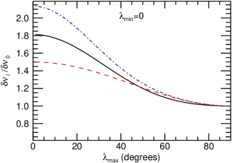
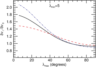
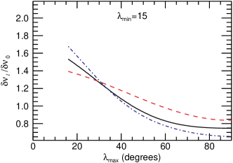
Figure 6: Ratios of the $l=1$, 2, and 3 model frequency shifts and the $l=0$ model frequency shifts given by simple models of magnetic activity. In each panel the linestyles are as follows: the red dashed line represents $l=1$; the black solid line represents $l=2$; and the blue dot-dashed line represents $l=3$.

In Sun-as-a-star data only modes where $l+m$ is even are visible, because of the near-perpendicular inclination of the solar rotation axis with respect to the Earth. When the frequency of an $l=2$ mode is obtained from Sun-as-a-star data, 90 per cent of the final frequency is determined by the $|m|=2$ components and only 10 per cent is determined by the $m=0$ component. Similarly when estimating $l=3$ frequencies 94 per cent of the final frequency is determined by the $|m|=3$ components and only 6 per cent by the $|m|=1$ components (Chaplin et al., 2004a, b). The $l=2$ and 3 model frequencies shifts were, therefore, constructed taking these percentages into account.

Ratios between the $l=1$, 2, and 3 model frequency shifts and the $l=0$ model frequency shifts were computed i.e. $(\delta\nu_{l}/\delta\nu_{0})$ and the results of a few examples of the model series are shown in Fig. 6. The top left-hand panel of Fig. 6 shows that when $\lambda_{\textrm{\scriptsize{min}}}=0^{\circ}$ the constraints on the ratios are satisfied when $\lambda_{\textrm{\scriptsize{max}}}<45^{\circ}$. As $\lambda_{\textrm{\scriptsize{min}}}$ increases the $\lambda_{\textrm{\scriptsize{max}}}$ at which the constraints are satisfied decreases. The models, therefore, imply that the QBO is strongest in equatorial regions. This is to be expected if the QBO is indeed modulated by the buoyant strong flux from the 11-yr solar cycle, which is mainly observed in equatorial regions.

7 Summary

We have shown that the seismic QBO is present in the individual-$l$ frequency shifts. The main properties of the seismic QBO are:

1. The seismic QBO in the p-mode frequencies shows an 11-yr envelope. The envelope is most visible in the $l=2$ and 3 modes but is also present in the $l=0$ and 1 p-mode frequencies. A possible explanation for the difference in the amplitude of the envelope is that close to solar maximum, the buoyant strong flux from the 11-yr cycle brings the flux responsible for the seismic QBO to the surface, where its influence on the p-mode frequencies is stronger. The buoyant strong flux from the 11-yr cycle is mainly observed at low latitudes, which the $l=2$ and 3 modes are more sensitive to than the $l=0$ and 1 modes. The $l$-dependence of the 11-yr envelope would, therefore, be influenced by the 11-yr cycle and so would not tell us about the latitudinal distribution of the seismic QBO alone.

2. To determine the latitudinal distribution of the flux responsible for the seismic QBO we must study the seismic QBO signal away from solar maximum. Although significant at a 10 per cent false alarm level, the amplitude of the seismic QBO at times of solar minimum is much smaller than at solar maximum. Therefore it was not possible to constrain the latitudinal dependence of the QBO alone.

3. We have used simple models to determine the latitudinal distribution of the flux responsible for the seismic QBO when the 11-yr cycle is at its maximum. The models imply that the $l$-dependence of the seismic QBO is best replicated when the magnetic flux is between $\pm 45^{\circ}$. This would be expected if, at solar maximum, the seismic QBO is modulated by the 11-yr cycle and the strong-field component of the 11-yr cycle is mainly observed at low-latitudes.

4. The seismic QBO is dependent on mode frequency but this frequency dependence is weaker than in the frequency shifts of the 11-yr solar cycle. The frequency dependence of the seismic QBO is stronger at solar maximum than at solar minimum. This result is consistent with the conjecture that the flux responsible for the seismic QBO is dragged to the surface by the buoyant magnetic flux of the 11-yr solar cycle at solar maximum.

In terms of the latitudinal distribution of the flux responsible for the seismic QBO, the results of this paper are by no means conclusive. To determine whether the latitudinal dependence of the seismic QBO agrees with the latitudinal distribution proposed by Vecchio & Carbone (2009), where the signal is strong in polar regions and weaker around the equator, we would need to consider times of low surface activity. Extending this study to higher-$l$, where it is possible to study a wider range of $m$ components, may help resolve this matter. However, it is also possible that, as with the low-$l$ modes, the latitudinal dependence of the seismic QBO cannot be isolated from the latitudinal dependence of the 11-yr solar cycle. Observing the Sun throughout the next solar cycle and beyond will enable better comparisons between the different $l$ to be made. The recent solar minimum has been described as unusual because of its depth and longevity. It will be interesting, therefore, to compare the seismic QBO observed in the upcoming solar cycle with that observed in the last.

References

- Badalyan & Obridko (2011) Badalyan O. G., Obridko V. N., 2011, NewA., 16, 357
- Benevolenskaya (1995) Benevolenskaya E. E., 1995, Sol. Phys., 161, 1
- Benevolenskaya (1998a) —, 1998a, ApJL, 509, L49
- Benevolenskaya (1998b) —, 1998b, Sol. Phys., 181, 479
- Broomhall et al. (2009) Broomhall A., Chaplin W. J., Elsworth Y., Fletcher S. T., New R., 2009, ApJL, 700, L162
- Broomhall et al. (2011) Broomhall A. et al., 2011, Journal of Physics Conference Series, 271, 012025
- Chaplin (2011) Chaplin W. J., 2011, Lecture Notes of the 22nd Canary Island Winter School
- Chaplin et al. (2006) Chaplin W. J. et al., 2006, MNRAS, 369, 985
- Chaplin et al. (2004a) Chaplin W. J., Appourchaux T., Elsworth Y., Isaak G. R., Miller B. A., New R., 2004a, A&A, 424, 713
- Chaplin et al. (2004b) Chaplin W. J., Appourchaux T., Elsworth Y., Isaak G. R., Miller B. A., New R., Toutain T., 2004b, A&A, 416, 341
- Chaplin et al. (2001) Chaplin W. J., Appourchaux T., Elsworth Y., Isaak G. R., New R., 2001, MNRAS, 324, 910
- Chaplin et al. (2007a) Chaplin W. J., Elsworth Y., Houdek G., New R., 2007a, MNRAS, 377, 17
- Chaplin et al. (1998) Chaplin W. J., Elsworth Y., Isaak G. R., Lines R., McLeod C. P., Miller B. A., New R., 1998, MNRAS, 300, 1077
- Chaplin et al. (2002) Chaplin W. J., Elsworth Y., Isaak G. R., Marchenkov K. I., Miller B. A., New R., Pinter B., Appourchaux T., 2002, MNRAS, 336, 979
- Chaplin et al. (2004c) Chaplin W. J., Elsworth Y., Isaak G. R., Miller B. A., New R., 2004c, MNRAS, 352, 1102
- Chaplin et al. (2003) Chaplin W. J., Elsworth Y., Isaak G. R., Miller B. A., New R., Thiery S., Boumier P., Gabriel A. H., 2003, MNRAS, 343, 343
- Chaplin et al. (2007b) Chaplin W. J., Elsworth Y., Miller B. A., Verner G. A., New R., 2007b, ApJ, 659, 1749
- Christensen-Dalsgaard (2002) Christensen-Dalsgaard J., 2002, Reviews of Modern Physics, 74, 1073
- Christensen-Dalsgaard & Berthomieu (1991) Christensen-Dalsgaard J., Berthomieu G., 1991, Theory of solar oscillations., Solar Interior and Atmosphere, pp. 401–478
- de Toma, White & Harvey (2000) de Toma G., White O. R., Harvey K. L., 2000, ApJ, 529, 1101
- Elsworth et al. (1990) Elsworth Y., Howe R., Isaak G. R., McLeod C. P., New R., 1990, Nature, 345, 322
- Fletcher et al. (2010) Fletcher S. T., Broomhall A., Salabert D., Basu S., Chaplin W. J., Elsworth Y., García R. A., New R., 2010, ApJL, 718, L19
- Fletcher et al. (2009) Fletcher S. T., Chaplin W. J., Elsworth Y., New R., 2009, ApJ, 694, 144
- Hathaway (2010) Hathaway D. H., 2010, Living Reviews in Solar Physics, 7, 1
- Howe (2008) Howe R., 2008, Advances in Space Research, 41, 846
- Howe et al. (2000) Howe R., Christensen-Dalsgaard J., Hill F., Komm R. W., Larsen R. M., Schou J., Thompson M. J., Toomre J., 2000, Science, 287, 2456
- Howe, Komm & Hill (1999) Howe R., Komm R., Hill F., 1999, ApJ, 524, 1084
- Hoyng (1990) Hoyng P., 1990, in IAU Symposium, Vol. 138, Solar Photosphere: Structure, Convection, and Magnetic Fields, J. O. Stenflo, ed., pp. 359–+
- Ivanov (2007) Ivanov E. V., 2007, Advances in Space Research, 40, 959
- Jiménez-Reyes et al. (2001) Jiménez-Reyes S. J., Corbard T., Pallé P. L., Roca Cortés T., Tomczyk S., 2001, A&A, 379, 622
- Jiménez-Reyes et al. (2004) Jiménez-Reyes S. J., García R. A., Chaplin W. J., Korzennik S. G., 2004, ApJL, 610, L65
- Jiménez-Reyes et al. (2003) Jiménez-Reyes S. J., García R. A., Jiménez A., Chaplin W. J., 2003, ApJ, 595, 446
- Kane (2005) Kane R. P., 2005, Sol. Phys., 227, 155
- Li et al. (2006) Li K. J., Li Q. X., Su T. W., Gao P. X., 2006, Sol. Phys., 239, 493
- Libbrecht & Woodard (1990) Libbrecht K. G., Woodard M. F., 1990, Nature, 345, 779
- Moreno-Insertis & Solanki (2000) Moreno-Insertis F., Solanki S. K., 2000, MNRAS, 313, 411
- Mursula, Zieger & Vilppola (2003) Mursula K., Zieger B., Vilppola J. H., 2003, Sol. Phys., 212, 201
- Rabello-Soares, Korzennik & Schou (2008) Rabello-Soares M. C., Korzennik S. G., Schou J., 2008, Advances in Space Research, 41, 861
- Salabert et al. (2009) Salabert D., García R. A., Pallé P. L., Jiménez-Reyes S. J., 2009, A&A, 504, L1
- Tobias (2002) Tobias S. M., 2002, Astronomische Nachrichten, 323, 417
- Valdés-Galicia & Velasco (2008) Valdés-Galicia J. F., Velasco V. M., 2008, Advances in Space Research, 41, 297
- Vecchio & Carbone (2008) Vecchio A., Carbone V., 2008, ApJ, 683, 536
- Vecchio & Carbone (2009) —, 2009, A&A, 502, 981
- Wang & Sheeley (2003) Wang Y., Sheeley, Jr. N. R., 2003, ApJ, 590, 1111
- Woodard & Noyes (1985) Woodard M. F., Noyes R. W., 1985, Nat., 318, 449
- Zaqarashvili et al. (2010) Zaqarashvili T. V., Carbonell M., Oliver R., Ballester J. L., 2010, ApJL, 724, L95